Article

A Linear Interpolation Method for Five-Axis Machining Paths on Fan Blisk Surfaces with Constant Theoretical Machining Error

by
Zhiwei Wang
1,*,
Yingjian Tian
1,
Shuanglong Mao
2,
Zhanwang Shi
1 and
Hengdi Wang
1
1
School of Mechatronics Engineering, Henan University of Science and Technology, Luoyang 471003, China
2
Aecc South Industry Company Limited, Zhuzhou 412000, China
*
Author to whom correspondence should be addressed.
Machines 2025, 13(9), 768; https://doi.org/10.3390/machines13090768
Submission received: 27 July 2025 / Revised: 19 August 2025 / Accepted: 25 August 2025 / Published: 28 August 2025
(This article belongs to the Section Advanced Manufacturing)

Abstract

Blisks are complex thin-walled parts with specific structures that have narrow channels and a large degree of bowed-twisted blades. Five-axis machining technology critically influences blisk surface quality and production efficiency, as the toolpath determines machining accuracy for complex curved blades. A method of optimal cutter location calculation for linear interpolation path based on the constraint of equal theoretical machining error is proposed. Based on the kinematics model of the machine tool, the mapping relationship between the trajectory deviation of the five-axis of machine tool and the tool pose deviation in the workpiece coordinate system is established, and then the maximum overcut/undercut value under the coupling action of the tool tip deviation and the tool orientation deviation is estimated. Based on this, a method to estimate the upper limit of theoretical machining error caused during the movement of the tool along the linear path is proposed. And the algorithm for searching discrete cutter locations on the trajectory of cutting contacts is given to maximize the length of linear path based on the constraint of equal machining error. Experimental results demonstrate that the proposed method effectively reduces redundant cutter locations on linear paths and enhances blisk surface quality by replacing conventional constant chord error control with a more preblisk machining error constraint.

1. Introduction

Blisks are complex thin-walled parts with specific structures that have narrow channels and a large degree of bowed-twisted blades. The blisk integrates the blades and disk into a single monolithic structure, thereby reducing part count and weight, minimizing aerodynamic losses, and preventing potential crack initiation and propagation at joints. Future engines featuring high thrust-to-weight ratios and large bypass ratios will necessitate even more complex blisk geometries, imposing stricter requirements on manufacturing technologies [1,2]. Five-axis Computer Numerical Control (CNC) machining technology has gained widespread application in the manufacturing of large fan blisks due to its advantages of rapid response, high reliability, excellent machining flexibility, and short production lead time [3,4,5]. The axis machining technology is directly relevant to blisk surface quality and production, and it remains one of the bottlenecks restricting the development of high-performance aero-engines.
Prior studies concerning the milling of blisks indicate that machining free-form blade surfaces entails considerable difficulties. These challenges stem from pronounced surface distortions, diversity in milling techniques (such as end milling and flank milling), and complexities in toolpath design, tool geometry, and machining parameter optimization. These factors collectively cause a significant deviation between the ideal tool envelope and the actual surface to be machined. Yan et al. [6] and Zhou et al. [7] provided comprehensive overviews on semi-finishing and finishing operations for blade curved surfaces, with emphasis on process design, dynamic milling behavior, error estimation, vibration evaluation, and surface integrity. Toolpath generation is influenced by the milling strategy adopted and must accommodate variables like tool geometry, potential machining interference, collision avoidance, and dynamic properties of the machine tool [8,9,10,11].
Based on the distinct interaction modes between the cutting tool and the workpiece, the current machining of blisks primarily utilizes two strategies: end milling and flank milling. Owing to differences in their fundamental machining mechanisms and operational processes, the two methods lead to variations in machining precision, efficiency, and surface quality [11,12]. Moreover, differences in tool geometry and the cutter–workpiece engagement (CWE) require distinct emphases in toolpath planning for each technique. In end milling, the primary objective is to minimize the total toolpath length to improve machining efficiency. In contrast, flank milling focuses on generating toolpaths that produce an unbiased enveloping surface between the tool and the designed blade shape [13,14,15]. This involves meticulous planning of the tool geometry, tool orientation, and trajectory paths to ensure that the envelope formed at the CWE accurately matches the predefined free-form surface.
The leading and trailing edges of the blades are thin and exhibit sharp curvature changes, which can easily induce axis wobble, resulting in variable cutting speeds and eventual chatter [3,7]. Therefore, developing an effective toolpath interpolation strategy is essential to achieve high quality and efficiency for the five-axis machining of fan blisks. Current five-axis toolpath interpolation methods primarily include linear interpolation, circular interpolation, and spline curve interpolation. Although parametrically continuous interpolation techniques, such as Non-Uniform Rational B-Splines (NURBS), enable smooth motion of both tool position and orientation, significantly reducing program volume and effectively suppressing velocity fluctuations, they rely on high-end CNC systems (e.g., Siemens 840D sl) [15,16]. In contrast, linear interpolation (G01 code) remains the mainstream technical solution for complex surface machining, owing to its seamless compatibility with existing CAD/CAM workflows, broad support from general-purpose CNC systems, and relative simplicity in handling tool axis singular regions [17,18,19].
Currently, for NURBS-based theoretical toolpath curves in five-axis machining, the planning of cutter location points for linear interpolation is primarily carried out using two approaches: the constant chord height tolerance [20,21,22], the equal parameter [23,24], and constant theoretical machining error [25,26,27]. Both of them primarily ensure the deviation between the interpolated toolpath and the ideal path within the workpiece coordinate system. The main characteristics of the three methods are as follows:
  • Method based on constant chord height tolerance: It employs a curvature-adaptive step size strategy to constrain theoretical machining error approximated by controlling the deviation between the linear toolpath and the interpolated curve path. It is suitable for machining free-form surfaces with gentle variations in both the tool axis direction and the curvature of the machined surface.
  • Method based on equal parameter: The maximum deviation distance between the linear toolpath and the interpolated curve path is indirectly controlled by setting a threshold with fixed parameter intervals. It is suitable for rough machining simple surfaces with gentle curvature variations.
  • Method based on theoretical machining error: The constant machining error method primarily obtains cutter location points by screening for suitable cutter axis vector directions to achieve the deviation between the tool swept envelope surface and the ideal machined surface. It is widely used for flank milling of developable ruled surfaces.
Those approaches focus solely on positional approximation accuracy and fail to address the unique nonlinear errors inherent in five-axis machining [28,29]. Specifically, during angular linear interpolation of rotary axes, the nonlinear mapping between rotary motion and Cartesian space causes the actual tool axis vector to deviate from the ideal geodesic plane. This deviation results in significant uncontrollable orientation errors [3,30,31].
At the kinematic response level, traditional methods inadequately consider the impact of machine tool dynamic characteristics on machining errors [32,33,34,35,36]. Dense micro-line segments trigger frequent acceleration/deceleration, causing feed rate fluctuations. Rotational axis angular velocity experiences abrupt changes near singular points, easily inducing machine tool chatter [32,33]. Then the lag differences in servo response between linear and rotary axes cause spatial trajectory distortion. Studies confirm that rotational axis velocity fluctuates under linear interpolation mode. While vector plane interpolation can eliminate nonlinear errors, it exacerbates the nonlinear variation of angular acceleration, leading to a significant increase in chatter mark amplitude on the machined surface [34,37]. Notably, traditional methods rely on empirical coefficients to adjust error control parameters, where chord error thresholds and nonlinear error tolerances are typically set based on process experience.
Based on the analysis mentioned above, it is apparent that a considerable number of researchers have extensively investigated strategies for toolpath planning in free-form surface machining, as well as methods to mitigate machining-induced deformations during the milling of thin-walled blade of fan blisks, with the aim of improving both accuracy and efficiency. However, there is a lack of methods for optimizing the cutter locations of linear interpolation paths with constant theoretical machining error. In this paper, a linear interpolation method for five-axis machining paths on fan blisk surfaces with constant theoretical machining error is proposed. In Section 2, the kinematics model of the machine tool is established, along with the mapping relationship between the trajectory deviations of the machine tool axes and the tool pose deviation. In Section 3, the maximum overcut/undercut values under the coupled effect of tool tip deviation and tool orientation deviation are estimated. Then the algorithm for searching discrete cutter locations is given. The proposed method is verified and evaluated in Section 4. Finally, the work is concluded in Section 5.

2. Deviation in Linear Interpolation Toolpath for Five-Axis Machining of Blisk

2.1. Causes of Toolpath Deviation

The fan blisk consists of an inner hub and blades, as shown in Figure 1. The surface of blade of the fan blisk is often designed with a NURBS-based free-form surface and can be divided into four parts: the trailing edge, leading edge, blade convex, and blade concave. The curvature of the section curve between the trailing edge and leading edge intervals is large and changes abruptly, while the curvature of the remaining intervals is small and changes gradually. During the process of five-axis machining of the blisk, a continuous helical toolpath is typically employed, which extends from the top to the inner hub and is both long and periodic. In the prebliskion machining of blisk surfaces, a parametric curve is typically employed as the tool contact path trajectory to achieve a cutting texture that aligns with the direction of airflow. Furthermore, to prevent tool marks at the junction point resulting from tool changes, a single tool is generally utilized for continuous machining along the stacking axis, extending from the blade tip to the inner hub. However, during the five-axis machining of the integral blade disk, the frequent acceleration and deceleration of each motion axis can adversely affect surface quality. Additionally, significant machining errors are more likely to occur in the leading and trailing edge regions of the blade due to the abrupt changes in the tool trajectory, as illustrated in Figure 1b.
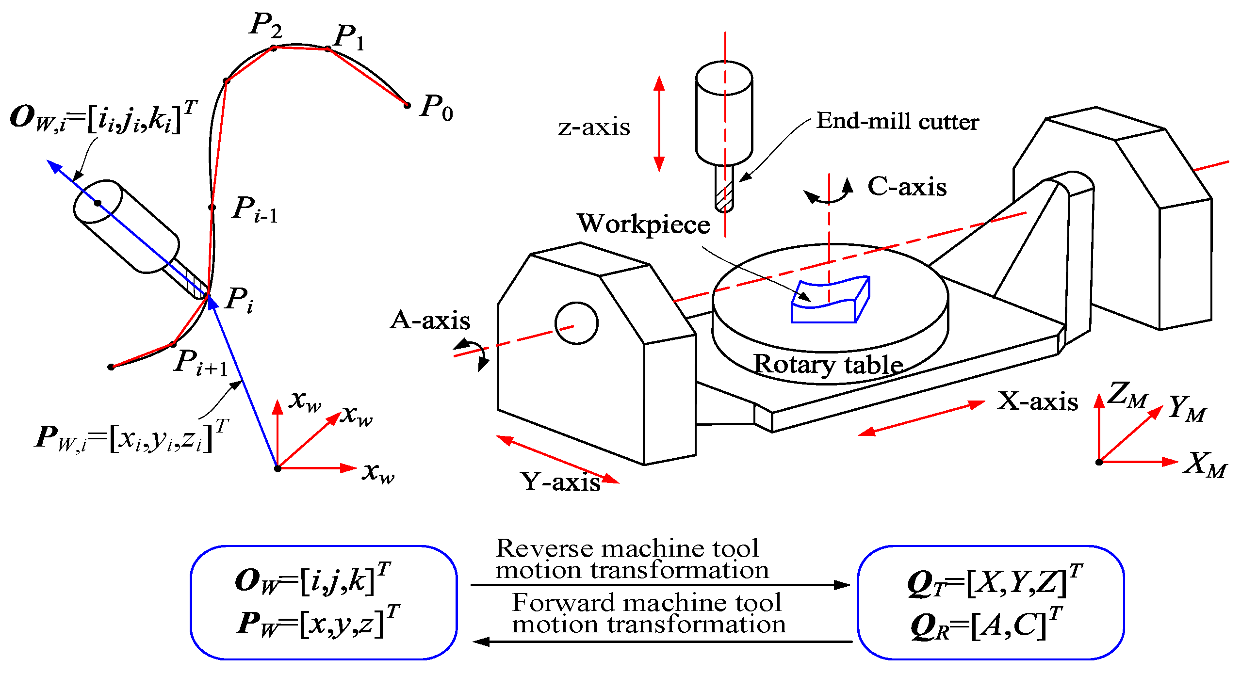
Five-axis machining of curved surfaces is achieved by controlling the displacement of three linear motion axes and two rotary axes of the machine tool through the CNC system, which in turn drives the tool to move continuously along the planned vector path of the tool tip point and the tool axis, as illustrated in Figure 2. In the workpiece coordinate system, the toolpath consists of the tool tip position and the matching tool axis vector. In this case, the position of the tool tip point on the toolpath is represented by PW = [x,y,z]T, while the tool axis vector at point Pi is denoted by the unit vector OW = [i,j,k]T. In the machine tool coordinate system, the displacement of the machine tool motion axes is typically expressed using the five-parameter QM = [QMT, QMR]. Here, QMT = [X,Y,Z]T refers to the displacement of the three linear motion axes of the machine tool, whereas QMR = [A,C]T indicates the displacement of the two rotary motion axes. When the CNC machine tool executes the G01 instruction for linear motion, both the linear motion axis and the rotary motion axis are driven by servomotors so that their displacements move along the linear path line segments.
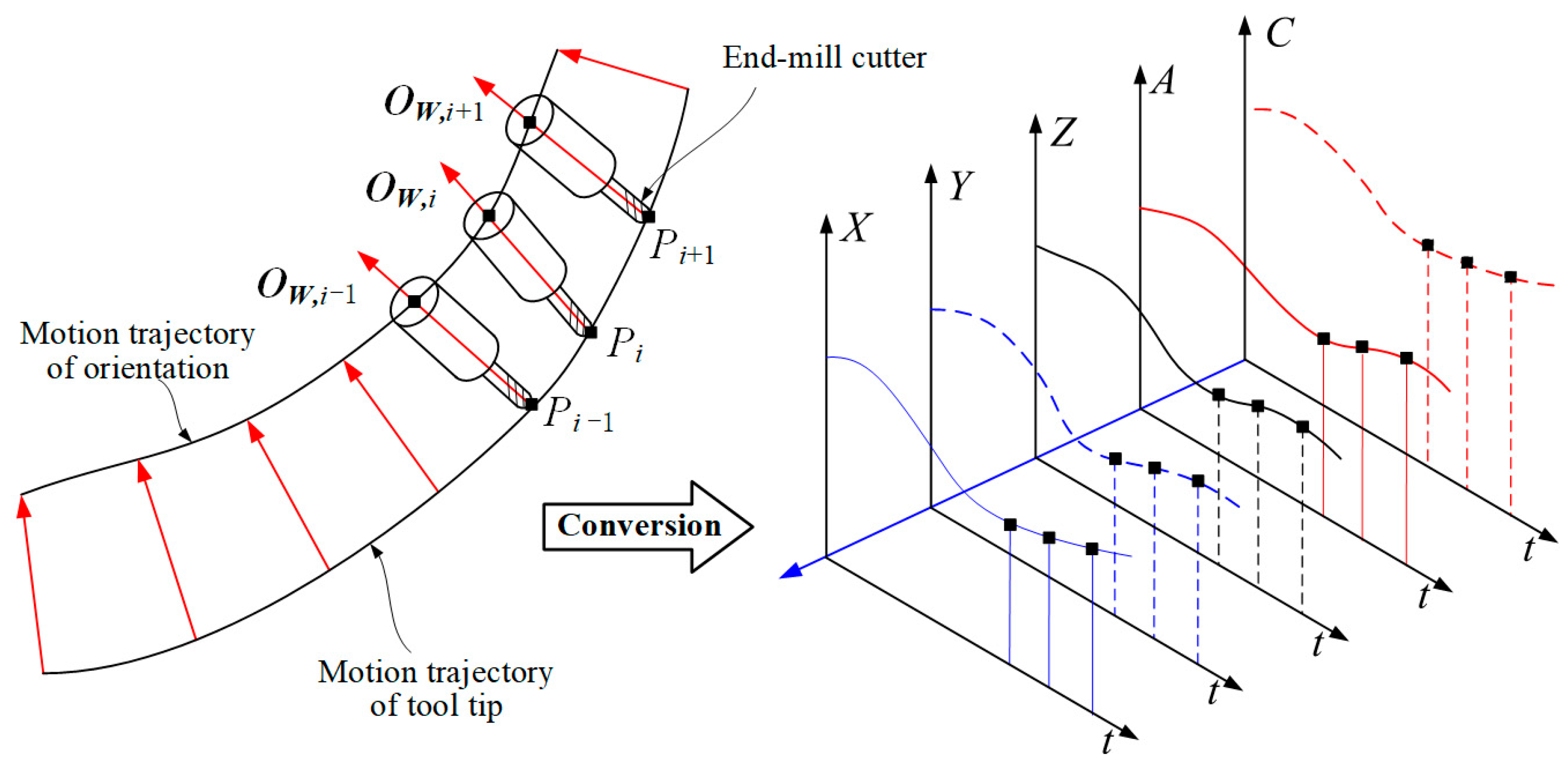
When executing the G01 command for linear paths, CNC machine tools drive both linear and rotary motion axes through servomotors, causing each axis to move along straight-line segments as shown in Figure 3. At the start- and endpoints of the linear path, the displacements of the machine’s two rotary axes synthesize the tool axis orientation, ensuring the relative positional relationship between the tool and workpiece conforms to the tool axis vector defined in the workpiece coordinate system. Simultaneously, the displacements of the machine’s three linear motion axes and two rotary motion axes jointly synthesize the tool tip point, maintaining its relative position to the workpiece surface consistent with the state specified in the workpiece coordinate system. Between the start- and endpoints of the linear path, all machine motion axes move proportionally and synchronously along the straight-line segment. In the calculation method for cutter location points during linear interpolation of curves based on the workpiece coordinate system, the theoretical machining errors caused by interpolation must be further transformed to the machine coordinate system for evaluation. The theoretical trajectory of the tool for smooth five-axis machining of complex surfaces is interpolated by curved straight lines to produce a tool position file, which in turn is subsequently executed as G01 code in the CNC. In this case, the smooth theoretical tool trajectory is interpolated by a curved straight line to generate the initial and final linear paths. This process results in interpolation errors due to the replacement of curves with straight lines.
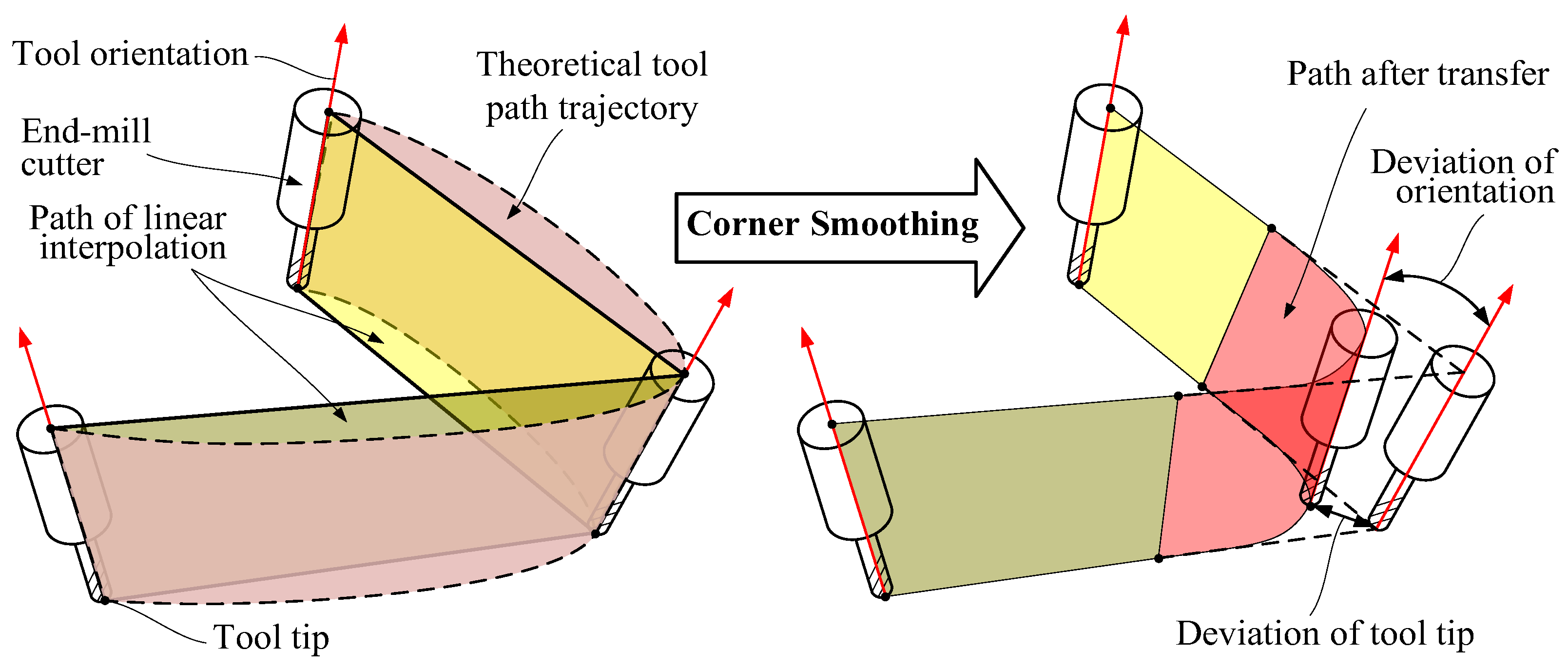
In order to ensure the continuous speed of each axis of the machine tool and to improve the machining efficiency, the CNC system will realize the higher-order continuity of the transfer curve and the connection of the linear line segments by inserting smooth micro-curves at the corners of the adjacent linear paths, which introduces the corner transfer bias of replacing the straight with the curved one. Both errors arising from linear interpolation and those generated by corner transfers can cause the tool to deviate from its intended ideal position. The discrepancy between the actual position of the tool and its theoretical position is referred to as tool position deviation. This deviation encompasses both the tip point deviation and the tool orientation, as illustrated in Figure 4. This deviation would lead to theoretical machining error during processing. This theoretical machining error results from approximating a smooth curve path with a series of connected linear segments. The linear toolpath in the workpiece coordinate system needs to be converted into a drive command in the machine tool coordinate system for processing. Consequently, the deviation between the actual and theoretical trajectories of the linear and rotary axes of the machine tool more accurately reflects the discrepancy between the actual and theoretical toolpaths following linear interpolation and corner transfer. To rationally plan the five-axis machining toolpaths for the inlet and exhaust edges of the curved surface of the entire blade disk, this paper performs straight-line interpolation along the trajectory curve within the machine tool’s coordinate system. This approach aims to reduce redundancy in tool position points while ensuring machining accuracy.

2.2. Linear Interpolation Deviation of Motion Trajectory of 5-Axis Machining Machine Tool

Deviations between the trajectories of the machine tool axes of motion and the theoretical curve path during the execution of linear and transfer curve paths will cause the tool to deviate from the theoretical position. In this case, the deviation of the machine tool motion trajectory is measured as the directed distance between the actual position and the theoretical curve path, which consists of the linear motion axis trajectory deviation and the rotary axis trajectory deviation. In addition, the linear path local transfer smoothness is achieved by inserting a smooth and symmetric micro-B spline curve to replace certain segments of the original line at the angles formed by two ordered adjacent line segments. This insertion is interpolated in real time by the numerical control system during the execution of the G01 instruction, resulting in a minimal deviation. The specific construction process and the calculation of this deviation can be found in the literature [9] and will not be reiterated in this paper. It is noted that an increase in the curvature of the corner transfer curve results in a decreased allowable feed rate, which subsequently leads to diminished machining quality and efficiency. Therefore, it is essential to minimize the transfer angle between adjacent linear paths to reduce the curvature of the corner transfer curve.
In the machine tool coordinate system, the value of the trajectory deviation of the machine tool linear and rotary axes of motion at any position on the linear path can be described by the bow-height difference generated by the microlinear segment approximation curve, as illustrated in Figure 5. The theoretical motion trajectory curve path of the linear motion axis of the machine tool is denoted by CT(v), while the i-th discrete point on the curve is represented by CT(vi). Similarly, the theoretical motion trajectory curve path of the rotary motion axis of the machine tool is denoted by CR(v), while the i-th discrete point on the curve CR(v) is represented by CR(vi). The curve CT(v) and CR(v) parameters are synchronized, while vi is the curve parameter common to the discrete points CT(vi) and CR(vi). Denote the curve parameter at the maximum deviation on the curve CT(v) as vT,i. The directed distance between the point CT(vT,i) and the line segment CT(vi−1)CT(vi) is the maximum deviation; denote it by εT,i. Similarly, between points CR(vi−1) and CR(vi), the curve parameter at the maximum deviation along curve CR(v) of the machine tool’s rotary axis motion trajectory is denoted as vR,i. The distance from point CR(vR,i) to line segment CR(vi−1)CR(vi) represents the maximum deviation value, denoted as εR,i. After performing linear interpolation on the five-axis machining curves, linear paths are generated by substituting the curve segments C T ( v i     1 ) C T ( v i ) and C R ( v i     1 ) C R ( v i ) with straight-line segments CT(vi−1)CT(vi) and CR(vi−1)CR(vi), respectively. The deviation values εT,i and εR,i represent the deviation of the linear interpolation machine movement. Since the corner transfer between linear path segments is regulated by a numerical control system, and given that the deviation value is minimal, this article will not address it further.
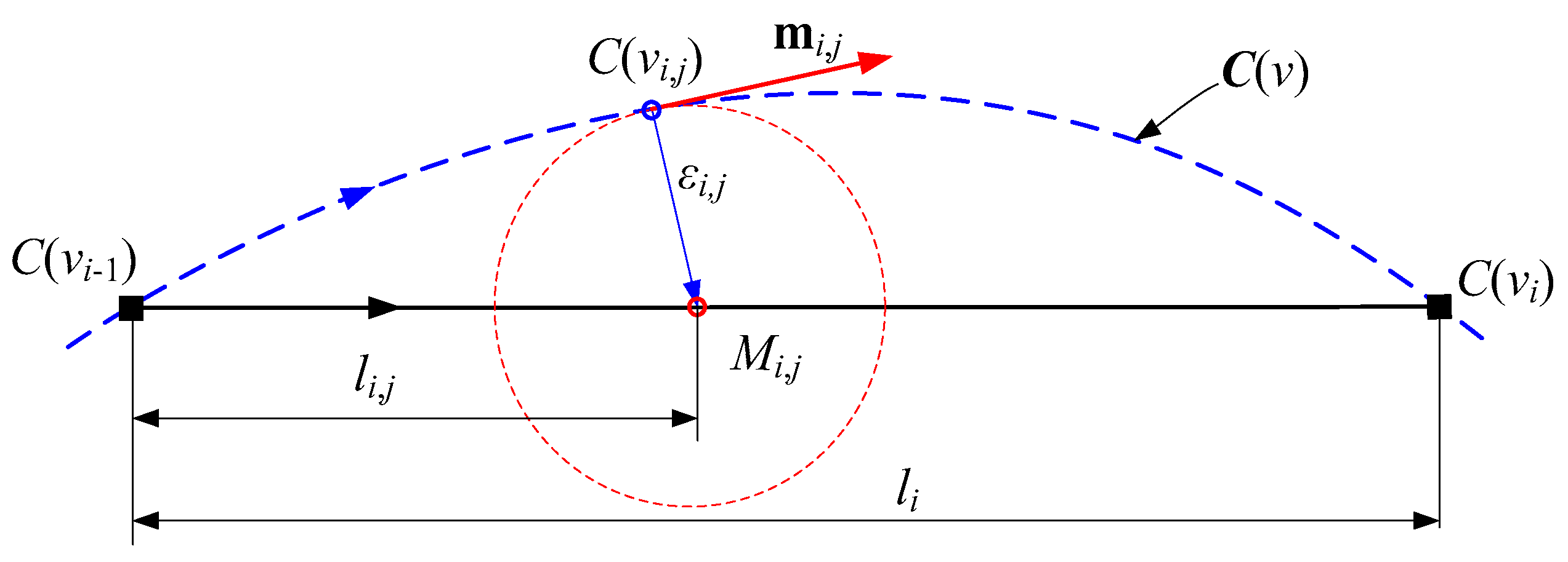
The motion deviation of both linear and rotary motion axes of the machine tool can be determined by calculating the maximum directed distance between the actual trajectory and the theoretical motion trajectory, as illustrated in Figure 6. The theoretical motion trajectory curve of the machine tool is uniformly represented by C(v), with the i-th discrete point on this curve denoted as C(vi), where vi is the curve parameter at the discrete point. The straight-line segment C(vi−1)C(vi), which connects neighboring discrete points, serves as the linear interpolation path along the curve segment C ( v i     1 ) C ( v i ) . The jth arbitrary discrete point on the linear path C(vi−1)C(vi) is denoted as Mi,j, while the point on the curve segment C ( v i     1 ) C ( v i ) that is closest to point Mi,j is referred to as C(vi,j). The directed distance between points C(vi,j) and Mi,j represents the deviation of the motion trajectory of the machine tool motion axis when it is tracked to point Mi,j along the linear path segment C(vi−1)C(vi), where the value of the machine tool motion trajectory deviation is denoted by εi,j, and its direction is represented by C ( v i , j ) M i , j .
Point Mi,j on the straight-line segment C(vi−1)C(vi) corresponds to point C(vi,j) on the curve segment C ( v i     1 ) C ( v i ) . Point Mi,j can be considered the intersection of the normal plane at point C(vi,j) on curve C(v) and the straight-line segment C(vi−1)C(vi). The tangent vector along the direction of motion at point C(vi,j) on curve C(v) is denoted as mi,j. This vector is mutually perpendicular to the vector C ( v i , j ) M i , j , satisfying Equation (1).
m i , j C ( v i , j ) M i , j = 0
In Equation (1), vector mi,j and vector C ( v i , j ) M i , j can be expressed by Equation (2).
m i , j = d C ( v ) d v v = v i , j , C ( v i , j ) M i , j = C ( v i     1 ) C ( v i , j ) + l i , j C ( v i     1 ) C ( v i ) C ( v i 1 ) C ( v i )
In Equation (2), li,j is the distance between point C(vi−1) and point Mi,j.
The deviation direction of the interpolated curve path of the straight-line segment is the same as that of the vector C ( v i , j ) M i , j , while the deviation value εi,j can be calculated from Equation (3).
ε i , j = C ( v i , j ) M i , j

2.3. Deviation Conversion of Trajectory from Machine Tool to Tool

Since machining errors need to be described within the workpiece coordinate system, it is essential to establish a correspondence between the trajectory deviations of the machine tool motion axes and the positional deviations of the tool. The trajectories of the machine tool axes of motion undergo a nonlinear transformation relative to the tip point and the tool axis. Furthermore, the transformation from the machine tool coordinate system to the workpiece’s coordinate system fails to satisfy curvilinear geometric invariance. When the position of the machine tool’s motion axis is specified, the tool pose in the workpiece coordinate system can be calculated based on the forward machine tool motion model. By deriving both sides of the equals sign of the forward motion model of the machine tool with respect to time, we obtain the Jacobian matrix of the machine tool motion model. This matrix describes the linear relationship between the changes in the displacements of the machine tool motion axes and the amount of change in the tool orientation within the workpiece coordinate system, as illustrated in Equation (4).
d P W d O W = J d Q M = J T T J T R J R T J R R d Q M T d Q M R
In Equation (4), the Jacobian matrix J is composed of four sub-matrices. And for the symbols of JTT, JTR, JRT, and JRR, the first subscripts T and R of the sub-matrix denote the affected tool tip point and tool axis vector, respectively, while the second subscripts T and R of the sub-matrix represent the influence of the linear motion axis and rotational motion axis of the machine tool on the tool attitude, respectively.
According to the rules of chunked matrix operations, Equation (4) is equivalent to Equation (5).
d P W = J T T d Q M T + J T R d Q M R d O W = J R T d Q M T + J R R d Q M R
Since the tool axis vector is unaffected by the linear axes of motion of the machine, the matrix JRT = 0. And the matrices JTT, JRR, and JTR are presented in Equation (6).
J T T = cos C cos A sin C sin A sin C sin C cos A cos C sin A cos C 0 sin A cos A , J R R = cos A sin C sin A cos C cos A cos C sin A sin C sin A 0 J T R = ( Z     Y ) sin A sin C X sin C + Y cos A cos C + Z sin A cos C ( Z     Y ) cos A cos C X cos C     Y cos A sin C     Z sin A sin C Y cos A     Z sin A 0
When the tool position change is small, the instantaneous changes in the tool position and the machine movement axis can be effectively substituted with the corresponding deviations. Then the deviations in the linear motion axis trajectory ΔQMT and the rotary motion axis trajectory ΔQMR of the machine tool can be translated into the tool tip point deviation ΔPW and the tool orientation deviation ΔOW within the workpiece coordinate system, as illustrated in Equation (7).
Δ P W = J T T Δ Q M T + J T R Δ Q M R Δ O W = J R R Δ Q M R
In Equation (7), the deviation of the tool tip point is denoted as ΔPW = [Δxyz]T, while the deviation of the tool axis vector is represented as ΔOW = [Δijk]T. Additionally, the deviation of the machine’s linear motion axis is indicated as ΔQMT = [ΔXYZ]T, and the deviation of the rotary motion axis is denoted as ΔQMR = [ΔAC]T.

3. Linear Interpolation Method Based on Equal Machining Error Constraint

3.1. Machining Error Estimation Caused by Linear Interpolation

During five-axis machining of complex surfaces, the tool motion at any moment can be decomposed into translational motion in the direction of the tangent vector and rotational motion around the tangent contact. Deviations between the trajectories of the linear and rotary axes of the machine tool and the theoretical trajectories will change the engagement between the tool and the surface being machined, resulting in machining errors of overcutting or undercutting. In the process of five-axis machining of complex surfaces, the primary cause of machining errors is the deviation in tool position, which alters the engagement relationship between the cutting edge surface of the tool and the machined surface at the tangent point.
This deviation results in the cutting edge surface straying from its theoretical position, as illustrated in Figure 7. Deviations in both the tool tip point and the tool axis vector can cause the tool cutting edge rotary surface to deviate from its theoretical position, but the effect varies. When there is a deviation in the tip point or the tool axis vector, the cutting edge either rotates or translates the surface, resulting in overcutting or undercutting near the tangent point on the machined surface. For the same amount of tool tip and tool axis deviation, different tool construction dimensions, the position of the cutting point on the rotary surface of the cutting edge, and the orientation of the tip point and tool axis deviation can result in significantly different machining errors.
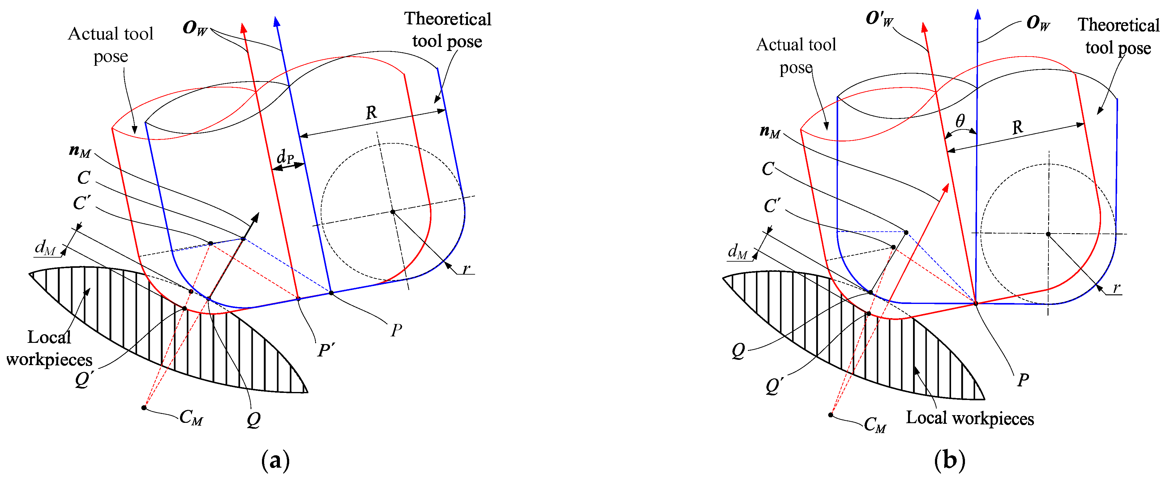
In essence, the goal of tool position planning in overall machining is to ensure that the final tool envelope surface closely approximates the design surface of the blade. However, the tool envelope surface is only finalized after all tool positions have been determined, which complicates the optimization of tool positions. The theoretical machining error is the deviation between the design surface and the tool envelope surface. During machining, the permissible machining deviation is minimal compared to the minimum radius of curvature of the cutting edge’s rotating surface. Consequently, the machining deviation can be represented by the overcutting or undercutting depth at the theoretical tangential contact point on the machined surface, as illustrated in Figure 8. In the theoretical tool position, the rotary surface of the cutting edge of the tool is tangent to the workpiece surface at the tangent contact point Q. And the vector nM represents the unit external normal vector of the machined surface at the theoretical tangent contact, while point C denotes the center of the circle of the rounded cutting edge. When the tip point transitions from the theoretical position P to the deviated position P’, the cutting edge of the tool also shifts in space, represented by the vector nP. In contrast, under the influence of tool axis deviation, the tool axis vector is rotated from its theoretical position OW to the deviated position OW. Consequently, the cutting edge of the tool also rotates around the tip point in space. The angle between the unit vectors OW and OW is denoted as θ.
The tool tip point deviation can be decomposed into a movement along the direction of vector nM and a movement in the normal plane at the tangential contact point, as illustrated in Figure 8a. The displacement ln along the direction of vector nM results in the tool either cutting into or moving away from the machined surface, while the displacement lm in the normal plane at the tangent point causes the tool to deviate from the theoretical tangent point. The lengths ln and lm can be calculated using Equation (8).
l n = Δ P W n M , l m = Δ P W sin < Δ P W , n M >
Relative to the radius of curvature of the machined surface at the point of tangential contact, the difference in chord height that occurs after the cutting edge moves a distance of lm in the tangent plane at this contact point is minimal. Consequently, the machining deviation generated by the tool moving along the direction mM can be considered negligible. The machining error lP, resulting from the deviation of the tool tip point, is equivalent to the distance ln, expressed as lP = ln. Specifically, when lP > 0, theoretical undercutting occurs at the tangential contact; conversely, when lP < 0, theoretical overcutting occurs at the tangential contact.
Similar to the tip deviation of the tool, the vector deviation of the tool axis will also alter the meshing relationship between the rotary surface of the cutting edge of the tool and the machined curved surface, thereby causing overcutting or undercutting at the theoretical tangent point, as illustrated in Figure 8b. The plane defined by vector OW and vector nM is denoted as πM, with its normal vector represented by tM. And the plane perpendicular to both plane πM and vector nM is denoted as πM, with its normal vector represented by tm. Then the vectors tM and tm can be derived from Equation (9).
t M = O W × n M ,   t m = t M × n M
Unlike the translational movement of the cutting edge of a tool along the tip point, the vector deviation of the tool axis causes the surface of the cutting edge at the contact point to experience both rotational and translational displacements simultaneously. The rotated position of the center point C of the circle is denoted as point C′, while the directed distance from point C to point C′ is represented by the vector nω. Therefore, the process of movement of the cutting edge surface of the tool under the action of the vector deviation of the tool axis can be divided into first moving along the vector nω and then rotating by an angle θ about the vector tω passing through the point C′. Since the generatrix of the cutting edge rotation of the tool is an arc, when the tool rotates around the center point C of the arc, the relative positional relationship between the tool and the machined surface remains unchanged. Consequently, the projection of the tool along vector nω onto the normal vector nM represents the overcut or undercut amount dM of the cutting edge at the contact point Q.
The plane of rotation defined by vector OW and OW is denoted as πω when the tool axis vector is adjusted from OW and OW. The direction of rotation, represented by the normal vector to this plane, is denoted as tω. Consequently, the vector tω and the angle θ are calculated according to Equation (10).
t ω = O W × O W ,   θ = arccos < O W O W >
Furthermore, the vector nω from point C to point C′ can be calculated from Equation (11).
n ω = C M C 1 cos θ sin θ 0 sin θ cos θ 0 0 0 1 M C C
where MC is the rotation matrix when the point C′ revolves around the vector tω, and MC−1 is the inverse of the matrix MC.
M C = O W , t ω , O W × t ω
Therefore, the directed distance lθ by which the tool moves in the direction of the vector nM can be calculated from Equation (13).
l θ = n ω n M
Thus, under the combined effect of cutter tip point deviation and cutter axis vector deviation, the maximum overcut depth or minimum undercut thickness dM at the theoretical cutting contact point can be calculated by Equation (14). Here, lP and lθ are algebraic values and independent of each other, so the combined effect of cutter tip point deviation and cutter axis vector deviation may either have an additive effect or offset each other.
d M = l P + l θ
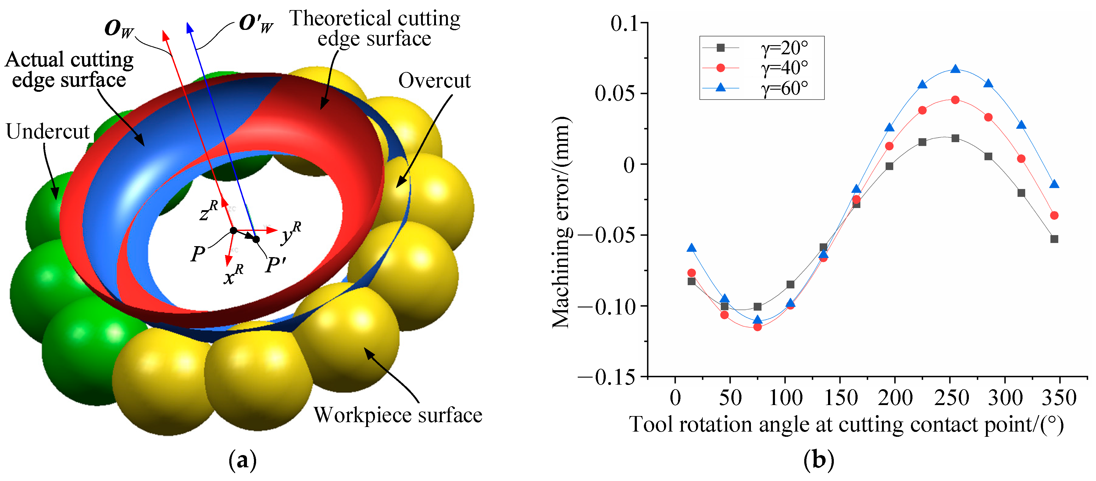
It should be noted that in Equation (14), lP and lθ are independent of each other and each can be either positive or negative. Therefore, the combined effect of cutter tip point deviation and cutter axis vector deviation may either amplify or cancel each other out, depending on the direction of deviation, as illustrated in Figure 9a. Figure 9b presents the distribution of machining errors along the cutting contact point positions under the condition of cutter tip point deviation ΔPW = [0.1, 0.1, 0.1]Tand cutter axis vector deviation ΔOW = [0.0, 0.99999, −0.00436]T for different tool rake angles. In Figure 9b, the tool rake angle γ is defined as the angle between the cutter axis vector O (aligned with the positive zR axis direction in Figure 9a) and the normal vector, while the circumferential angle refers to the angle between the projection vector of the normal vector nM in the xR-yR plane and the positive xR axis. As observed in Figure 9b, under identical cutter tip point deviation and cutter axis vector deviation, the machining error at the cutting contact point on the machined surface varies with the position of the cutting contact point on the tool’s rotational surface. Furthermore, the depth of overcutting or undercutting at the cutting contact point differs based on the location of the cutting contact point on the tool’s rotational surface.

3.2. Optimal Cutter Location Point Search Algorithm

The linear path in five-axis machining is obtained through linear interpolation of the theoretical curved path. Shorter interpolation segments yield higher approximation accuracy but exponentially increase the number of path segments. Moreover, excessively short linear paths require frequent acceleration/deceleration of the machine tool during CNC execution, which not only reduces machining efficiency but also degrades machining quality due to prolonged dwell time at corner points. Therefore, this section aims to maximize interpolation segment length under machining error constraints while determining optimal cutter location points and concurrently establishes the upper limit for transition errors at linear path corners. The process of searching for optimal endpoints of linear interpolation paths along synchronized motion trajectories of linear and rotary axes involves three steps. Firstly, calculate the maximum deviation in motion trajectories of linear and rotary axes corresponding to the current search step length. Subsequently, estimate the upper bound of machining error. Finally, adjust the search step length based on the discrepancy between the estimated error upper bound and the maximum permissible error. Notably, when searching endpoints for the first two linear paths, only machining errors induced by linear interpolation are considered.
For complex machine tool motion trajectories, the curved paths corresponding to linear path segments may include arc-shaped and S-shaped forms, as illustrated in Figure 10. During optimal cutter location point searches, path classification must precede analysis. If dealing with an arc-shaped curve segment, the upper bound of machining error on the current linear path can be directly estimated. Otherwise, the segment should be divided into two arc-shaped curve segments, with their respective machining error upper bounds estimated separately. The classification criterion depends on the sagitta distribution: if the interpolated curve segment exhibits only one local maximum sagitta value, it is arc-shaped; otherwise, it is S-shaped. Moreover, the point where sagitta equals zero serves as the demarcation point between two adjacent arc-shaped curve segments.
Based on the preceding analysis, Figure 11 presents the flowchart of the curve parameter search algorithm for optimal cutter location points under constant tolerance constraints. When implementing the search algorithm shown in Figure 11, the input parameters include synchronized motion trajectory curves for machine tool linear axes and rotary axes CT(v) and CR(v), maximum permissible machining error [dM], adjacent search step resolution [Δv], and initial corner transition thresholds [εm,T] = 0 and [εm,R] = 0. The algorithm outputs the number of ordered linear path segments Nv, the curve parameter vi at the terminal endpoint of the i-th linear path segment, and the maximum allowable thresholds for linear interpolation path [εm,T] and [εm,R]. During the optimal cutter location point search process, the average of maximum deviations in motion trajectories along the first two linear paths is set as the initial threshold for linear paths. Starting from the third linear path endpoint search, machining errors from both linear interpolation and corner transitions are evaluated simultaneously. Moreover, when the latter exceeds the former, it is necessary to reduce thresholds at corner transition paths and recalculate the machining error upper bound. By means of this algorithm, linear interpolation paths with minimal redundant points can be obtained, and machining errors are maintained within constrained tolerance limits.

4. Application Verification and Discussion

4.1. Example and Comparative Analysis

In this subsection, the optimal cutter location point search algorithm under constant machining error constraints is compared with the traditional cutter tip sagitta-constrained discretization algorithm using a fan blisk blade’s five-axis spiral machining toolpath as the application object, with verification conducted from two aspects: the number of obtained cutter location points and the uniformity of maximum machining error values across linear path segments. The five-axis machining of large fan blisk blade surfaces employs spiral continuous milling around the blade stacking axis. Within each cyclic cutting unit of the fan blisk’s five-axis spiral milling process, the tool must traverse the leading/trailing edge regions and pressure/suction side regions, thereby reflecting the characteristics of both the toolpath and rotary axis movements during five-axis machining.
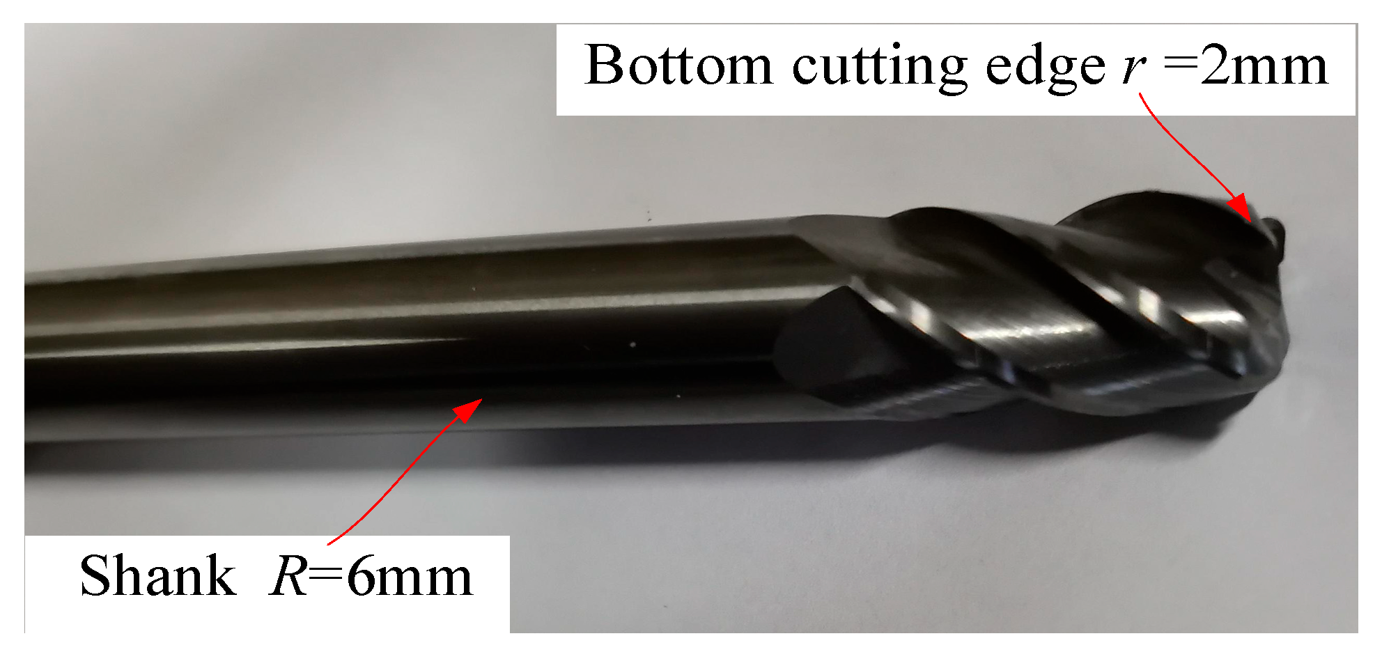
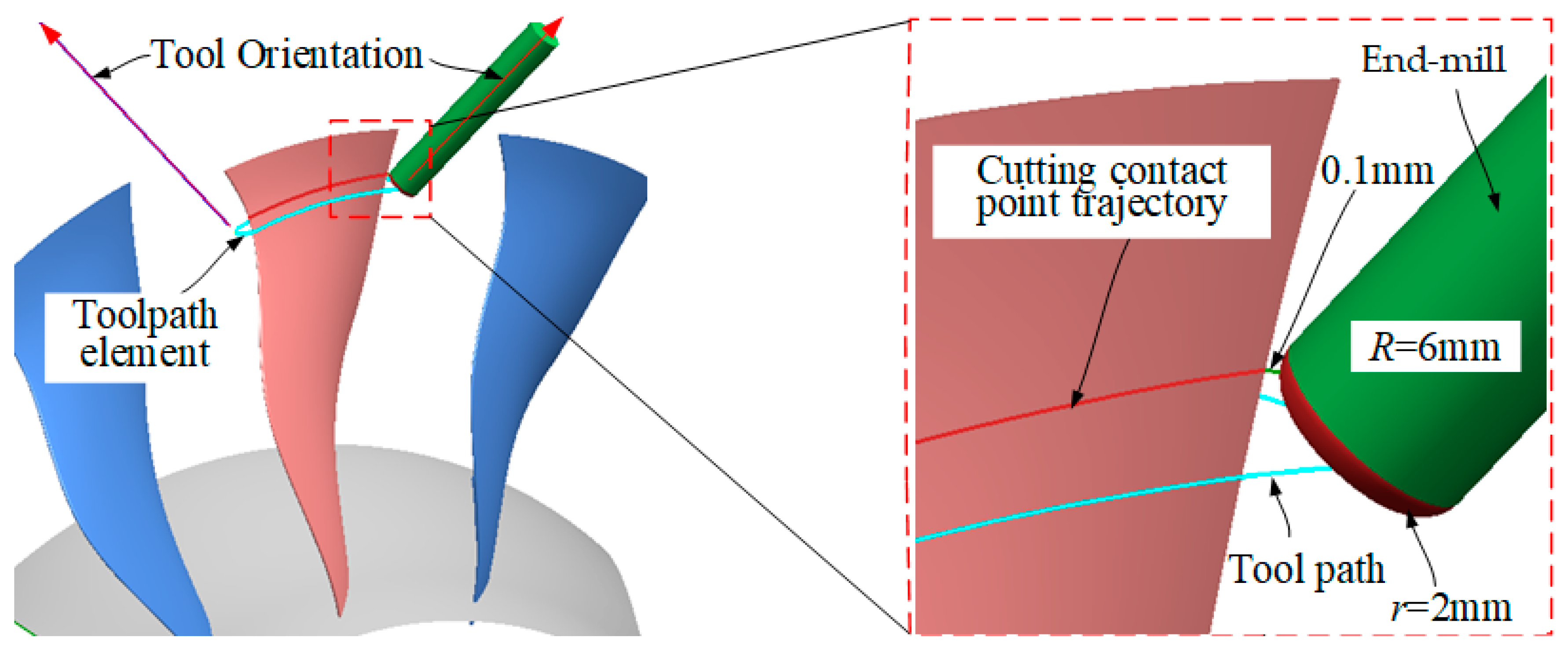
The fan blisk structure is identical to that shown in Figure 1. Its outer hub diameter is approximately 803.0 mm, while the inner hub diameter ranges between 477.2 mm and 523.2 mm. The blade surfaces are free-form surfaces, with a maximum length of approximately 163.0 mm and a width of about 112.5 mm. Additionally, the maximum blade thickness is 4.35 mm, while the minimum radius of curvature in the leading and trailing edge regions is 0.176 mm. The material of the fan blisk is titanium alloy TC4. To reduce vibration and deformation during the machining process, the prebliskion machining of blades is divided into two stages: semi-finishing and finishing. During the semi-finishing and finishing of blade of fan blisk, a hard alloy toroidal end-mill cutter with shank radius R = 6 mm and bottom cutting edge radius r = 2 mm is used, as shown in Figure 12. The cutter is purchased from Zhuzhou Diamond Cutting Tools Co., Ltd. in Zhuzhou, China. Without loss of generality, the toolpath element position selected for the semi-finishing stage of the blade surface is shown in Figure 13. And the permissible machining error upper limit is set as 0.04 mm, and the allowance of 0.1 mm is reserved for subsequent prebliskion finishing.
Based on the UG NX10 CAD/CAM platform, the theoretical cutting contact point trajectory is extracted from the blade surface, and then a cutter tip trajectory and appropriate cutter axis orientation are constructed with a 0.1 mm machining allowance, where the cutter tip trajectory length measures 209.763 mm. Then, based on the algorithm proposed in this work, a corresponding plug-in was developed to perform linear interpolation with equivalent theoretical machining error compensation and associated post-processing. On this obtained cutter tip trajectory curve, discrete cutter location points for linear interpolation paths are sequentially searched using both the method proposed in this section and the constant chord height tolerance method for cutter tip linear segments in the workpiece coordinate system, ultimately generating a cutter location file. The constant machining tolerance constraint algorithm yields 127 discrete cutter location points. Due to the non-corresponding relationship between machining error and chord height deviation in the traditional chord height tolerance-based linear interpolation method under the workpiece coordinate system, after multiple tests, the chord height tolerance is set to 0.025 mm, resulting in a maximum machining deviation of 0.038 mm on linear paths. At this setting, 235 discrete cutter location points are generated along the cutter tip trajectory. Compared with the constant chord height control method, the tool position redundancy obtained by the constant machining error constraint method is markedly reduced, with the number of tool position points per single cutting unit decreased by approximately 45.9%.
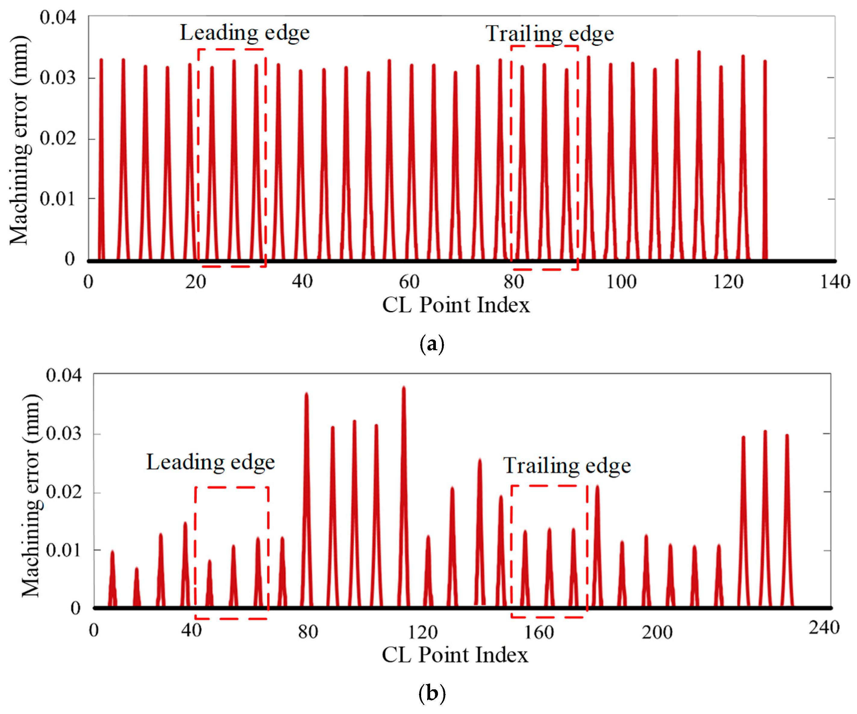
The statistical results of maximum machining deviations across linear interpolation path segments obtained by the above two methods are presented in Figure 14, where, for enhanced clarity, Figure 14a displays maximum values taken over every five adjacent cutter location points, while Figure 14b shows the maxima calculated over every ten adjacent cutter location points. As observed in Figure 14a, the maximum machining errors along linear paths corresponding to discrete cutter location points generated via the constant machining error constraint method are primarily distributed within a narrow range of 0.031 mm~0.034 mm with deviation uniformity, specifically showing minimum machining error at 77.5% of theoretical maximum error and maximum machining error at 85% of the theoretical maximum error. The failure to achieve theoretical error limits stems from conservative estimations during computation: conservative conversion from machine tool linear/rotary axis motion deviations to cutter tip/axis deviations and conservative estimation when calculating maximum machining errors on linear paths based on tool pose deviations. However, the deviations between maximum machining errors on each linear path generated by the constant chord height tolerance constraint method and theoretical values are more significant. As observed in Figure 14b, maximum machining errors across linear paths are distributed within the range of 0.007 mm~0.038 mm, where the minimum machining error on paths is only 17.5% of the theoretical maximum error while the maximum machining error reaches 95% of the theoretical maximum error. This dispersion of maximum machining errors stems from the fact that machining errors induced by cutter tip deviation and cutter axis deviation may act either in the same direction or opposite directions: when error directions coincide, the maximum deviation on linear paths increases, whereas when directions oppose, the deviation decreases. Against the baseline constant chord height control, the constant machining error constraint strategy enhances the consistency of theoretical machining errors at tool position points. Specifically, the error fluctuation band narrows from an initial 17.5%~95% amplitude to a controlled 77.5%~85% band.

4.2. Applications and Comparisons

Building upon the semi-finishing stage, a cutter tip trajectory and appropriate cutter axis orientation for prebliskion five-axis milling of the blisk blade are constructed with zero machining allowance. With the maximum machining error set at 0.002 mm, linear interpolation and post-processing are performed using both constant machining error constraints and constant chord height tolerance constraints. The linear path cutter location file obtained from post-processing undergoes machine-specific post-processing according to the machine tool structure and CNC system model to generate formatted NC programs for machining. Given identical geometric configurations across all blades of the blisk, a single-blade trial machining is conducted.
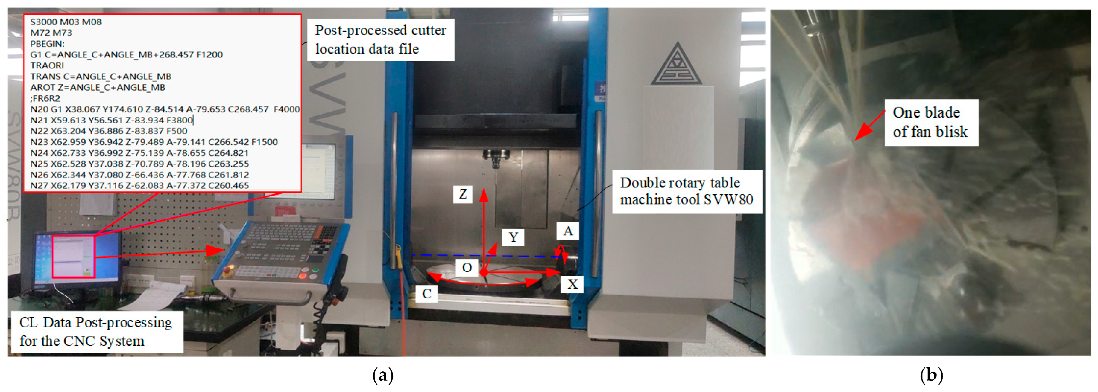
During the experimental process, the dual-turntable five-axis machine tool SVW80 equipped with the Siemens 840Dsl CNC system was used as the experimental research platform. The machine tool SVW80 is purchased from Dalian Sanlei Machine Co., Ltd. in Dalian, China. The process of prebliskion machining of the blisk blade is illustrated in Figure 15. In the prebliskion machining process of integral blisk blades, cutting begins at the junction of the trailing edge surface and the disk surface, utilizing a helical milling path around the blade; furthermore, based on the author’s prior research, machining parameters must be individually set based on location, specifically adjusting spindle speed and tool feed rate, where for machining the trailing edge and leading edge regions, the spindle speed is set to a constant 8000 r/min and the tool feed rate is held constant at 1500 mm/min, whereas for machining the pressure surface and suction surface regions of blade, the spindle speed is set to a constant 15,000 r/min and the tool feed rate is held constant at 4500 mm/min, with linear interpolation applied between different regions to achieve a smooth transition.
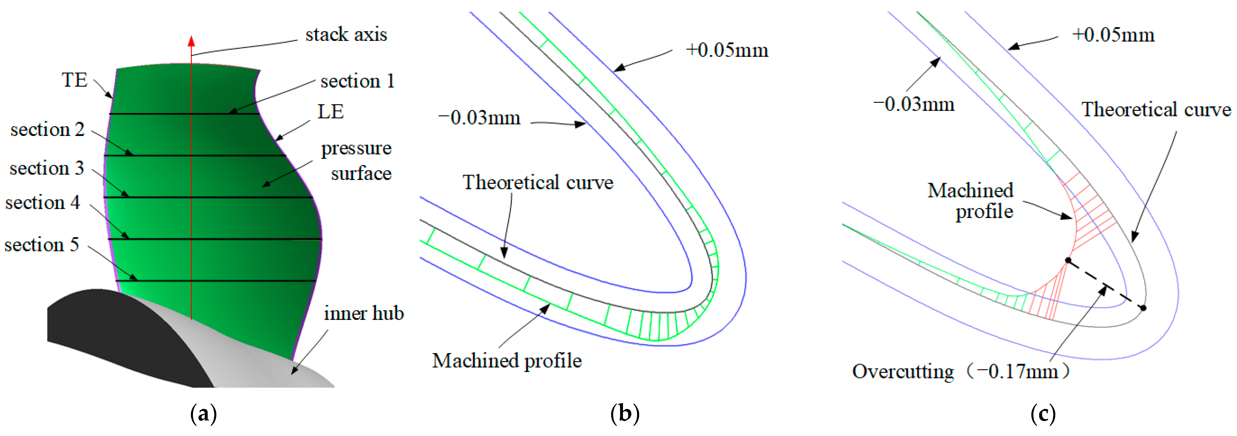
To compare the differences between the two methods, a coordinate measuring machine (CMM) was employed to obtain cross-sectional profile data of the blisk blades at uniform height intervals. The five theoretical curves are extracted from the sections perpendicular to the stack axis on the blade, as shown in Figure 16. The collected data is processed using specialized blade analysis software PC-DMIS CAD++ V1.0 to calculate deviations at each corresponding location. The evaluation of the constant-height section profiles of the blade surface involves comparing the actual contour curve against the theoretical curve. Since standard data processing methods and specialized software exist for this purpose, we do not elaborate further here. The machining defects are more likely to occur in the regions of the LE due to severe distortion and drastic curvature changes. As observed in Figure 16, the NC program employing linear interpolation with constant machining error constraints produces a more complete leading edge contour profile of the integral blade, ensuring machining accuracy even at small curvature radii. The machining error for the constant-height cross-sectional contour in the blade leading edge region ranges from −0.03 mm to +0.05 mm, meeting application requirements, as shown in Figure 16b. In contrast, the program using linear interpolation with constant chord height tolerance exhibits significant contour deviations on the machined blade leading edge. The machining error of the constant-height cross-sectional contour in the blade leading edge region exceeds the acceptable range of −0.03 mm to +0.05 mm, with a maximum overcut reaching −0.17 mm, which fails to meet application requirements, as shown in Figure 16c. This occurs because five-axis machining of blade leading/trailing edge regions requires rapid responses from both linear and rotary axes during drastic tool motion changes. Under such conditions, the chord height tolerance method generates excessive redundant cutter location points to maintain interpolation accuracy, exacerbating frequent machine acceleration/deceleration cycles and reducing effective feed per tooth at the cutting edge. Concurrently, the poor rigidity of blisk blades in cantilever machining states induces tool deflection and vibration on machined surfaces, consequently resulting in contour distortion.
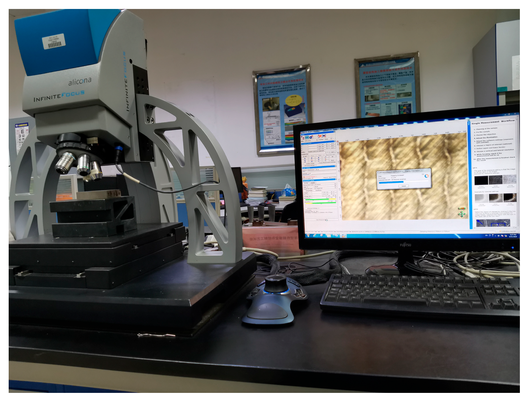
The surface topography of the machined blades was measured using an Alicona automated tool measuring instrument, as shown in Figure 17. Correspondingly, the surface quality comparison of the leading edge region on blisk blade specimens machined using the two respective programs is presented in Figure 18. As observed in Figure 18, compared to the tool interpolation program employing constant chord height tolerance constraints, the machining program implementing interpolation with constant machining error constraints achieves superior surface quality. This occurs because during leading edge machining, the workpiece exhibits minimum rigidity where frequent acceleration/deceleration readily induces chatter, consequently degrading surface quality. Comprehensive comparison confirms that for both contour geometry and surface quality in the blisk blade leading edge region, linear interpolation via constant machining error constraints reduces cutter location point redundancy, increases machine tool motion speed, minimizes frequent acceleration/deceleration, and ultimately enhances the overall surface machining quality of blisk blades.

5. Conclusions

Focused on linear interpolation in five-axis toolpaths for blisk blade surfaces, this paper establishes a computational scheme for generating prebliskion-constrained tool position points. The principal findings are summarized as follows:
  • Based on the machine tool kinematic model, a mapping relationship is established between machine tool trajectory deviations and tool pose deviations. This enables the calculation method for maximum overcut/undercut induced by coupled deviations of tool tip position and tool orientation. Building upon this foundation, a linear interpolation tool position point search algorithm with constant theoretical machining error constraints is developed.
  • During linear interpolation of complex tool motion trajectories in five-axis machining of blisk blades, compared with the constant chord height control method, the constant machining theoretical error constraint method significantly reduces tool position point redundancy while substantially improving uniformity in theoretical machining error distribution. Specifically, the number of tool position points of the cutting unit decreases by approximately 45.9%, and the machining error fluctuation range narrows from 17.5%~95% to 77.5%~85%.
  • Machining tests on blisk blade specimens demonstrate that in the leading edge region, where abrupt variations occur in both tool tip position and tool axis orientation, the constant machining theoretical error constraint method generates more rational distributions of tool position points. This approach minimizes frequent machine tool acceleration/deceleration, thereby optimizing contour fidelity and enhancing surface quality.

Author Contributions

Conceptualization, Z.W. and H.W.; data curation, Z.W. and S.M.; formal analysis, Z.S. and H.W.; funding acquisition, Z.W.; investigation, Z.W., S.M. and H.W.; methodology, Y.T. and H.W.; project administration, Z.W. and H.W.; resources, Z.W.; software, S.M. and Z.S.; supervision, H.W.; validation, Y.T. and S.M.; writing—original draft, Z.W. and Z.S.; writing—review and editing, Z.W., Z.S. and Y.T. All authors have read and agreed to the published version of the manuscript.

Funding

This study was supported by the National Natural Science Foundation of China (No. 91960203 and No. 52105182).

Data Availability Statement

The data used to support the findings of this study are available from the corresponding author upon request.

Conflicts of Interest

Author Shuanglong Mao was employed by Aecc South Industry Company Limited. The remaining authors declare that the research was conducted in the absence of any commercial or financial relationships that could be construed as a potential conflict of interest.

References

  1. Wang, Z.; Lin, X.; Shi, Y.; Chen, Z. Reducing roughness of freeform surface through tool orientation optimization in multi-axis polishing of blisk. Int. J. Adv. Manuf. Technol. 2020, 108, 917–929. [Google Scholar] [CrossRef]
  2. Wang, Z.; Lin, X.; Shi, Y. Efficiently constructing collision-free regions of tool orientations for holder in five-Axis machining of Blisk. Chin. J. Aeronaut. 2020, 33, 2743–2756. [Google Scholar] [CrossRef]
  3. Wang, Z.; Lin, X.; Shan, C.; Tian, H. Reducing the contour error of leading and trailing edge through feedrate scheduling in axis machining of blisk. Int. J. Adv. Manuf. Technol. 2024, 134, 4887–4905. [Google Scholar] [CrossRef]
  4. Yuen, A.; Zhang, K.; Altintas, Y. Smooth trajectory generation for five-axis machine tools. Int. J. Mach. Tools Manuf. 2013, 71, 11–19. [Google Scholar] [CrossRef]
  5. Zhang, J.; Mo, R.; Wan, N.; Xia, C. Tool path planning for five-axis flank milling of free-form surfaces. Int. J. Adv. Manuf. Technol. 2020, 108, 73–90. [Google Scholar] [CrossRef]
  6. Yan, B.; Hao, Y.; Zhu, L.; Wang, Z.; Li, Y.; Chen, J. Towards high milling accuracy of turbine blades: A review. Mech. Syst. Signal Process 2022, 170, 108727. [Google Scholar] [CrossRef]
  7. Zhou, Y.; Jiang, Y.; Lu, C.; Huang, J.; Pei, J.; Xing, T.; Zhao, S.; Zhu, K.; Yan, H.; Xu, Z.; et al. A review of 5-axis milling techniques for centrifugal impellers: Tool-path generation and deformation control. J. Manuf. Process 2024, 131, 160–186. [Google Scholar] [CrossRef]
  8. Lasemi, A.; Xue, D.; Gu, P. Recent development in CNC machining of freeform surfaces: A state-of-the-art review. Comput. Aided Des. 2010, 42, 641–654. [Google Scholar] [CrossRef]
  9. Liang, F.; Kang, C.; Fang, F. A review on tool orientation planning in multi-Axis machining. Int. J. Prod. Res. 2020, 59, 5690–5720. [Google Scholar] [CrossRef]
  10. Jiang, X.; Zhang, Y.; Li, Y.; He, J.; Zhang, X. Critical geometric errors identification of a five-Axis machine tool based on global quantitative sensitivity analysis. Int. J. Adv. Manuf. Technol. 2022, 119, 3717–3727. [Google Scholar] [CrossRef]
  11. Chen, Q.; Zhang, Y.; Li, X.; He, J.; Xu, X. Separation and compensation of geometric errors of rotary axis in 5-axis ultra-prebliskion machine tool by empirical mode decomposition method. J. Manuf. Process 2021, 68, 1509–1523. [Google Scholar] [CrossRef]
  12. Wu, L.; Xu, J.; Xing, H.; Sun, Y. Accurate detection and smoothness-oriented avoidance method of singularity in axis CNC machining. Comput. Aided Des. 2024, 167, 103652. [Google Scholar] [CrossRef]
  13. Xiao, J.; Fang, J.; Li, B.; Zhang, H. Dynamic velocity planning method for parametric toolpath with mode-based tracking error control. Int. J. Adv. Manuf. Technol. 2023, 128, 4804817. [Google Scholar] [CrossRef]
  14. Ni, Y.; Liu, X.; Zhang, B.; Zhang, Z.; Li, J. Geometric error measurement and identification for rotational axes of a five-axis CNC machine tool. J. Mech. Eng. 2018, 64, 290–302. [Google Scholar]
  15. Rahaman, M.; Seethaler, R.; Yellowley, I. A new approach to contour error control in high speed machining. Int. J. Mach. Tools Manuf. 2015, 88, 42–50. [Google Scholar] [CrossRef]
  16. Huang, J.; Du, X.; Zhu, L. Real-time local smoothing for five-axis linear toolpath considering smoothing error constraints. Int. J. Mach. Tools Manuf. 2018, 124, 67–79. [Google Scholar] [CrossRef]
  17. Lu, Y.; Ding, Y.; Wang, C.; Zhu, L. Tool path generation for five-axis machining of blisks with barrel cutters. Int. J. Prod. Res. 2018, 57, 1300–1314. [Google Scholar] [CrossRef]
  18. Xu, J.; Zhang, D.; Sun, Y. Kinematics performance oriented smoothing method to plan tool orientations for axis ball-end CNC machining. Int. J. Mech. Sci. 2019, 157–158, 293–303. [Google Scholar] [CrossRef]
  19. He, D.; Li, Z.; Li, Y.; Tang, K. Quasi-developable and signed multi-strip approximation of a freeform surface mesh for efficient flank milling. Comput.-Aided Des. 2021, 140, 103083. [Google Scholar] [CrossRef]
  20. Bi, Q.; Shi, J.; Wang, Y.; Zhu, L.; Ding, H. Analytical curvature-continuous dual-Bézier corner transition for five-axis linear tool path. Int. J. Mach. Tools Manuf. 2015, 91, 96–108. [Google Scholar] [CrossRef]
  21. Chu, M.; Bohez, A.; Erik, L. A novel differential kinematics model to compare the kinematic performances of axis CNC machines. Int. J. Mech. Sci. 2019, 163, 105117. [Google Scholar] [CrossRef]
  22. Guo, Y.; Niu, W.; Zhou, J.; Liu, H. Near-time optimal feedrate planning for the NURBS curve considering interpolation error constraints. Rob. Comput. Integr. Manuf. 2024, 86, 102679. [Google Scholar] [CrossRef]
  23. Yan, Y.; Zhang, L.; Gao, J. Tool path planning for flank milling of non-developable ruled surface based on immune particle swarm optimization algorithm. Int. J. Adv. Manuf. Technol. 2021, 115, 1063–1074. [Google Scholar] [CrossRef]
  24. Fan, J.; Zhang, Y. A novel methodology for predicting and identifying geometric errors of rotary Axis in five-Axis machine tools. Int. J. Adv. Manuf. Technol. 2020, 108, 2255–2265. [Google Scholar] [CrossRef]
  25. Li, D.; Zhang, W.; Zhou, W.; Shang, T.; Fleischer, J. Dual NURBS path smoothing for 5-axis linear path of flank milling. Int. J. Preblisk Eng. Manuf. 2018, 19, 1811–1820. [Google Scholar] [CrossRef]
  26. Rajain, K.; Sliusarenko Oleksii, S.; Bizzarri, M.; Barton, M. Curve-guided 5-axis CNC flank milling of free-form surfaces using custom-shaped tools. Comput. Aided Geom. D 2022, 94, 102082. [Google Scholar] [CrossRef]
  27. Arai, W.; Tanaka, F.; Onosato, M. Error estimation of machined surfaces in multi-axis machining with machine tool errors including tool self-intersecting motion based on high-accuracy tool swept volumes. Int. J. Autom. Technol. 2018, 12, 680–687. [Google Scholar] [CrossRef]
  28. Tulsyan, S.; Altintas, Y. Local toolpath smoothing for five-axis machine tools. Int. J. Mach. Tools Manuf. 2015, 96, 126. [Google Scholar] [CrossRef]
  29. Yang, J.; Yuen, A. An analytical local corner smoothing algorithm for five-axis CNC machining. Int. J. Mach. Tools Manuf. 2017, 123, 22–35. [Google Scholar] [CrossRef]
  30. Cripps, R.; Cross, B.; Hunt, M.; Mullineux, G. Singularities in five-axis machining cause, effect and avoidance. Int. J. Mach. Tools Manuf. 2017, 116, 40–51. [Google Scholar] [CrossRef]
  31. Sun, Y.; Jia, J.; Xu, J.; Chen, M.; Niu, J. Path, feedrate and trajectory planning for free-form surface machining: A state-of-the-art review. Chin. J. Aeronaut. 2022, 35, 18. [Google Scholar] [CrossRef]
  32. Sun, Y.; Chen, M.; Jia, J.; Lee, Y.; Guo, D. Jerk-limited feedrate scheduling and optimization for five-axis machining using new piecewise linear programming approach. Sci. China Technol. Sc. 2019, 62, 5–19. [Google Scholar] [CrossRef]
  33. Sun, S.; Sun, Y.; Xu, J. Tool path generation for axis flank milling of ruled surfaces with optimal cutter locations considering multiple geometric constraints. Chin. J. Aeronaut. 2023, 36, 408–424. [Google Scholar] [CrossRef]
  34. Lu, Z.; Huo, G.; Jiang, X. A novel method to minimize the five-axis CNC machining error around singular points based on closed-loop inverse kinematics. Int. J. Adv. Manuf. Technol. 2023, 128, 2237–2249. [Google Scholar] [CrossRef]
  35. Cong, H.; Zha, J.; Chen, Y. Efficient compensation method of 5-axis machine tools based on a novel representation of the volumetric error. Int. J. Adv. Manuf. Technol. 2023, 126, 1109–1119. [Google Scholar] [CrossRef]
  36. Tajima, S.; Sencer, B. Online interpolation of 5-axis machining toolpaths with global blending. Int. J. Mach. Tools Manuf. 2022, 175, 103862. [Google Scholar] [CrossRef]
  37. Hu, Y.; Jiang, X.; Huo, G.; Su, C.; Zhou, S.; Wang, B.; Li, H.; Zheng, Z. A novel feed rate scheduling method with acc-jerk-continuity and round-off error elimination for non-uniform rational B-spline interpolation. J. Comput. Des. Eng. 2023, 10, 294–317. [Google Scholar] [CrossRef]
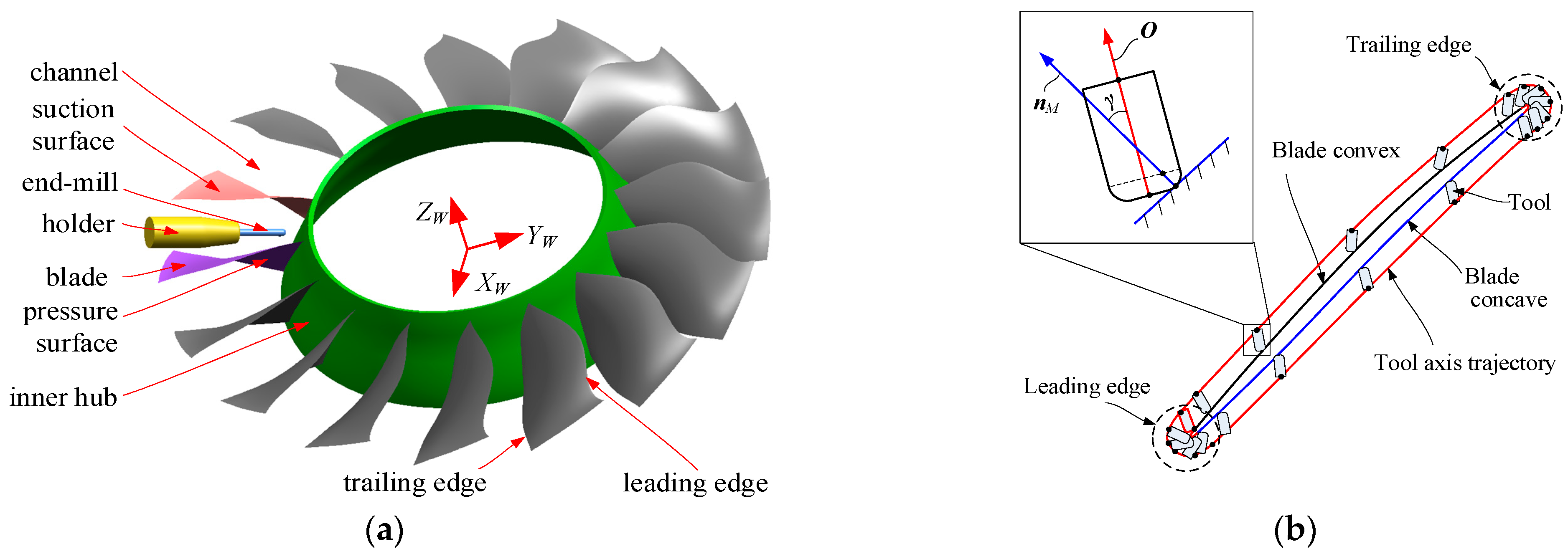
Figure 1. Toolpath for 5-axis spiral machining of fan blisk. (a) Geometric structure feature. (b) Theoretical toolpath of end-mill cutter.
Machines 13 00768 g001
Figure 2. Tool linear interpolation path and CNC machine tool motion.
Machines 13 00768 g002
Figure 3. Linear interpolation of theoretical tool trajectory in 5-axis machining of complex surfaces.
Machines 13 00768 g003
Figure 4. Five-axis machining linear interpolation and path transfer fairing theoretical error with end-mill cutter.
Machines 13 00768 g004
Figure 5. Deviation of line interpolation path in machine tool coordinate system. (a) Three-dimensional trajectory curve of the linear axis. (b) Two-dimensional trajectory curve of the axis of rotation.
Machines 13 00768 g005
Figure 6. Deviation of curve path and linear interpolation.
Machines 13 00768 g006
Figure 7. The influence of end-mill tool pose deviation on the position of rotary surface of cutting edge. (a) Tool movement. (b) Tool tip deviation. (c) Tool axis deviation.
Machines 13 00768 g007
Figure 8. Theoretical machining error caused by end-mill cutter position and pose deviation. (a) Tool tip deviation. (b) Tool axis deviation.
Machines 13 00768 g008
Figure 9. The distribution of machining error with the position of tangent contact. (a) Schematic diagram of tool pose deviation. (b) Machining error distribution.
Machines 13 00768 g009
Figure 10. Deviation of machine tool motion trajectories on the two curve segments. (a) Arc-shaped curve segment. (b) S-shaped curve segment.
Machines 13 00768 g010
Figure 11. Flowchart of curve parameter algorithm at linear path endpoints.
Machines 13 00768 g011
Figure 12. Toroidal end-mill cutter used in 5-axis helical machining of fan blisk.
Machines 13 00768 g012
Figure 13. Toolpath element for 5-axis helical machining of fan blisk.
Machines 13 00768 g013
Figure 14. Machining error distribution comparison of different linear path methods. (a) Constant machining error constraints. (b) Constant chord height deviation constraints.
Machines 13 00768 g014
Figure 15. Prebliskion machining of test specimen of blisk blade. (a) Five-axis machine tool for specimen machining. (b) Processing process.
Machines 13 00768 g015
Figure 16. Cross-sectional contour comparison of leading edge region on test specimen of blisk blade. (a) CMM measurement planning of blisk blade. (b) Constant machining error constraints. (c) Constant chord height deviation constraints.
Machines 13 00768 g016
Figure 17. Surface topography measurement of machined surface of fan blisk blade.
Machines 13 00768 g017
Figure 18. Surface quality comparison of two interpolation methods. (a) Constant machining error constraints. (b) Constant chord height deviation constraints.
Machines 13 00768 g018
Disclaimer/Publisher’s Note: The statements, opinions and data contained in all publications are solely those of the individual author(s) and contributor(s) and not of MDPI and/or the editor(s). MDPI and/or the editor(s) disclaim responsibility for any injury to people or property resulting from any ideas, methods, instructions or products referred to in the content.