Six-Dimensional Spatial Dimension Chain Modeling via Transfer Matrix Method with Coupled Form Error Distributions

Abstract

In tolerance design for complex mechanical systems, 3D dimension chain analyses are crucial for assembly accuracy. The current methods (e.g., worst-case analysis, statistical tolerance analysis) face limitations from oversimplified assumptions—treating datum features as ideal geometries while ignoring manufacturing-induced spatial distribution of form errors and failing to characterize 3D coupled error constraints. This study proposes a six-dimensional spatial dimension chain (SDC) model based on transfer matrix theory. The key innovations include (1) a six-dimensional model integrating position and orientation vectors, incorporating geometric error propagation constraints for high-fidelity error prediction and tolerance optimization, (2) the characterization of spatially distributed form errors and 3D coupled errors of spatial dimension chain-based multiple mating-surface constraint (SDC-MMSC) using six-degree-of-freedom (6-DoF) geometric error components, reducing the assembly topology complexity while improving the efficiency, and (3) a 6-DoF error characterization method for non-mating-constrained data, providing the theoretical basis for SDC modeling. The experimental validation on an aero-engine casing assembly shows that the SDC model captures multidimensional closed-loop spatial errors, with absolute errors of max–min closed-loop distances below 9.3 μm and coaxiality prediction errors under 8.3%. The SDC-MMSC method demonstrates superiority, yielding normal vector angular errors <0.008° and envelope surface RMSE values <0.006 mm. This method overcomes traditional simplified assumptions, establishing a high-precision, multidimensional distributed-form-error-driven SDC model for complex mechanical systems.

1. Introduction

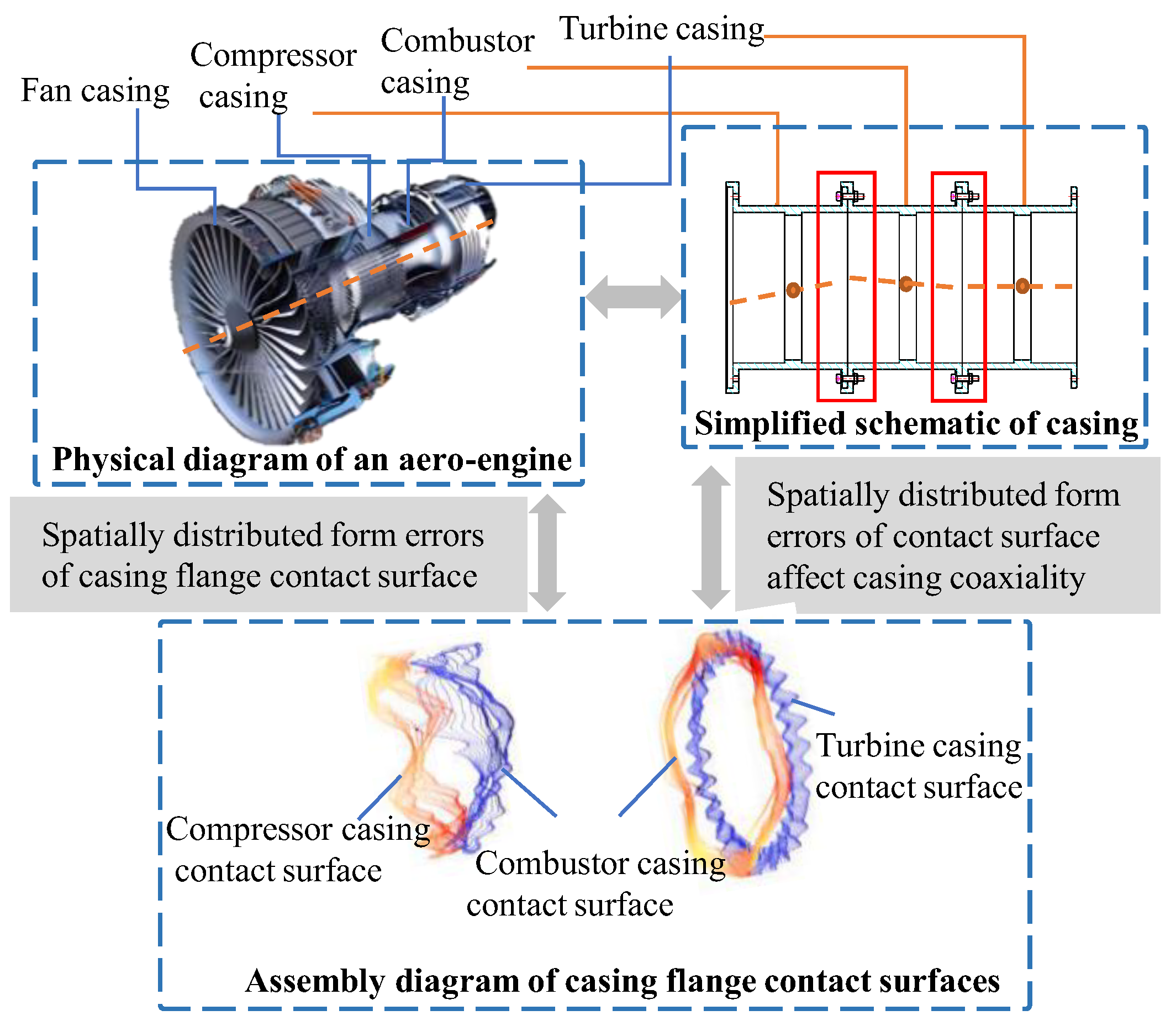
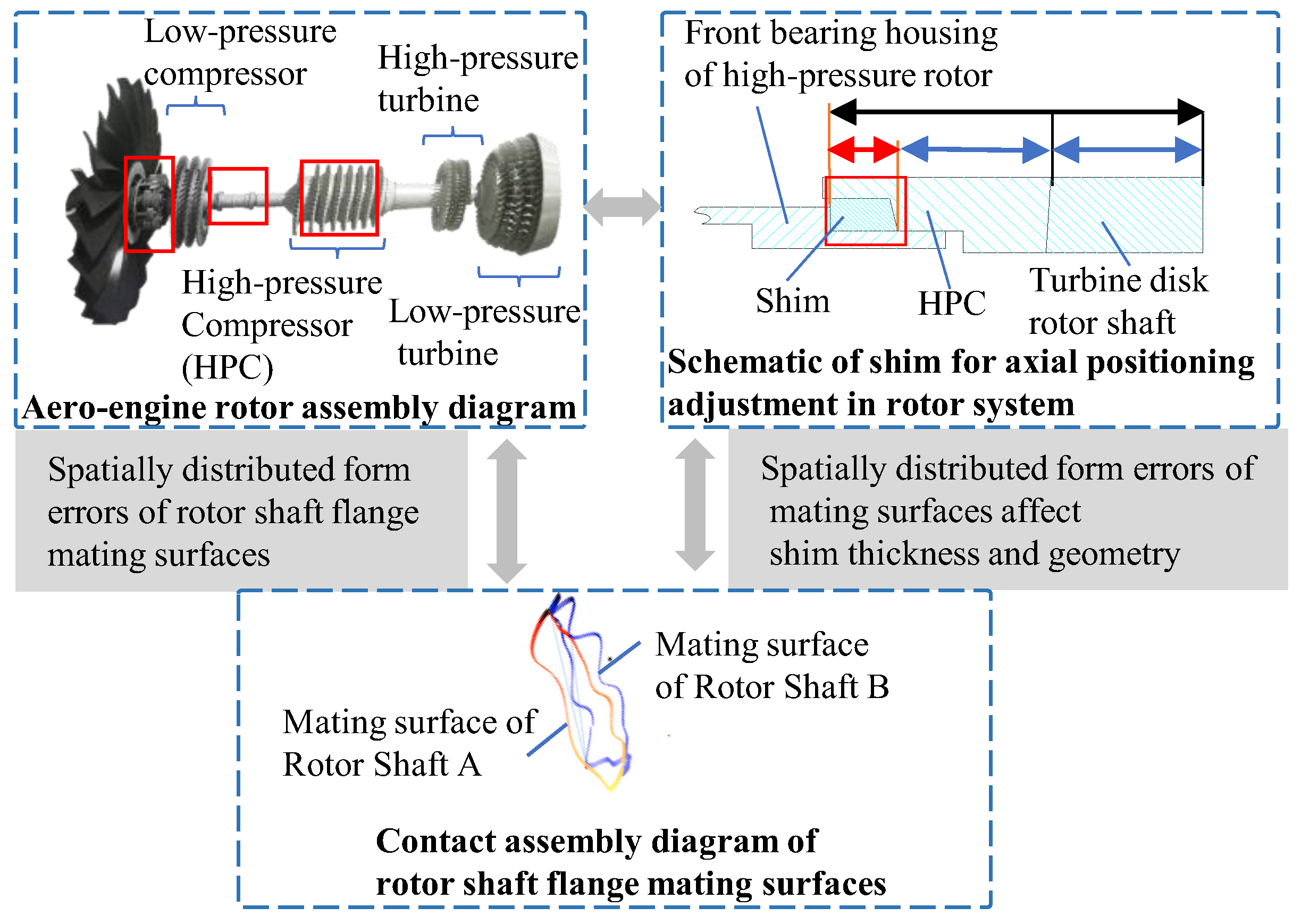
During the design phase, a dimensional chain analysis serves as a critical tool for the rational tolerance allocation of components [1], while providing essential references for subsequent control of the machining and assembly accuracy. With increasing product complexity and higher integration of component structures, the conventional dimensional chain analysis methods face significant challenges. In high-complexity and large-dimension scenarios, such as aero-engines, the effects of error propagation and accumulation substantially complicate dimensional chain analyses. This study focused on the influence of geometric errors, particularly the spatial distribution of form errors, on spatial dimensional chains. Spatially distributed form errors refer to the widely spaced deviations of the real surface from the nominal surface [2]. Such errors result in inconsistent clearances. As illustrated in Figure 1, the impact of spatially distributed form errors on the final assembly accuracy is demonstrated. The figure shows that when a plane with spatially distributed form errors is assembled with an ideal plane, the non-uniform distribution of form errors within the error area induces a rotational displacement of the ideal plane. Furthermore, as shown in Figure 2, the casing assembly consists of multiple components. The combined effects of dimensional errors in individual parts, geometric errors of mating surfaces, and multidirectional constraints on composite mating surfaces of the flange interfaces (including both axial constraints such as end-face contacts and radial constraints such as spigot fits) may lead to out-of-spec closed-loop dimensions (e.g., coaxiality errors in the casing assembly), potentially requiring assembly process adjustments that extend the production lead time and increase manufacturing costs. As shown in Figure 3, the axial assembly distance of the rotor is a critical parameter in ensuring aero-engine assembly quality. However, due to geometric errors at component mating surfaces, the axial relative positioning between the high-pressure compressor rotor and turbine rotor requires multiple trial assemblies to select appropriate shims for dimensional compensation. When treating either the shim thickness or post-assembly axial clearance as the closing loop, the accurate determination of this loop becomes key to reducing aero-engine manufacturing costs. The complexity of assembly analyses stems from multiple factors, including the large dimensions of component mating surfaces, cumulative errors during multicomponent assembly, and complex multiconstraint mating relationships at assembly interfaces. A conventional dimensional chain analysis is inadequate in addressing these challenges, creating an urgent need to develop distributed-form-error-based spatial dimensional chain analysis methods.

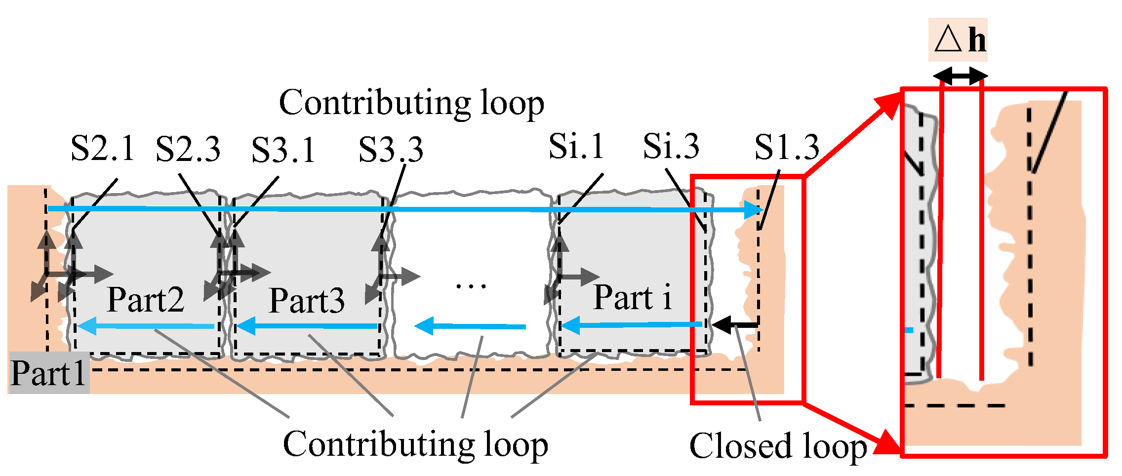
Previous studies have developed various types of dimensional chain models. For instance, one-dimensional or two-dimensional assembly dimensional chains were established based on 2D drawings, followed by traditional numerical analysis methods such as the worst-case method [3,4,5] and statistical method [6] to calculate assembly errors in the dimensional chain. Subsequently, manual tolerance allocation and optimization were performed based on engineering experience. However, these methods fail to fully account for (1) geometric errors of mating surfaces in 3D space, (2) coupling effects between assembly features, and (3) multidimensional characteristics of closed loops. Consequently, when applied to dimensional chains involving large-scale mating surfaces (which cannot be simplified as points) where geometric errors are non-negligible, they produce inaccurate tolerance design results. Several studies have developed three-dimensional spatial dimensional chain models, such as the tolerance map (T-MAP) model [7,8,9]. Chase et al. [10,11,12,13] employed two-dimensional and three-dimensional direct linearization methods, respectively, to convert deviations caused by geometric tolerances into dimensional deviations. Clément et al. applied the small displacement torsor (SDT) model [14,15,16,17,18,19,20], which utilizes deviation torsors and clearance torsors to describe geometric deviations and mating clearances between parts, and solves functional requirements through algebraic composition operations. Other researchers have approached dimensional chain modeling from the perspective of geometric relationship propagation. Desrochers and Rivière [21] proposed a matrix model, arguing that feature variations relative to a datum can be decomposed into six independent components—three translational displacements along the coordinate axes and three rotational displacements about the axes. Wang et al. [22] introduced a CAD-model-based automated generation method for 3D assembly dimensional chains using graph theory. El Mouden et al. [23] developed a 3D tolerance analysis method combining the Jacobian matrix with the torsor model, improving the computational efficiency for complex assemblies. Additionally, Zhang et al. [24] proposed a 3D tolerance zone computation method based on SDT, robotic kinematics, and convex set theory models, addressing challenges in process dimensioning and tolerance design for 3D manufacturing. Jain [25] proposed a method by fitting an orthotope inside an ellipsoid, employing the system Jacobian matrix to address challenges in tolerance analyses, tolerance allocation, and compensator selection. Tang et al. [26] introduced an improved Monte Carlo simulation approach utilizing surrogate models and low-discrepancy sequences, significantly enhancing the computational efficiency in dimensional variation analyses while maintaining accuracy. In another study [27], the authors developed a tolerance analysis tool based on Monte Carlo simulation to mitigate assembly rework caused by dimensional variability in prefabricated and offsite construction, subsequently reducing the rework risks through process optimization. Additionally, McGregor [28] applied a support vector regression (SVR) machine learning approach to develop a geometric shape prediction and qualification tool based on manufacturing parameters and feature descriptors, effectively predicting and diagnosing geometric defects in additive manufacturing while improving the part classification accuracy. Maltauro et al. [29] introduced the concept of variable-dependent admissible limits for tolerance stack-up analyses, where the limits are adaptively adjusted based on both geometrical and non-geometrical variables. While the aforementioned studies have made positive contributions to tolerance accumulation in geometric relationship transmission, these spatial dimension chain models face two primary limitations. First, most models are tolerance-based, where the tolerances merely describe the permissible variation range of geometric errors. Such approaches oversimplify the situation by reducing the geometric errors to ‘extreme boundaries’ within tolerance zones, treating post-machining surface form errors as scalar quantities (as shown in Figure 3). In reality, form errors exhibit spatial distributions. Second, in conventional dimension chains, the closed loop is typically represented by a scalar quantity (such as Δh in Figure 4) as the accumulation result. However, due to the stacking of spatially distributed form errors and other geometric errors, the closed-loop clearance actually demonstrates multidimensional spatial distribution characteristics, leading to discrepancies between design values and actual assembly outcomes. Under high-dimensional and large-scale conditions with limited part quantities, assembly process adjustments through part replacement become unfeasible. Consequently, accurate dimension chain prediction during the design phase can fundamentally reduce the subsequent manufacturing costs, time expenditures, and labor requirements. Moreover, precise dimension chain prediction at the design stage can provide optimized feedback for more accurate tolerance allocation. Thus, developing methods to obtain more precise dimension chain prediction results, thereby achieving more accurate tolerance allocation outcomes, represents an urgent and significant challenge.

Meanwhile, in practical engineering, geometric errors propagate through the geometric relationships in the dimensional chain. The constrained mating surfaces of parts often involve more than one pair of critical interfaces (as shown in Figure 4, where the key mating surface of part 2 serves as a key datum plane in the dimensional chain, with its position and orientation jointly constrained by both the horizontal plane and the left vertical plane of part 1). The resulting three-dimensional error coupling from these constraints ultimately directly affects the product performance. Zhang et al. [30,31] proposed a method for solving contact problems of mating surfaces by considering spatially distributed form errors. While these studies account for the influence of spatially distributed form errors on assembly posture, they primarily focus on single-reference assembly problems (i.e., assemblies constrained by only one pair of mating surfaces), with limited research on posture constraints imposed by dual mating surfaces. Liu et al. [32] introduced a general analysis method incorporating the parallel effects of geometric structures, utilizing constrained registration to compute the optimal mating results. Shi et al. [33] comprehensively considered the influence of the surface morphology and non-uniform contact deformation on the error propagation process, further adopting a phase optimization method to improve the assembly accuracy of multistage rotors. However, these methods primarily focus on error propagation mechanisms, while the systematic modeling of geometric constraints and assembly relationships within dimensional chains remains unresolved.

In response to the aforementioned challenges, the main contributions of this work are as follows: (1) We developed a distributed-form-error-driven spatial dimension chain model establishing mapping relationships between geometric features and functional dimensions through six-dimensional vector functions. The model incorporates spatially distributed form errors in datum definitions and employs the transfer matrix method to represent closed loops in both positional and orientational dimensions, enabling high-fidelity error prediction for large-scale assemblies. (2) We addressed multiple mating surface constraints by characterizing form errors and 3D coupled errors using 6-DoF geometric error components, significantly reducing the computational complexity while improving the prediction accuracy. (3) Non-mating-constrained datum errors were characterized using 6-DoF geometric error components based on spatially distributed form errors and modified envelope conditions, ensuring interchangeability and assembly quality. (4) We validated the model through a casing assembly case, demonstrating its effectiveness in analyzing six-dimensional closed-loop characteristics. (5) We applied the proposed six-dimensional spatial dimension chain model to the tolerance optimization design of aero-engine casing components, where its multidimensional error prediction capability facilitates precision tolerance allocation.

2. Six-Dimensional Spatial Dimension Chain Modeling

The proposed six-dimensional spatial dimension chain (SDC) model accounts for spatially distributed form errors during the design stage. The processing of the spatially distributed form errors follows the methodology in [34]—an error modeling approach that considers the distribution patterns of form errors induced by existing manufacturing processes at the design phase. This approach is predicated on the assumption that the machining errors remain statistically stable during a machine tool’s precision stability period. The machining errors on part surfaces comprise systematic errors and random errors. Systematic errors, as deterministic components, exhibit repeatability and predictability, constituting the dominant portion of the total errors; random errors lack regularity and typically account for a minor proportion. To establish manufacturing-process-referenced spatially distributed form errors, we inspect historically machined workpieces and employ NURBS (non-uniform rational B-spline)-based surface regression [35] to extract and separate systematic and random errors, subsequently utilizing the systematic error morphology (including both magnitude and spatial distribution patterns) as the primary error model component. Anwer et al. [36] made significant contributions to the field of tolerance analysis [37,38] by developing skin-model-based approaches, which utilize statistical distributions and idealized geometric deviation assumptions. In contrast to these methods, the present work establishes a fundamentally distinct manufacturing-feature-driven modeling process based on actual machining process data.

2.1. Definition of Modeling Data

The error modeling method based on existing manufacturing processes and the NURBS surface regression method for extracting systematic errors serve as the foundational error data for constructing the SDC model. The core of SDC modeling lies in establishing constraint relationships between geometric elements (e.g., planes, axes) and analyzing error accumulation through a datum reference system. In this study, the term ‘datum’ refers to a theoretically exact feature (as defined in ISO GPS [39]). Its closed-loop characteristic relies on well-defined geometric data and constraint propagation paths. Thus, defining a datum coordinate system via geometric elements (e.g., mating surfaces) to constrain the error directions constitutes the fundamental requirement for establishing an SDC. Subsequently, the modeling data for mating surfaces are selected and classified. Since most parts demand high assembly precision and exhibit substantial rigidity, deformation is not considered in this model. Therefore, this study operated under the assumption of rigid body conditions.

As shown in Figure 5, when considering the influence of spatially distributed form errors [31], the data are categorized based on the constraint properties of mating surfaces:

• Mating-constrained datum planes: The coordinate systems are established at both the ideal mating positions (e.g., surface b or c) and the actual mating positions (e.g., surface b′), referred to as the ideal mating-constrained datum and actual mating-constrained datum, respectively;
• Non-mating-constrained datum planes: The coordinate systems are defined at the ideal locations of critical surfaces (e.g., surfaces a and d) and their actual locations (e.g., surfaces a′ and d′), designated as the ideal non-mating-constrained datum and actual non-mating-constrained datum, respectively.

2.2. Establishment of SDC

Next, the SDC model with planar mating surfaces is constructed to characterize the mapping relationships between geometric features and functional dimensions.

The definition of the starting point in the SDC model affects its mathematical formulation. Since this section focuses on methodological research, the following fundamental rules are adopted to ensure the generality of the SDC model and to align with conventional measurement or design datum selection practices:

• The assembly datum plane of the component is selected as the primary reference for the global coordinate system of the SDC model;
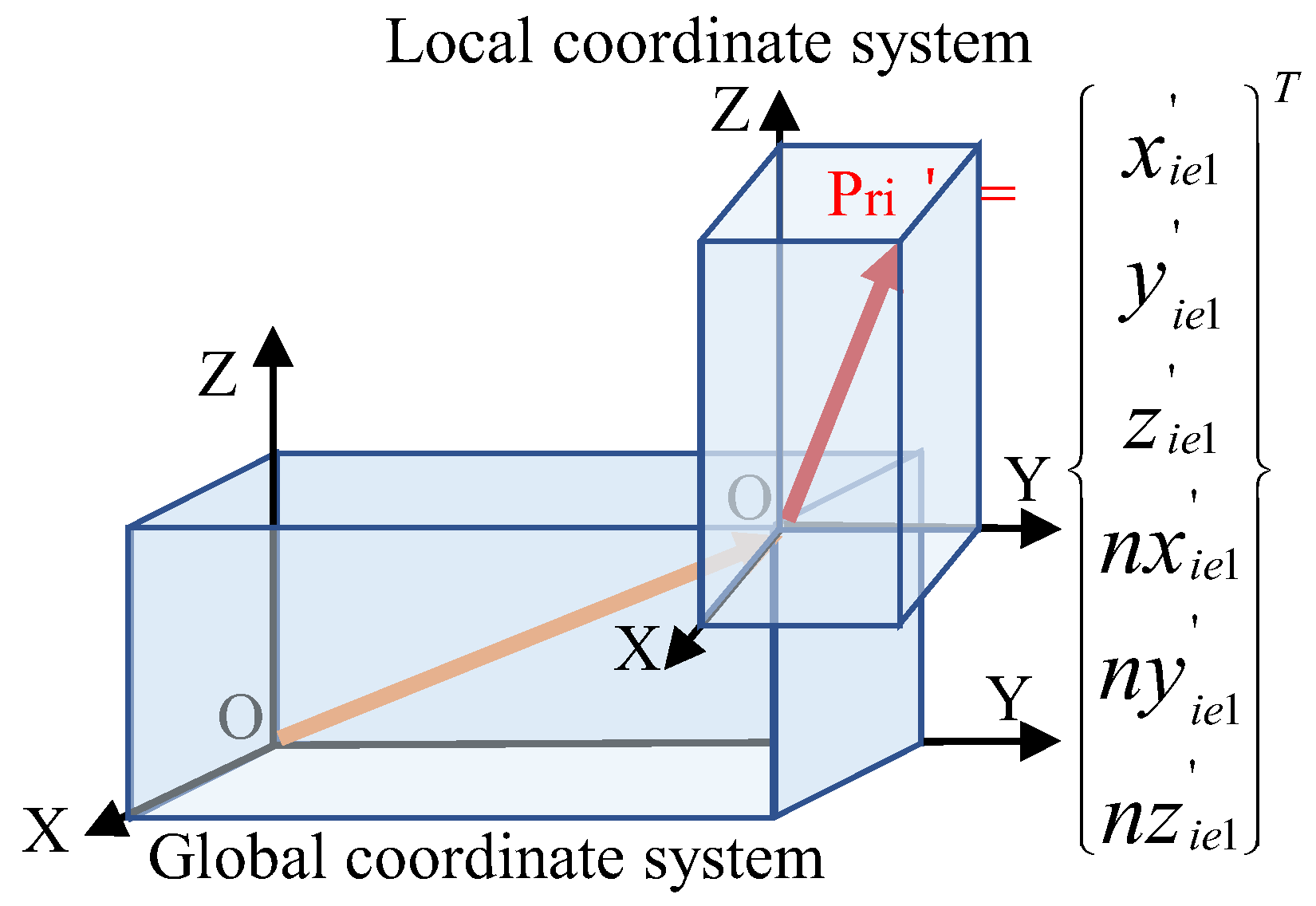
• Local coordinate systems are then established on the critical surfaces of the part, with their relationship to the global coordinate system illustrated in Figure 6;
• The SDC model is then decomposed into two branches:
  • First branch: Starting from the assembly datum (i.e., the origin of the global coordinate system), local coordinate systems are sequentially constructed along the transmission path of the contributing loops until reaching the datum plane at one end of the closed loop.
  • Second branch: Similarly, starting from the assembly datum, the process continues until reaching the datum plane at the other end of the closed loop.
  • Figure 7 illustrates the implementation of this principle via a distributed-form-error-based multidimensional SDC framework, covering both its construction and application (specific variables are detailed in the following two paragraphs).

The mechanistic implementation of this workflow is demonstrated through a representative case study, as shown in Figure 8. Based on the fundamental rules of modeling, mating surface S1.1 of part 1 serves as the assembly datum for the system. Therefore, the global coordinate system is established at the geometric center of mating surface S1.1/2.1. Subsequently, part 2 is assembled relative to part 1, and local coordinate systems are defined at their key mating surfaces—the ideal mating-constrained data (S1.1 and S2.1) and the actual mating-constrained datum (S1.1/2.1). The geometric error of the actual mating-constrained datum S1.1/2.1 from the ideal mating-constrained datum S2.1 is defined as the mating-constrained datum error M_2.1. (In this study, the mating-constrained datum error refers to the error between the ideal and actual mating-constrained data caused by spatially distributed form errors of critical surfaces.) This geometric error can be treated as a contributing loop with a nominal dimension of zero and incorporated into the contributing loops of part 2.

Similarly, when assembling part 3 relative to part 2, the local coordinate systems are defined at their key mating surfaces—the ideal mating-constrained data (S2.3 and S3.1) and the actual mating-constrained datum (S2.3/3.1). The geometric error M_2.3 between S2.3/3.1 and S2.3 is also treated as a zero-nominal-dimension contributing loop and merged into part 2’s contributing loops. The homogeneous transformation matrix (HTM) H_i characterizes the pose variation between ideal datum planes within the loop (e.g., H₂ represents the relationship between datum planes S2.1 and S2.3), where the translation matrix T_i describes positional offsets and the rotation matrix R_i accounts for angular changes in Equation (1). In Figure 8, elements connected by arrows of the same color belong to the same contributing loop. The set of contributing loops is denoted as {C_b1, C_b2, …, C_bi}.

$$H_i=\left[\begin{array}{cc}{R}_i& T_i\\ 0& 1\end{array}\right]$$

(1)

This assembly logic applies recursively to part i (where i denotes the generic part index). At the non-mating-constrained critical surfaces, the ideal non-mating-constrained datum (Si.3) and actual non-mating-constrained datum (Si.3’) are established. The error between them is defined as the non-mating-constrained datum error N_i.3. (Here, the non-mating-constrained datum error refers to the error between the ideal and actual non-mating-constrained data due to spatially distributed form errors.) The spatial vector gap between part i’s actual non-mating-constrained datum (Si.3’) and part 1’s actual non-mating-constrained datum (S1.3’) forms the closed loop (C_s).

The relationship between the geometric features (the mating-constrained datum error (M), the non-mating-constrained datum error (N), and SDC contributing loops) and the functional dimension (SDC closed loop C_s) is illustrated in Figure 8.

As demonstrated above, the integration of the error modeling method based on the current machining process with the NURBS surface regression method provides an effective solution for extracting, generating, and characterizing spatially distributed form errors. The transfer matrix method (TMM) employs rigid body kinematics to model pose errors (position + orientation) caused by geometric error propagation, and can also analyze coupled errors between geometric features (e.g., coupling errors caused by multimating surface constraints). However, it does not directly provide geometric error constraint relationships (e.g., assembly functional requirements). The conventional dimension chain models, based on tolerance boundaries or deviation analysis, disregard the influence of spatially distributed form errors. Consequently, they fail to characterize the non-uniform distribution of form errors in actual machining processes, inadequately describe 3D spatial error coupling, and lack precision in representing spatially distributed geometric features and critical functional dimensions. To address these limitations, this study integrates spatially distributed form errors, derived from the geometric error modeling method based on the current machining process and the NURBS surface regression method, with the transfer matrix into an SDC model. Furthermore, the SDC model is constructed using a six-dimensional vector function, establishing the mapping relationship between the geometric features and functional dimensions, as illustrated in Figure 9.

Here, P_ri′ (i = 1,2) denotes the pose of the closed-loop datum in the global coordinate system. The spatial gap of the closed loop is defined as the relationship between a pair of six-dimensional closed-loop datum coordinate systems P_ri′. Based on this relationship, additional multidimensional closed-loop parameters can be derived, such as the maximum and minimum distances of closed loops and the parallelism of one datum plane relative to another. In Figure 9, (x₁,y₁) and (x₂,y₂) represent the boundary ranges of the closed-loop data. The closed-loop datum plane P_ri′ is defined in the local coordinate system with the origin position vector [o_x, o_y, o_z, 1]^T and unit normal vector [n_ox, n_oy, n_oz, 0] ^T (e.g., [0, 0, 1, 0]^T for Z-normal planes, respectively. The mating-constrained and non-mating-constrained datum plane errors are formulated as small displacement screws M and N, respectively (Equation (2)). Each component of M and N represents an error along six degrees of freedom, including rotations about the x-, y-, and z-axes and translations along these axes (Figure 10).

$$M=\left(\Delta {\alpha }_i,\Delta {\beta }_i,\Delta {\gamma }_i,\Delta x_i,\Delta y_i,\Delta {\mathrm{z}}_i\right); N_{ie}=\left(\Delta {\alpha }_{ie},\Delta {\beta }_{ie},\Delta {\gamma }_{ie},\Delta x_{ie},\Delta y_{ie},\Delta {\mathrm{z}}_{ie}\right)$$

(2)

Next, the key parameters of the SDC model are characterized. The actual mating-constrained datum and its error (M) are derived in Section 2.3, while the non-mating-constrained datum and its error (N) are addressed in Section 2.4. Finally, an aero-engine casing assembly case study (Section 2.5) demonstrates the model’s application, with the validation results discussed in Section 3.

2.3. Characterization for Mating-Constrained Datum Error

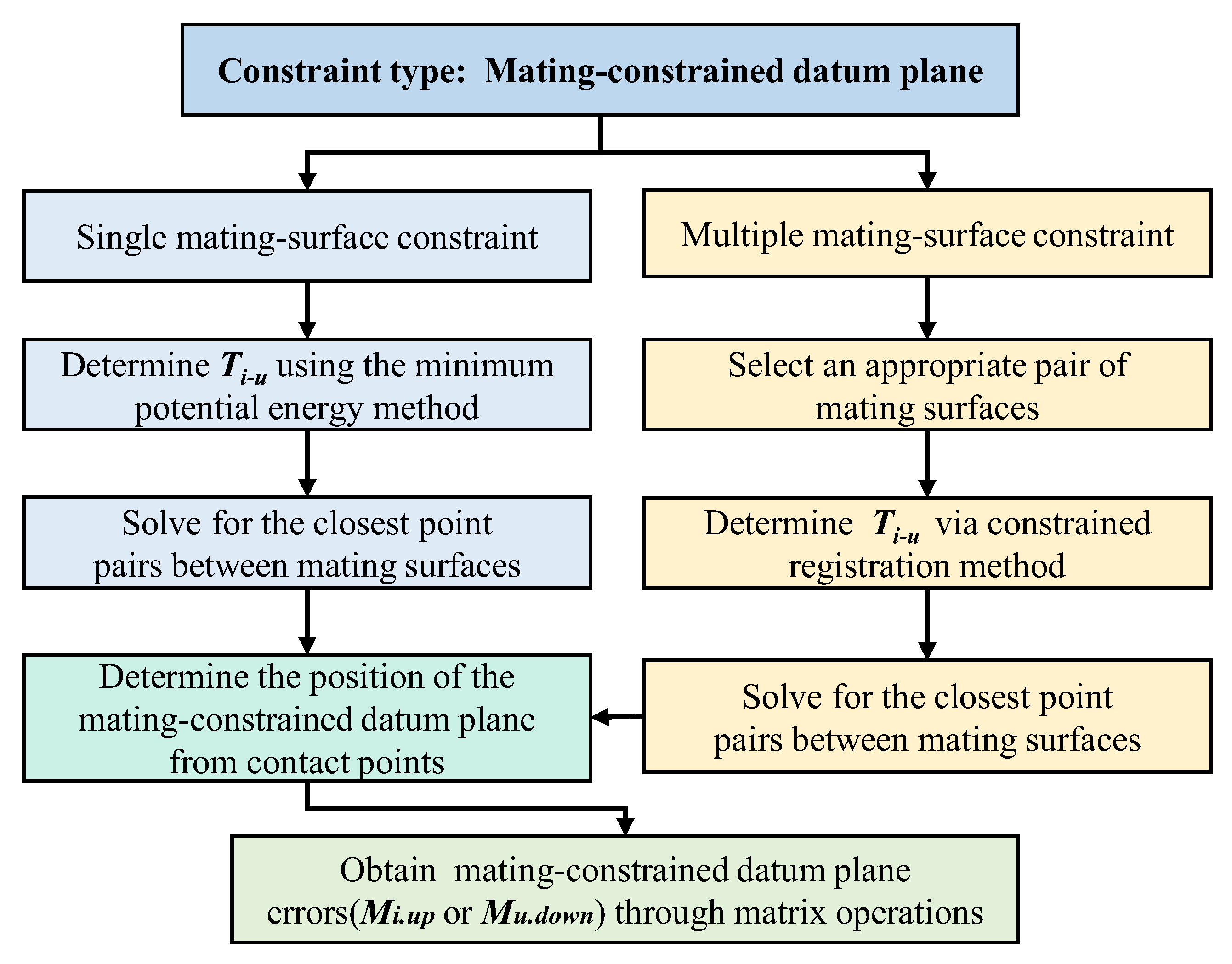
As illustrated in Figure 11, the middle panel serves as the primary schematic. A global coordinate system is established at the assembly datum, followed by the sequential assembly of part A and part B. The distance between the top surface of part B and the bottom surface of part A constitutes the closed loop, while the spatial distances between the top and bottom surfaces of part A and part B act as the contributing loops. The mating surfaces of both parts belong to the mating-constrained datum plane category. Based on the quantity of mating surfaces, the mating-constrained datum planes are classified into the single mating surface constraint (SMSC, left panel of Figure 11) and the multiple mating surface constraint (MMSC, right panel of Figure 11). The subsequent analyses focus on characterizing the mating-constrained datum plane and solving its associated errors under both scenarios, with the key procedural steps detailed in Figure 12.

(1) The SMSC: As shown in the left panel of Figure 11, the coordinate system of the mating-constrained datum plane is established at both the ideal mating position (critical surfaces T1’ and T2’) and the actual mating position (critical surfaces T1 or T2). The mating-constrained datum error, denoted as $M=\left(\Delta {\alpha }_i,\Delta {\beta }_i,\Delta {\gamma }_i,\Delta x_i,\Delta y_i,\Delta {\mathrm{z}}_i\right)$, corresponds to the error between the ideal mating-constrained datum plane T1’ and the actual mating-constrained datum plane T1, or between T2’ and T2. This error is characterized by six geometric error components, including rotations about and translations along the x-, y-, and z-axes.

The mating-constrained datum error is solved using the minimum potential energy method, with the following steps.

When the assembly reaches a stable state [30], the potential energy of part B relative to part A is minimized. The optimization objective is to minimize the potential energy of part B relative to part A, with the constraint that the mating surfaces of parts A and B do not interfere, as specified in Equation (3). The bare bones particle swarm optimization (BBPSO) algorithm is employed to determine the optimal solution for matrix T_i-u and to identify three pairs of contact points on the two mating surfaces (three non-collinear contact points ensure a stable assembly).

The surface containing these three contact points on the same part defines the actual mating-constrained datum plane (T1 or T2). Through matrix operations, the six-degree-of-freedom (6-DoF) geometric error components of the ideal mating-constrained datum plane T1’ relative to the actual mating-constrained datum plane T1 (denoted as $M_{u.down}$) and those of T2’ relative to T2 (denoted as $M_{i.up}$) can be obtained. The matrix relationship among T_i-u, $M_{i.up}$, and $M_{u.down}$ is then given by Equation (4).

$$\min {\displaystyle \sum (T_{i-u}\cdot {{\displaystyle D}}^1-{{\displaystyle D}}^2)}mg S.T. T_{i-u}\cdot {{\displaystyle D}}^1-{{\displaystyle D}}^2\ge 0$$

(3)

Here, D¹ and D² represent the point cloud data of the mating surfaces of part A and part B in the assembly coordinate system, respectively. The term (T_i-u·D¹ − D²) denotes the distance between part A and part B, where m is the mass of each point and g is the gravitational acceleration (a constant).

$$\begin{array}{l}{T}_{i-u}=E{R}_{i.up}\cdot E{R}_{u.down}\\ =\left[\begin{array}{cccc}1& -\Delta {\gamma }_{i.up}& \Delta {\beta }_{i.up}& \Delta x_{i.up}\\ \Delta {\gamma }_{i.up}& 1& -\Delta {\alpha }_{i.up}& \Delta y_{i.up}\\ -\Delta {\beta }_{i.up}& \Delta {\alpha }_{i.up}& 1& \Delta {\mathrm{z}}_{i.up}\\ 0& 0& 0& 1\end{array}\right]\left[\begin{array}{cccc}1& -\Delta {\gamma }_{u.down}& \Delta {\beta }_{u.down}& \Delta x_{u.down}\\ \Delta {\gamma }_{u.down}& 1& -\Delta {\alpha }_{u.down}& \Delta y_{u.down}\\ -\Delta {\beta }_{u.down}& \Delta {\alpha }_{u.down}& 1& \Delta {\mathrm{z}}_{u.down}\\ 0& 0& 0& 1\end{array}\right]\\ =\left[\begin{array}{cccc}1+(-\Delta {\gamma }_{i.up}).\Delta {\gamma }_{u.down}+(\Delta {\beta }_{i.up})(-\Delta {\beta }_{u.down})& (-\Delta {\gamma }_{u.down})+(-\Delta {\gamma }_{i.up})+\Delta {\beta }_{i.up}.\Delta {\alpha }_{u.down}& \Delta {\beta }_{u.down}+(-\Delta {\gamma }_{i.up})(-\Delta {\alpha }_{u.down})+\Delta {\beta }_{i.up}& \Delta x_{u.down}+(-\Delta {\gamma }_{i.up})\Delta y_{u.down}+\Delta {\beta }_{i.up}.\Delta {\mathrm{z}}_{u.down}+\Delta x_{i.up}\\ \Delta {\gamma }_{i.up}+\Delta {\gamma }_{u.down}+(-\Delta {\alpha }_{i.up})(-\Delta {\beta }_{u.down})& \Delta {\gamma }_{i.up}.(-\Delta {\gamma }_{u.down})+1+(-\Delta {\alpha }_{i.up}).(\Delta {\alpha }_{u.down})& \Delta {\gamma }_{i.up}.\Delta {\beta }_{u.down}+(-\Delta {\alpha }_{u.down})+(-\Delta {\alpha }_{i.up})& \Delta {\gamma }_{i.up}.\Delta x_{u.down}+\Delta y_{u.down}+(-\Delta {\alpha }_{i.up}).\Delta {\mathrm{z}}_{u.down}+\Delta {\mathrm{y}}_{i.up}\\ -\Delta {\beta }_{i.up}+\Delta {\alpha }_{i.up}.\Delta {\gamma }_{u.down}+(-\Delta {\beta }_{u.down})& (-\Delta {\beta }_{i.up})(-\Delta {\gamma }_{u.down})+\Delta {\alpha }_{i.up}+\Delta {\alpha }_{u.down}& (-\Delta {\beta }_{i.up}).\Delta {\beta }_{u.down}+\Delta {\alpha }_{i.up}.(-\Delta {\alpha }_{u.down})+1& (-\Delta {\beta }_{i.up}).\Delta x_{u.down}+\Delta {\alpha }_{i.up}.\Delta y_{u.down}+\Delta {\mathrm{z}}_{u.down}+\Delta z_{i.up}\\ 0& 0& 0& 1\end{array}\right]\end{array}$$

(4)

Here, T_i-u describes the pose error of the ideal mating-constrained datum plane of the u-th part relative to that of the i-th part, caused by mating surface errors; Δx, Δy, and Δz denote the infinitesimal translations along the x-, y-, and z-axes, respectively; Δα, Δβ, and Δγ represent the infinitesimal rotations about the x-, y-, and z-axes, respectively.

(2) The MMSC: The conventional dimension chain methods consider only a single pair of mating surfaces along a specified direction while neglecting others, with a primary focus on dimensional magnitudes and tolerances. These methods fail to account for the coupled effects of geometric errors from two pairs of mating surfaces in different directions on the SDC.

To address these limitations, we first selected an optimal pair of mating surfaces (the pair of mating surfaces that maximally constrains the part’s degrees of freedom) to obtain a datum plane as the actual mating-constrained datum plane in the SDC model (Figure 11, right panel), based on the assembly dimension chain direction. Subsequently, based on the selected mating-constrained datum plane, the constrained registration method [40] was employed to characterize the actual mating-constrained datum plane and solve its associated 6-DoF error M.

Whether for SMSC or MMSC, the mating-constrained datum plane error is inherently linked to the part’s manufacturing process. Under different processes, the magnitude and range of the geometric error components vary, typically following a probability distribution such as a normal distribution. These variations in geometric error components ultimately influence the characterization and distribution of the SDC error.

The mating-constrained datum plane error is solved using the constrained registration method, with the following procedure.

A constrained registration optimization model is constructed to obtain the optimal solution for matrix T_i-u between the ideal mating-constrained datum planes T2’ and T1’ in a multimating surface assembly structure. When the two parts are stably assembled, three pairs of the closest points (approaching infinitesimal proximity to zero) are selected on the designated mating surfaces c and b as contact points. These three contact point pairs can be recorded as C1(x_1i, y_1i, z_1i, 1) and C2(x_2i, y_2i, z_2i, 1) (i = 1, 2, 3). The surfaces containing these three contact points on each part defines the actual mating-constrained datum planes T1 or T2. Subsequently, through matrix operations, the mating-constrained datum plane errors $M_{i.up}$ and $M_{u.down}$ can be obtained. Here, $M_{i.up}$ represents the geometric error of the ideal mating-constrained datum plane T2’ relative to the actual mating-constrained datum plane T2, while $M_{u.down}$ represents T1’ versus T1. The matrix relationship among T_i-u, $M_{i.up}$, and $M_{u.down}$ is given by Equation (4).

This methodology, which incorporates geometric errors (particularly spatially distributed form errors) and employs constrained registration to solve both the actual mating-constrained datum planes in SDC and their associated error (M) under the MMSC, effectively reduces the topological complexity in assembled component surfaces. Consequently, it achieves computational simplification while enhancing both the efficiency and accuracy of SDC predictions.

2.4. Characterization for Non-Mating-Constrained Datum Error

To ensure part interchangeability and assembly quality, this subsection introduces an improved envelope condition (also referred to as the envelope requirement in some standards) and proposes new definitions of the envelope surface and envelope area. The envelope surface is then used to characterize the actual non-mating-constrained datum plane, from which the non-mating-constrained datum plane error $N_{ie}=\left(\Delta {\alpha }_{ie},\Delta {\beta }_{ie},\Delta {\gamma }_{ie},\Delta x_{ie},\Delta y_{ie},\Delta {\mathrm{z}}_{ie}\right)$ is derived. This error is characterized by six geometric error components, including rotations about and translations along the x-, y-, and z-axes. As illustrated in Figure 13, taking a simplified cylindrical casing as an example, a global coordinate system is established at the assembly datum O, followed by the sequential assembly of part A and part B. The distance between the top surface of part B and the bottom surface of part A forms the closed loop. As established in Section 2.1, the top surface of Part B is a non-mating-constrained datum plane. To characterize this plane using the envelope surface, the envelope surface must first be determined based on the envelope condition—a constraint ensuring that the non-mating-constrained datum plane error maintains dimensional and form compliance with assembly requirements under error conditions.

The improved envelope condition further specifies four criteria:

• Envelope condition definition: The envelope condition is an error analysis method. The envelope condition bounds all elements of the spatially distributed form errors within the envelope surface, controlling the surface’s position, orientation, and form to meet interchangeability and assembly quality requirements.
• Envelope surface definition: In a given direction, an ideal surface approximates the actual surface, with its position and form satisfying the envelope condition (criterion 1 above).
• Envelope area definition: The envelope surface and actual plane must intersect at ≥3 points, forming a triangular area termed the envelope area.
• Maximization requirement: The envelope area must be maximized to closely conform to the actual error surface.

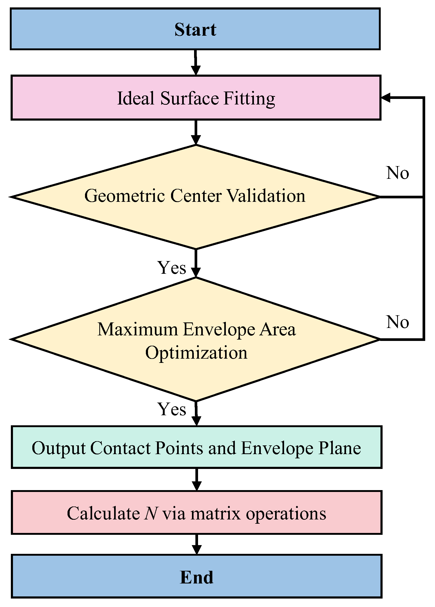
The envelope surface with the maximum envelope area is identified as the actual non-mating-constrained datum plane. Subsequently, the six-degree-of-freedom (6-DoF) non-mating-constrained datum plane error (N) of the envelope surface d′ relative to the ideal non-mating-constrained datum plane d is then derived. The characterization of the envelope surface and the solution for N are detailed below in Figure 14.

• Ideal Surface Fitting

An ideal datum plane is fitted to the actual error surface S through asymptotic convergence, subject to the following constraints. The ideal plane does not interfere with the actual error surface S, and there exist at least three contact points between the ideal plane and S, P₁(x₁′, y₁′, z₁′), P₂(x₂′, y₂′, z₂′), and P₃(x₃′, y₃′, z₃′), as formalized in Equation (5):

$$V\cdot \left(x_j,y_j,z_j\right)\le {}^0 \forall \left(x_j,y_j,z_j\right)\in S$$

(5)

where V is the normal vector of the envelope plane and (x_j, y_j, z_j) represents all measured points on S.

2.

Geometric Center Validation

Since the casing part is a hollow cylinder, its centroid must lie within the cavity. To ensure the envelope surface better conforms to the actual condition, the geometric center of the casing’s critical surface must lie within the triangle formed by contact points P₁, P₂, and P₃. If this condition fails, the algorithm returns to step 1.

3.

Maximum Envelope Area Optimization

To ensure the envelope surface maximally encompasses the actual surface for optimal conformity and improved model accuracy, the maximum envelope area (max S_area) must be determined. The envelope area S_area, defined by the contact points P₁, P₂, and P₃ (Equation (6)), is evaluated. If the condition is satisfied, the procedure proceeds; otherwise, it returns to step 1.

$$S_{area}={\displaystyle \frac{1}{2}}\times ‖({\displaystyle P2}-{\displaystyle P1})\times ({\displaystyle P3}-{\displaystyle P1})‖$$

(6)

where × denotes the cross product and $‖\cdot ‖$ the vector norm

4.

Output Contact Points and Envelope Plane

The coordinates of P₁, P₂, and P₃ are recorded, and the position of the envelope plane d′ is determined.

5.

Non-Mating-Constrained Datum Error Calculation

The 6-DoF geometric error components of d′ relative to the ideal datum plane d (denoted as N) are computed and output.

This subsection accounts for spatially distributed form errors and characterizes the actual non-mating-constrained datum planes error using more precise 6-DoF parameters. The N is correlated with the part’s manufacturing processes, as different processes yield varying error magnitudes and ranges that typically following probability distributions such as normal distributions. Variations in error ultimately affect the spatial distribution of the closed loop.

2.5. Six-Dimensional Modeling for Aero-Engine Casing Assembly

Taking the assembly of a simulated aero-engine casing as an example, we analyzed two typical assembly issues caused by geometric error accumulation: (1) an end-face closed-loop SDC, where the spatial distance of the closed loop is referenced to the flange end face as the datum plane; (2) an axis-based closed-loop SDC, where the coaxiality spatial error is referenced to the casing housing axis as the datum axis. Additionally,

Table 1. Comparative advantages of the SDC model for aero-engine casing assembly.

Key Issue	Limitation of Conventional Methods	SDC-Based Solution	Application Value
Flange spatially distributed form errors	Tolerance-based dimension chain modeling	SDC model incorporating spatially distributed form errors	Solves high-precision prediction of mating surfaces
Multiconstrained flange structure	Single mating surface constraint assumption (end face only)	Multimating surface constraints for 3D coupled errors	Enables 3D coupled error analyses in SDCs
Functional dimension representation	Scalar-based expression	Six-dimension parameters (position + orientation vectors)	Supports multidimensional spatial characterization

summarizes the advantages of the SDC model.

(1) SDC propagation law with the end face as the closed-loop datum.

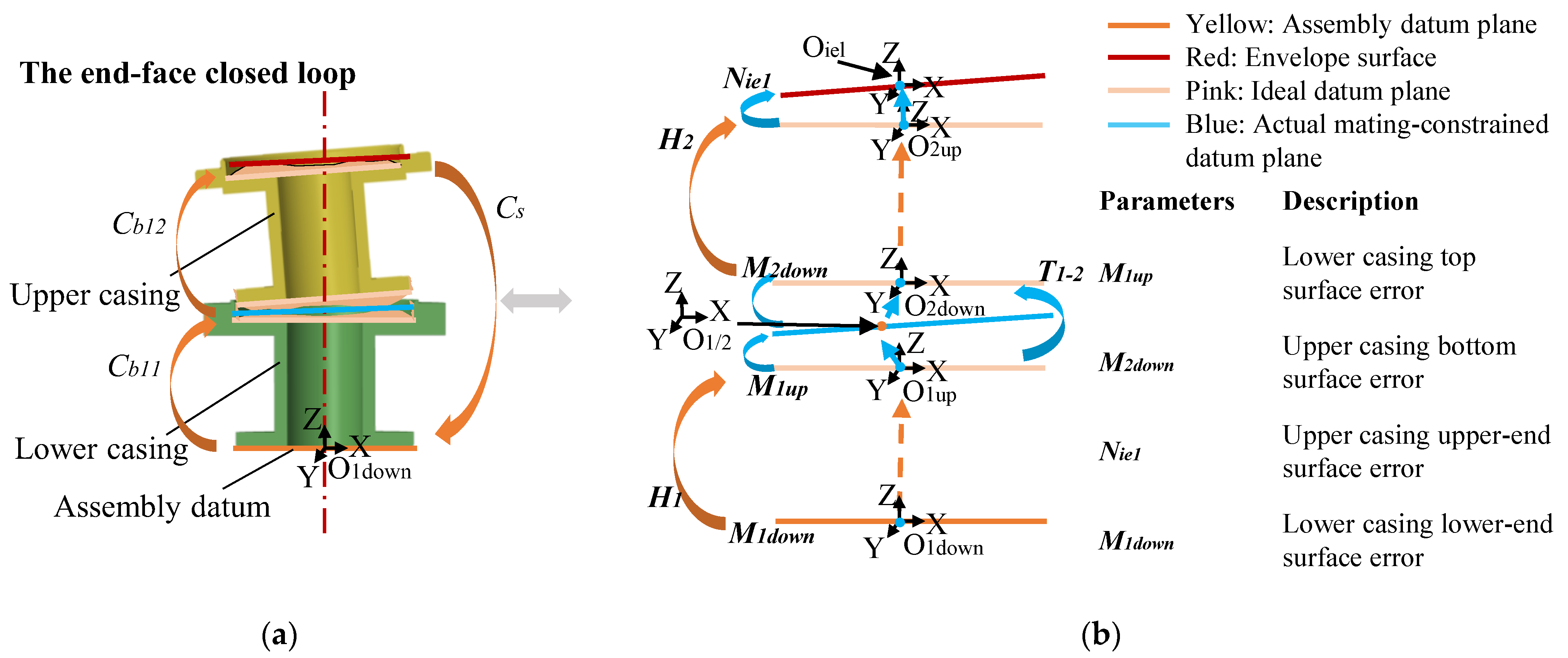
The contributing loops are C_b11 and C_b12, as shown in Figure 15a, with the closed loop C_s representing the spatial dimension from the upper end face O_iel of the upper casing to the assembly datum face O_ldown. Following the aforementioned computational process, the coordinate systems for critical surfaces are established and the influencing factors of SDC errors are analyzed, as depicted in Figure 15b.

The predominant error sources in SDC are:

• The mating-constrained datum plane error _M1up of the lower casing top surface O_lup (comprising two constrained surfaces—the flange end face and flange spigot cylindrical face);
• The mating-constrained datum plane error M_2down of the upper casing bottom surface O_2down (also including two constrained surfaces—the flange end face and flange spigot cylindrical face);
• The non-mating-constrained datum plane error N_ie1 at the end face of the upper casing’s top surface;
• The mating-constrained datum plane error _M1down at the end face of the lower casing’s bottom surface.

Here, the lower casing bottom end face and the assembly datum plane O_ldown are considered nominally ideal surfaces; therefore, the error component M_ldown can be disregarded.

The initial pose of the closed-loop datum plane P_r1’ is defined by the position vector of the coordinate system origin: O = [o_x, o_y, o_z, 1]^T; the unit normal vector of the datum plane: n = [n_ox, n_oy, n_oz, 0]^T (e.g., [0, 0, 1, 0]^T for Z-axis alignment).

The influence of geometric errors on the closed loop is analyzed using the transfer matrix method, where the pose of the closed-loop datum in the global coordinate system is characterized by a six-dimensional parameter P_r1’, as expressed in Equations (7) and (8). Finally, the closed-loop metrics are evaluated against assembly or design requirements. If the results are unsatisfactory, the process iterates for redesign optimization.

$$\begin{array}{c}{O}_{ie1}={({x_{ie1}}^{\prime },{y_{ie1}}^{\prime },{z_{ie1}}^{\prime },1)}^T\\ =H_1\cdot M_{1up}\cdot M_{2down}\cdot H_2\cdot N_{ie1}\cdot {\left[o_x,o_y,o_z,1\right]}^T\\ =H_1\cdot T_{1-2}\cdot H_2\cdot N_{ie1}\cdot {\left[o_x,o_y,o_z,1\right]}^T\\ =\left[\begin{array}{cccc}\cos {\beta }_1\cos {\gamma }_1& -\cos {\beta }_1\sin {\gamma }_1& \sin {\beta }_1& {\mathrm{x}}_1\\ \cos {\beta }_1\sin {\gamma }_1+\sin {\alpha }_1\sin {\beta }_1\cos {\gamma }_1& \cos {\alpha }_1\cos {\gamma }_1-\sin {\alpha }_1\sin {\beta }_1\sin {\gamma }_1& -\sin {\alpha }_1\cos {\beta }_1& y_1\\ \sin {\beta }_1\sin {\gamma }_1-\cos {\alpha }_1\sin {\beta }_1\cos {\gamma }_1& \cos {\alpha }_1\cos {\gamma }_1+\cos {\alpha }_1\sin {\beta }_1\sin {\gamma }_1& \cos {\alpha }_1\cos {\beta }_1& z_1\\ 0& 0& 0& 1\end{array}\right]\cdot \left[\begin{array}{cccc}1& -\Delta {\gamma }_{1-2}& \Delta {\beta }_{1-2}& \Delta x_{1-2}\\ \Delta {\gamma }_{1-2}& 1& -\Delta {\alpha }_{1-2}& \Delta y_{1-2}\\ -\Delta {\beta }_{1-2}& \Delta {\alpha }_{1-2}& 1& \Delta {\mathrm{z}}_{1-2}\\ 0& 0& 0& 1\end{array}\right]\\ \cdot \cdot \cdot \left[\begin{array}{cccc}1& -\Delta {\gamma }_{ie1}& \Delta {\beta }_{ie1}& \Delta x_{ie1}\\ \Delta {\gamma }_{ie1}& 1& -\Delta {\alpha }_{ie1}& \Delta y_{ie1}\\ -\Delta {\beta }_{ie1}& \Delta {\alpha }_{ie1}& 1& \Delta {\mathrm{z}}_{ie1}\\ 0& 0& 0& 1\end{array}\right]\cdot \left[\begin{array}{c}{o}_x\\ o_y\\ o_z\\ 1\end{array}\right]\end{array}$$

(7)

$$\begin{array}{c}{n}_{ie1}={(n{x}_{ie1}{}^{\prime },n{y}_{ie1}{}^{\prime },n{z}_{ie1}{}^{\prime },0)}^T=H_1\cdot M_{1up}\cdot M_{2down}\cdot H_2\cdot N_{ie1}\cdot {\left[n_{0\mathrm{x}},n_{0\mathrm{y}},n_{0\mathrm{z}},0\right]}^T=H_1\cdot T_{1-2}\cdot H_2\cdot N_{ie1}\cdot {\left[n_{0\mathrm{x}},n_{0\mathrm{y}},n_{0\mathrm{z}},0\right]}^T\end{array}$$

(8)

Here, M_1up, M_2down, and T_1–2 share the same definitions as discussed in Section 2.3. Similarly, N_ie1 retains the meaning introduced in Section 2.4:

$$H_i=H_{kj}=\left[\begin{array}{cccc}\cos {\beta }_{kj}\cos {\gamma }_{kj}& -\cos {\beta }_{kj}\sin {\gamma }_{kj}& \sin {\beta }_{kj}& \mathrm{x}\\ \cos {\beta }_{kj}\sin {\gamma }_{kj}+\sin {\alpha }_{kj}\sin {\beta }_{kj}\cos {\gamma }_{kj}& \cos {\alpha }_{kj}\cos {\gamma }_{kj}-\sin {\alpha }_{kj}\sin {\beta }_{kj}\sin {\gamma }_{kj}& -\sin {\alpha }_{kj}\cos {\beta }_{kj}& y\\ \sin {\beta }_{kj}\sin {\gamma }_{kj}-\cos {\alpha }_{kj}\sin {\beta }_{kj}\cos {\gamma }_{kj}& \cos {\alpha }_{kj}\cos {\gamma }_{kj}+\cos {\alpha }_{kj}\sin {\beta }_{kj}\sin {\gamma }_{kj}& \cos {\alpha }_{kj}\cos {\beta }_{kj}& z\\ 0& 0& 0& 1\end{array}\right]$$

(9)

where H_{i =} H_kj denotes the matrix representation of positional and orientational variations between multiple ideal datum planes on the same component within an SDC (e.g., the pose relationship between ideal datum planes O_2down and O_2up on the upper casing in Figure 15). It specifically describes the coordinate system pose relationship between the k-th and j-th critical surfaces on the i-th component. In the matrix, x, y, and z represent the displacements of coordinate system O_ij relative to O_ik along the x-, y-, and z-axes, respectively; α_kj, β_kj, and γ_kj denote the rotation angles of O_ij relative to O_ik about the x-, y-, and z-axes. In this case, i = 1, 2 …, k = 1 (constant), and j = 2 (constant).

From Equations (9) and (10), the position and orientation vector expression P_r1′ = {x_ie1′, y_ie1′, z_ie1′, nx_ie1′, ny_ie1′, nz_ie1′} is derived for datum plane O_2up at one end of the closed loop in the global coordinate system. Similarly, the position and orientation vector expression P_r2′ = {x_ie2′, y_ie2′, z_ie2′, nx_ie2′, ny_ie2′, nz_ie2′} is obtained for the other datum plane O_1down in the closed loop. In this example, to simplify the model description and avoid redundant terms, O_1down is treated as an ideal plane; hence, P_r2′ = {0, 0, 0, 0, 0, 1}. Consequently, the closed-loop characterization is given by Equation (12).

$$C_{sl}\left(close loop\right)=\left\{\begin{array}{c}{P}_{r1}{}^{\prime }=\{x_{ie1}{}^{\prime },y_{ie1}{}^{\prime },z_{ie1}{}^{\prime },n{x}_{ie1}{}^{\prime },n{y}_{ie1}{}^{\prime },n{z}_{ie1}{}^{\prime }\},x_1\in [x_{1c}-r,x_{1c}+r],y_1\in [y_{1c}-\sqrt{(r^2-{(x_1-x_{1c})}^2)}]\\ P_{r2}{}^{\prime }=\{x_{ie2}{}^{\prime },y_{ie2}{}^{\prime },z_{ie2}{}^{\prime },n{x}_{ie2}{}^{\prime },n{y}_{ie2}{}^{\prime },n{z}_{ie2}{}^{\prime }\}=\{0\},x_2\in [x_{2c}-r,x_{2c}+r],y_2\in [y_{2c}-\sqrt{(r^2-{(x_2-x_{2c})}^2)}]\end{array}\right.$$

(10)

Here, (x_1c,y_1c) and (x_2c,y_2c) represent the coordinates of the center points of the closed-loop end faces along the x- and y-axes, respectively, and r denotes the radius of the circle.

Based on Equation (10), the spatial six-dimensional distribution (position and orientation vectors) of a pair of datum planes for the end-face closed loop in the global coordinate system can be obtained. This further enables the derivation of parameters related to the end-face closed loop, such as the maximum and minimum spatial distances, parallelism, or relative normal vector relationship between the evaluated datum plane P_r1′ and the other datum plane.

(2) SDC propagation law with the axis as the closed-loop datum.

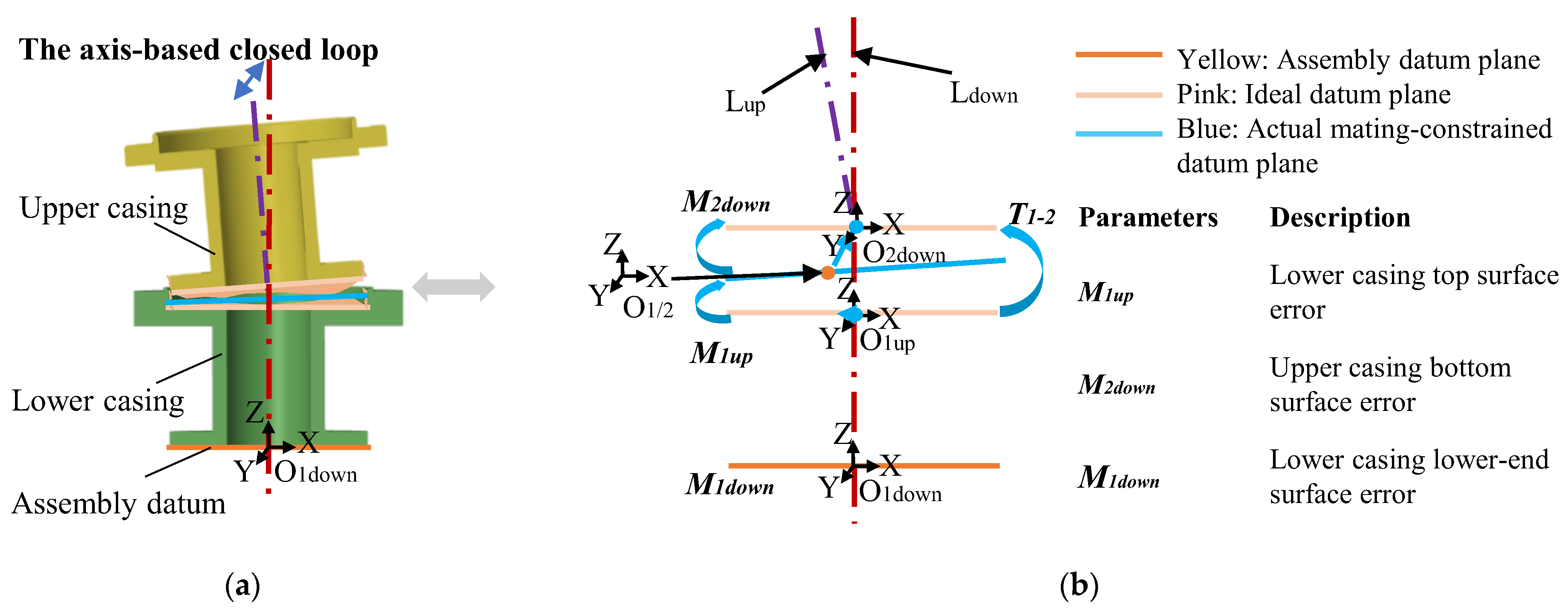
Based on the aforementioned computational process, the coordinate systems of critical surfaces are established (Figure 16). The primary error contributors in the SDC are:

• The mating-constrained datum plane error M_1up of the lower casing’s top surface (including two constraint surfaces—the flange end face and the flange spigot cylindrical surface);
• The mating-constrained datum plane error M_2down of the upper casing’s bottom surface (similarly comprising the flange end face and spigot cylindrical surface).

This model primarily analyzes spatially distributed form errors, while radial errors (e.g., cylindricity of the casing’s inner surface) and spatial relative positions (e.g., axial misalignment between upper and lower casings) remain uncharacterized.

For the closed loop, one datum axis L_down is defined by the equation L_down = {lx_ie′, ly_ie′, lz_ie′, nlx_ie′, nly_ie′, nlz_ie′}, where L_down (the assembly datum axis) is treated as a known value.

The initial pose of the other datum axis L_up is specified as:

• Position vector of the coordinate origin: [o_lx, o_ly, o_lz, 1]^T;
• Unit normal vector of the datum axis: [nl_ox, nl_ox, nl_ox, 0]^T (e.g., [0, 0, 1, 0]^T for Z-axis alignment).

After error propagation through the SDC, the pose of the closed-loop datum in the global coordinate system is described using a six-dimensional parameter L_up (position vector + orientation vector), as defined in Equations (11) and (12).

$$L_{ie1}={(l{x}_{ie1}{}^{\prime },l{y}_{ie1}{}^{\prime },l{z}_{ie1}{}^{\prime },1)}^T=H_1\cdot M_{1up}\cdot M_{2down}\cdot {\left[o_{lx},o_{ly},o_{lz},1\right]}^T=H_1\cdot T_{1-2}\cdot {\left[o_{lx},o_{ly},o_{lz},1\right]}^T$$

(11)

$$n{L}_{ie1}={(nl{x}_{ie1}{}^{\prime },nl{y}_{ie1}{}^{\prime },nl{z}_{ie1}{}^{\prime },0)}^T=H_1\cdot M_{1up}\cdot M_{2down}\cdot {\left[n{l}_{0\mathrm{x}},n{l}_{0\mathrm{y}},n{l}_{0\mathrm{z}},0\right]}^T=H_1\cdot T_{1-2}\cdot {\left[n{l}_{0\mathrm{x}},n{l}_{0\mathrm{y}},n{l}_{0\mathrm{z}},0\right]}^T$$

(12)

Here, M_1up, M_2down, H₁, and T_1–2 share the same definitions as in Equations (7) and (8).

Theorem-type environments (including propositions, lemmas, corollaries, etc.) can be formatted as follows. Consequently, the closed-loop expression (Equation (13)) is derived from Equations (11) and (12).

$$C_{sl}\left(close loop\right)=\left\{\begin{array}{c}{L}_{up}=\{l{x}_{ie1}{}^{\prime },l{y}_{ie1}{}^{\prime },l{z}_{ie1}{}^{\prime },nl{x}_{ie1}{}^{\prime },nl{y}_{ie1}{}^{\prime },nl{z}_{ie1}{}^{\prime }\},{{\displaystyle x}}_1\in [{{\displaystyle x}}_{1\min },{{\displaystyle x}}_{1\max }],{{\displaystyle y}}_1\in [{{\displaystyle y}}_{1\min },{{\displaystyle y}}_{1\max }]\\ L_{down}=\{l{x}_{ie}{}^{\prime },l{y}_{ie}{}^{\prime },l{z}_{ie}{}^{\prime },nl{x}_{ie}{}^{\prime },nl{y}_{ie}{}^{\prime },nl{z}_{ie}{}^{\prime }\}=\{0,0,0,0,0,1,0\},{{\displaystyle x}}_2\in [{{\displaystyle x}}_{2\min },{{\displaystyle x}}_{2\max }],{{\displaystyle y}}_2\in [{{\displaystyle y}}_{2\min },{{\displaystyle y}}_{2\max }]\end{array}\right.$$

(13)

Here, (x₁, y₁) and (x₂, y₂) represent the interval range of the datum axis for the closed loop. Based on Equation (13), the spatial six-dimensional distribution (position and orientation vectors) of the datum axis pair for the closed loop in the global coordinate system can be obtained. This further enables the derivation of coaxiality-related parameters, such as the spatial pose normal vector of the evaluated axis L_up and the coaxiality error itself.

3. Experimental Validation of the SDC Model for Casing Assembly

3.1. Experimental Design

The SDC model in this study is an error modeling method based on existing manufacturing processes, using the error distribution patterns induced by current machining techniques as design references. Machined casings from previous productions were inspected, and the corresponding systematic errors were extracted and separated using a NURBS-based surface regression method to serve as the primary errors in the SDC model. The validity of the SDC model was verified through casing assembly experiments.

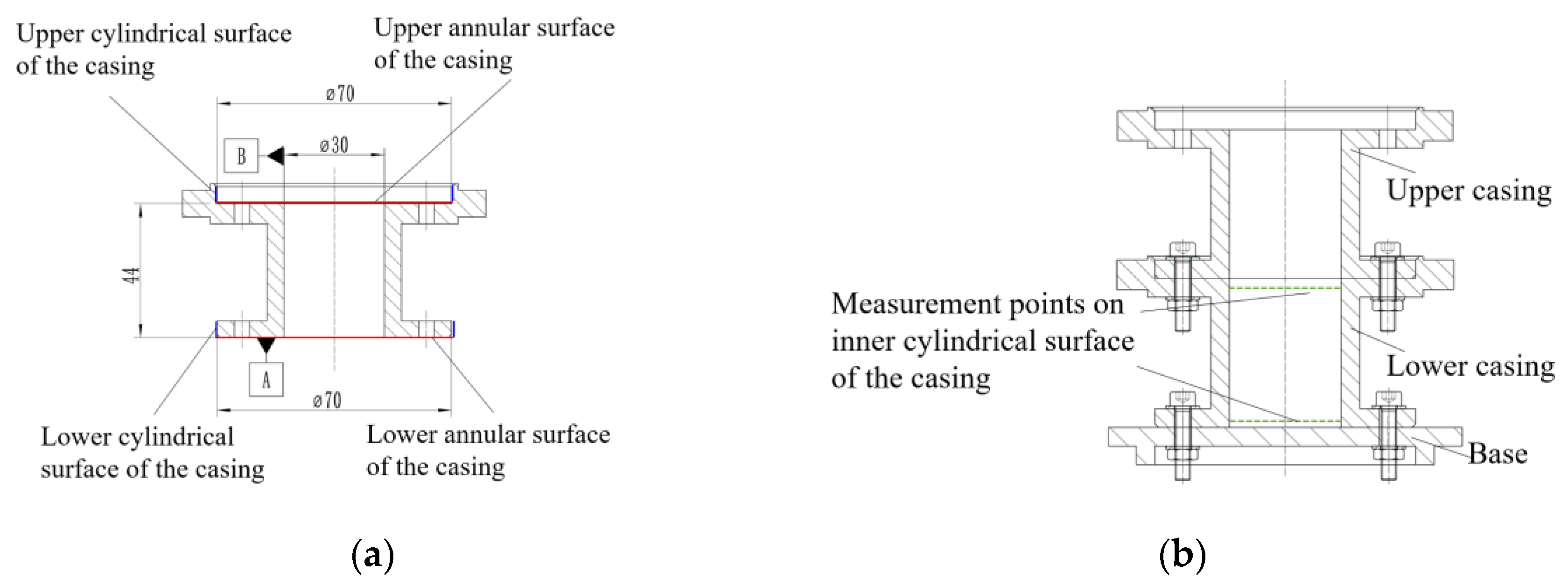
To enable multiple tests with a limited number of parts, several bolt holes were arranged on the flange end face, allowing the flange to be rotated at specific angles to obtain multiple sets of assembly results. The casing part samples are shown in Figure 17a, and the assembled casing structure is illustrated in Figure 17b. The upper surface of the base was ground to serve as an ideal assembly reference plane. To more clearly validate the multidimensional characteristics of the closed loop, the design tolerance band for the components was intentionally widened.

Using datum A, the parallelism of the upper annular surface of the lower casing was 0.121 mm, while that of the upper casing was 0.07 mm. The perpendicularity of the upper annular surface of the lower casing, relative to datum B, was 0.08 mm. Two upper casings (casing 1 and casing 2) and one lower casing were machined. During assembly, the cylindrical mating surfaces at the flange interface were designed as transition fits.

3.2. Experimental Procedure

3.2.1. Component Measurement

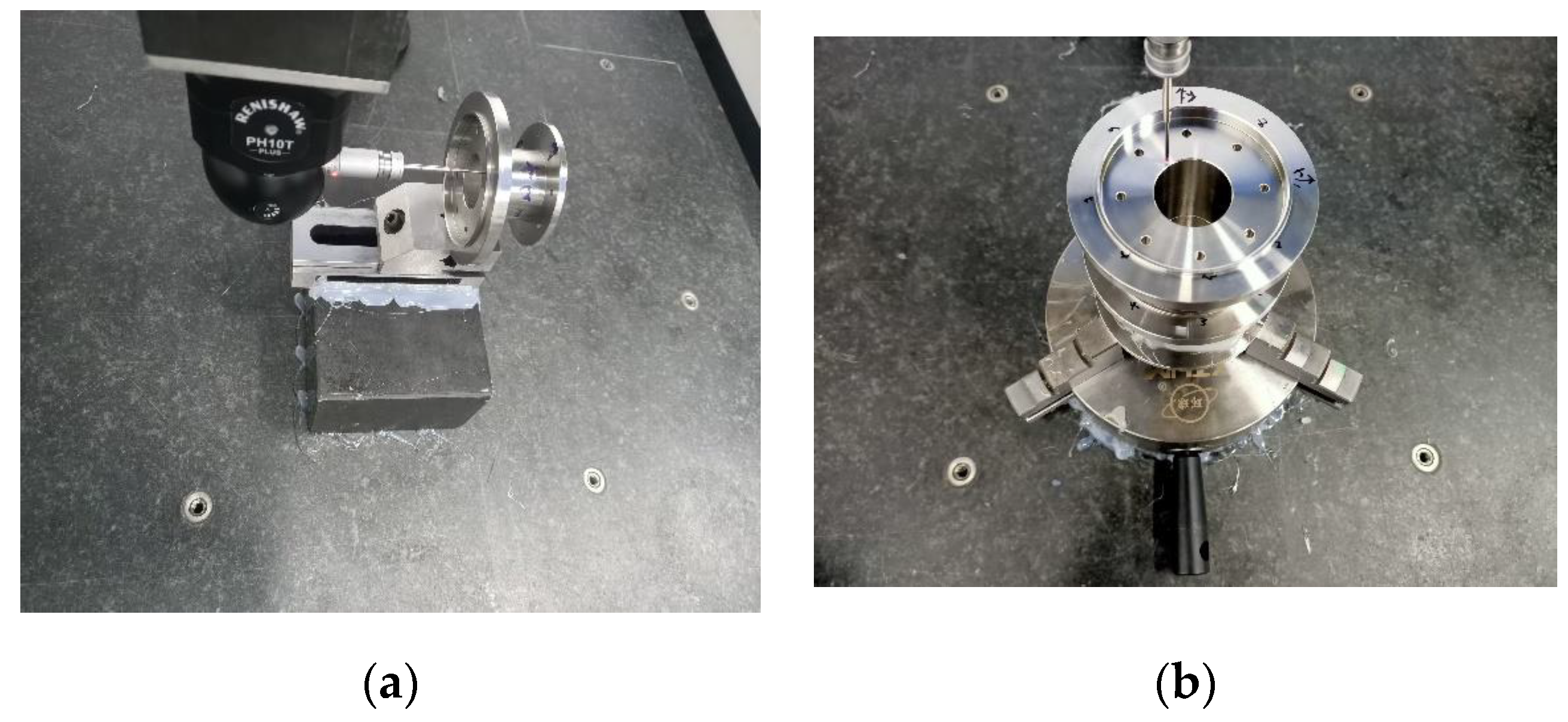
This study employed a coordinate measuring machine (CMM) to collect data points from the critical surfaces of the parts. The CMM model used was a Hexagon SCIROCCO 09.10.07, with a measurement uncertainty of (2.0 + 3L/1000) μm, and the software system was PC-DMIS 2020. The measured critical surfaces included the lower annular surface, lower cylindrical surface, upper annular surface, upper cylindrical surface, and inner cylindrical surface of the casing, as shown in Figure 17a. A total of 240 points were collected from five circular paths on both the upper and lower annular surfaces of the casing. For the cylindrical surfaces at the upper end of the lower casing and the lower end of the upper casing, 96 points were collected from two circular paths each (the number of points depended on the sampling interval, which was set to 3–5 mm in this study). The inner cylindrical surface of the casing was measured along two circular paths, totaling 16 points (the line connecting the centers of these circles was used as the part axis). All measurements were performed after CMM calibration, with the errors primarily being dependent on the equipment’s inherent accuracy. The orientation of the measurement coordinate system is illustrated in Figure 15. Taking the lower annular surface as an example, the coordinate system origin is located at the center of the lower annular surface, with the positive X-axis pointing to the right and the positive Z-axis pointing upward. The measurement of an individual part is shown in Figure 18a. To ensure experimental repeatability, two sets of experiments were conducted using casing 1 and casing 2 for the upper casing.

3.2.2. Assembly Measurement

(1) One objective of assembly measurement is to obtain the measured pose of the upper end face of the upper casing in the end face closed-loop model, as shown in Figure 18b. This allows the characterization of key parameters such as the envelope surface (one of the closed-loop datum planes), the distance from the envelope surface to the assembly datum (another closed-loop datum plane), the perpendicularity of the envelope surface relative to the lower casing axis, and its parallelism relative to the assembly datum plane—thereby validating the multidimensional characteristics and accuracy of the closed loop. (2) To further validate the model’s effectiveness, the second objective is to acquire spatial closed-loop parameters formed by the axes of the upper and lower casings in the axis-based closed-loop model, thereby deriving optimization-relevant metrics such as the coaxiality error.

As illustrated in Figure 15, an assembly coordinate system was established on the base, coinciding with the coordinate system of the lower casing’s bottom annular face. The lower casing served as the assembly datum, to which casing 1 was mounted and adjusted to a stabilized configuration before being secured with M3 bolts. Post-assembly, measurements were taken at the upper casing’s top annular face (240 points across 5 concentric circles) and the inner cylindrical surfaces of both upper and lower casings (16 points per cylinder, sampled in 2 separate circles), as shown in Figure 17b.

To ensure experimental repeatability and validate the impact of assembly phase differences between the upper and lower casings on the SDC model predictions—particularly when the same set of components exhibits identical spatially distributed form errors and geometric errors—the following procedure was implemented. Casing 1 was rotated clockwise around the z-axis by random angles to vary the bolt hole engagement sequence during assembly. Five experimental trials were conducted under these conditions. Subsequently, casing 1 was replaced with casing 2 while repeating the same assembly and measurement steps. This process yielded 10 comparative experimental sets (5 sets for the casing 1 assembly test group and 5 sets for the casing 2 assembly test group).

3.3. Results and Analysis

First, in the local coordinate system, the mating-constrained datum error was calculated using the method described in Section 2.3, while the non-mating-constrained datum error was determined using the approach from Section 2.4. Next, the surface data of the upper casing’s top face were measured in the assembly coordinate system, and an envelope surface was characterized based on the method in Section 2.4. Then, in the global coordinate system, the characterized parameters were substituted into Equations (7)–(13) to predict the pose of the envelope surface (Equation (14)). Finally, comparative experiments demonstrated the effectiveness of the SDC modeling method, thereby achieving the goal of guiding the tolerance design optimization.

3.3.1. Prediction Results of the Datum Plane for the End Face SDC Closed Loop

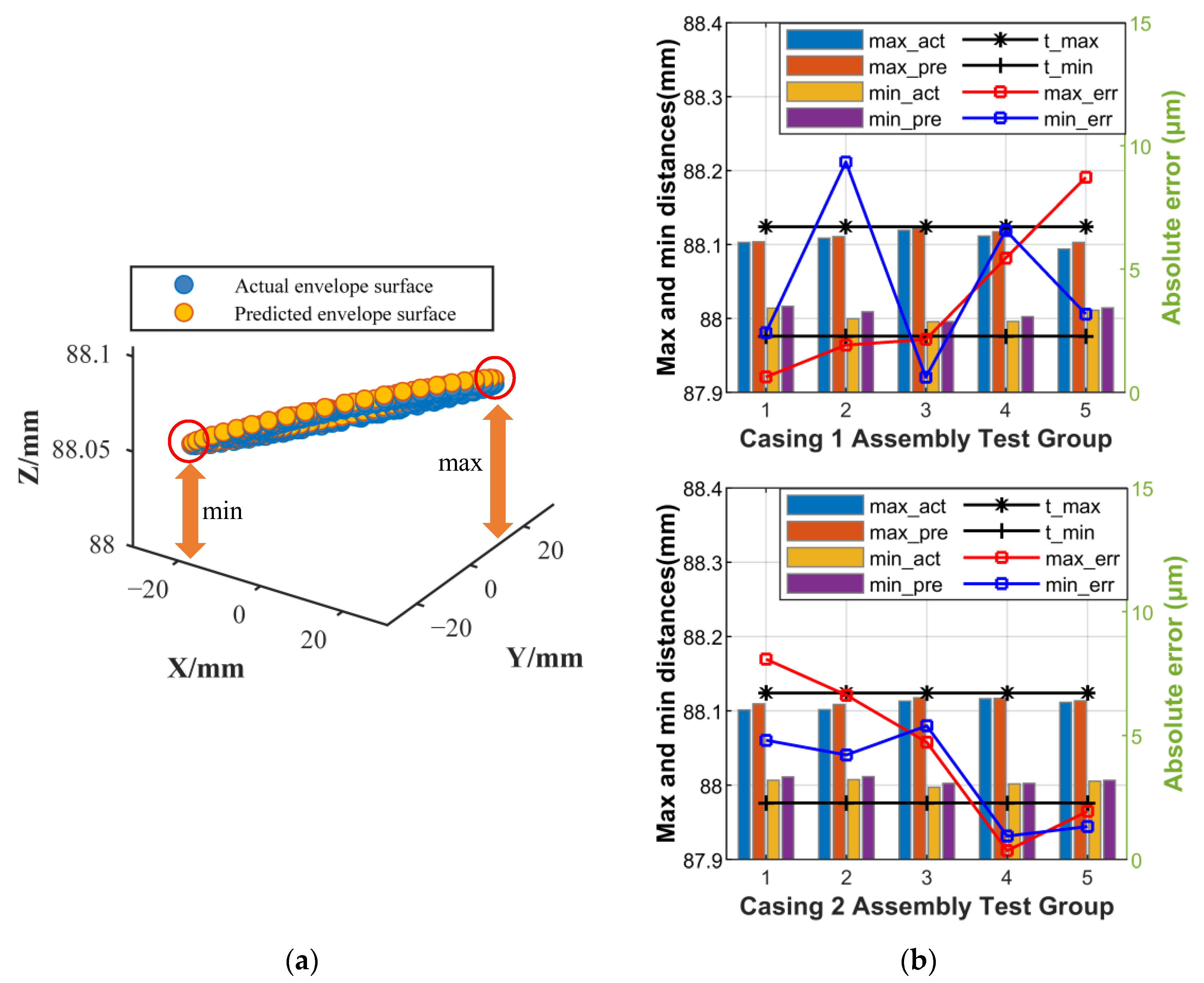
To demonstrate the multidimensional advantages of the SDC model, this subsection analyzes the prediction results using the following parameters. The predicted and actual envelope surfaces are shown in Figure 19, the maximum and minimum distances of the closed loop are presented in Figure 20, the parallelism in Figure 21, and the perpendicularity in Figure 22.

• Characterization results of the closed-loop datum plane

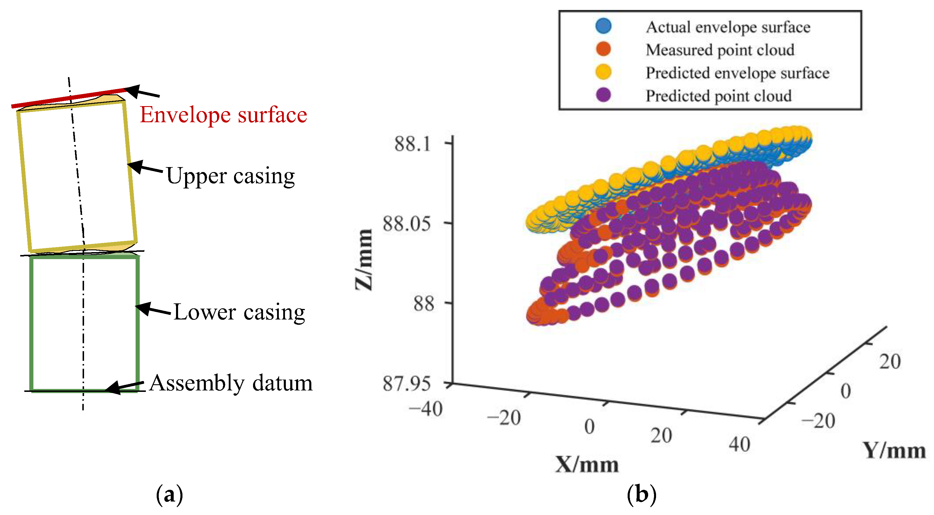
Figure 19 shows the state of the upper end face of casing 1 when rotated 0° clockwise around the z-axis in the assembly coordinate system (dataset 1 from the casing 1 assembly test group). The red point cloud represents the measured point cloud data, the blue point cloud represents the actual envelope surface obtained after characterization of the measured point cloud, the purple point cloud represents the predicted point cloud data obtained from the SDC model, and the yellow point cloud represents the predicted envelope surface after characterization of the predicted point cloud.

Characterizing parameters of the envelope surface: P_r1′ = {−0.0818, −0.0143, 88.0601, −0.0012, 0.0008, 1}

The characteristic equation is expressed as:

$$\left\{\begin{array}{c}(-0.0012)\times (x-(-0.0818))+0.0008\times (y-(-0.0143))+(z-88.0601)=0\\ x\in [-0.0818-31,-0.0818+31]\\ y\in [-0.0143-\sqrt{{{\displaystyle 31}}^2-{(x+0.0818)}^2},-0.0143+\sqrt{{{\displaystyle 31}}^2-{(x+0.0818)}^2}]\end{array}\right.$$

(14)

2.

Maximum and minimum distances of the closed loop

$$\left\{\begin{array}{c}max\_pre=max\left|Q{p}_i\right|;max\_act=max\left|Q{a}_j\right|;\\ max\_err=\left|max\left|Q{p}_i\right|-max\left|Q{a}_j\right|\right|;\\ min\_pre=min\left|Q{p}_i\right|;min\_act=min\left|Q{a}_j\right|;\\ min\_err=\left|min\left|Q{p}_i\right|-min\left|Q{a}_j\right|\right|,\end{array}\right.(i,j=1,2,\dots ,n)$$

(15)

where Qp_i—the z-coordinates of the predicted envelope point cloud; Qa_j—the z-coordinates of the actual envelope point cloud; max_pre—maximum value of Qp_i; max_act—maximum value of Qa_j; max_err—absolute error between max_pre and max_act; min_pre—minimum value of Qp_i; min_act—minimum value of Qa_j; min_err—absolute error between min_pre and min_act; n—number of verification points.

A comparison of the actual results of the envelope surface, the predicted results of the envelope surface, and the predicted values from the traditional worst-case dimension chain method (closed-loop dimensional errors range between t_min = 87.975 mm and t_max = 88.124 mm) is shown in Figure 20. The results obtained by the traditional worst-case dimension chain method remain unchanged regardless of the phase rotation of the upper casing. This is because the worst-case method yields a fixed interval range (a scalar value) that does not account for the distribution of form errors. In contrast, the spatial gap of the closed loop varies with the assembly phase shift between the upper and lower casings, demonstrating the advantage of the SDC model in providing multidimensional closed-loop results. The absolute errors between the predicted and actual values are all below 9.3 μm, further confirming the accuracy of the predictions. These findings provide a theoretical basis for optimizing tolerance design.

3.

Parallelism of the envelope surface

$$para\_per=\left|{\displaystyle \frac{para\_act-para\_pre}{para\_act}}\right|\times 100\%$$

(16)

where para_act denotes the parallelism of the actual envelope surface, par_pre denotes the parallelism of the predicted envelope surface, and para_per denotes the relative error between para_act and par_pre.

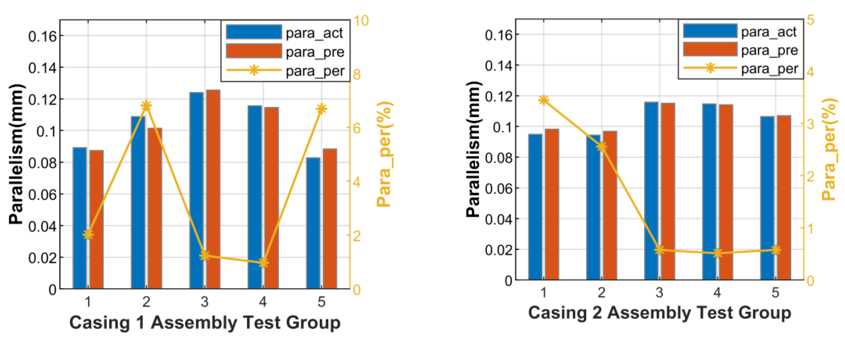
As shown in Figure 21, as the upper casing rotates relative to the lower casing, the parallelism of the closed loop varies, further demonstrating the advantage of the SDC model in dimensional characterization. Moreover, the relative error between the actual and predicted parallelism values remains below 6.8%, validating that the model’s predictions closely match the real results.

4.

Perpendicularity of the envelope surface

perpend_per = |perpend_act − perpend_pre|

(17)

where perpend_act denotes the perpendicularity of the actual envelope surface, perpend_pre denotes the perpendicularity of the predicted envelope surface, and perpend_per denotes the absolute error between perpend_act and perpend_pre.

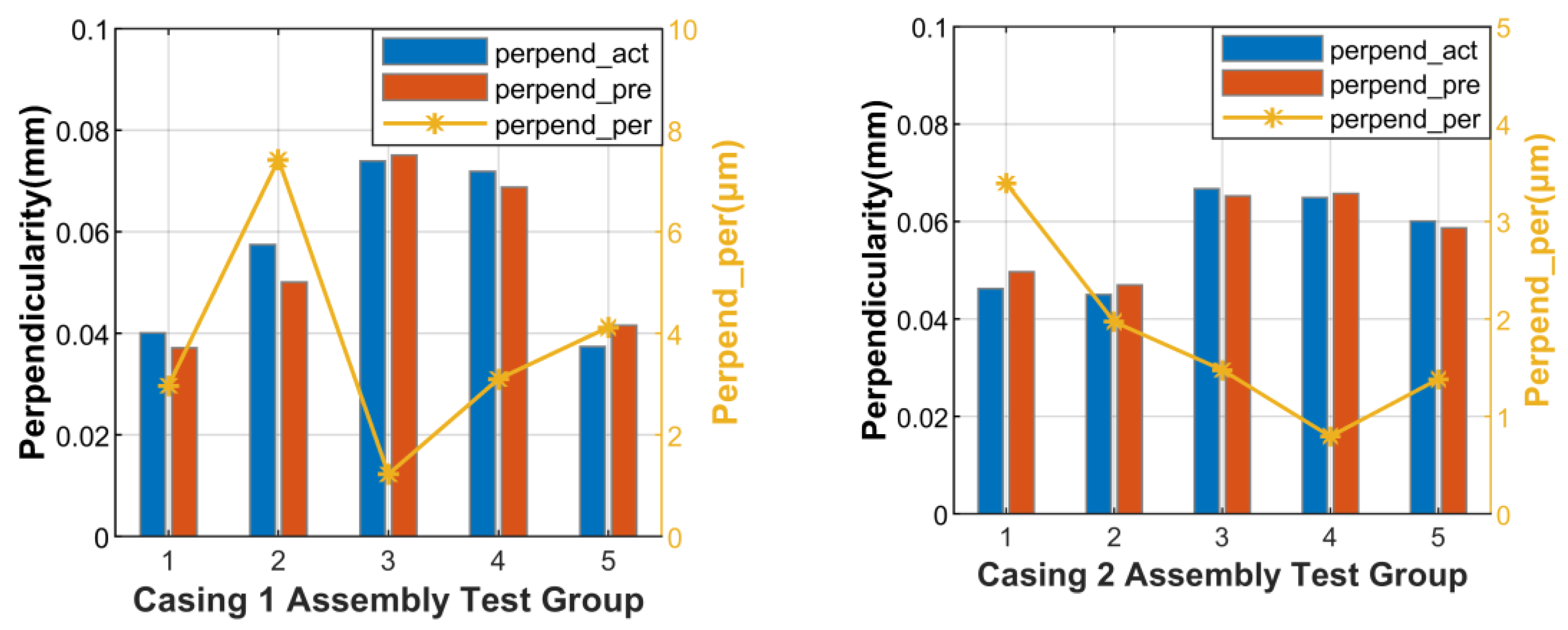
As shown in Figure 22, the perpendicularity of the envelope surface relative to the datum axis changes with the assembly phase variation between the upper and lower casings, further highlighting the SDC model’s advantage in dimensional characterization. Additionally, the relative error between the actual and predicted perpendicularity values remains below 7.4%, confirming the model’s prediction accuracy.

3.3.2. Effect of SMSC and MMSC on End Face Closed-Loop Accuracy

To validate the accuracy improvement of the spatial dimension chain-based multiple mating-surface constraint (SDC-MMSC) method for assembled structures with multiinterface constraints (Figure 15, showing the flange fitting between the lower casing’s top surface and the upper casing’s bottom surface), this subsection compares three parameters among the SDC-MMSC method, the spatial dimension chain-based single mating surface constraint (SDC-SMSC) method (simplifying multiple constraints to a single mating surface constraint), and experimental measurements:

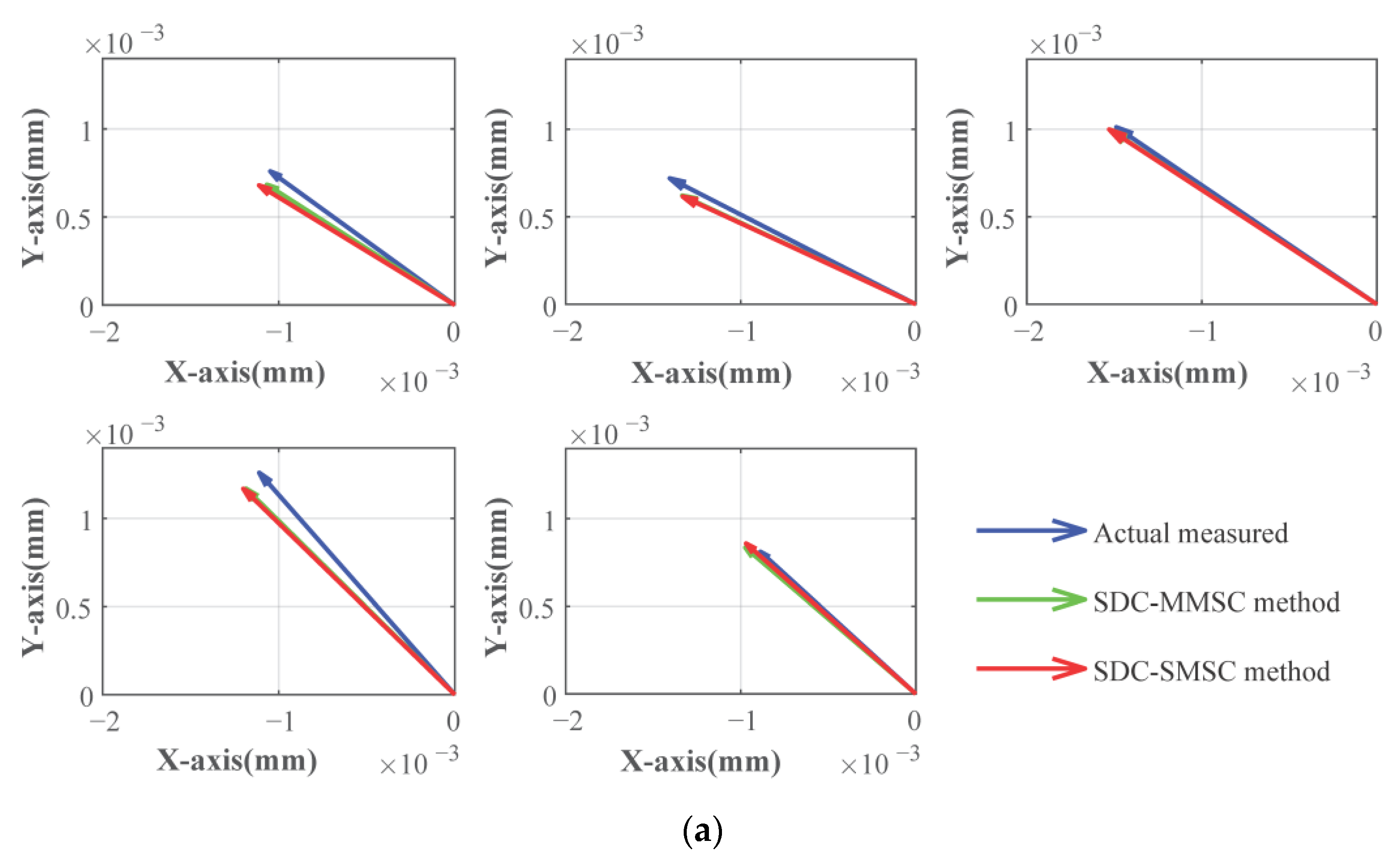
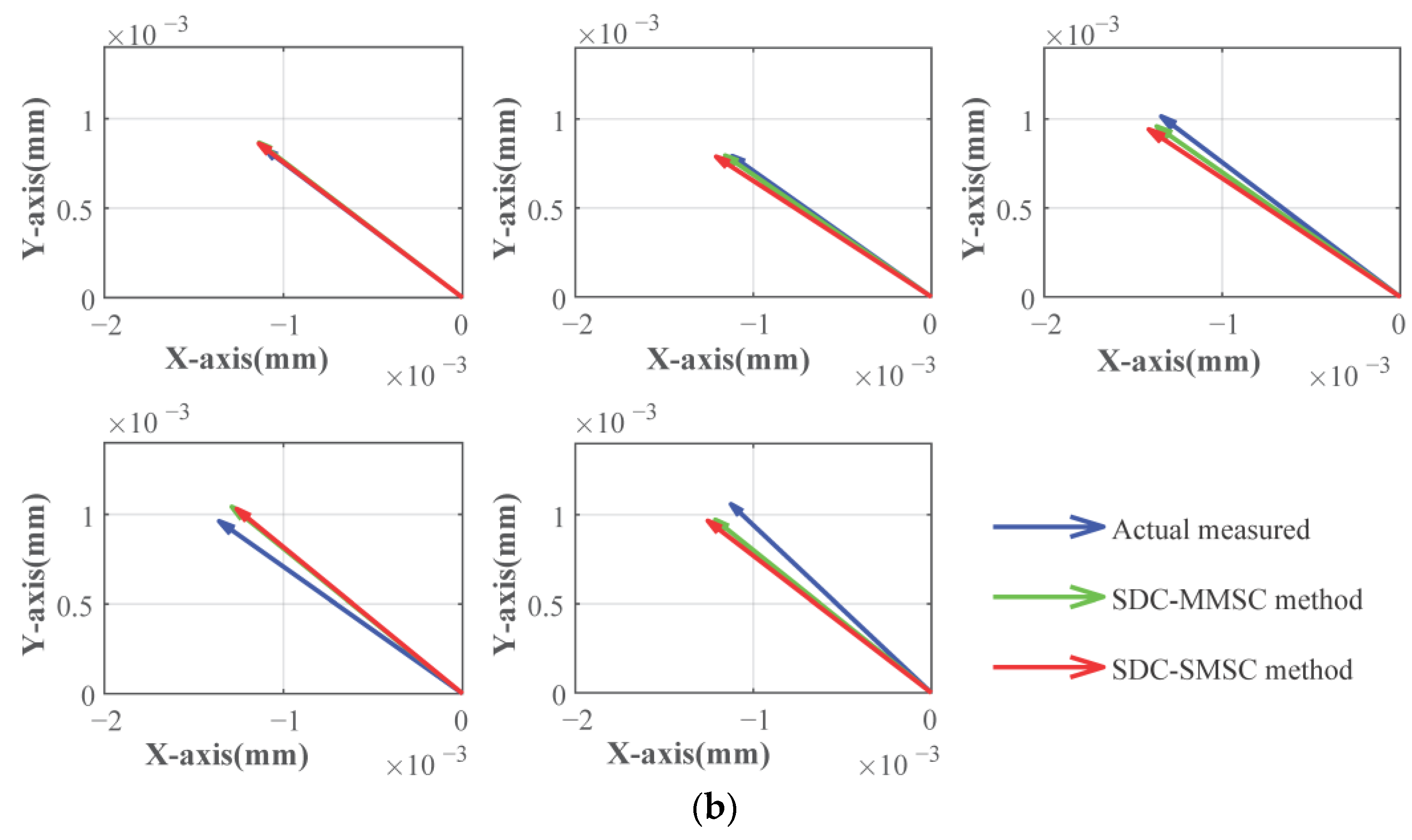
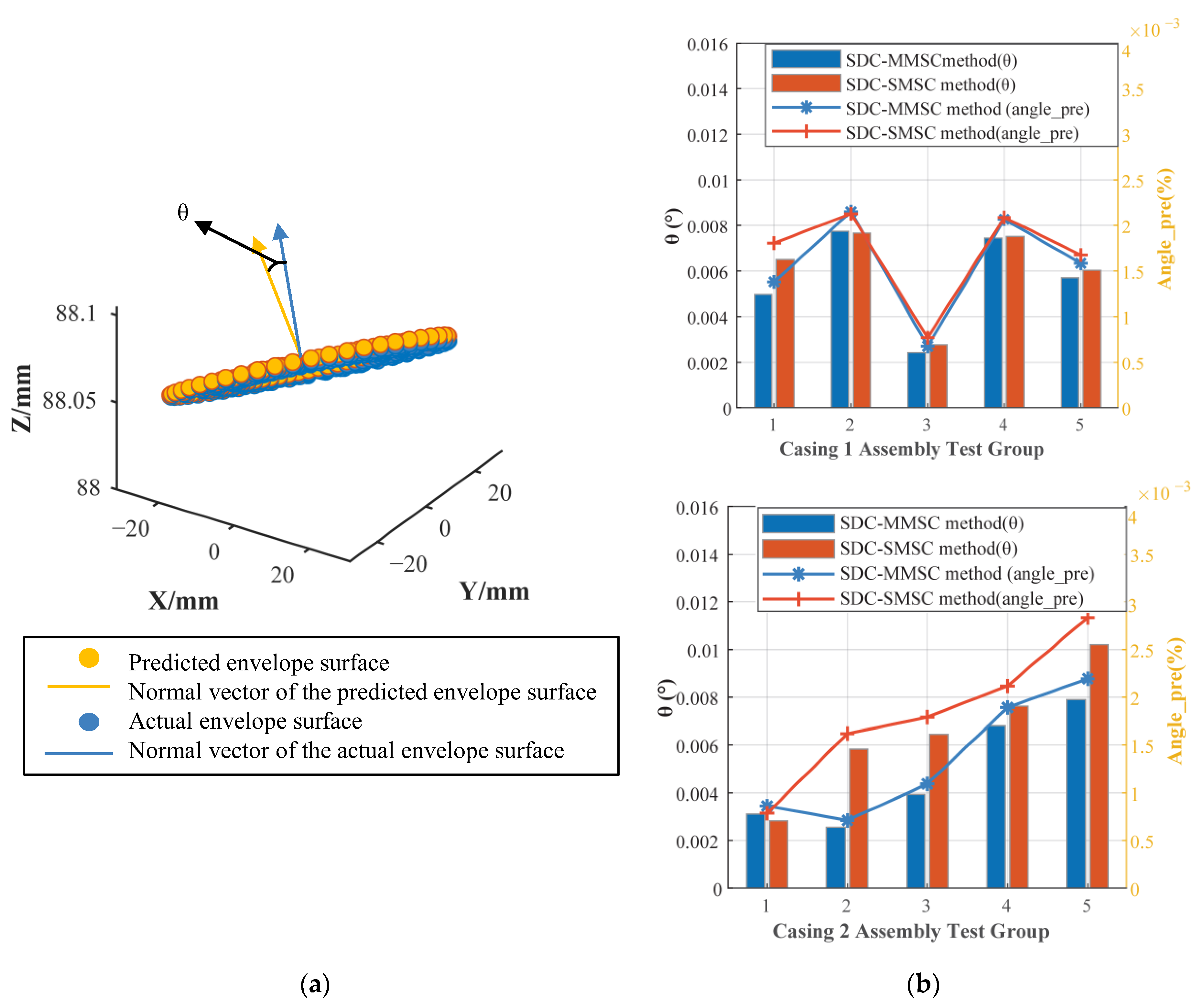
• The normal vector of the envelope surface (Figure 23);
• The angular error θ between the predicted and actual normal vectors (Figure 24);
• The root mean square error (RMSE) between the predicted and actual envelope surfaces (Figure 25).

Figure 23 shows that the influence of the two pairs of mating surfaces on dimensional chain accuracy cannot be neglected. From Figure 24b, the angular error θ obtained via the SDC-MMSC method remains below 0.008°. Among the 10 datasets, the SDC-MMSC method exhibits smaller relative errors than the SDC-SMSC method in 7 cases, while the two methods achieve comparable accuracy in the remaining 3 cases. Figure 25 indicates that the RMSE of the SDC-MMSC method remains below 0.006 mm, demonstrating its superior accuracy over the SDC-SMSC method. The experimental results confirm the method’s effectiveness and demonstrate that multiconstraint consideration significantly enhances the accuracy over existing techniques.

$$\left\{\begin{array}{c}\mathrm{Normal} \mathrm{vector} \mathrm{extraction} \mathrm{from} \mathrm{envelope} \mathrm{surfaces}:\min {\displaystyle \sum _{i=1}^K\frac{{(a{x}_i+b{y}_i+c{z}_i-d)}^2}{2}}\\ \theta =\arccos ({\displaystyle \frac{\overrightarrow{m}\cdot \overrightarrow{n}}{‖\overrightarrow{m}‖\cdot ‖\overrightarrow{n}‖}})\\ angle\_per=\left|{\displaystyle \frac{\theta }{360}}\right|\ast 100\%\end{array}\right.$$

(18)

where $\overrightarrow{m}=(a,b,c)$ is the normal vector of the plane, d is the constant term in the plane equation composed of K points, (x_i, y_i, z_i) represents the point cloud coordinates of the envelope surface, K is the number of point clouds, θ is the angle between two vectors, $\overrightarrow{m},\overrightarrow{n}$ denote two vectors, ||·|| represents the magnitude (norm) of a vector, and angle_pre is the relative error (normalized to 360°) between the predicted surface normal vector and the actual surface normal vector.

$$RMSE=\sqrt{{\displaystyle \sum _{s=1}^k\frac{{(P^E-P^{\prime })}^2}{k}}}=\sqrt{{\displaystyle \sum _{s=1}^k\frac{{(x_s-x_s^{\prime })}^2+{(y_s-y_s^{\prime })}^2+{(z_s-z_s^{\prime })}^2}{k}}}$$

(19)

where k denotes the number of measurement points, P^E = (x_s, y_s, z_s) represents the actual envelope surface, and P′ = (x_s′, y_s′, z_s′) denotes the predicted envelope surface.

3.3.3. Coaxiality Prediction in Axis-Based Closed Loop

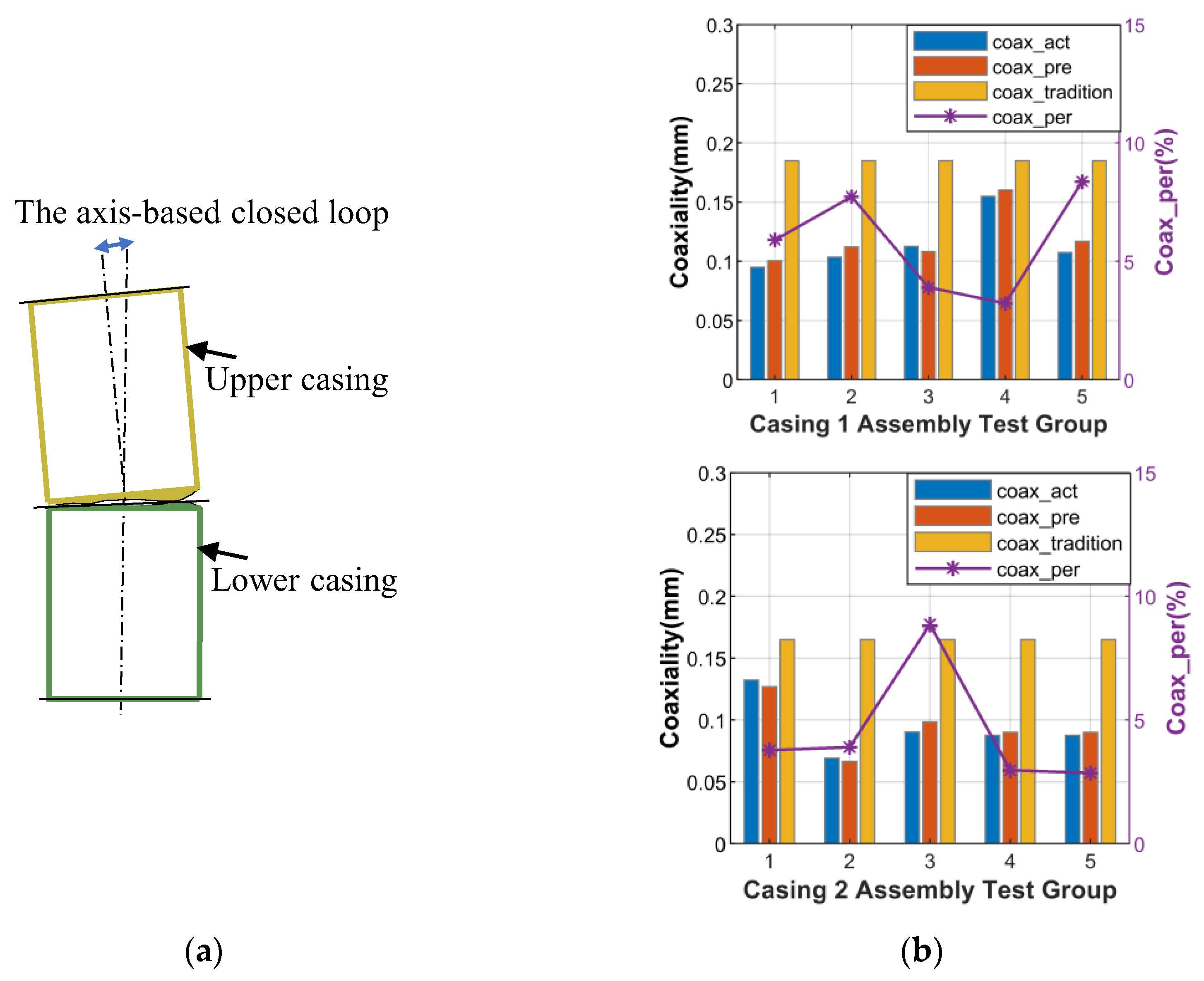
In practical engineering, secondary factors are often empirically neglected to simplify calculations. This study focuses on geometric errors of casing mating surfaces (e.g., flatness, parallelism) that significantly affect the coaxiality. By substituting the characteristic parameters into Equations (11) and (12), Equation (13) is derived, representing the spatial six-dimensional (position and orientation vectors) distribution of a pair of datum axes in the axis-based closed loop. This subsection validates the accuracy of the SDC model through the coaxiality metric (Equation (20)), comparing the dimension chain worst-case method, the proposed model’s predictions, and experimental results, as shown in Figure 26.

$$coax\_per=\left|{\displaystyle \frac{coax\_act-coax\_pre}{coax\_act}}\right|\times 100\%$$

(20)

where coax_act denotes the actual coaxiality, coax_pre represents the predicted coaxiality, and coax_per is the relative error between the predicted and actual coaxiality.

A comparative analysis was conducted between the predicted values from the axis-based closed-loop model and actual measured values, along with results from the worst-case assembly dimension chain method. As illustrated, due to differences in the assembly phase between the upper and lower casings, the coaxiality also varies. This further demonstrates that spatially distributed form errors cannot be neglected in the SDC model. Moreover, the relative error between the predicted and actual coaxiality is less than 8.3% in all cases and consistently smaller than the results obtained using the traditional worst-case dimension chain method (coaxiality errors of 0.185 mm for casing 1 test group and 0.165 mm for casing 2 test group). These results validate that the predictions of the proposed model closely align with the actual measurements.

4. Application of SDC Model for Tolerance Allocation Optimization

The effectiveness of the SDC model has been experimentally validated in the previous section using an engine casing case study. The ultimate goal of constructing this model is to enable more precise tolerance allocation in design. Taking the engine casing from Section 3 as an example, the application steps of the SDC model are as follows:

• Define the assembly’s functional requirements: The parallelism of the envelope surface derived from the upper casing’s top face must be ≤0.03 mm.
• Identify contributing loops: The specific parameters are illustrated in Figure 15.
• Assign tolerances: Based on design experience and process capability, tolerances are allocated to each contributing loop (see case 1).
• Establish the SDC model: Based on the tolerance range defined in step 3, previously machined casings within this tolerance are inspected. Systematic errors are extracted and separated using NURBS-based surface regression [35], serving as the error component in the SDC model. The actual mating-constrained datum surface and non-mating-constrained datum surface are characterized, and their respective errors (M and N) are solved. The SDC model is then established, followed by Monte Carlo simulation.
  A critical point is that form tolerances must comply with orientation tolerances; for instance, in design and simulation, the generated form errors (e.g., flatness) must be smaller than the corresponding orientation errors (e.g., parallelism).
  To elucidate the connection between steps 3 and 4, we provide illustrative examples that demonstrate their interrelationship in the geometric error generation process.

  (1)

  Form Error (e.g., Flatness)

  Evaluation method: Two parallel planes minimally enclose the actual surface (minimum zone method).

  (2)

  Orientation Error (e.g., Parallelism)

  Evaluation method: First, an ideal reference plane is fitted from the measured datum surface using a mathematical method such as least squares regression. Second, the maximum vertical deviation of all measured surface points from this reference plane is calculated, which defines the parallelism error value.

  (3)

  Generating Form Errors (e.g., Flatness)

  (a)

  Assign a flatness error magnitude V.

  (b)

  Incorporate the error distribution pattern from existing manufacturing processes.

  (c)

  Scale the Z-coordinates of measured point clouds:

  $$Z_{new}=Z_{ori}\times {\displaystyle \frac{V}{V_{ori}}}$$

  (21)

  where $Z_{ori}$ denotes the original coordinate; $V_{ori}$ denotes the measured flatness error.

  (4)

  Generating Orientation Errors (e.g., Parallelism)

  (a)

  Assign a parallelism error magnitude.

  (b)

  Rotate the form-corrected point cloud (about the x-axis, y-axis, or both axes) to control the quadrant of maximum Z-deviation.

  (5)

  Monte Carlo Simulation Workflow

  (a)

  Set tolerances for all relevant part surfaces.

  (b)

  Randomly sample error magnitudes within tolerance limits and generate corresponding error point clouds.

  (c)

  Map geometric features to functional dimensions using the 6-DOF vector function.

  (d)

  Calculate the functional parameters (e.g., assembly clearance)

  (e)

  Determine the batch assembly yield.

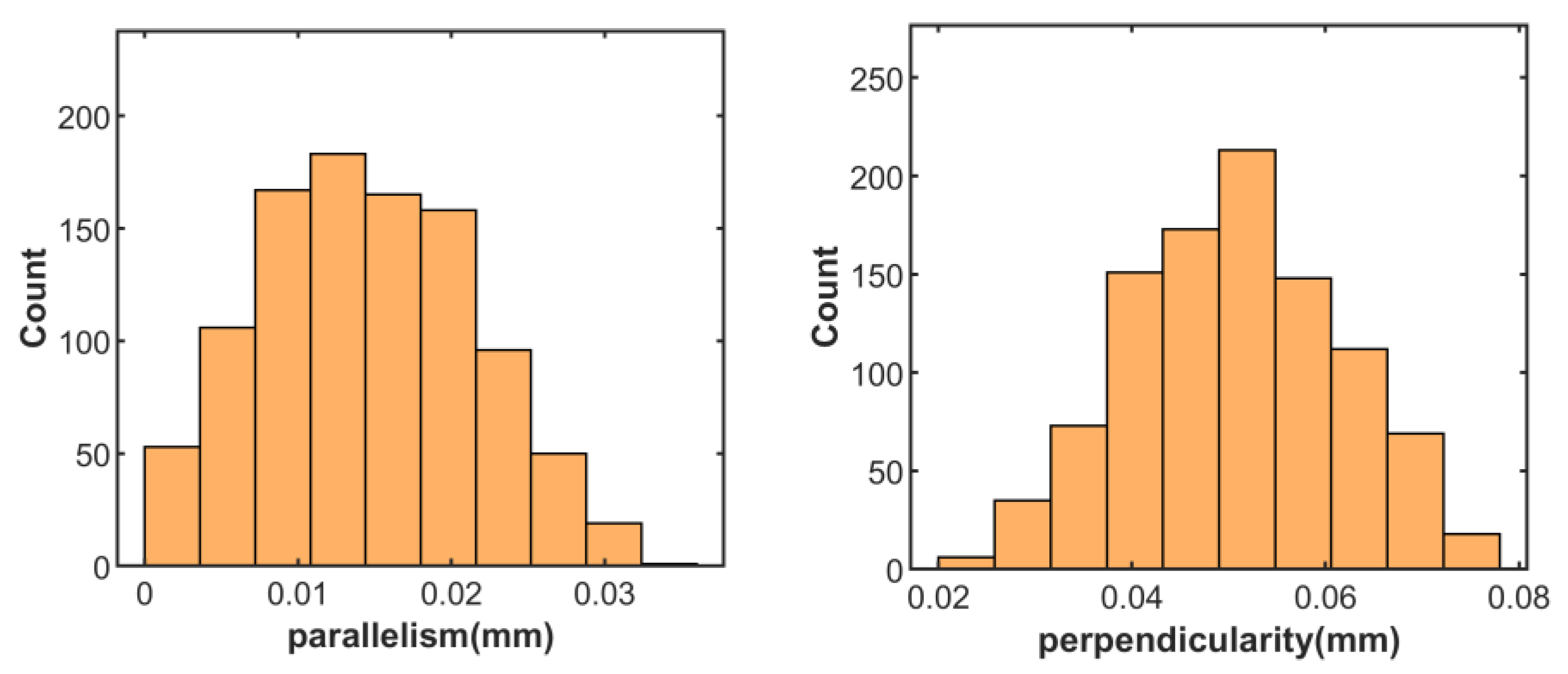
• Validate the tolerance design: For example, the rationality can be evaluated by assessing whether the compliance rate of positional errors (e.g., parallelism or perpendicularity) in the datum plane of the closed loop meets the design requirements. As shown in Figure 27, the parallelism of the envelope surface falls within [0, 0.025] mm with a 93% compliance rate, confirming compliance with the ≤0.03 mm requirement.
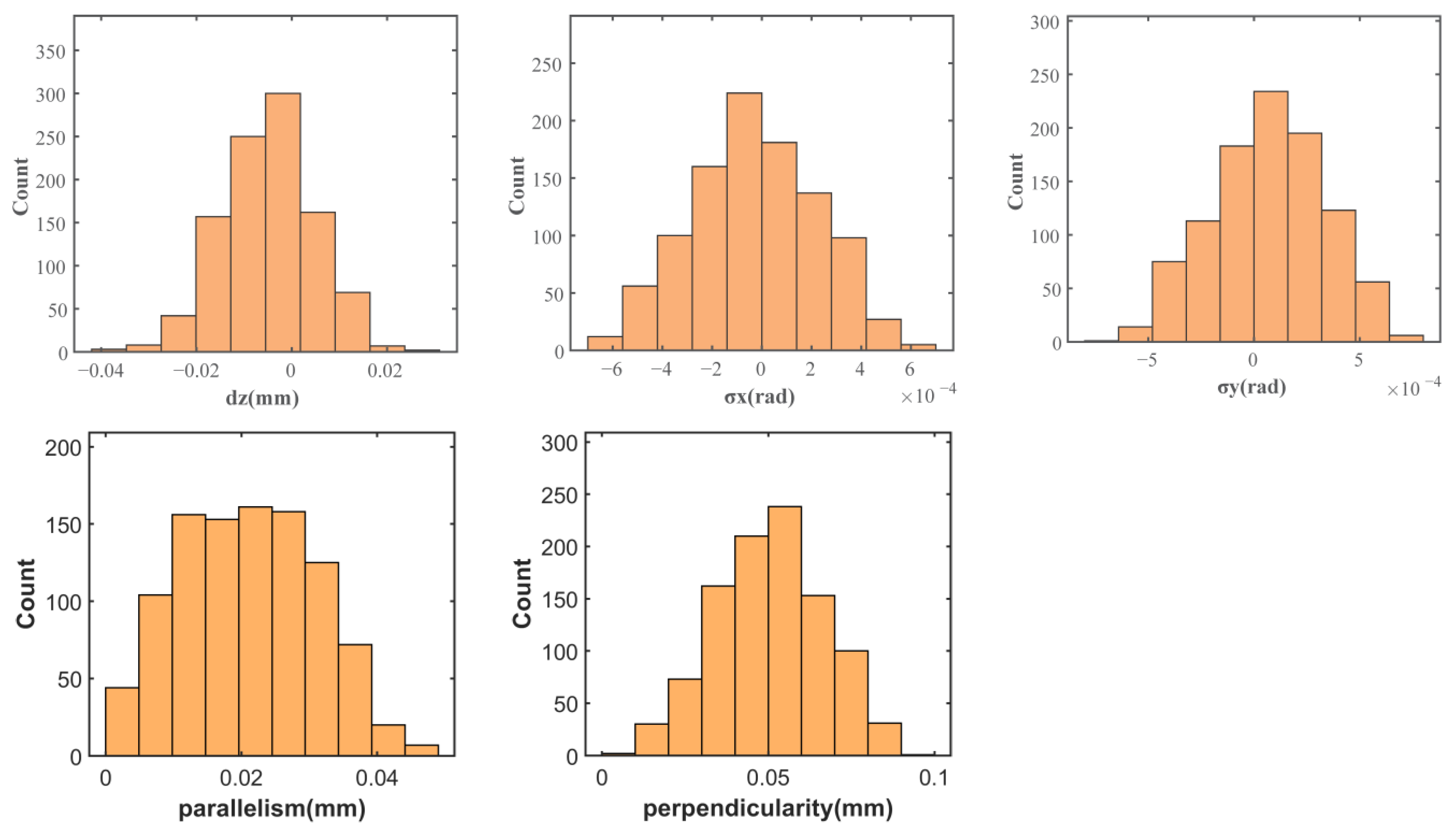
• Optimize the tolerances: Adjust the tolerances with lower process costs to improve the product accuracy and reduce manufacturing expenses. For instance, if the dimensional or parallelism tolerances of the upper or lower casings are overly stringent (leading to high machining costs), they can be relaxed per case 2. Repeating step 4 yields the results in Figure 28, where the parallelism within [0, 0.029] mm achieves a 78% compliance rate. If acceptable, this relaxation maintains precision while lowering costs.

The advantages of using the SDC model for tolerance allocation include:

• Cost reductions: Loosening the tolerances where possible without compromising assembly requirements reduces the machining costs.
• Design optimization: Refining the tolerance allocation process via the distributed-form-error-based SDC model enhances the part design accuracy.

The simulation parameters used in the above steps were as follows.

The error magnitudes were sampled based on a normal distribution within the tolerance range, and the spatially distributed form errors were characterized based on experimental measurement data from existing manufacturing processes. The perpendicularity datum axis was constructed based on measured data from the inner cylinder of the casing, and the basic dimensional parameters of the contributing loops are shown in Figure 17. After 1000 simulation runs, the pose errors [dz, σx, σy] of the envelope surface at different tolerance grades were obtained, along with the parallelism and perpendicularity.

Case 1: As previously discussed, the geometric errors in the upper end face of the lower casing and both end faces of the upper casing are critical factors influencing the closed loop. The specific parameters are as follows: dimensional tolerance [−0.011, 0.014] mm, positional tolerance (parallelism) [0, 0.02] mm, and form tolerance (flatness) [0, 0.01] mm. Regarding the simulation results, the displacement in the z-direction is primarily distributed within the range of [−0.014, −0.006] mm, with 492 data points. The rotational error about the x-axis is mainly distributed within [−0.00016, 0.00017] rad, with 604 data points, while the rotational error about the y-axis is mainly distributed within [0.00005, 0.00015] rad, with 411 data points. The parallelism of the envelope surface achieves a compliance rate of 93% within the [0, 0.025] mm range, whereas the perpendicularity compliance rate is 79% within the [0, 0.06] mm range. The result distribution is illustrated in Figure 27.

Case 2: Similarly, the tolerance parameters for the three surfaces, the upper end face of the lower casing and the upper and lower end faces of the upper casing, are specified as follows: dimensional tolerance of [−0.015, 0.024] mm, positional tolerance (parallelism) of [0, 0.03] mm, and form tolerance (flatness) of [0, 0.015] mm. The displacement z is predominantly distributed within [−0.0128, −0.0055] mm, with 550 data points. The rotational error about the x-axis is mainly distributed in [−0.00028, 0.00014] rad, with 565 data points, while the rotational error about the y-axis is primarily within [−0.00016, 0.00032] rad, with 612 data points. The parallelism of the envelope surface yields a 62% compliance rate within [0, 0.0245] mm, 78% within [0, 0.029] mm, and 90% within [0, 0.034] mm. The perpendicularity achieves a 71.5% compliance rate within [0,0.06] mm. The result distribution is illustrated in Figure 28.

5. Conclusions and Future Work

This study established an advanced framework for precision tolerance design, with the core innovation being the development of a six-dimensional SDC model. The effectiveness of the SDC model was validated through an assembly case study using simulated aero-engine casings. The main conclusions are as follows:

(1) A six-dimensional SDC model was developed, which integrates spatially distributed form errors into datum definitions using the transfer matrix theory. By employing six-dimensional vector functions (combining position and orientation parameters), the model achieves high-fidelity mapping between geometric features and functional dimensions, enabling accurate closed-loop predictions for large-scale assemblies.

(2) The six-dimensional SDC model systematically addresses complex constraint scenarios through a hierarchical approach. For the SMSC, the model characterizes spatially distributed form errors by deriving 6-DoF geometric error components through optimized algorithms, thereby enhancing the prediction accuracy. The solution extends to MMSC interactions by characterizing 3D coupled errors through 6-DoF components, effectively reducing the computational complexity while improving the prediction accuracy. Additionally, a novel non-mating-constrained datum plane error characterization method based on modified envelope conditions ensures assembly interchangeability.

(3) Assembly experiments using simulated aero-engine casings demonstrated that all measured values satisfied worst-case dimension chain tolerance limits. Furthermore, the closed-loop spatial distances varied with the assembly phase difference between the upper and lower casings, conclusively validating the necessity of considering spatially distributed form errors in SDC modeling and their multidimensional characteristics. A comparative analysis between the SDC-SMSC and SDC-MMSC methods further confirmed the superiority of the multiconstraint approach.

The model is applicable to planar mating assemblies where surfaces cannot be simplified as points or beams for analyses, enabling error prediction and tolerance allocation during the design phase. Our future work will extend the methodology to curved surface mating assemblies, enhancing its industrial applicability. This research provides both theoretical foundations and practical solutions for the precision assembly and cost-effective manufacturing of complex mechanical systems.

References

1. Dantan, J.; Homri, L. Overview of mathematical concepts for tolerance analysis. Procedia CIRP 2024, 129, 73–78. [Google Scholar] [CrossRef]
2. Jiang, Q.J.Q.; Feng, H.F.H.; Wang, Y.W.Y.; Fang, C.F.C. Batch circular form error characterization and evaluation. Precis. Eng. 2017, 47, 223–230. [Google Scholar] [CrossRef]
3. Dantan, J.Y.; Qureshi, A.J. Worst-case and statistical tolerance analysis based on quantified constraint satisfaction problems and Monte Carlo simulation. Comput. Aided Des. 2009, 41, 1–12. [Google Scholar] [CrossRef]
4. Mansuy, M.; Giordano, M.; Hernandez, P. A new calculation method for the worst case tolerance analysis and synthesis in stack-type assemblies. Comput. Aided Des. 2011, 43, 1118–1125. [Google Scholar] [CrossRef]
5. Mansuy, M.; Giordano, M.; Hernandez, P. A Generic Method for the Worst Case and Statistical Tridimensional Tolerancing Analysis. Proc. CIRP 2013, 10, 276–282. [Google Scholar] [CrossRef]
6. Sahani, A.K.; Jain, P.K.; Sharma, S.C.; Bajpai, J.K. Design Verification through Tolerance Stack up Analysis of Mechanical Assembly and Least Cost Tolerance Allocation. Procedia Mater. Sci. 2014, 6, 284–295. [Google Scholar] [CrossRef]
7. Bhide, S.; Davidson, J.K.; Shah, J.J. Areal Coordinates: The Basis of a Mathematical Model for Geometric Tolerances. Geom. Prod. Spec. Verif. Funct. Integr. 2003, 35–44. [Google Scholar] [CrossRef]
8. Davidson, J.K.; Shah, J.J. Geometric tolerances: A new application for line geometry and screws. Proc. Inst. Mech. Eng. Part C J. Mech. Eng. Sci. 2020, 216, 95–104. [Google Scholar] [CrossRef]
9. Mujezinovic, A.; Davidson, J.K.; Shah, J.J. A New Mathematical Model for Geometric Tolerances as Applied to Polygonal Faces. J. Mech. Des. 2003, 126, 504–518. [Google Scholar] [CrossRef]
10. Chase, K.W.; Gao, J.; Magleby, S.P.; Sorensen, C.D. Including Geometric Feature Variations in Tolerance Analysis of Mechanical Assemblies. IIE Trans. 1996, 28, 795–807. [Google Scholar] [CrossRef]
11. Chase, K.; Magleby, S.; Glancy, C.; Chase, K.; Magleby, S.; Glancy, C.; Chase, K.; Magleby, S.; Glancy, C. A Comprehensive System for Computer-Aided Tolerance Analysis of 2-D and 3-D Mechanical Assemblies. In Geometric Design Tolerancing: Theories, Standards and Applications; Springer Nature: Berlin/Heidelberg, Germany, 1998; pp. 294–307. [Google Scholar] [CrossRef]
12. Chase, K.W.; Gao, J.; Magleby, S.P. General 2-D Tolerance Analysis of Mechanical Assemblies with Small Kinematic Adjustments. J. Design Manuf. 1995, 5, 263–274. [Google Scholar]
13. Gao, J.; Chase, K.W.; Magleby, S.P. Generalized 3-D tolerance analysis of mechanical assemblies with small kinematic adjustments. IIE Trans. 1998, 30, 367–377. [Google Scholar] [CrossRef]
14. Clément, A.; Desrochers, A.; Rivière, A. Theory and Practice of 3-D Tolerancing for Assembly. In Proceeding of CIRP Seminar on Computer Aided Tolerancing; Penn State University: University Park, PA, USA, 1991; Volume 25. [Google Scholar]
15. Clément, A.; Bourdet, P. A Study of Optimal-Criteria Identification Based on the Small-Displacement Screw Model. CIRP Ann. Manuf. Technol. 1988, 37, 503–506. [Google Scholar] [CrossRef]
16. Desrochers, A. Modeling Three Dimensional Tolerance Zones Using Screw Parameters. In Proceedings of the ASME 1999 Design Engineering Technical Conferences, Las Vegas, NV, USA, 12–16 September 1999; pp. 895–903. [Google Scholar]
17. Desrochers, A.; Clément, A. A dimensioning and tolerancing assistance model for CAD/CAM systems. J. Adv. Manuf. Technol. 1994, 9, 352–361. [Google Scholar] [CrossRef]
18. Laifa, M.; Sai, W.B.; Hbaieb, M. Evaluation of machining process by integrating 3D manufacturing dispersions, functional constraints, and the concept of small displacement torsors. Int. J. Adv. Manuf. Technol. 2014, 71, 1327–1336. [Google Scholar] [CrossRef]
19. Legoff, O.; Villeneuve, F.; Bourdet, P. Geometrical tolerancing in process planning: A tridimensional approach. Proc. Inst. Mech. Eng. Part B-J. Eng. Manuf. 1999, 213, 635–640. [Google Scholar] [CrossRef]
20. Teissandier, D.; Couétard, Y.; Gérard, A. A computer aided tolerancing model: Proportioned assembly clearance volume. Comput. Aided Des. 1999, 31, 805–817. [Google Scholar] [CrossRef]
21. Desrochers, A.; Rivière, A. A matrix approach to the representation of tolerance zones and clearances. Int. J. Adv. Manuf. Technol. 1997, 13, 630–636. [Google Scholar] [CrossRef]
22. Wang, H.; Ning, R.; Tang, C. Automatic generation of 3D as sembly dimension chains. Chin. J. Mech. Eng. 2005, 41, 7. [Google Scholar] [CrossRef]
23. El Mouden, M.; Chahbouni, M.; Boutahari, S. A New Approach for Synthesis of 3D Tolerances with Consideration of Flatness Defects in Mechanical Assembly Using Jacobian Torsor Model. Int. J. Eng. Appl. 2024, 12, 169–179. [Google Scholar] [CrossRef]
24. Zhang, J.; Qiao, L. Three Dimensional Manufacturing Tolerance Design Using Convex Sets. Procedia CIRP 2013, 10, 259–266. [Google Scholar] [CrossRef]
25. Jain, P. Unified approach for tolerance analysis, synthesis, and compensator selection. Appl. Optics 2022, 61, 8974–8981. [Google Scholar] [CrossRef]
26. Tang, W.; Xu, G.; Zhang, S. Dimensional Variation Analysis for Rigid Part Assembly With an Improvement of Monte Carlo Simulation. IEEE Access 2020, 8, 5862–5872. [Google Scholar] [CrossRef]
27. Rausch, C.; Nahangi, M.; Haas, C.; Liang, W. Monte Carlo simulation for tolerance analysis in prefabrication and offsite construction. Autom. Constr. 2019, 103, 300–314. [Google Scholar] [CrossRef]
28. McGregor, D.J.; Bimrose, M.V.; Shao, C.; Tawfick, S.; King, W.P. Using machine learning to predict dimensions and qualify diverse part designs across multiple additive machines and materials. Addit. Manuf. 2022, 55, 102848. [Google Scholar] [CrossRef]
29. Maltauro, M.; Meneghello, R.; Concheri, G. Enhancing tolerance stack-up analysis with variable-dependent admissible limits. CIRP Ann. 2025, in press. [Google Scholar] [CrossRef]
30. Zhang, Q.; Jin, X.; Liu, Z.; Zhang, Z.; Fang, Y.; Zhang, Z.; Ledoux, Y. A New Approach of Surfaces Registration Considering Form Errors for Precise Assembly. Assem. Autom. 2018, 40, 789–800. [Google Scholar] [CrossRef]
31. Zhang, Q.; Jin, X.; Zhang, Z.; Zhang, Z.; Shang, K. Assembly Method Based on Constrained Surface Registration. J. Mech. Eng. 2018, 54, 70–76. [Google Scholar] [CrossRef]
32. Liu, T.; Zhao, Q.; Cao, Y.; Yang, J. A generic approach for analysis of mechanical assembly. Precis Eng. 2018, 54, 361–370. [Google Scholar] [CrossRef]
33. Shi, S.; Liu, J.; Gong, H.; Shao, N.; Anwer, N. Assembly accuracy analysis and phase optimization of aero-engine multistage rotors considering surface morphology and non-uniform contact deformation. Precis. Eng. 2024, 88, 595–610. [Google Scholar] [CrossRef]
34. Guo, H.; Zhang, Z.; Xiao, M.; Liu, H.; Zhang, Q. Tolerance optimization method based on flatness error distribution. Int. J. Adv. Manuf. Tech. 2021, 113, 1–15. [Google Scholar] [CrossRef]
35. Zhang, Z.; Zhang, Z.; Jin, X.; Zhang, Q. A novel modelling method of geometric errors for precision assembly. Int. J. Adv. Manuf. Technol. 2018, 94, 1139–1160. [Google Scholar] [CrossRef]
36. Anwer, N.; Schleich, B.; Mathieu, L.; Wartzack, S. From solid modelling to skin model shapes: Shifting paradigms in computer-aided tolerancing. CIRP Ann. Manuf. Technol. 2014, 63, 137–140. [Google Scholar] [CrossRef]
37. Corrado, A.; Polini, W.; Moroni, G.; Petrò, S. 3D Tolerance Analysis with Manufacturing Signature and Operating Conditions. In Proceedings of the 14th CIRP CAT 2016—CIRP Conference on Computer Aided Tolerancing, Gothenburg, Sweden, 18–20 May 2016; Volume 43, pp. 130–135. [Google Scholar]
38. Qie, Y.; Srinivasan, V.; Anwer, N. On Skin Model Describability using Laplace-Beltrami Operator for Geometrical Product Specification and Verification. Procedia CIRP 2024, 129, 67–72. [Google Scholar] [CrossRef]
39. Humienny, Z. Can ISO GPS and ASME Tolerancing Systems Define the Same Functional Requirements? Appl. Sci. 2021, 11, 8269. [Google Scholar] [CrossRef]
40. Shen, T.; Lu, C. An assembly accuracy analysis approach of mechanical assembly involving parallel and serial connections considering form defects and local surface deformations. Precis Eng. 2024, 88, 44–64. [Google Scholar] [CrossRef]
Figure 1. Effects of spatially distributed form errors.
Machines 13 00545 g001
Figure 2. Influence of spatially distributed form errors on the functional dimension (casing assembly coaxiality).
Machines 13 00545 g002
Figure 3. Influence of spatially distributed form errors on the functional dimension (shim thickness).
Machines 13 00545 g003
Figure 4. Spatial multidimensional distribution characteristics of the closed loop.
Machines 13 00545 g004
Figure 5. Datum for SDC modeling.
Machines 13 00545 g005
Figure 6. Relationship between global and local coordinate systems of critical surfaces.
Machines 13 00545 g006
Figure 7. Construction and application of SDC model.
Machines 13 00545 g007
Figure 8. Modeling mechanism for six-dimensional SDC.
Machines 13 00545 g008
Figure 9. SDC model.
Machines 13 00545 g009
Figure 10. Schematic of mating-constrained and non-mating-constrained datum errors.
Machines 13 00545 g010
Figure 11. Types of mating-constrained datum planes.
Machines 13 00545 g011
Figure 12. Characterization flowchart for mating-constrained datum errors.
Machines 13 00545 g012
Figure 13. Schematic of envelope plane characterization for actual non-mating-constrained datum planes.
Machines 13 00545 g013
Figure 14. Flowchart for solving envelope surface and non-mating-constrained datum errors.
Machines 13 00545 g014
Figure 15. End face closed-loop SDC in simulated casing assembly: (a) schematic of simulated casing assembly; (b) datum coordinate system construction and error contributors.
Machines 13 00545 g015
Figure 16. Axis-based closed-loop SDC in simulated casing assembly: (a) schematic of simulated casing assembly; (b) datum coordinate system construction and error contributors.
Machines 13 00545 g016
Figure 17. (a) Casing component diagram and (b) casing assembly diagram.
Machines 13 00545 g017
Figure 18. (a) Component measurement and (b) assembly measurement.
Machines 13 00545 g018
Figure 19. (a) Schematic diagram of parameter physical locations and (b) comparison of measured and predicted data (point clouds and envelope surfaces).
Machines 13 00545 g019
Figure 20. (a) Definition schematic and (b) comparison of actual vs. predicted maximum and minimum distances of the closed loop.
Machines 13 00545 g020
Figure 21. Comparison of actual vs. predicted parallelism of the envelope surface.
Machines 13 00545 g021
Figure 22. Comparison of actual vs. predicted perpendicularity of the envelope surface.
Machines 13 00545 g022
Figure 23. Comparison between predicted normal vectors (SDC-MMSC/SDC-SMSC methods) and actual measurements on envelope surfaces: (a) casing 1 test group; (b) casing 2 test group.
Machines 13 00545 g023aMachines 13 00545 g023b
Figure 24. Angular error (θ) between predicted and actual normal vectors: (a) definition schematic; (b) comparison between SDC-MMSC and SDC-SMSC methods.
Machines 13 00545 g024
Figure 25. RMSE between predicted and actual envelope surfaces.
Machines 13 00545 g025
Figure 26. Coaxiality comparison in axis-based closed loop: (a) schematic of axis-based closed loop; (b) predicted vs. measured coaxiality.
Machines 13 00545 g026
Figure 27. Distributions of the rotational errors (X/Y), translational error (Z), parallelism, and perpendicularity for the envelope surface in case 1.
Machines 13 00545 g027aMachines 13 00545 g027b
Figure 28. Distributions of the rotational errors (X/Y), translational Error (Z), parallelism, and perpendicularity for the envelope surface in case 2.
Machines 13 00545 g028