
Research on Robot Force Compensation and Collision Detection Based on Six-Dimensional Force Sensor


Abstract

1. Introduction
2. Theoretical Analysis
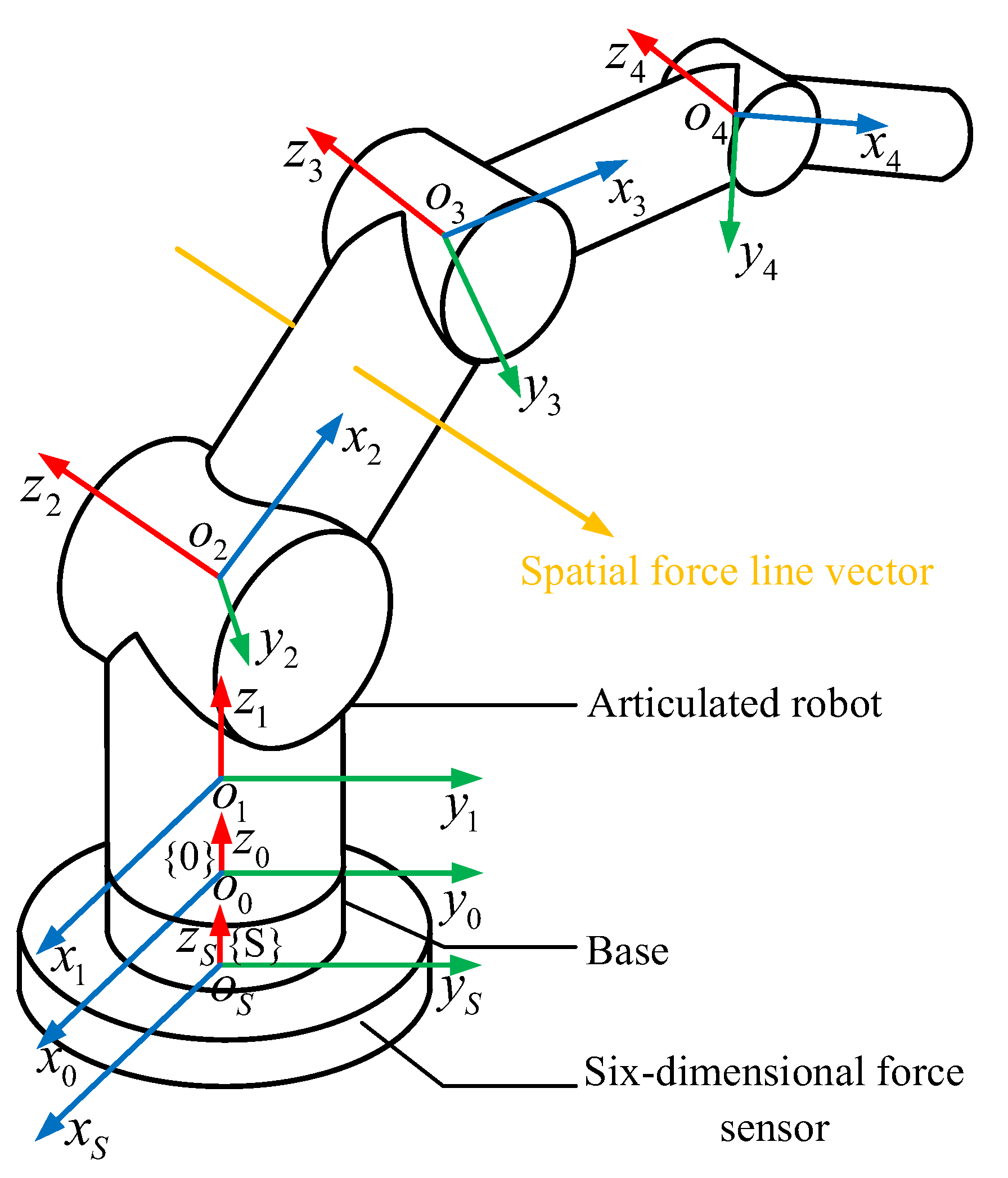
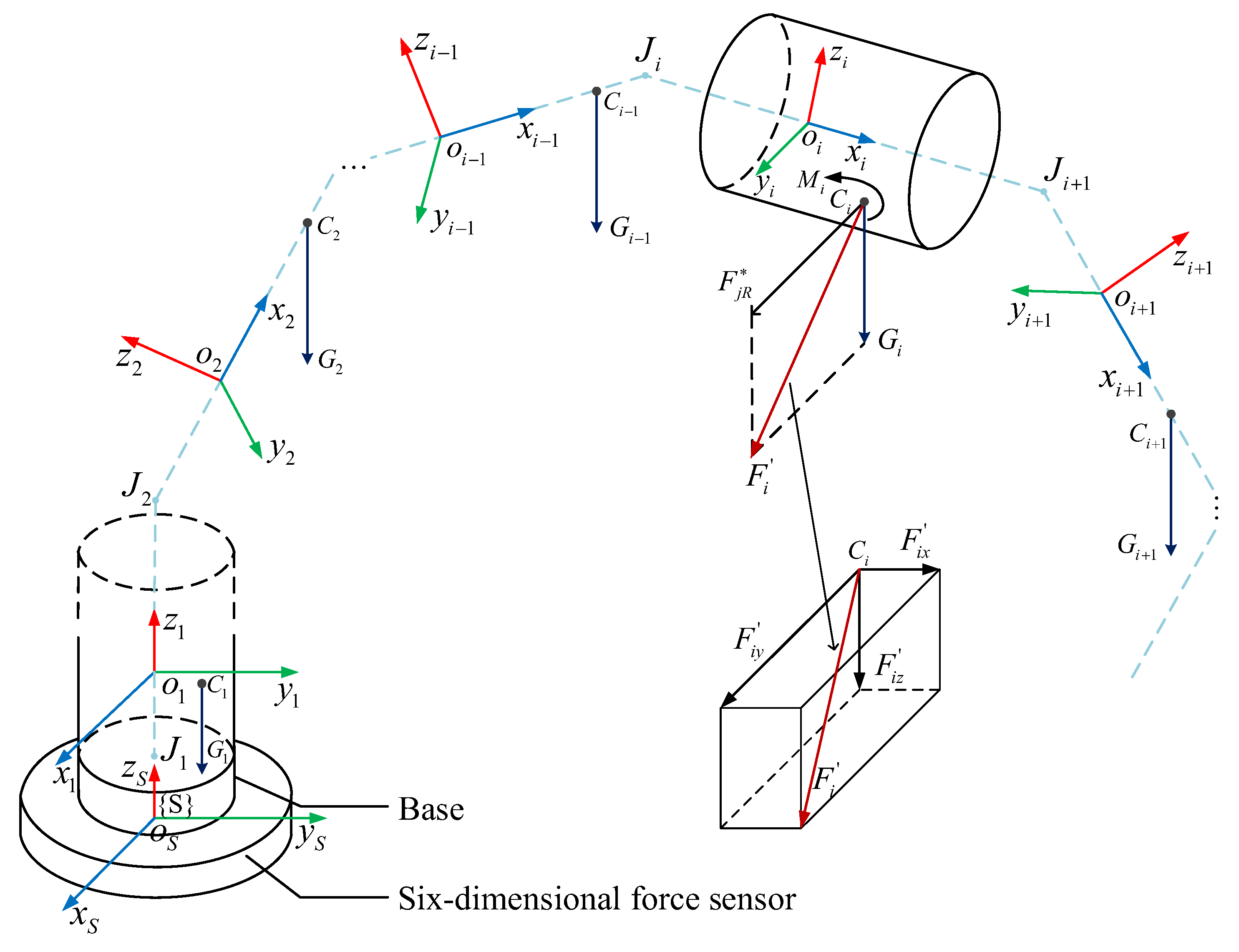
2.1. Collision Detection Model
2.2. Force Compensation Algorithm
2.3. Collision Detection Algorithm
2.4. Solving Examples
- The situation of
- 2.
- The situation of
- 3.
- The situation of
3. Algorithm Verification
3.1. Verification of Force Compensation Algorithm
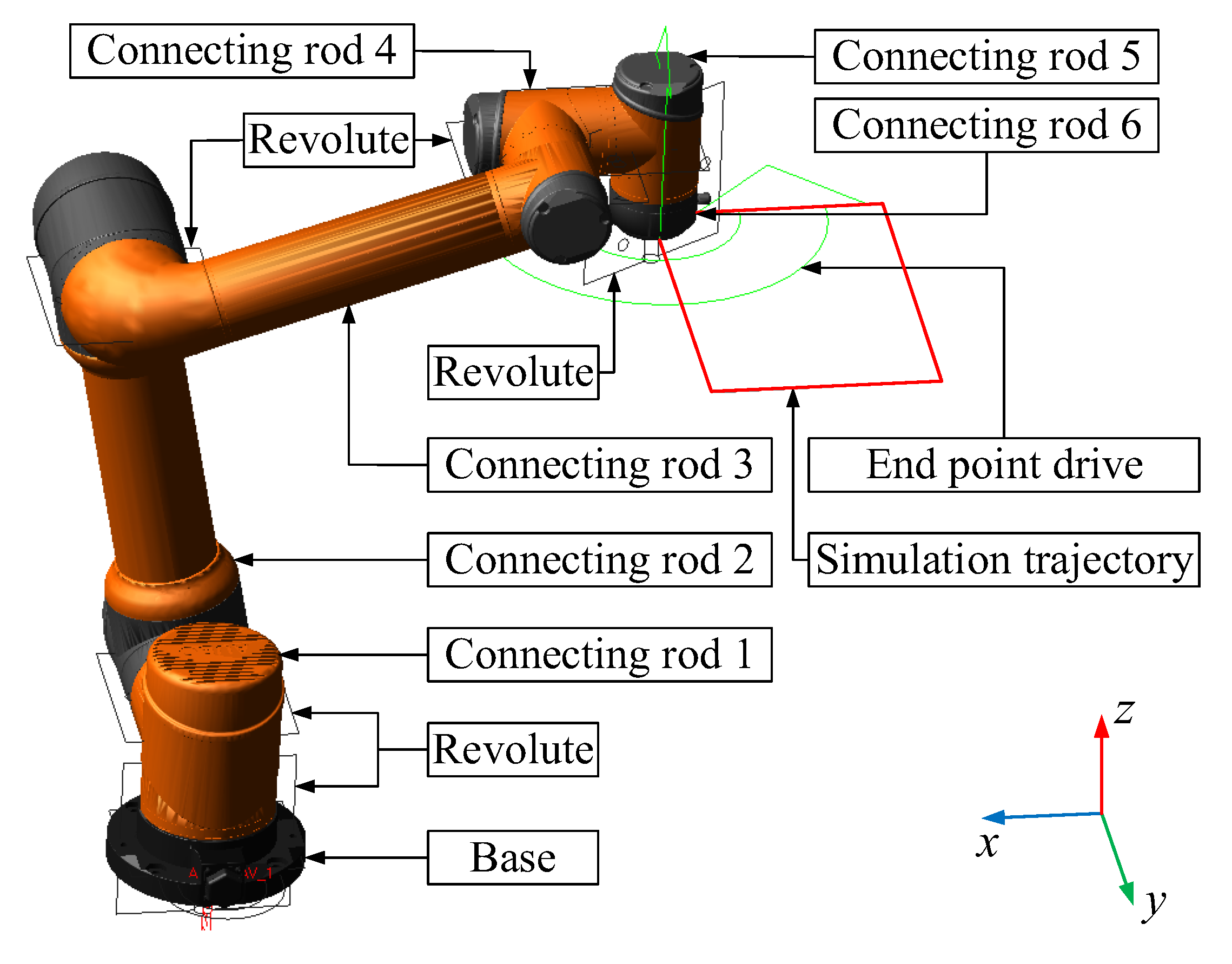
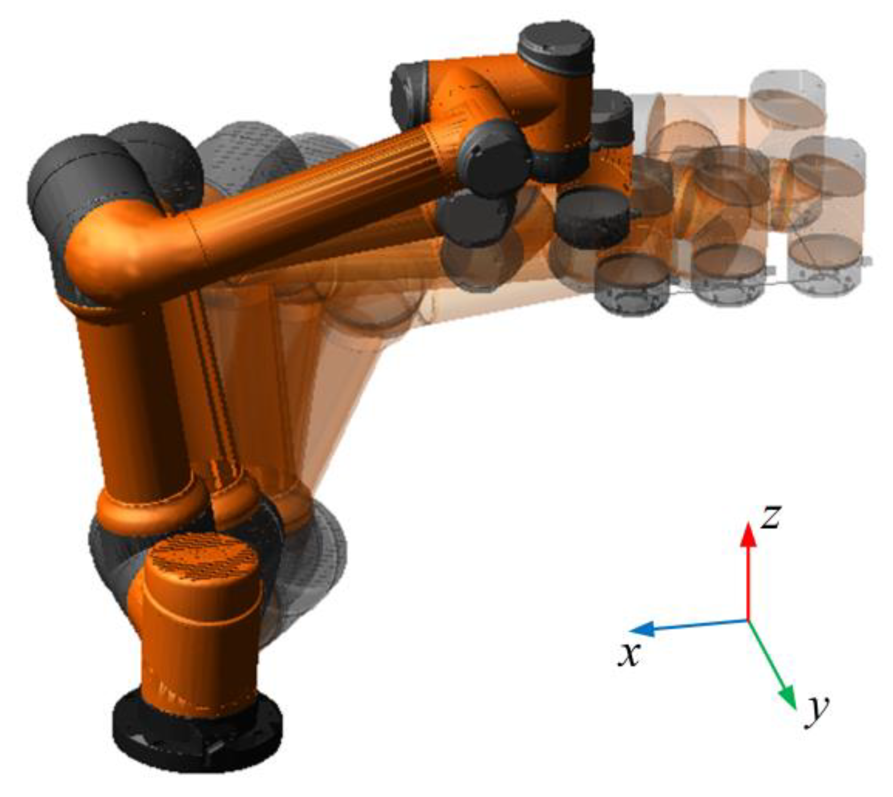
3.1.1. Simulation Verification
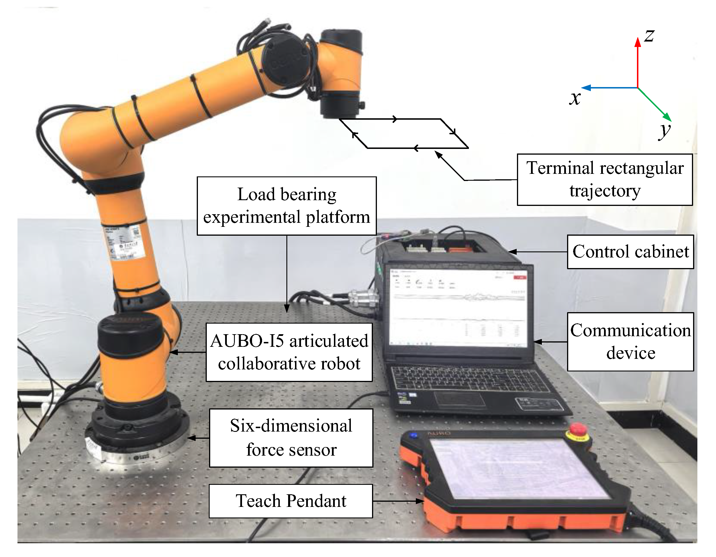
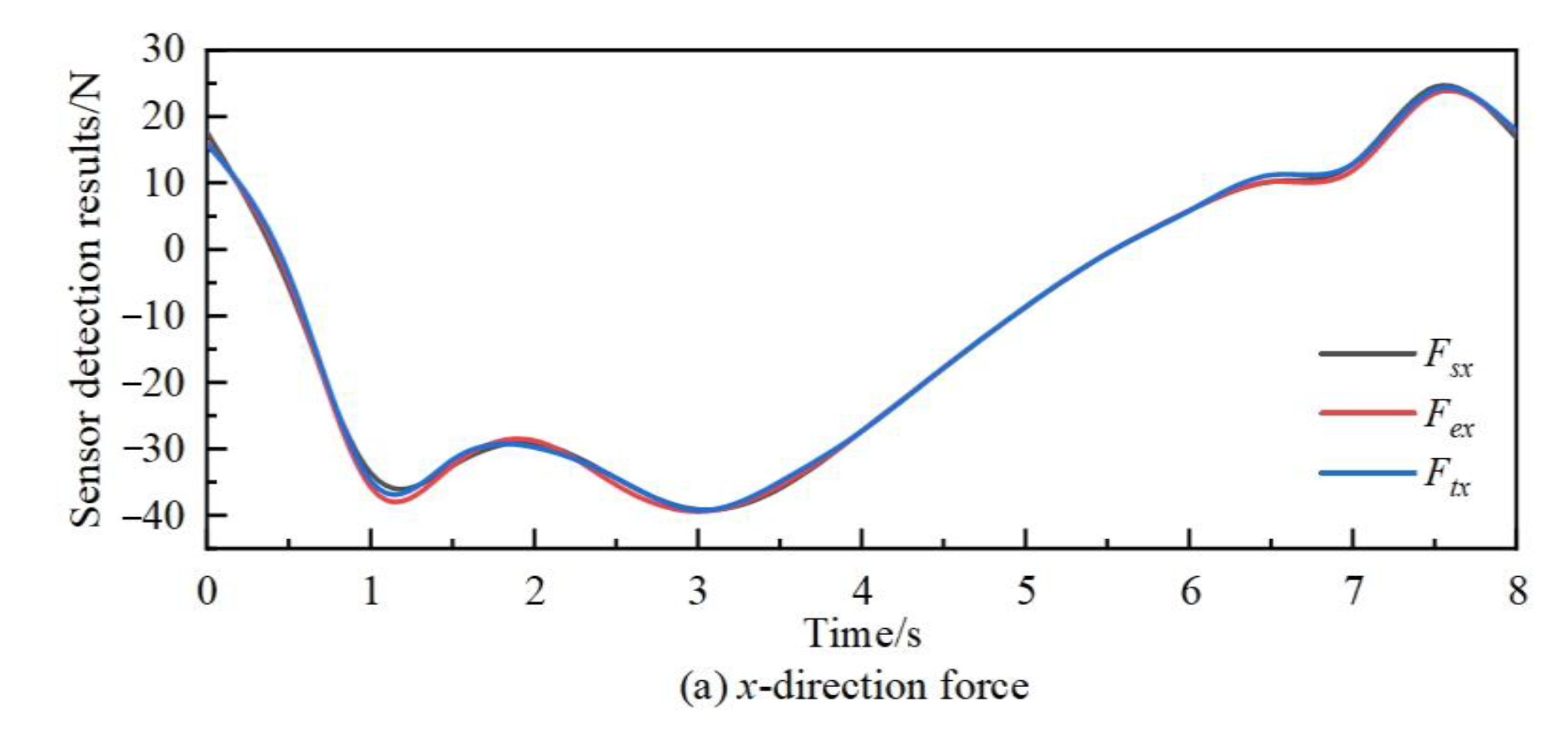
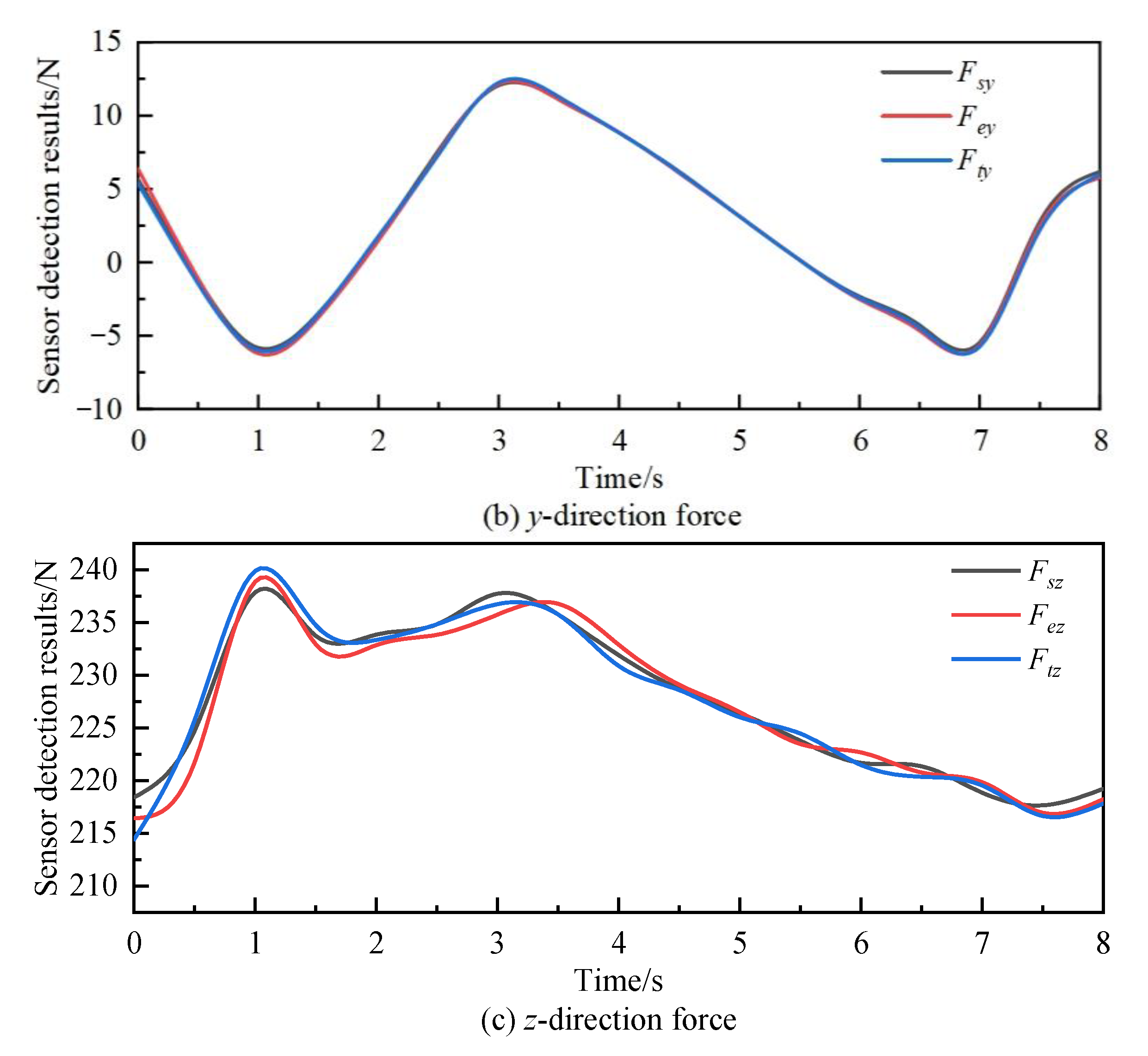
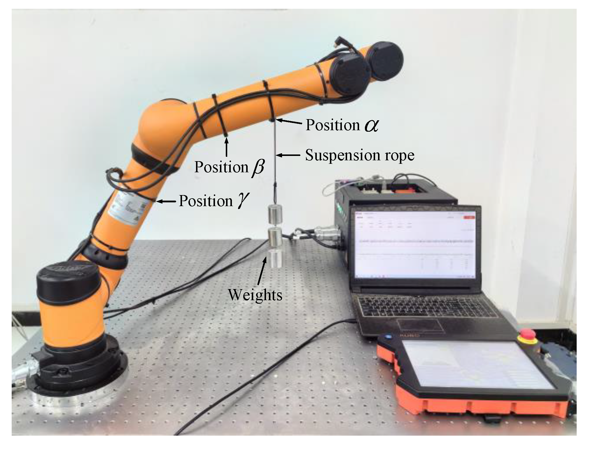
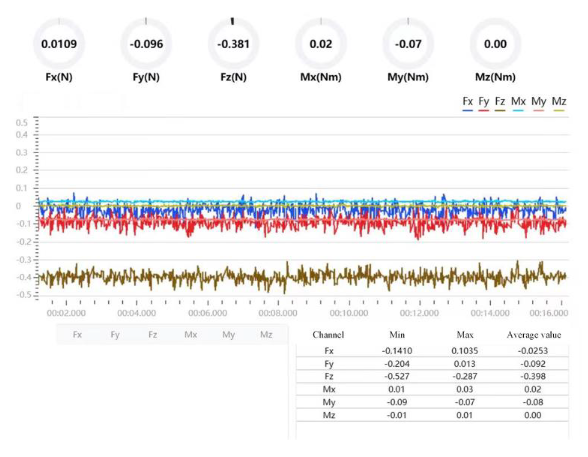
3.1.2. Experimental Verification
3.1.3. Comparative Verification
3.2. Verification of Collision Detection Algorithm
4. Conclusions
Author Contributions
Funding
Data Availability Statement
Conflicts of Interest
References
- Zafar, H.M.; Langås, F.E.; Sanfilippo, F. Exploring the synergies between collaborative robotics, digital twins, augmentation, and industry 5.0 for smart manufacturing: A state-of-the-art review. Robot. Comput. Integr. Manuf. 2024, 89, 102769. [Google Scholar] [CrossRef]
- Dimitropoulos, N.; Michalos, G.; Arkouli, Z.; Kokotinis, G.; Makris, S. Industrial collaborative environments integrating AI, Big Data and Robotics for smart manufacturing. Procedia CIRP 2024, 128, 858–863. [Google Scholar] [CrossRef]
- Singh, A.B.; Himanshu, P. Collaborative robots for industrial tasks: A review. Mater. Today Proc. 2022, 52, 500–504. [Google Scholar] [CrossRef]
- Montini, E.; Cutrona, V.; Dell’Oca, S.; Landolfi, G.; Bettoni, A.; Rocco, P.; Carpanzano, E. A Framework for Human-aware Collaborative Robotics Systems Development. Procedia CIRP 2023, 120, 1083–1088. [Google Scholar] [CrossRef]
- Salgado, K.K.; Dimitropoulos, N.; Michalos, G.; Makris, S. Suitability assessment method for safe robot tooling design in Human-Robot Collaborative applications. Procedia CIRP 2024, 128, 770–775. [Google Scholar] [CrossRef]
- Wang, S.L.; Zhang, J.Q.; Wang, P.; Law, J.; Calinescu, R.; Mihaylova, L. A deep learning-enhanced Digital Twin framework for improving safety and reliability in human–robot collaborative manufacturing. Robot. Comput. Integr. Manuf. 2024, 85, 102608. [Google Scholar] [CrossRef]
- Luca, C.; Emmanuel, F. A Safety 4.0 Approach for Collaborative Robotics in the Factories of the Future. Procedia Comput. Sci. 2023, 217, 1784–1793. [Google Scholar] [CrossRef]
- Park, J.M.; Kim, T.; Gu, C.Y.; Kang, Y.; Cheong, J. Dynamic collision estimator for collaborative robots: A dynamic Bayesian network with Markov model for highly reliable collision detection. Robot. Comput. Integr. Manuf. 2024, 86, 102. [Google Scholar] [CrossRef]
- Wu, Y.; Jia, X.H.; Li, T.J.; Liu, J.Y. A real-time collision avoidance method for redundant dual-arm robots in an open operational environment. Robot. Comput. Integr. Manuf. 2025, 92, 102. [Google Scholar] [CrossRef]
- Xu, X.M.; Gan, Y.H.; Xu, C.; Dai, X.Z. Robot Collision Detection Based on Dynamic Model. In Proceedings of the 2017 Chinese Automation Congress (CAC), Jinan, China, 20–22 October 2017; IEEE: Piscataway, NJ, USA, 2017; pp. 6578–6582. [Google Scholar] [CrossRef]
- Li, W.; Han, Y.; Wu, J.; Xiong, Z.H. Collision Detection of Robots Based on a Force/Torque Sensor at the Bedplate. IEEE ASME Trans. Mechatron. 2020, 25, 2565–2573. [Google Scholar] [CrossRef]
- Svarny, P.; Rozlivek, J.; Rustler, L.; Sramek, M.; Deli, O.; Zillich, M.; Hoffmann, M. Effect of active and passive protective soft skins on collision forces in human–robot collaboration. Robot. Comput. Integr. Manuf. 2022, 78, 102363. [Google Scholar] [CrossRef]
- Xu, T.; Tuo, H.; Fang, Q.Q.; Shan, D.B.; Jin, H.Z.; Fan, J.Z.; Zhu, Y.H.; Zhao, J. A novel collision detection method based on current residuals for robots without joint torque sensors: A case study on UR10 robot. Robot. Comput. Integr. Manuf. 2024, 89, 102777. [Google Scholar] [CrossRef]
- Lv, H.; Liu, L.Y.; Gao, Y.M.; Zhao, S.; Yang, P.P.; Mu, Z.G. A compound planning algorithm considering both collision detection and obstacle avoidance for intelligent demolition robots. Rob. Auton. Syst. 2024, 181, 104781. [Google Scholar] [CrossRef]
- Mu, Z.G.; Liu, L.Y.; Jia, L.H.; Zhang, L.Y.; Ding, N.; Wang, C.J. Intelligent demolition robot: Structural statics, collision detection, and dynamic control. Autom. Constr. 2022, 142, 104490. [Google Scholar] [CrossRef]
- Sun, T.; Sun, J.R.; Lian, B.B.; Li, Q. Sensorless admittance control of 6-DoF parallel robot in human-robot collaborative assembly. Robot. Comput. Integr. Manuf. 2024, 88, 102742. [Google Scholar] [CrossRef]
- Li, Z.J.; Ye, J.H.; Wu, H.B. A Virtual Sensor for Collision Detection and Distinction with Conventional Industrial Robots. Sensors 2019, 19, 2368. [Google Scholar] [CrossRef]
- Zhou, C.B.; Xia, M.Y.; Xu, Z.B. A six dimensional dynamic force/moment measurement platform based on matrix sensors designed for large equipment. Sens. Actuators A Phys. 2023, 349, 114085. [Google Scholar] [CrossRef]
- He, Z.X.; Liu, T. Design of a three-dimensional capacitor-based six-axis force sensor for human-robot interaction. Sens. Actuators A Phys. 2021, 331, 112939. [Google Scholar] [CrossRef]
- Zhang, Z.J.; Chen, Y.P.; Zhang, D.L.; Xie, J.M.; Liu, M.Y. A six-dimensional traction force sensor used for human-robot collaboration. Mechatronics 2019, 57, 164–172. [Google Scholar] [CrossRef]
- Li, Y.J.; Wang, G.C.; Zhang, J.; Jia, Z.Y. Dynamic characteristics of piezoelectric six-dimensional heavy force/moment sensor for large-load robotic manipulator. Measurement 2012, 45, 1114–1125. [Google Scholar] [CrossRef]
- Pu, M.H.; Luo, C.X.; Wang, Y.Z.; Yang, K.Y.; Zhao, R.D.; Tian, L.X. A configuration design approach to the capacitive six-axis force/torque sensor utilizing the compliant parallel mechanism. Measurement 2024, 237, 115205. [Google Scholar] [CrossRef]
- Sun, Y.J.; Liu, Y.W.; Zou, T.; Jing, M.H.; Liu, H. Design and optimization of a novel six-axis force/torque sensor for space robot. Measurement 2015, 65, 135–148. [Google Scholar] [CrossRef]
- Li, Y.J.; Sun, B.Y.; Zhang, J.; Qian, M.; Jia, Z.Y. A novel parallel piezoelectric six-axis heavy force/torque sensor. Measurement 2008, 42, 730–736. [Google Scholar] [CrossRef]
- Chen, D.F.; Song, A.G.; Li, A. Design and Calibration of a Six-axis Force/torque Sensor with Large Measurement Range Used for the Space Manipulator. Procedia Eng. 2015, 99, 1164–1170. [Google Scholar] [CrossRef]
- Wang, Z.J.; Li, Z.X.; He, J.; Yao, J.T.; Zhao, Y.S. Optimal design and experiment research of a fully pre-stressed six-axis force/torque sensor. Measurement 2013, 46, 2013–2021. [Google Scholar] [CrossRef]
- Templeman, J.O.; Sheil, B.B.; Sun, T. Multi-axis force sensors: A state-of-the-art review. Sens. Actuators A Phys. 2020, 304, 111772. [Google Scholar] [CrossRef]
- Cai, D.J.; Yao, J.T.; Gao, W.H.; Zhang, H.Y.; Li, Z.Y. Design and analysis of parallel six-dimensional force sensor based on near-singular characteristics. Meas. Sci. Technol. 2024, 35, 045116. [Google Scholar] [CrossRef]
- Park, J.Y.; Lee, J.Y.; Kim, S.H.; Kim, S.R. Optimal Design of Passive Gravity Compensation System for Articulated Robots. Trans. Korean Soc. Mech. Eng. A 2012, 36, 103–108. [Google Scholar] [CrossRef]
- Duan, J.J.; Liu, Z.C.; Bin, Y.M.; Cui, K.K.; Dai, Z.D. Payload Identification and Gravity/Inertial Compensation for Six-Dimensional Force/Torque Sensor with a Fast and Robust Trajectory Design Approach. Sensors 2022, 22, 439. [Google Scholar] [CrossRef]
- Wang, Z.J.; Lu, L.; Yan, W.K.; He, J.; Cui, B.Y.; Li, Z.X. Research on Collision Point Identification Based on Six-Axis Force/Torque Sensor. J. Sens. 2020, 2020, 881263. [Google Scholar] [CrossRef]
- Konstantinos, K.; Haninger, K.; Gkrizis, C.; Dimitropoulos, N.; Kruger, J.; Michalos, G.; Makris, S. Collision detection for collaborative assembly operations on high-payload robots. Robot. Comput. Integr. Manuf. 2024, 87, 102708. [Google Scholar] [CrossRef]
- Shi, W.; Xi, A.M.; Zhang, Y.B. Robot Dynamics Modeling and Simulation Based on Kane. Microcomput. Inf. 2008, 29, 222–223. (In Chinese) [Google Scholar]
- Chen, Z.G.; Ruan, X.G.; Li, Y. Dynamic Modeling of a Self-balancing Cubical Robot. J. Beijing Univ. Technol. 2018, 44, 376–381. (In Chinese) [Google Scholar]
- Zuo, B.; Liu, J.G.; Li, Y.M. Dynamic Modeling on the Parallel Active Vibration Isolation System of Space Station Science Experimental Rack. Mach. Des. Manuf. 2014, 3, 199–203. (In Chinese) [Google Scholar]


| Modeling Method | Number of Operations | |
|---|---|---|
| Multiplication | Addition | |
| Lagrange method | 2195 | 1719 |
| Newton–Euler method | 1541 | 1196 |
| Kane method | 646 | 394 |
| Number | Value Situation | The Range of Values for x | Number of Collision Points | Collision Point Coordinates | Sketch Map |
|---|---|---|---|---|---|
| 1 | none | 0 | none |  | |
| 2 | 0 | none | 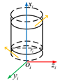 | ||
| 3 | 1 | 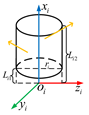 | |||
| 4 | or | 0 | none | 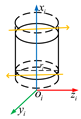 | |
| 5 | or | 1 | 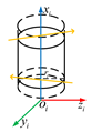 | ||
| 6 | or | 2 | or | 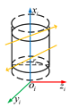 | |
| 7 | 2 | 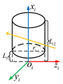 | |||
| 8 | 2 | 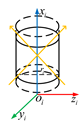 | |||
| 9 | 2 | 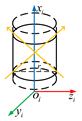 |
| Condition | Function |
|---|---|
| x-direction translation | Step (time, 0, 0, 1, −200) + step (time, 3, 0, 7, 200) |
| y-direction translation | Step (time, 1, 0, 3, 300) + step (time, 7, 0, 8, −300) |
| z-direction translation | 0 * time |
| Rotate around the x-axis direction | 0 * time |
| Rotate around the y-axis direction | 0 * time |
| Rotate around the z-axis direction | 0 * time |
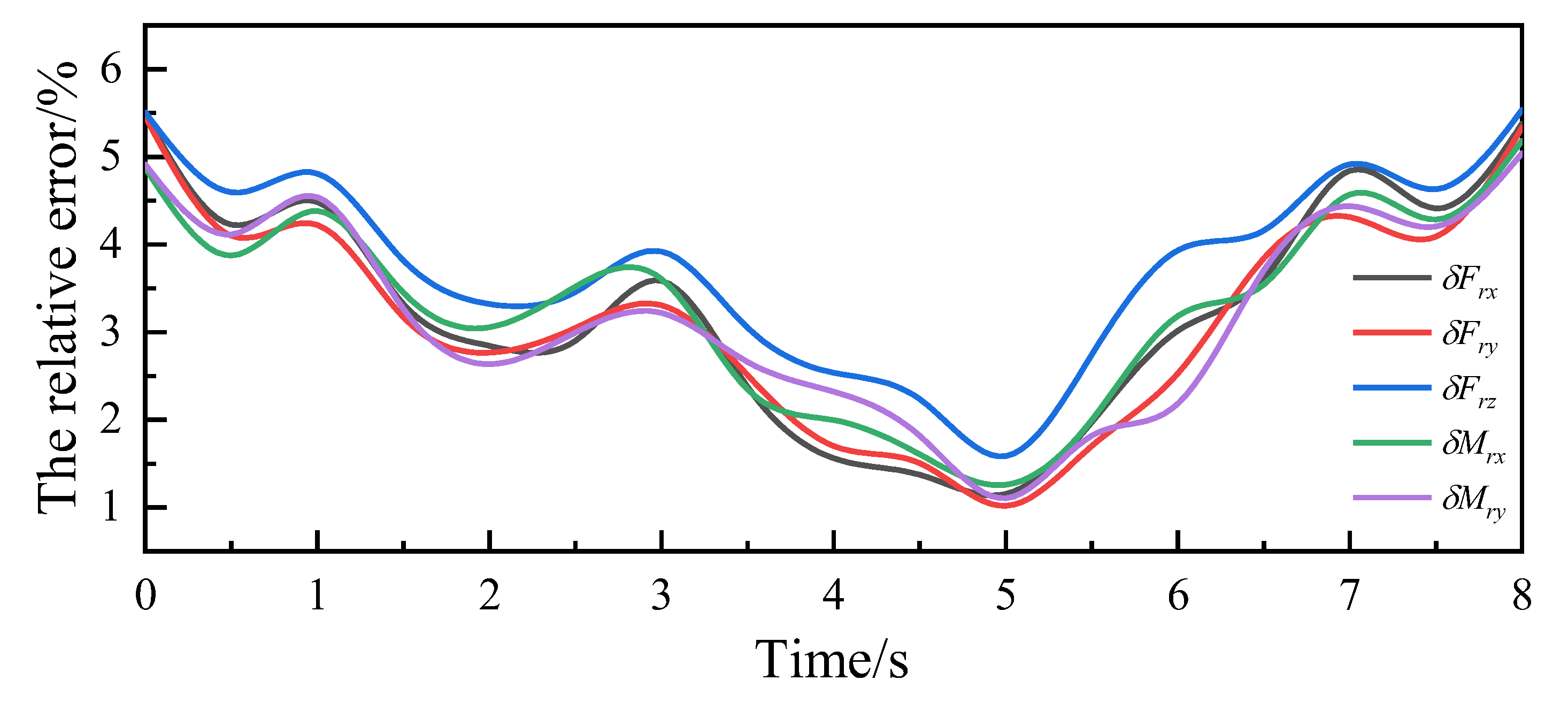
| Relative Error | /% | /% | /% | /% | /% |
|---|---|---|---|---|---|
| Value | 5.4824 | 5.4602 | 5.5359 | 5.1854 | 5.0423 |
| Collision Position | x-Direction Vector/mm | y-Direction Vector/mm | z-Direction Vector/mm |
|---|---|---|---|
| α | −14.10 | −35.54 | 51.36 |
| β | −13.93 | −25.61 | 48.17 |
| γ | −8.45 | −16.52 | 33.15 |
| Number | Collision Force/N | Three Directional Force Vectors/N | Three Directional Torque Vectors/(N·mm) | Calculate Position/mm | Absolute Position Error/mm | Relative Positional Error/% |
|---|---|---|---|---|---|---|
| 1 | 5.88 | −0.2529 | −0.0027 | −12.5749 | 1.5251 | 5.7923 |
| −0.1854 | 0.0931 | −34.0196 | 1.5204 | |||
| 0.5435 | −0.0287 | 50.6327 | 0.7273 | |||
| 2 | 7.84 | −0.2688 | −0.0900 | −12.6538 | 1.4462 | 5.0752 |
| −0.1807 | 0.2432 | −34.5375 | 1.0025 | |||
| 0.7253 | −0.0247 | 50.5591 | 0.8009 | |||
| 3 | 9.80 | −0.2195 | −0.0127 | −15.1268 | 1.0268 | 3.8751 |
| −0.0523 | 0.0969 | −36.2093 | 0.6693 | |||
| 0.8790 | −0.0256 | 50.5749 | 0.7851 | |||
| 4 | 11.76 | −0.3560 | −0.0045 | −13.4817 | 0.6183 | 2.5957 |
| −0.2608 | 0.1274 | −35.0753 | 0.4647 | |||
| 1.0016 | −0.0479 | 50.7810 | 0.5790 |
Disclaimer/Publisher’s Note: The statements, opinions and data contained in all publications are solely those of the individual author(s) and contributor(s) and not of MDPI and/or the editor(s). MDPI and/or the editor(s) disclaim responsibility for any injury to people or property resulting from any ideas, methods, instructions or products referred to in the content. |
© 2025 by the authors. Licensee MDPI, Basel, Switzerland. This article is an open access article distributed under the terms and conditions of the Creative Commons Attribution (CC BY) license (https://creativecommons.org/licenses/by/4.0/).
Share and Cite
Wang, Y.; Wang, Z.; Feng, Y.; Xu, Y. Research on Robot Force Compensation and Collision Detection Based on Six-Dimensional Force Sensor. Machines 2025, 13, 544. https://doi.org/10.3390/machines13070544
Wang Y, Wang Z, Feng Y, Xu Y. Research on Robot Force Compensation and Collision Detection Based on Six-Dimensional Force Sensor. Machines. 2025; 13(7):544. https://doi.org/10.3390/machines13070544
Chicago/Turabian StyleWang, Yunyi, Zhijun Wang, Yongli Feng, and Yanghuan Xu. 2025. "Research on Robot Force Compensation and Collision Detection Based on Six-Dimensional Force Sensor" Machines 13, no. 7: 544. https://doi.org/10.3390/machines13070544
APA StyleWang, Y., Wang, Z., Feng, Y., & Xu, Y. (2025). Research on Robot Force Compensation and Collision Detection Based on Six-Dimensional Force Sensor. Machines, 13(7), 544. https://doi.org/10.3390/machines13070544