Temperature Analysis of Secondary Plate of Linear Induction Motor on Maglev Train Under Periodic Running Condition and Its Optimization

Abstract

The propulsion system is a critical component of medium–low-speed maglev trains and the single-sided linear induction motor (SLIM) has been adopted to generate thrust. However, the SLIM operates periodically in maglev trains. The temperature of the secondary plate of the SLIM rises significantly due to eddy currents when the train enters and leaves the station, where large slip occurs. Subsequently, the temperature decreases through natural cooling during the shift interval time. This periodic operating condition is rarely addressed in the existing literature and warrants attention, as the temperature accumulates over successive periods, potentially resulting in thermal damage and thrust variation. Furthermore, the conductivity of plate varies significantly in the process, which affects the losses and thrust, requiring a coupled analysis. To investigate the temperature variation patterns, this paper proposes a coupled model integrating the lumped parameter thermal network (LPTN) and the equivalent circuit (EC) of the SLIM. Given the unique structure of the F-shaped rail, the LPTN mesh is well designed to account for the skin effect. Three experiments and a finite element method (FEM)-based analysis were conducted to validate the proposed model. Finally, optimizations were performed with respect to different shift interval time, plate materials, and carriage numbers. The impact of temperature on thrust is also discussed. The results indicate that the minimum shift interval time and maximum carriage number are 70.7 s and 9, respectively, with thrust increasing by 22.0% and 22.0%. Furthermore, the use of copper as the plate material can reduce the maximum temperature by 22.01% while decreasing propulsion thrust by 26.1%.

1. Introduction

The widespread adoption of maglev trains since the late 20th century has significantly enhanced urban mobility due to their eco-friendly operation, minimal noise emissions, and high-speed capabilities. medium–low-speed maglev systems, operating within the 70–130 km/h range, are particularly well suited for urban transit applications [1]. LIMINO from Japan and ECOBEE from Korea started their commercial running at a speed of 110km/h in 2005 and 2016 [2]. In China, the Beijing S1 line and Changsha maglev also received attention, connecting transportation hubs like airports with the city center [3].

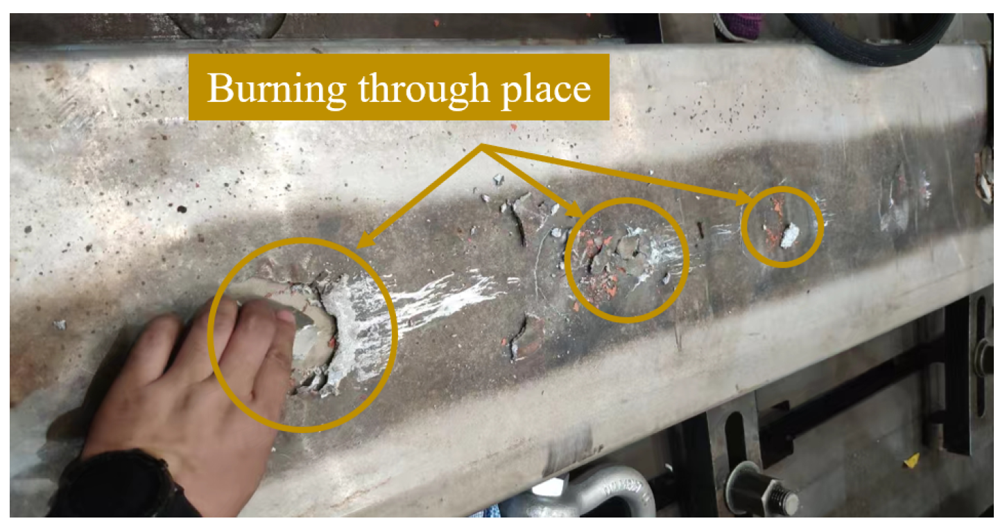
Single-sided linear induction motors (SLIMs) are widely adopted as a propulsion system for medium–low-speed maglev trains due to their cost-effectiveness, high thrust capability, and control simplicity. However, eddy currents induced in the conductive plate generate a substantial temperature rise, a critical consideration particularly under high-slip operating conditions, such as during the entering and leaving (E&L) station stage. While in the passenger waiting (W) stage, the time of which is also known as the shift interval time, the plate temperature drops by natural cooling. The translational motion of the train causes the SLIM to operate under periodic thermal loading. This cyclic operation leads to a cumulative temperature rise in the secondary conductive plate, inducing material thermal fatigue and, in severe cases, thermal breakdown due to excessive heating. In laboratory tests, a burn-through of the secondary plate has been observed, as demonstrated in Figure 1.

As a result, a thorough thermal research about the secondary plates of SLIMs is necessary to prevent heat accidents during maglev train operations.

Numerous studies have been conducted on the thermal field analysis of induction motors. A lumped parameter thermal network (LPTN) is widely used. Ref. [4] proposed a thermal equivalent network and applied it to a 5.5 MW shielding induction motor, which is used in the cooling system of a nuclear power plant. The proposed methodology explicitly incorporates the actual transposition geometry of stator strands and its consequential effects on heat generation distribution, enabling high-fidelity thermal field modeling. To eliminate the effects caused by changing thermal parameters, a virtual sensing strategy incorporating an LPTN is proposed in [5] to realize a more efficient method. In [6], the temperature of each part of the induction motor is obtained by an LPTN, and then a lifespan estimation is conducted and verified in an experiment. In [7], Joule and iron losses are used as the input of an LPTN, and the temperature result is validated by MATLAN software. By introducing a cooling system into an LPTN, ref. [8] broadened the scope of the motor design, and then a 13 kW induction motor was tested to validate the LPTN.

Besides the LPTN, the finite element method (FEM) is also frequently adopted. Ref. [9] conducted a simulation for a 15 kW totally enclosed fan cooled (TEFC) induction motor to safely run an electric vehicle. A two-dimensional transient FEM is established in [10] to analyze the performance and temperature of an induction motor under different heat exchange rates. Fins are added over the induction motor to reach larger heat dissipation areas in [11], where two different FEMs, ANSYS (https://www.ansys.com/) and Motor-CAD (https://www.ansys.com/products/electronics/ansys-motor-cad), are both used to evaluate the temperature of this unique structure. Ref. [12] conducted a simulation of an induction motor with water-cooling, non-ventilated and polymer-encapsulated stator windings. It is concluded that over 60% reduction in temperature is reached by the water. Aiming at unbalanced supply voltages and inter-turn short-circuit condition occasions, ref. [13] established faulty scenarios via an FEM, under which the thermal situation of the motor is researched.

Furthermore, the temperature can be obtained by the resistance of secondary plates. Ref. [14] calculated the temperature of a rotor based on metal resistance. To speed up convergence, the method extracts rotor slot harmonics from stator current for real-time speed detection and uses the first 5–15 startup cycles to simulate locked-rotor conditions, obtaining more accurate initial leakage inductance and resistances. In [15], the formula of the rotor resistance, the temperature of the stator, and the rotor windings are synthesized by adopting a rotating two-phase coordinate system. Then, a new method calculating the rotor temperature by resistance is proposed and validated by MATLAB (https://matlab.mathworks.com/). Due to the larger thermal inertia of the motor shell, a set of modules is developed in [16] to evaluate the temperature in a more precise way.

With the growth of artificial intelligence, deep learning is also used in the temperature calculation. An automatic method for detecting the faults in induction motors is proposed based on thermal images in [17]. Furthermore, ref. [18] realized functions of not only temperature identification, but also of detecting broken rotor coils, shortening stator coils and other abnormal situations.

Coupled analysis plays an important role in thermal research as during the process, the conductivity of the plate varies considerably. Ref. [19] obtains the losses by conducting an FEM of an electromagnetic field. Then, the loss value is introduced into the LPTN to calculate the temperature. To avoid the previous FEM’s limitations, ref. [20] proposes a new method that minimizes the use of FEM. The authors first perform the FEM to obtain important factors in an equivalent circuit (EC) of the induction motor. After that, a model that combines EC with LPTN is proposed. Ref. [21] uses a weak coupled modeling technique, and the effect of the air gap is also discussed. Based on modern design packages, ref. [22] developed a comprehensive software, where an induction motor is used to validate the correctness. Ref. [23] investigates a 3D FEM to calculate Joule losses, which are then included in the thermal equations. An equivalent cooling condition when the rotor is working is discussed.

In addition, the thermal field for a linear induction motor is seldom discussed in the existing literature. Although there are several [24,25,26], their primary focus, however, is the electromagnetic launcher system, which operates at high voltage and large current capacities with a fundamentally different configuration from maglev SLIMs. Its secondary conductive structure comprises both a plate and rail assembly, where the rail region exhibits significant skin effects due to vertical flux density gradients. Furthermore, current thermal–electromagnetic coupling models remain incomplete, still relying on FEM implementations. Crucially, the existing literature [27,28,29] fails to address the periodic operational regime of SLIMs, necessitating further investigation into their characteristic temperature fluctuation patterns and associated thermal failure mechanisms.

As a result, to establish a pure analytical thermal–electromagnetic mutually coupled model, a prototype of SLIM is manufactured in Section 2. An EC of the SLIM is proposed considering end and edge effects to calculate the secondary loss in Section 3. A 2D LPTN is established in Section 4 to model the transfer path of the heat flow as the method to obtain the thermal field. The mesh of the LPTN is well designed in the secondary part to account for the skin effect. Then, the coupled model is established to analyze the temperature variation of the plate. In Section 5, experiments including periodic running conditions and simulations are both carried out. After verifying the correctness of the model, optimizations of magelv train details, including shift interval time, plate material and carriage number, are conducted and presented in Section 6. Furthermore, the thrust variation due to the temperature is discussed in this part.

Based on the model, the optimal shift interval time and carriage number are obtained as 70.7 s and 9. By replacing the aluminum plate with a cooper plate, the maximum temperature drops by 22.01%. This study proposes an enhanced methodology for secondary temperature computation and offers optimized selection criteria for maglev operational parameters, including shift interval time, carriage number and plate material.

2. Prototype SLIM Structure

Figure 2 shows the structure of a naturally cooled 4-pole and 72-slot SLIM adopted in the experiment, which is also used in medium–low-speed maglev trains for propulsion.

The SLIM consists of two components: the primary and the secondary. The primary core utilizes laminated iron to minimize eddy current losses, while the windings employ aluminum conductors for weight reduction. During operation, balanced three-phase currents in the primary windings establish a traveling magnetic field across the air gap. This field induces eddy currents in the secondary conductive plate, generating propulsion force. The F-shaped back iron rail serves the purposes of magnetic flux guidance to improve the performance. Key operational parameters and material thermal properties are detailed in

Table 1. Rated parameters of SLIM prototype.

Symbol	Description	Value	Unit
d	Thickness of plate	4	mm
$\delta$	Air-gap length	13	mm
${\sigma }_{plate}$	Conductivity of the plate	3.1 × 107	S/m
$\tau$	Pole pitch	225	mm
${\tau }_{cp}$	Coil pitch	8/9
p	Pole pair	4
$b_t$	Teeth width	7.9	mm
$b_s$	Slot width	14.6	mm
a	Width of half core	110	mm
c	Width of half plate	121	mm
m	Phase number	3
n	Slot number	72
L	Primary length	1807.9	mm
I	Primary current	350	A
f	Frequency	13.69	Hz
${\lambda }_{Rail}$	Rail thermal conductivity	78	W/(mK)
${\lambda }_{plate}$	Plate thermal conductivity	238	W/(mK)
${\lambda }_c$	Air thermal conductivity	0.026	W/(mK)
$T_0$	Ambient temperature	25.0	°C

.

3. EC Model Establishment

Figure 3 proposes an EC model for the SLIM to quantify secondary losses, which directly influence the temperature distribution in the conductive secondary plate. The open-ended topology of SLIM necessitates explicit consideration of both longitudinal end effects and transverse edge effects in magnetic field computations, as these phenomena significantly impact loss determination accuracy. These effects are considered in the proposed EC by introducing four coefficients, $C_x$, $C_r$, $K_x$ and $K_r$, to correct the secondary resistance and magnetizing inductance [30,31].

The EC consists of primary resistance $R_1$, primary leakage inductance $L_1$, magnetizing inductance $L_m$ and secondary resistance $R_2$. Secondary leakage inductance $L_2$ and magnetizing resistance $R_m$ are both neglected due to their small values, as determined by the manufacturing design. $R_2$ is composed of $R_{plate}$ and $R_{rail}$ in parallel, which is, respectively, the equivalent resistance of the secondary reaction plate and the resistance of the F-shaped rail.

3.1. Equivalent Circuit Parameter Calculation

$R_1$ is the primary resistance that is equal to the resistance of primary winding per phase. It is calculated by

$$R_1={\rho }_{Coil}{\displaystyle \frac{L_{Coil}}{A_{Coil}}}$$

(1)

where ${\rho }_{Coil}$, $L_{Coil}$ and $A_{Coil}$ are, respectively, the resistivity, length and sectional area of the coil.

${\rho }_{Coil}$ is indeed related to temperature, but the temperature variation is not significant enough in the winding part to cause a considerable change in resistance. Furthermore, it is the current source instead of the voltage source that is used. The change in ${\rho }_{Coil}$ does not affect the final excitation. As a result, the temperature impact on the primary resistance is neglected in this article.

Magnetizing inductance is defined as

$$L_m={\displaystyle \frac{2{\mu }_0\tau ·2a·{\left(N_s·k_{dp}\right)}^2}{{\pi }^2{p}_e{\delta }_e}}$$

(2)

where ${\mu }_0$ is the vacuum permeability, a is half the width of the primary, $\tau$ is the pole pitch, $N_s$ is the number of winding in one series, $k_{dp}$ is the winding coefficient and $p_e$ is the equivalent pole pair, which is obtained by [30]

$$p_e={\displaystyle \frac{{\left(2p-1\right)}^2}{4p-3+\epsilon /\phantom{\epsilon \left(mq\right)}\left(mq\right)}}$$

(3)

where p is the pole pair, q is the slot number per pole per phase, $\epsilon$ is the shorten pitch and m is the phase number.

${\delta }_e$ is the equivalent air-gap length, which is calculated by

$${\delta }_e=k_{\delta }{k}_m\left({\delta }_{air}+d_{plate}\right)$$

(4)

In the above, $k_{\delta }$ and $k_m$ [32] are the Carter and magnetic saturation coefficients, respectively; ${\delta }_{air}$ is the length of the air gap and $d_{plate}$ is the thickness of the secondary plate.

The structure of the secondary plate consists of the reaction plate and the back iron, which is the F-shaped rail in a maglev propulsion system. As a result, the secondary resistance $R_2$ is composed of $R_{plate}$ and $R_{rail}$ in parallel, which can be calculated by [30]

$$R_{plate}=4{\rho }_{plate}{\displaystyle \frac{a·{\left(N_s{k}_{dp}\right)}^2}{\tau p_e{d}_{plate}}}$$

(5)

$$R_{rail}=4{\rho }_{rail}{\displaystyle \frac{a·{\left(N_s{k}_{dp}\right)}^2}{\tau p_e{d}_{Fe}}}$$

(6)

$$R_2={\displaystyle \frac{R_{rail}{R}_{plate}}{R_{rail}+R_{plate}}}$$

(7)

where ${\rho }_{plate}$ and ${\rho }_{rail}$ are the resistivity of the material of the plate and rail. They are also related to temperature. $d_{Fe}$ is the equivalent depth of the F-shaped rail affected by the skin effect, which can be obtained by

$$d_{Fe}=\sqrt{{\displaystyle \frac{{\rho }_{rail}}{\pi f{\mu }_0{\mu }_{rail}}}}$$

(8)

where f is the frequency of the source and ${\mu }_{rail}$ is the relative permeability of the material of the rail, whereby iron is selected as the rail material in this article.

3.2. Edge and End Effect Coefficient Calculation

The edge and end effects are caused by the structural asymmetry and moving characteristic of the SLIM, which negatively impact its performance. In order to compensate for the error, four coefficients are introduced in the EC, which are calculated below:

$$K_r={\displaystyle \frac{s{G}_{SLIM}}{2p_e\tau \sqrt{1+{\left(s{G}_{SLIM}\right)}^2}}}{\displaystyle \frac{C_1^2+C_2^2}{C_1}}$$

(9)

$$K_x={\displaystyle \frac{1}{2p_e\tau \sqrt{1+{\left(s{G}_{SLIM}\right)}^2}}}{\displaystyle \frac{C_1^2+C_2^2}{C_2}}$$

(10)

$$C_r={\displaystyle \frac{s{G}_{SLIM}\left({\mathrm{Re}}^2\left[T_e\right]+{\mathrm{Im}}^2\left[T_e\right]\right)}{\mathrm{Re}\left[T_e\right]}}$$

(11)

$$C_x={\displaystyle \frac{{\mathrm{Re}}^2\left[T_e\right]+{\mathrm{Im}}^2\left[T_e\right]}{\mathrm{Im}\left[T_e\right]}}$$

(12)

where s is the slip of SLIM and $G_{SLIM}$ is the goodness factor of SLIM, which is obtained by

$$G_{SLIM}={\displaystyle \frac{2{\mu }_0{\sigma }_{s}f{\tau }^2}{\pi {\delta }_e}}$$

(13)

where

$${\sigma }_e={\displaystyle \frac{d_{plate}}{{\rho }_{plate}}}$$

(14)

$C_1$, $C_2$ and $T_e$ are the functions of the parameter of SLIM and are calculated in detail in [30,33].

3.3. Output Parameter Calculation

The power related to the element $(1-s)R_2/s$ represents the mechanical energy. As a result, the thrust of SLIM can be calculated by

$$F={\displaystyle \frac{m{I}_2^2{C}_r{K}_r{R}_2}{2\tau sf}}$$

(15)

where m is the number of phases and $I_2$ is the current of the secondary branch and can be obtained by

$$I_2={\displaystyle \frac{2\pi f{C}_x{K}_x{L}_m}{\sqrt{{\left(2\pi f{C}_x{K}_x{L}_m\right)}^2+{\left(C_r{K}_r{R}_2/\phantom{C_r{K}_r{R}_{2}s}s\right)}^2}}}{I}_1$$

(16)

Secondary power losses that consist of the plate loss and back iron loss are the heat source of rising plate temperature. It should be calculated correctly and be introduced into the subsequent thermal network model. In the EC, $R_2$ represents the heat power, so the secondary power loss is obtained by

$$p_2=m{I}_2^2{C}_r{K}_r{R}_2$$

(17)

The loss of the plate and iron are calculated, respectively, by

$$p_{plate}=m{I}_2^2{C}_r{K}_r{R}_2{\displaystyle \frac{R_{rail}}{R_{rail}+R_{plate}}}$$

(18)

$$p_{iron}=m{I}_2^2{C}_r{K}_r{R}_2{\displaystyle \frac{R_{plate}}{R_{rail}+R_{plate}}}$$

(19)

4. Transit Temperature Analysis and Coupled Model

4.1. LPTN Establishment

With regard to the LPTN, the temperature field consists of different nodes. The temperature remains the same in the part presented by the same node. Heat resistance exists between two certain nodes and presents the heat transfer path [34].

It should be mentioned that the low thermal conductivity of air effectively inhibits heat transfer from the high-heating-power secondary to the primary core, resulting in negligible thermal influence on the latter. Therefore, only the temperature distribution of the secondary plate is analyzed, and the corresponding LPTN is established in a later discussion.

As for the LPTN of the secondary plate, firstly, the structure exhibits longitudinal uniformity. Secondly, while eddy currents in the conductive plate propagate longitudinally, their rapid movement relative to thermal time constants allows them to be modeled as stationary heat sources at discrete positions. These sources maintain longitudinal uniformity in both heat generation and distribution. Additionally, the system employs natural convection cooling, whose effectiveness remains consistent along the length of the structure.

As a result, to simplify the LPTN’s complexity and save computation time, a transient 2D LPTN instead of a 3D one is proposed in this section to calculate the temperature variation.

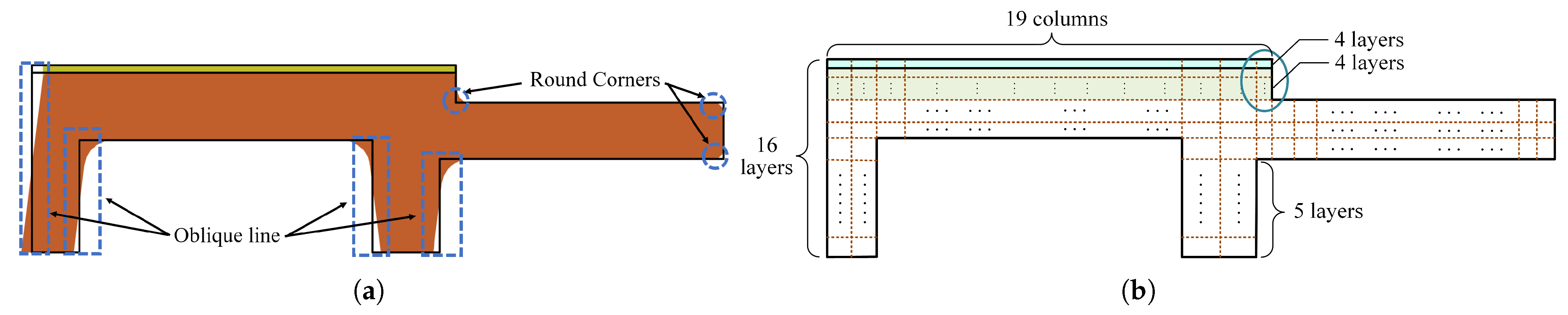
Figure 4a illustrates the simplified secondary structure configuration, where geometric complexities such as rounded corners and oblique edges are approximated by rectangular boundaries in the proposed LPTN model. Figure 4b presents the network distribution. The analytical domain is divided into a series of nodes, which represent the plate, the F-shaped rail and the air. The layer thickness of the mesh is related to the distribution of losses. In the plate region, because of the modulation function of the F-shaped rail, the flux travels through the whole plate; so, we consider a uniform layer thickness in the plate region, consisting of 4 layers and 19 columns.

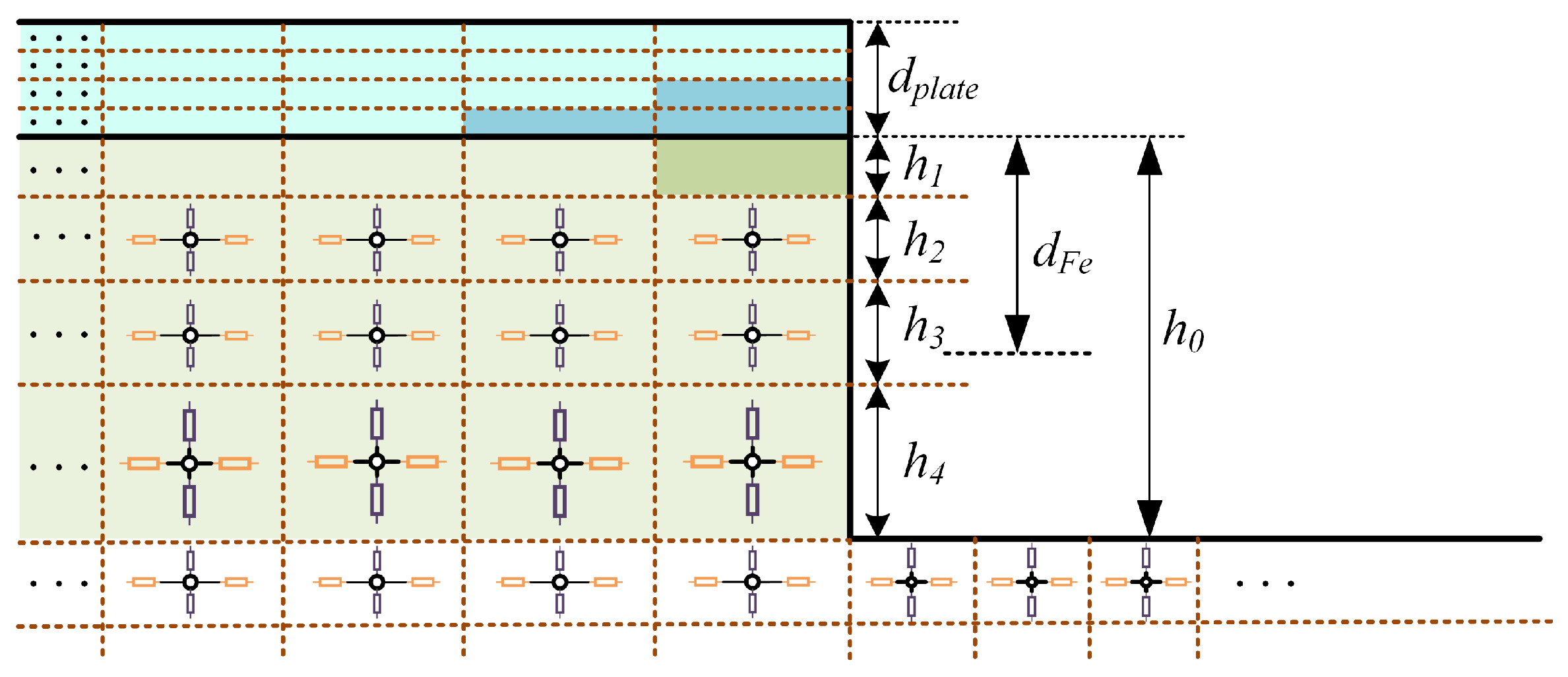
The layer in the rail region is different. Figure 5 shows details of the circle in Figure 4b, where four layers are deployed in the green region of the rail. Because of the skin effect, the magnitude of the flux density drops as the penetration depth increases. As a result, the distribution of losses in the vertical direction is non-uniform. Upon entering the F-shaped rail, the flux density is high, resulting in significant losses. As the depth increases, the flux density gradually decreases, leading to a reduction in losses. The boundaries of each mesh layer are set at the points where the flux density decreases to 25%, 50%, and 75% of its original value. The height of each cell is, respectively, $h_1$, $h_2$, $h_3$ and $h_4$. According to the definition of skin depth where the value reduces to $1/e$ of the original value, it is obvious that $h_1+h_2<d_{Fe}<h_1+h_2+h_3$, as shown in Figure 5.

Within each mesh, the flux density is assumed to be uniform, with its magnitude equal to the average of the flux density value of the upper and lower boundaries. Additionally, the losses are assumed to be proportional to the magnetic flux density.

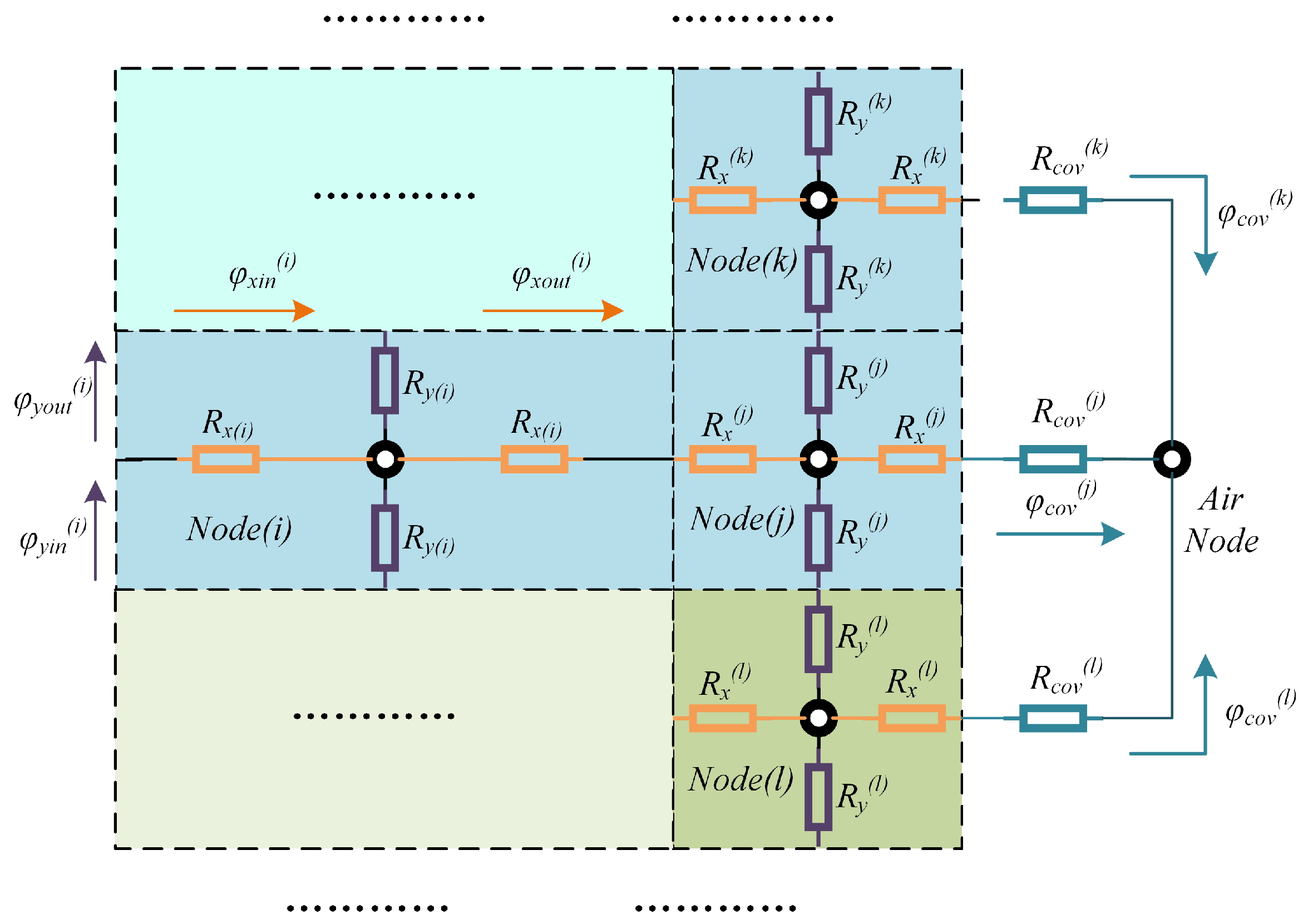
Figure 5 additionally presents the thermal resistance network within the system. Figure 6 details the complete network topology and nodal connections, where interface nodes (indicated by deeper blue and green hues) are specifically positioned at the contact surfaces between the conductive plate and F-shaped rail.

The thermal network incorporates both horizontal (orange) and vertical (purple) thermal resistances arranged in a cross configuration within each cell. Natural convection cooling is applied to all exposed surfaces, with air nodes connected to every surface node via convection thermal resistances (blue). Each cell features four heat flow paths, two input channels and two output channels, establishing thermal transport throughout the structure. Heat flow, represented by the symbol $\phi$, travels through nodes and eventually arrive at the air node to dissipate.

4.2. Heat Resistance Calculation

In this article, radiation heat transfer is neglected. Conduction heat resistance is calculated by

$$R_{Conduction}={\displaystyle \frac{1}{{\lambda }_T}}{\displaystyle \frac{L_T}{A_T}}$$

(20)

where $R_{conduction}$ is the conduction heat resistance and ${\lambda }_T$ is the thermal conductivity of the material. $L_T$ and $A_T$ are the length and section area of the heat transfer path.

For the natural cooling situation, convection heat resistance should be applied, which is calculated by

$$R_{Convection}={\displaystyle \frac{1}{h_T·A_T}}$$

(21)

where $R_{convection}$ is the convection heat resistance and $h_T$ is the convective heat dissipation coefficient, which is calculated as

$$h_T={\displaystyle \frac{N_u·{\lambda }_c}{D_e}}$$

(22)

where ${\lambda }_c$ is the thermal conductivity of the cooling medium, $D_e$ is the characteristic length and $N_u$ is Nusselt coefficient. In this article, $N_u$ is calculated by [35,36]

$$N_u=a{\left(G_r{P}_r\right)}^b$$

(23)

where a and b are the constants depending on different situations.

$G_r$ and $P_r$ are the Grashof number and Prandtl number, which are calculated by

$$G_r={\displaystyle \frac{g\mathsf{\Delta }T{\rho }_{fluid}^2{D}_e^3}{\left(273.15+T_{fluid}\right){\mu }_{fluid}^2}}$$

(24)

$$P_r=C_p{\mu }_{fluid}/\phantom{C_p{\mu }_{fluid}{\lambda }_c}{\lambda }_c$$

(25)

where g is the gravitational acceleration, ΔT is the delta temperature between the fluid and solid, ${\rho }_{fluid}$ is the density of the fluid, $T_{fluid}$ is the temperature of the fluid, ${\mu }_{fluid}$ is the dynamic viscosity of the fluid and $C_p$ is the heat capacity.

4.3. Transient Heat Balance Equation Establishment

For node i, at any time, the power that causes the temperature to increase equals to the power produced by itself, along with the heat transferred to i from other nodes, which can be expressed as [37]

$$C_i{M}_i{\displaystyle \frac{d{T}_i}{dt}}=P_i+\sum _{j=1,j\ne i}^n{\displaystyle \frac{1}{R_{ji}}}\left(T_j-T_i\right)$$

(26)

where $C_i$ and $M_i$ are the heat capacity and mass of node i; $T_i$ and $T_j$ are the temperatures of nodes i and j; $p_i$ is the power produced by node i; $R_{ji}$ is the heat resistance between nodes i and j and n is the total number of nodes.

Discretizing Equation (26) is necessary when calculating using a computer. The discretized equation also considers the constant temperature nodes, which is expressed as

$$G{T}^{\left(k\right)}=P+T_{en}-CM\left(T^{\left(k+1\right)}-T^{\left(k\right)}\right)/\phantom{CM\left(T^{\left(k+1\right)}-T^{\left(k\right)}\right)\mathsf{\Delta }t}\mathsf{\Delta }t$$

(27)

where G is the heat conductance matrix; $T_{en}$ is the temperature column vector; C and M are, respectively, the heat capacity and mass diagonal matrix; $T^{(k+1)}$ and $T^{\left(k\right)}$ are, respectively, the temperature column vector in time $k+1$ and time k. Δt is the step.

P is the power column vector. When calculating during a heating occasion, the values of elements in P are calculated by (18) and (19). When calculating during a cooling occasion, P equals the null vector.

4.4. Coupled Model Establishment

The SLIM system exhibits strong electromagnetic–thermal coupling behavior. The temperature distribution in the secondary conductive plate is primarily governed by electromagnetic induction from the primary winding. Conversely, this temperature distribution modifies the plate’s electrical resistivity, thereby influencing the electromagnetic field characteristics. This bidirectional interaction necessitates a coupled electromagnetic–thermal analysis for accurate system evaluation. 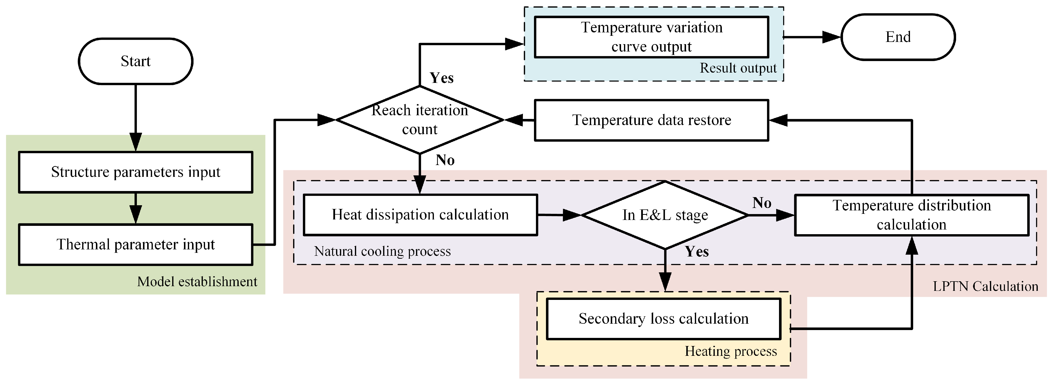Figure 7 illustrates the complete coupling methodology, demonstrating the implementation for periodic operating conditions.

The resistivity of the plate is the function of temperature, which can be evaluated by

$${\rho }_{plate}={\rho }_{plate20}\left(1+{\alpha }_{plate}\left(T-20\right)\right)$$

(28)

where ${\rho }_{plate20}$ is the resistivity of the plate in 20 °C, ${\alpha }_{plate}$ are the temperature coefficients and T is the temperature.

The conductivity of the plate is updated in each iteration. Subsequently, the plate with the updated conductivity is utilized for loss and temperature calculations. The resultant temperature, in turn, influences the next update of the conductivity of the plate. This is where the coupling analysis manifests.

As time progresses, the new temperature of the plate is obtained for each iteration and recorded. When the iteration is over, the variation in temperature is obtained.

The process of temperature merely rising and dropping is simpler than Figure 7 shows, which neglects the ‘In E&L stage’ decision. The ‘Temperature rising part’ or ‘Temperature dropping’ is then performed to obtain the temperature variation pattern.

5. FEM and Experiment Verification

In this part, three kinds of experiments that were conducted to verify the correctness of the coupled analytical model are presented. These are the SLIM stalling experiment, natural cooling experiment and SLIM periodic running experiment. FEM was conducted simultaneously and compared with the analytical model and experiment results.

5.1. Experiment Setup

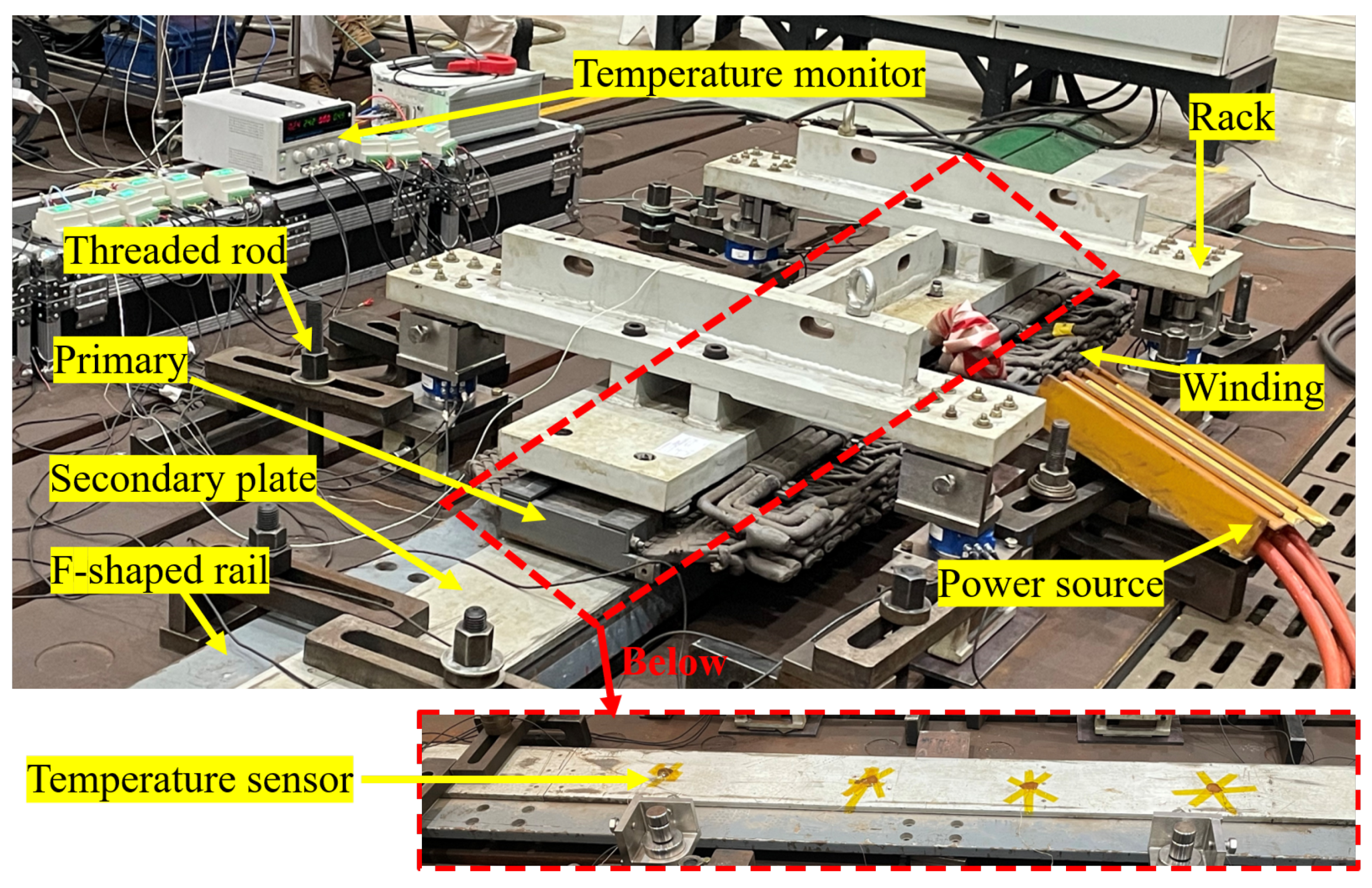
Figure 8 illustrates the experimental setup of the SLIM system. The primary winding assembly was mounted on an adjustable rack, with the air gap precisely controlled via threaded rods positioned at each corner. Temperature measurements were obtained using surface-mounted sensors on both the secondary conductive plate and F-shaped rail. To ensure measurement stability, all sensors were secured with high-temperature-resistant yellow insulation tape. Particular attention was given to rail temperature monitoring due to its significant influence on natural convection cooling performance.

The SLIM stalling test requires continuous power application for a predetermined duration while monitoring the plate temperature and structural integrity. The experiment is immediately terminated upon detection of any abnormal conditions, including plate deformation or smoke emission, to ensure safety and prevent equipment damage.

The natural cooling experiment was conducted immediately afterward. The SLIM remained stationary in a sealed, non-ventilated environment maintained at 25.0 °C ambient temperature. Throughout the cooling process, the plate’s temperature variations were continuously monitored and recorded with high precision.

The periodic running experiment simulates the temperature variation of the secondary plate under the actual maglev train shift conditions. The details are discussed in Section 5.5.

The temperature sensor, PT100, has a measurement range of −50 °C to 200 °C, with precision being 0.1 °C. The material of its probe is type 304 stainless steel. In addition, a three-core fluoropolymer is used for the lead wire to ensure high-quality information transmission.

The parameters of the SLIM prototype are shown in Table 1.

Table 2. Structure parameters of F-shaped rail.

Symbol	Description	Value	Unit
$W_1$	Width of pole	28	mm
$W_2$	Width of window	164	mm
$W_3$	Width of rail arm	140	mm
$h_0$	Height of protrusions	16	mm
$H_1$	Height of window	60	mm
$H_2$	Thickness of rail	36	mm
$H_3$	Height of rail arm	30	mm
$L_1$	F-shaped rail length	2000	mm

shows the parameter of the F-shaped rail.

5.2. Magnetic Field Analysis

It is worth mentioning that the EC model used for the calculation of losses is deduced under linear condition. However, huge current is applied to the SLIM according to Table 1, so the saturation level should be discussed to guarantee the accuracy of the EC model.

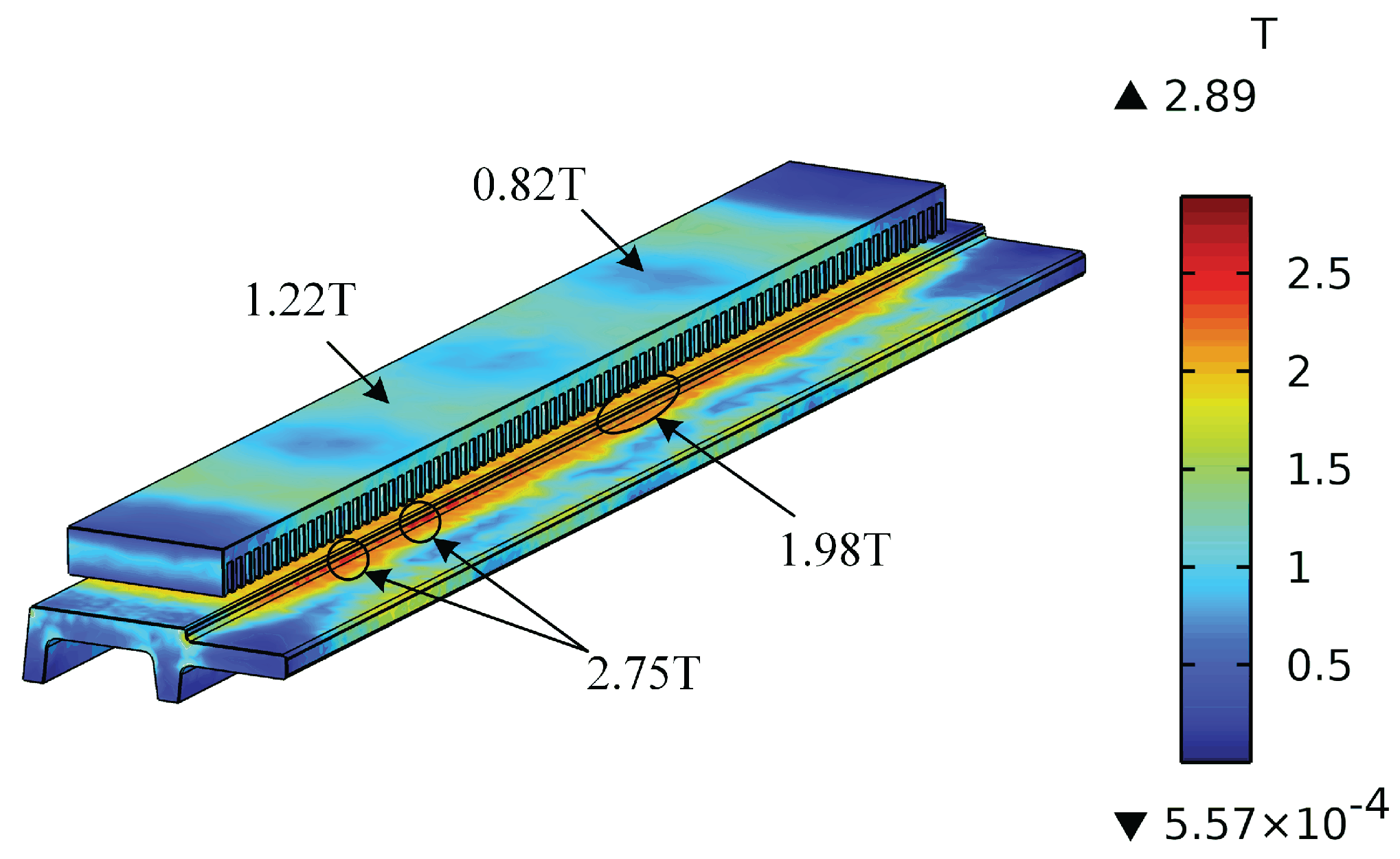
As a result, an FEM was conducted with the SLIM rated condition, as is shown in Figure 9.

While the local flux density reaches nearly 3 T in small regions such as rounded corners, these areas are sufficiently limited in size to negligibly affect overall magnetic saturation and electromagnetic performance. The primary core maintains an average flux density of approximately 1.3 T, while the rail’s upper layer exhibits about 2.0 T—both values approaching the 1.9 T saturation inflection point of the SLIM’s ferromagnetic material. This confirms that the system operates below deep saturation levels, validating the continued applicability of EC theory.

5.3. Temperature Rising Under Stalling Condition

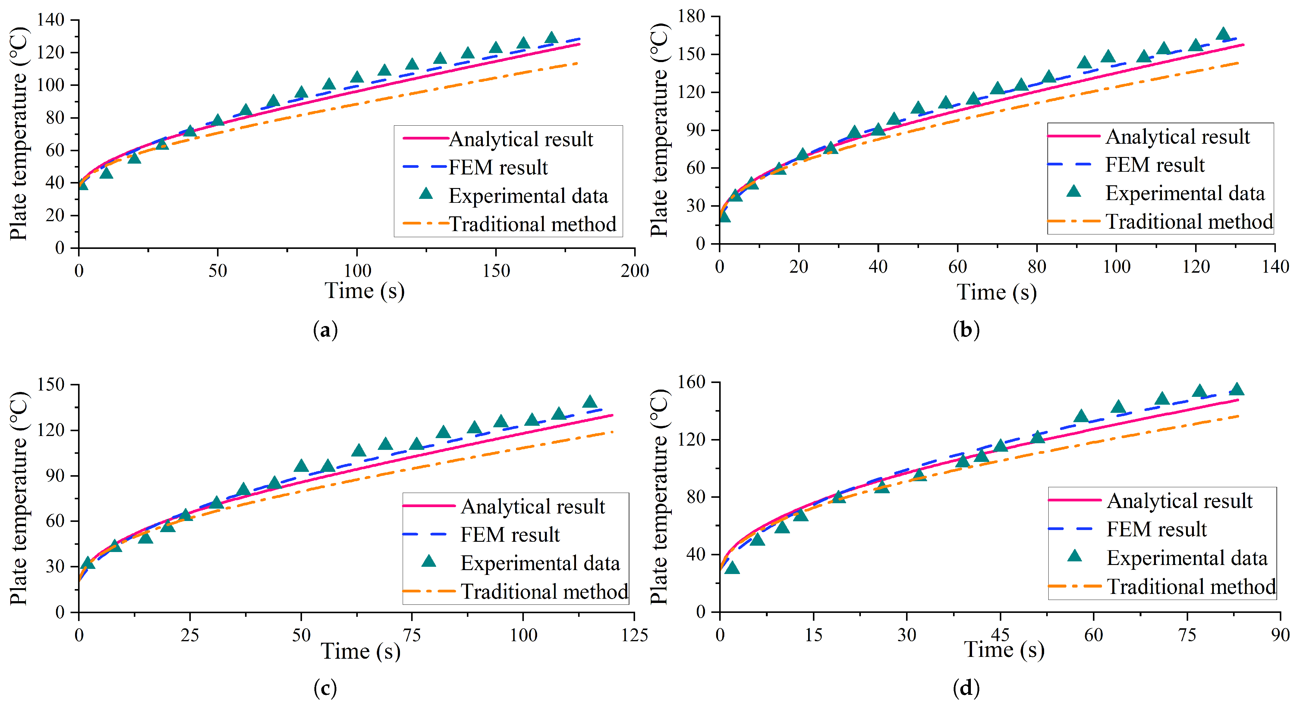
The result of the analytical coupled model, simulation and experiment are shown in Figure 10, which presents the temperature of the secondary plate rising with time under different air-gap lengths, frequencies and current values.

The plate temperature exhibits rapid temporal escalation, as demonstrated in Figure 10a, where temperatures exceed 120 °C within a 3 min interval. Experimental measurements, analytical model predictions, and FEM simulations show strong agreement, with a maximum observed deviation of 7.6% at t = 120 s. This discrepancy primarily stems from the experimental limitation of surface-only temperature measurements by sensors, whereas both numerical and analytical approaches compute volumetric temperature distributions. However, the plate’s minimal thickness ensures negligible thermal gradients between its interior and surface, resulting in the modest error observed.

The influence of different excitations to the temperature rising behavior can be obtained by comparing four figures of Figure 10. The influence of frequency can be obtained by (a) and (b). It takes 155 s and 68 s for the plate temperature to rise from 40.0 °C to 120.0 °C with frequencies of 8 Hz and 13.69 Hz. The eddy current and the heat power produced by it rise with increasing frequency, leading to a faster temperature rising rate. The frequency of the latter is almost twice as much as that of the former, and time for rising the same temperature is nearly half of the situation of 8 Hz. This can be a rough criterion for the result.

The current dependence is evident from comparing (b) and (c). When the current decreases from 330 A to 280 A, the temperature rise after 120 s reduces from 148.8 °C to 130.0 °C (from an initial 20.0 °C). This temperature reduction results from decreased eddy current generation and weaker magnetic flux in the secondary plate due to the lower primary current.

The air-gap length influences the performance of the motor and secondary loss. When the air-gap length reduces from 13 mm to 10 mm, the temperature of the plate rises in 80 s from 20.0 °C to 120.8 °C in Figure 10b and 29.6 °C to 145.1 °C in Figure 10d, though the thrust increases by air-gap length reduction.

The orange dashed lines in Figure 10 represent the temperature rising curve based on the uncoupled model, which was adopted in previous studies such as [6,7]. As can be seen from the figure, the difference between the coupled model/uncoupled model and the experimental result is small when the plate temperature is low, especially under 60 °C. Although it is in a high-temperature region, the difference is large. The average errors under 60 °C and above 60 °C are, respectively, 5.17% and 6.28% for the coupled model and 5.31% and 13.93% for the uncoupled model. This difference is mainly caused by the resistance of the secondary plate. At the beginning when temperature is low, the coupling effect is not strong. However, with the growth of temperature, the resistivity of the plate increases rapidly, which further enhances the heating power, so the temperature growth rate increasingly rises. In the paper, the temperature is always higher than 60 °C, where the coupled model shows greater quality than the traditional model. As a result, the coupled model proposed in this article is used to conduct the research.

5.4. Temperature Dropping Under Natural Cooling Condition

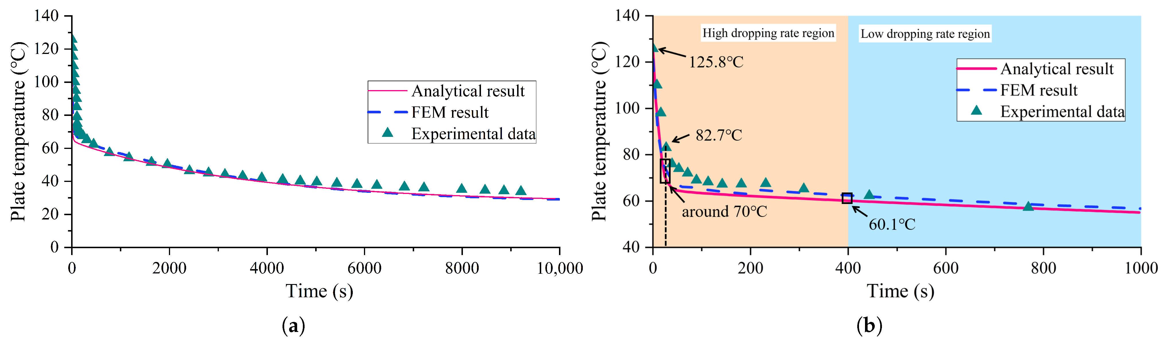
Figure 11 presents the natural cooling characteristics of the plate, with Figure 11b showing an expanded view of the cooling curve from Figure 11a. Both analytical and FEM results reveal a distinct two-phase cooling behavior: an initial rapid cooling phase where the temperature drops from 125.8 °C to 60.1 °C within 400 s, followed by a prolonged gradual cooling phase requiring 2.67 h to decrease from 60.1 °C to 29.8 °C. Experimental data confirm this nonlinear cooling trend, exhibiting similar rate variations.

Two primary factors govern this cooling behavior:

(1) The initial large temperature differential between the plate and ambient environment (25.0 °C) drives efficient heat transfer, with cooling rates diminishing as this gradient decreases. This explains the progressively slower temperature reduction, particularly in the final cooling stage.

(2) Thermal interaction with the F-shaped rail significantly influences the cooling process. The rail’s substantial mass and heat capacity maintain its temperature at approximately 70.0 °C, considerably lower than the initial plate temperature. Consequently, conductive heat transfer to the rail dominates the early cooling stage. Only after approximately 400 s, when the plate and rail approach thermal equilibrium, does natural convection become the predominant cooling mechanism.

The analytical model, FEM simulations, and experimental results demonstrate strong agreement across both rapid and gradual cooling phases. This agreement is particularly strong after 400 s during the slow cooling phase, where the maximum observed error is limited to 8.13%. The maintained agreement during the initial rapid cooling phase stems from proper consideration of the rail’s thermal influence, including accurate initialization of the rail temperature in our models. This comprehensive approach ensures reliable temperature prediction throughout the entire cooling process.

Moreover, the final temperature value of the analytical/FEM model (29.8 °C) being slightly smaller than that of the experiment (32.4 °C) is caused by the primary structure. In the experiment, primary is located only 13 mm above the surface of the plate, which negatively impacts the cooling condition and makes it harder for heat to dissipate through the plate’s upper surface, while the simulation setup neglects it and keeps the heat dissipation of all surfaces at the same value.

5.5. Temperature Variation Under Periodic Running Condition

The SLIM periodic running experiment was conducted to simulate the real operation condition of maglev commercial lines. During commercial operation, the primary of SLIM works for a period of time in the train’s E&L stage, which is when the temperature of the plate rises. During the W stage, no carriage arrives and the plate temperature drops by natural cooling. This is equivalent to SLIM not working.

There still exists a stage between the E&L stage when the passengers board the train. It is neglected because the time of this stage is very small compared to the W stage.

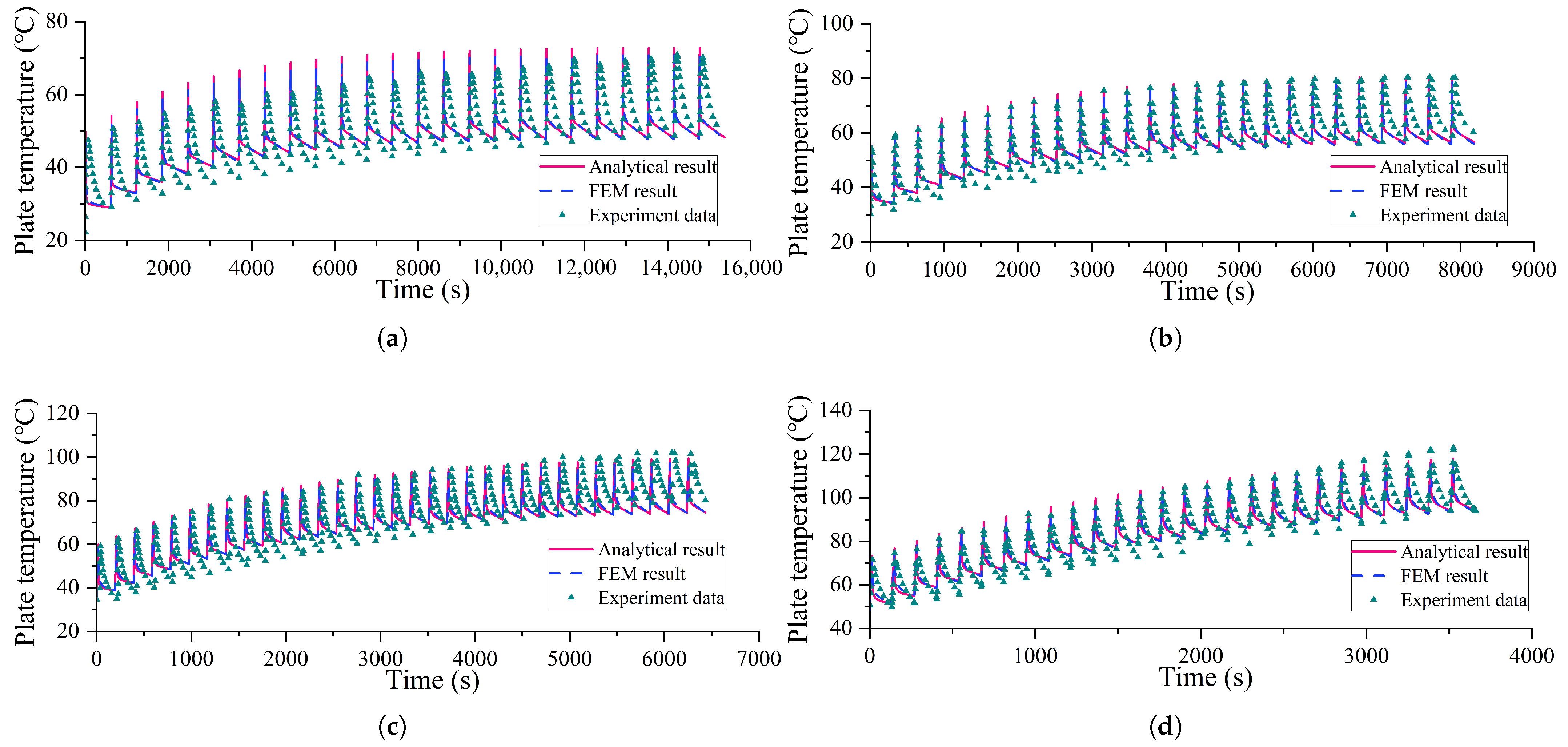
In the experiment, the SLIM working period lasts for 15 s; the times of stopping the working period are, respectively, 600 s, 300 s, 180 s and 120 s. The results are shown in Figure 12.

In Figure 12, the blue dotted line and the magenta line stand for the FEM and analytical results, respectively. These two present great agreements through the entire process. The experimental data, represented by green triangles, show the same trend with the FEM/analytical one.

The experimental results exhibit slightly higher temperatures than the analytical predictions across successive periods. This discrepancy arises from cumulative errors in rail temperature estimation between the experimental and analytical approaches. As discussed in Section 5.4, the F-shaped rail significantly influences the cooling characteristics, particularly during the rapid cooling phase. Minor deviations in rail temperature—caused by unavoidable experimental factors such as air currents or ambient temperature fluctuations—can propagate through multiple periods, leading to progressively larger temperature differences.

The temperature profile exhibits a distinctive cumulative pattern across operational periods. Each cycle consists of both heating and cooling phases, with the temperature increase during heating consistently exceeding the subsequent cooling decrease. This results in a net temperature gain per cycle during initial operation. However, the peak temperature progressively decreases over successive periods until the system achieves thermal equilibrium, where the heating and cooling magnitudes become equal.

This behavior stems from the temperature-dependent cooling efficiency. During initial cycles, when the temperature differential ($▵T=T_{plate}-T_{ambient}$) remains relatively small, the cooling capacity is insufficient to fully offset the heating effects, causing gradual temperature accumulation. As $▵T$ increases, the enhanced cooling efficiency eventually balances the thermal input, establishing steady-state conditions where heat generation equals heat dissipation.

In this article, we define the minimum temperature in the balanced period as $T_b$ and the maximum one is $T_{max}$. It is found that the value of $T_b$ and $T_{max}$ are different in four figures. The shift time is clearly related to this. Shorter shift time means shorter cooling time, and the dropping value is reduced. To reach the balanced status, the temperature of the plate will rise as high as possible to realize a high cooling efficiency, thus within a relatively short time will the dropping value become the same as the rising value.

Furthermore, it is found that the rising rate of $T_b$ to $T_{max}$ is different in four experiments, which are 43.6%, 39.9%, 32.7% and 25.8%, respectively. This is because with the growth of $T_b$, which are 48.0 °C, 56.2 °C, 74.7 °C and 93.89 °C in four experiments, the initial 15 s heating is conducted under better cooling efficiency, leading to lower rising rates.

6. Maglev Train Optimization

Section 5 validates the proposed model. In this section, the model is used to conduct several optimizations about the maglev train based on the temperature constraints. Several studies [38,39] conducted optimizations about the structural parameters and outer excitation of the linear induction motor while keeping the running condition constant. In this article, however, more attention is paid to the optimization under the periodic running condition of SLIM.

It is easy to see that the $T_b$ and $T_{max}$ are related to heating time $t_{EL}$ and cooling time $t_W$, which are also the times of the train’s E&L stage and interval shift. Furthermore, the adoption of copper, which has higher conductivity compared to aluminum, for the secondary plate is also discussed.

6.1. Shift Interval Time Optimization

Apart from the results in Section 5.5, several analyses with different shift interval times were also conducted by the coupled model with $t_{EL}$ being 15 s, the results of which are listed in

Table 3. Shift interval time and resultant temperature and thrust.

${\mathit{t}}_{\mathit{W}}$ (s)	${\mathit{T}}_{\mathit{b}}$ (°C)	${\mathit{T}}_{\mathit{max}}$ (°C)	Rate (%)	Thrust (kN)
600	48.0	69.9	43.6	1.73
500	49.8	70.2	42.6	1.73
400	52.8	74.6	41.2	1.75
300	56.2	78.6	39.9	1.76
180	74.7	98.6	32.7	1.81
120	93.89	117.4	25.8	1.85
80	145.03	167.8	15.6	1.94
50	208.11	230.9	10.6	2.01
20	450.05	470.3	4.5	2.02

.

From Table 3, we find that the $T_b$ is almost the same in occasions of $t_w$ being 600 s, 500 s and 400 s. This can be explained by the fact that the $t_W$ is long enough for the rate of temperature dropping to transition from the high-dropping-rate region and into the low-dropping-rate region. The time when 600 s and 500 s exceed 400 s is only spent when the temperature drops at a low rate. As a result, their equivalent cooling effects will not be different due to the addition of 100 or 200 s, and the $T_b$ of these three cases are almost the same. The $T_{max}$ and rising rate are also resultant the same with the same heating time and power.

The thrust variation due to the temperature effect is also calculated according to Equation (15). It is obtained that the thrust of SLIM in ambient temperature is 1.59 kN. Table 3 presents the thrust under different shift interval times. It can be concluded that with the growth of $T_{max}$, the thrust increases by at least 8.8%. That is because the temperature effect increases the resistivity of the secondary plate. Although the secondary current decreases by $R_2$, the thrust initially rising for $R_2$ plays a dominant role.

To obtain insights on this relationship, a fitting by the above data was conducted. Figure 13 shows the $T_b$ and $T_{max}$ points under certain shift interval times and the fitting curve between $t_W$-$T_b$ and $t_W$-$T_{max}$.

It is clear that an inverse proportional functional relationship exists between points. So, an expression of $y=a/(x+b)+c$ is adopted to fit. Shift interval time $t_W$ equalling infinity means a long enough time for natural cooling. Under this circumstance, the coefficient c for balanced temperature $T_b$ equals to the ambient temperature, which is 25.0 °C in the experiment. For c, $T_{max}$ equals 48.6 °C, which is calculated by heating for 15 s from 25 °C.

Temperature reaches infinity when $t_W$ approaches 0 s for no time of the cooling period. Therefore, the coefficient b equals to 0. After confirming b and c, the analytical expressions and a are obtained by the MATLAB curve fitting calculation, the results are listed as

$$T_b=8645/\phantom{8645t_w+25.0}{t}_w+25$$

(29)

$$T_{max}=8583/\phantom{8583t_w+48.64}{t}_w+48.6$$

(30)

Based on the analytical expression, we can easily calculate the $t_W$ under the limitation of $T_{max}$ being 170.0 °C, which is 70.7 s. Under this shift interval time arrangement, the $T_b$ is 147.3 °C. Danger occurs when $T_{max}$ is higher. As a result, 70.7 s is selected to be the theoretically minimal and optimal shift interval time for the Maglev train shift arrangement. Under this arrangement, the thrust reaches 1.94 kN. A 22.0% increase occurs due to the temperature.

6.2. Material Optimization

In conventional engineering practice, aluminum is typically selected for the secondary plate due to its cost-effectiveness and manufacturing maturity. However, copper’s superior electrical conductivity suggests potential performance advantages when employed as an alternative plate material. This study therefore investigates the technical and economic feasibility of implementing copper secondary plates in SLIM systems.

In this analysis, the structural parameters of the copper plate remains the same with the aluminum plate. $t_W$ and $t_{EL}$ are 300 s and 15 s, respectively, for the simulation of a typical metro shift arrangement. This means that in the analytical model, firstly, the motor runs for 15 s to simulate the train entering and leaving the stage. The next 300 s are deployed to simulate the waiting period when natural cooling plays its role. The result is listed in

Table 4. Influence of plate material to temperature and thrust.

Material	${\mathit{T}}_{\mathit{b}}$ (°C)	${\mathit{T}}_{\mathit{max}}$ (°C)	Rate (%)	Thrust (kN)
Aluminum	56.2	78.6	39.9	1.76
Copper	44.6	61.3	37.3	1.30

, from which smaller values of $T_b$ and $T_{max}$ are obtained compared to the one when aluminum is adopted. By adopting copper, the balanced temperature and maximum temperature drops by 20.64% and 22.01%.

The thrust performance is also affected by changing the plate material. By applying copper, the thrust drops by 26.1% from 1.76 kN to 1.30 kN.

The analysis demonstrates that while copper plate implementation reduces the maximum temperature, it concurrently degrades thrust performance. Given copper’s substantial cost premium, this approach may be selectively justified only in specific operational scenarios—particularly for railway segments adjacent to stations where reduced thrust requirements prevail.

6.3. Carriage Number Optimization

Adopting more carriages or extending carriage length can improve the train capacity. However, heating time increases along with increasing carriage number/length as the primary length of the SLIM above a certain point on the secondary plate increases, and the duration of the eddy current existing at that point also increases under the same maglev train speed. This fact is treated as heating time $t_{EL}$ extending in the analysis. Furthermore, we reckon that $t_{EL}$ is proportional to the length of the carriages, details of which and its result of $T_b$ and $T_{max}$ are listed in

Table 5. Carriage number and resultant temperature and thrust.

${\mathit{N}}_{\mathbf{ca}}$	${\mathit{t}}_{\mathbf{EL}}$ (s)	${\mathit{T}}_{\mathit{b}}$ (°C)	${\mathit{T}}_{\mathbf{max}}$ (°C)	Rate (%)	Thrust (kN)
1.5	7.5	38.5	53.0	37.8	1.68
3	15	56.2	80.9	43.9	1.76
4.5	22.5	71.1	101.2	42.3	1.81
6	30	89.0	126.0	41.5	1.87
7.5	37.5	104.1	145.9	40.1	1.91
9	45	118.9	165.2	38.9	1.94

. In the table, a $t_W$ of 300 s is usually adopted by a typical metro schedule.

It is the time of entering and leaving that matters but not the carriage number, a part of which was selected to be a non-integer to simulate a different $t_{EL}$. In reality, these circumstances are realized by a single carriage length extending.

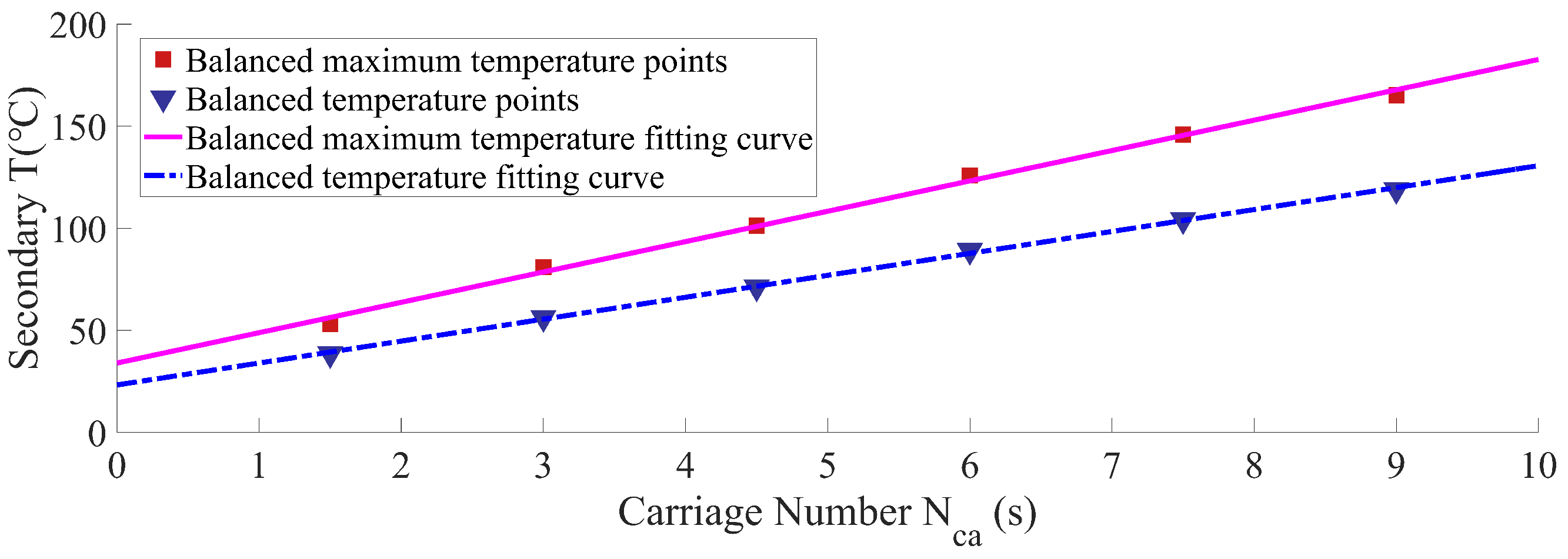
The resulting points and their trend curves are shown in Figure 14. The proportional relationship between points can be clearly observed and the fitting curve expressions for both $T_b$ and $T_{max}$ with carriage number $N_{ca}$ are listed as

$$T_b=10.74N_{ca}+23.6$$

(31)

$$T_{max}=14.87N_{ca}+34.0$$

(32)

The intercept of both $T_b$ and $T_{max}$ expressions in the y axle represent the ambient temperature because, at this moment, there is no heating time. The intercept of $T_b$ is 23.6 °C, which is similar to the experiment temperature. But the counterpart of $T_{max}$ reaches 34.0 °C, which is higher than the former one. This is considered as an experimental and data-processing error that cannot be avoided.

From Equations (31) and (32), under the safety temperature boundary, an optimal carriage number is calculated to be nine if it is rounded up, while $T_b$ and $T_{max}$ are 120.3 °C and 167.8 °C. The thrust under this arrangement is 1.94 kN, where a 22.0% increase is reached. If not, the length of the carriage can be equivalent to the length of 9.15 carriages, while the $T_b$ and $T_{max}$ are 121.9 °C and 170.0 °C.

The rising rate is found to be 40%, as presented in Table 5. This is mainly caused by $t_W$, which reaches 300 s in the analysis. The temperature dropping rule is discussed above and it is clear that 300 s is long enough to complete the high-dropping-rate region; the resultant temperature is low, and thus, the rising rate is almost the same. Furthermore, it can also be predicted that if $t_W$ becomes smaller, the rising rate will decrease as the data in Table 3 decrease.

7. Conclusions

The SLIM of a medium–low-speed maglev train normally runs in an equivalent periodical condition. The temperature of the secondary plate rises rapidly in the E&L stage when the slip is high and drops in the shift interval time, which complicates the analysis. Furthermore, the conductivity of the plate varies along with the temperature, which affects both the power of heating and the thrust. In order to calculate the temperature variation more precisely, a magneto-thermal coupled model combining EC considering end and edge effects and LTPN are introduced in this paper, where the mesh of LPTN is well designed to consider the skin effect. FEM and three kinds of experiments were conducted to validate the model. Then, based on the model, the optimizations for shift interval time, material selection and carriage number were conducted and the resultant thrust impacts were discussed. The conclusions are as follows:

(1) The minimum shift interval time of the maglev line is 70.7 s. The resultant thrust increases by 22.0% due to the temperature effect.

(2) By replacing the aluminum plate with a copper plate, $T_b$ and $T_{max}$ drop by 20.64% and 22.01%. The thrust decreases by 26.1%. Due to the high cost of cooper, this method can be applied to rail sections near stations where thrust demand is small.

(3) A carriage number of nine is optimal. The thrust increases to 1.94 kN by a temperature effect.

This work provides a temperature calculation method of a secondary plate and an optimal selection of shift time, plate material and carriage number. Because this working condition reoccurs in every station, the results are valid for the entire route. After the optimization, the passenger capacity of the maglev line can be improved thermally safely with no extra cost. If the passenger flow exceeds the maximum capacity achievable by increasing train shift frequency or adding more carriages, replacing the aluminum plate with copper is a reliable method. Costs will indeed increase, but replacing only the plate materials in the entry/exit sections can maximize cost savings.