Construction of a Surface Roughness and Burr Size Prediction Model Through the Ensemble Learning Regression Method

Abstract

It is well understood that burr size and shape, as well as surface quality attributes like surface roughness in milling parts, vary according to several factors. These include cutting tool orientation, cutting profile, cutting parameters, tool shape and size, coating, and the interaction between the workpiece and the cutting tool. Therefore, burr size cannot be formulated simply as a function of direct parameters. This study proposes an ensemble learning regression model to accurately predict burr size and surface roughness during the slot milling of aluminum alloy (AA) 6061. The model was trained using cutting parameters as inputs and evaluated with performance metrics such as mean absolute error (MAE), mean squared error (MSE), and the coefficient of determination (R²). The model demonstrated strong generalization capability when tested on unseen data. Specifically, it achieved an R² of 0.97 for surface roughness (Ra) and R² values of 0.93 (B5, B8), 0.92 (B2), 0.86 (B1), and 0.65 (B4) for various burr types. These results validate the model’s effectiveness despite the nonlinear and complex nature of burr formation. Additionally, feature importance analysis via the F-test indicated that feed per tooth and depth of cut were the most influential parameters across several burr types and surface roughness outcomes. This work represents a novel and accurate approach for predicting key surface quality indicators, with significant implications for process optimization and cost reduction in precision machining.

1. Introduction

As manufacturing processes advance, fabricating precision parts requires careful attention. High-quality items must be made precisely to match the design details and kept affordable. The manufacturing steps need a thorough understanding, and parameter tweaking is essential to meet these demands [1]. The quality of surfaces and edges plays a critical role in the machining process, with surface roughness, particularly Ra, and the formation of burrs being key factors. Controlling surface roughness and minimizing burr size are crucial objectives across various industries, as they significantly impact the final cost of machined parts. As noted by Gillespie [2], the cost of deburring and edge treatment for precision parts can reach up to 30% of the total expenses. Moreover, automating this secondary process proves challenging, creating potential production delays [3]. To effectively remove burrs from machined edges and holes, an undesirable and costly secondary procedure is required. Several factors, such as burr size, location, and the material involved, influence the intricacy and difficulty of these deburring tasks [4].

Research into burr mechanisms spans more than forty years. As previously indicated, the occurrence of milling burrs involves a complicated process where burrs form as the cutter penetrates and exits the material. Nakayama and Arai [5] categorized milling burrs according to the direction of burr formation and cutting edge. They identified milling burrs through observation, analyzing how burrs form when the cutting tool engages with and disengages from the material. Several process parameters influence face milling burrs, which were extensively examined [6,7,8,9,10,11,12,13,14]. To distinguish between different burr sizes on part edges, the concepts of primary burr and secondary burr were introduced by Kishimoto et al. [13]. They observed that secondary burrs are smaller than the depth of the cut, while primary burrs are larger. Chern [14] investigated burr development in the face milling of AAs and concluded that the formation of secondary burrs is significantly affected by the depth of cut and the feed rate. Additionally, most studies in this field focus on burr height. From a deburring viewpoint, burr thickness is more important as it dictates the time and method required for deburring. Only a few studies utilized statistical analysis to identify the main process parameters affecting burr size [15]. A more systematic approach would advance the understanding and control of burr formation, making it easier to predict and manage in machining operations [16,17].

Except for a few works [17,18,19], limited data exist on how main process parameters impact the creation of slot milling burrs. The complexity of these burrs may arise from their formation in three distinct ways. They exhibit various forms, including feed direction burrs, entrance and exit burrs, sideward burrs, and cutting direction burrs on the eight edges of the machined component (see Figure 1). Unlike face milling, where multiple passes of the tool can eliminate burrs made by prior passes, end milling does not usually achieve this effect. As a result, both side and top burrs may persist on the part, potentially leading to various problems. The most minor burrs are the entrance side burr near the up-milling side and the burr at the entrance’s bottom. Medium-sized burrs consist of the top burr along the up-and-down milling sides, the entrance side burr on the down-milling side, and the exit side burr on the down-milling side. The giant burrs are the exit side burr along the up-milling side and the exit bottom side burr. Through understanding these types and sizes, better strategies can be developed to address burr formation in slot milling [14]. In this work, along with Figure 1, B1, B2, B4, B8, and B5 will be studied.

With the development of technology, new computational methods, such as neural networks, fuzzy logic, and their integration with optimization methods, have been proposed and investigated. In studying the modeling and forecasting of Ra during milling, Karayel [20] developed and trained a multilayer feedforward ANN model [21], resulting in an average error of only 0.023. Similarly, Gupta et al. [22] created a hybrid ANN-based GA model. AI-driven models, like radial basis function networks (RBFNs), fuzzy hybrid networks, and GA, have demonstrated solid accuracy and dependability [23,24]. Barua et al. [25] implemented an RSM-based method to assess how cutting conditions affect Ra in machining AA 6061-T4, achieving a reliability rate of 90% under specific conditions. However, as far as the authors know, because of the many interactions related to burr formation, these methods have not been very successful with the burr mechanism. As a result, machine learning methods have gained attention in the last decade. Machine learning is a subdivision of computational science that is based on learning data classification based on the gained understanding and the learning gained on computational-based principles of Artificial Intelligence [26]. Despite the positive aspects of this approach, machine learning has not been widely used in predicting and controlling surface quality and edge indicators.

During this study, one of the advanced machine learning approaches, so-called the optimized ensemble learning framework, was used for an accurate prediction of the surface roughness and burr height in the slot milling of AA 6061. The effects of each input parameter on burr formation and surface roughness were also investigated. In the proposed model, cutting parameters were used as the inputs. At the same time, the main outputs were surface roughness and burr height, which were used for training, validation, and testing according to defined strategies. The predicted values were evaluated using MAE, MSE, and the correlation of determination (R²). What sets this work apart is the application of an ensemble machine learning approach specifically optimized for the dual-objective prediction of burr height and surface roughness—something not previously reported in the context of slot milling. This novel integration enables a more accurate and generalized model that can handle previously unseen data, improving reliability in real-world manufacturing scenarios. Furthermore, by identifying the relative influence of input parameters through explainable AI tools, this study not only enhances prediction accuracy but also contributes to a deeper process understanding, offering actionable insights for process optimization. No similar type of work was reported in the open literature to handle unseen data. This work plans to remedy the lack of knowledge indicated.

2. An Overview of Surface and Edge Quality

As previously mentioned, several valuable indicators exist for assessing the quality of manufactured products. Surface roughness and burr formation are two of the most crucial indicators, and each will be briefly discussed in the following section.

• Burr formation.

Burrs created during machining significantly affect overall costs [27]. Thus, they must be removed at a later stage. Burr removal is not a value address process [15]. Complete burr removal burrs is a crucial and costly operation. Selecting the best methods and understanding the key parameters is necessary to reduce deburring costs [28]. Knowing the burr formation process helps control burr size. It is more effective to prevent burrs during machining than deal with them later [29]. Gillespie, an expert, noted that burr technology is complex [30]. Burrs on a workpiece cause numerous issues. They hinder assembly, harm dimensional accuracy, damage surface finishes, and increase production time and costs. Workers’ and consumers’ safety is at risk. Additionally, burrs can lead to electrical short circuits, lower cutting performance, reduce tool lifespan, and affect the appearance of components. Even during machining, burrs strike cutting edges and cause groove wear. This wear then speeds up burr growth. Therefore, controlling burr formation and minimizing the subsequent removal steps are vital for efficient manufacturing [30].

• Surface roughness.

Surface roughness is a crucial measure of product quality and often a technical need for mechanical components [31]. Deteriorated surfaces generally wear out faster and have more friction than smoother ones. Thus, achieving high-quality surfaces is vital for precision parts. Roughness impacts how products interact with their surroundings. Although reducing surface roughness is challenging and costly, it is usually necessary. Lowering roughness drastically increases production costs, leading to a compromise between cost and performance. Fine-tuning the milling process is tricky because of numerous controlling factors. Any slight change affects the process significantly. Hence, it is crucial to grasp the elements influencing the process to identify variation trends. Enhancing surface quality remains a complex issue, affecting the broader use of this technology [32].

3. Modeling Approach

As mentioned earlier, the complexities of prediction involve multiple layers and interactions between parameters related to burr formation and surface roughness, making it impossible for single-model neural network techniques to learn different patterns. Single-model-based regression approaches demonstrated exceptional accuracy during validation. They used a subset of the data for validation and the remainder for training. However, they were unsuccessful with new, unseen datasets. On the other hand, despite being nonlinear methods, neural networks rely heavily on stochastic training. This reliance makes them highly sensitive to the specific traits of the training data. Consequently, they exhibit high variability and incorrect predictions when applied to different datasets [33].

To overcome this limitation, Liu and Yao [34] introduced ensemble learning via Negative Correlation, which was later integrated with an evolutionary programming framework. This approach was rebranded as Evolutionary Ensembles with Negative Correlation Learning [35] and used by Breiman [36] and Rodriguez [37]. The primary benefit of ensemble learning over single models lies in its ability to boost the stability and precision of regression predictions. Unlike single models, multiple models are trained together, reducing prediction variance and improving the reliability and quality of these predictions [33]. The initial phase in ensemble learning is the preprocessing module. Its main objective is to prepare the data for training, incorporating various normalization techniques. These techniques include zero-mean normalization, logarithmic function transformation, normalization, and quantile normalization. Overall, ensemble learning offers a promising solution by addressing the shortcomings of single-model approaches and neural networks, ensuring improved outcomes in regression tasks [33].

The Min-Max normalization technique was used to scale data features to 0 to 1. It adjusted input parameters such as depth of cut, speed, feed per tooth, and tool coating. In total, 54 data points were collected for the surface roughness output parameter, along with each of the five burr formation output parameters. The decision tree method is a practical approach to pinpointing the key traits needed to gain insights. It examines the ratio of report facts and the Gini coefficient at each split until the terminal node target is achieved [38,39,40,41,42]. Several measures were employed to establish the weighting of input factors: information gain [43], the information gain ratio [44], and the Gini coefficient [45]. Information gain (Equation (4)) calculates the difference between the original and new expectation data, while the information gain ratio includes the split information value to avoid bias. The split information value represents the potential data from dividing the training dataset into several parts based on attribute A. The Gini coefficient (Equation (3)) gauges sample impurity, and the average Gini index is used to pick the most relevant trait at every calculation step, acting as the division attribute. Info(D) denotes original information, and Info_A(D) indicates updated information. The split information value shows the potential data from splitting the training dataset D into portions related to attribute A’s outcomes [46].

$$Gain\left(A\right)=Info\left(D\right)-{Info}_A\left(D\right)$$

(1)

$$GainRato(A)={\displaystyle \frac{Gain\left(A\right)}{SplitInfo\left(A\right)}}={\displaystyle \frac{Info\left(D\right)-{Info}_A\left(D\right)}{{\sum }_{j=1}^v\frac{\left|D_j\right|}{\left|D\right|}-{log}_2\left(\frac{\left|D_j\right|}{D}\right)}}$$

(2)

$$Gini\left(D\right)=1-{\sum }_{j=1}^v{p}_i^2$$

(3)

Regression tree ensembles are a potent machine learning tool for predictive modeling. They work well with imbalanced datasets [47]. Despite their flexibility, it is essential to agree on the best way to construct an ideal model [48]. Bagging and boosting are ensemble methods that enhance decision tree performance [49,50]. This study used Lsboost for the ensemble regression [51]. Bagging fits models on bootstrap samples, and multiple replications of the original training set exist. Combining these models reduces the variance, avoiding overfitting [47,48,49,50,51,52,53,54]. The dataset was resampled through replacement techniques, creating multiple aggregated decision tree models [55]. Each dataset was employed to construct and validate a decision tree model. The outcomes from these models were then aggregated by averaging their results, as shown in Equation (4). In this equation, y_i is the result from the i-th decision tree model, y is the expected outcome of the final model, and n is the total number of decision tree models. This process led to a comprehensive and robust predictive model that performed well across various datasets. The approach ensured accuracy and generalization, making it a reliable choice for predictive tasks [46].

$$y={\displaystyle \frac{\sum _{i=1}^n{y}_i}{n}}$$

(4)

In contrast, boosting in machine learning is a technique where a weak algorithm is trained repeatedly on different versions of the initial training set. By reweighting each version, the algorithm corrects previous mistakes and grows stronger. Lsboost is a tree-based method to build a solid regression model. It uses gradient boosting combined with a square loss function, represented by Equation (5) [56]. The target value y is the ongoing cumulative output ‘y_i’, shown in Equation (6). At the same time, ‘F’ is the actual training output, representing the true values observed during the training phase of the model. It compares against the model’s predictions to evaluate performance [57]. By adding trees and adjusting the sample weights, Lsboost develops a strong ensemble model [58]. Equation (7) [59] reduces the loss by applying the current time residual error ‘F’. Equation (8) [57] helps find the combination coefficients. To minimize the square loss using gradient descent, Lsboost constructs regression trees step by step. A new tree joins the ensemble in each step. The loss function’s negative gradient fits the pseudo-residuals. The learning rate, controlling each tree’s influence on the final prediction, is crucial. It reduces the trees’ output, avoiding overfitting. By combining its elements effectively, Lsboost aims to predict with higher accuracy, ensuring the model remains resilient against errors and performs better with each iteration [46].

$$L\left(y·F\right)={\displaystyle \frac{{(y-F)}^2}{2}}$$

(5)

$$y_i{=\beta }_0+{\sum }_{j=1}^{i=1}{\beta }_i{h}_j+{\beta }_i{h}_i=y_{i-1}+{\beta }_i{h}_i$$

(6)

$$E={\sum }_{t=1}^N[{\beta }_i{h}_i^t-{\widehat{F}}^t]$$

(7)

$${\displaystyle \frac{\partial E}{\partial {\beta }_i}}=0$$

(8)

Moreover, Bayesian optimization was applied to find the hyperparameter values that minimize MSE. This method estimates the mean squared error through a Gaussian process model and updates the model with error evaluations at each step [33]. The complete dataset was divided into three sets to build the prediction model. One part was used for training, another for validation, and the remaining portion was set aside as unseen data to evaluate the model’s performance. This division separated 10% of the data from the dataset as unseen data, allocating 15 to 25% of the remaining data for validation and using the rest to train the prediction model. Various methods, such as cross-validation and holdout validation, were used to evaluate the predictive model’s performance, and both demonstrated acceptable performance in validation. The prediction models were assessed using various metrics, such as MAE, MSE, and R². The performance of each index was evaluated using Equations (9)–(11) [60,61,62]. Figure 2 shows the flow chart for developing the Optimized Ensemble Learner framework.

$$MAE=\left({\displaystyle \frac{1}{N}}\right){\sum }_{i=1}^N|y_{{exp}_i}-y_{{pred}_i}|$$

(9)

$$MSA=\left({\displaystyle \frac{1}{N}}\right) ({\sum }_{i=1}^N{\left(y_{{exp}_i}-y_{{pred}_i}\right)}^2$$

(10)

$$R^2={\left({\displaystyle \frac{\sum _{i=1}^N(y_{{exp}_i}-{\overline{y}}_{exp})(y_{{pred}_i}-{\overline{y}}_{pred})}{\surd \left(\sum _{i=1}^N{\left(y_{{exp}_i}-{\overline{y}}_{exp}\right)}^2\sum _{i=1}^N{\left(y_{{pred}_i}-{\overline{y}}_{pred}\right)}^2\right) }}\right)}^2$$

(11)

where, in all equations, N denotes the number of data samples. The terms y_(pred_i) and y_(exp_i) refer to the predicted and experimental values. Additionally, $\overline{y}$_exp and $\overline{y}$_pred represent the average values of their respective groups. Specifically, y_(exp_i) is the actual (experimental) value for the i-th sample in the dataset, while y_(pred_i) is the predicted value for the i-th sample generated by the model. $\overline{y}$_exp is the mean of all experimental values, calculated as the sum of all y_(exp_i) values divided by the total number of data points (N), and $\overline{y}$_pred is the mean of all predicted values, calculated as the sum of all y_(pred_i) values divided by the total number of data points (N). These terms are used in calculating performance metrics like R², where they help assess the model’s ability to predict outcomes accurately by comparing the predicted values to the actual values in the dataset [46,63,64,65].

4. Experimental Studies

In many industrial applications, there is a substantial demand for the continuous development of new materials and the ability of engineers to manufacture complex parts within tighter tolerances. From this perspective, machining rare materials, such as titanium and aluminum alloys, is important. Consequently, detailed research has been carried out on the characterization and machining of titanium alloy [66,67]. In this study, we also specifically examined experiments involving aluminum alloys. The AAs 6061-T6 and 2024-T351 were chosen for the tests (

Table 1. Cutting parameters and their levels.

Experimental Parameters	Level
	1	2	3
A: Cutting speed (m/min)	300	750	1200
B: Feed per tooth (mm/z)	0.01	0.055	0.1
C: Depth of cut (mm)	1	-	2
D: Tool coating	TiCN	TiAlN	TiCN + Al2O3 + TiN
E: Material	Al 6061-T6	-	Al 2024-T321

). The cutting experiments were conducted on a 3-axis Huron CNC machine tool, featuring 50 kW of power, a maximum speed of 28,000 rpm, and a torque of 50 Nm. HURON CANADA Inc., Longueil, Québec, Canada, provided the CNC machine. The rectangular parts were machined for this purpose. A multilevel, full-factorial experimental design, 3³ × 2², was opted for in this research (Table 1). The cutting tool and workpiece materials were categorized qualitatively, while the other variables were treated quantitatively. In total, 108 experiments were conducted under dry milling conditions, with three flute-coated carbide end milling tools (Z = 3), a Helix angle (β) of 30°, and a tool diameter (D) of 19.05 mm. The experimental procedures were conducted again, resulting in 216 tests. Iscar carbide inserts with the coating listed in Table 1 were used. A high-resolution camera paired with an optical microscope was used to capture the burr images. Measurements of burr sizes were based on the recorded images from the microscope. The burr size was determined by taking the average of four thickness readings (B_t) and the maximum height value (B_h). After cutting operations, the most widely used roughness parameter, Ra, was measured using the surface profilometer Mitutoyo SJ 400. The profilometer was provided by Mitutoyo Corporation, Kawasaki, Kanagawa, Japan.

Assumption

Specific challenges exist in machining AAs. These materials easily stick to the tool surface, leading to burr formation inside holes and on part edges.

To conduct the experiments, several assumptions were made:

• Chatter was assumed to be absent during slot milling tasks.
• Vibrational effects and tool dynamics were not considered.
• Initial evaluations confirmed the stability of cutting operations.
• It was presumed that deflections in both the tool and workpiece were negligible, maintained through sturdy fixtures.
• After each test, a new cutting tool was employed to avoid discrepancies due to tool wear.

5. Results and Discussion

An ensemble learning regression algorithm generated a dataset of 54 entries to develop a prediction model. While a larger dataset would have allowed for more thorough training, validation, and testing, we were limited by complexity and cost constraints, thus restricting the number of tests we could run. Nevertheless, the 54 data points proved adequate for our modeling needs. We randomly allocated 90% of the data (49 entries) for training and validation, reserving the remaining 10% (5 entries) for testing. The data were randomly selected for model verification. This random selection method was applied to guarantee unbiased and valid model testing to ensure the reliability of the results. Furthermore, the dataset was split into training and validation subsets multiple times through random sampling to ensure no bias was introduced. This distribution enabled us to train the prediction model and assess its performance accurately and effectively. Following 54 experiments, we obtained the necessary dataset for each desired output (B1, B2, B4, B5, B8, Ra) and utilized it to test the prediction model. After training the model, we compared the results of unseen data prediction with the experimental values for these data to evaluate its performance. The resulting comparison chart for the Ra and B₁ values can be observed in Figure 3. These graphs demonstrate the prediction model’s strong performance with unseen data. Additionally, a comparison of the regression analysis can be found in Figure 4. As space was limited, the remaining data’s prediction quality results are presented as performance metrics in

Table 2. The performance metrics of the optimized ensemble learner for unseen datasets.

Response	Performance Metrics and Units
	MAE	MSE	Units	R2
B1	0.0744	0.0077	mm	0.86
B2	0.0315	0.0012	mm	0.92
B4	0.1242	0.0236	mm	0.65
B5	0.0601	0.0054	mm	0.93
B8	0.0289	0.0013	mm	0.93
Ra	0.0341	0.0014	µm	0.97

.

After conducting 54 experiments, the necessary dataset for the pre-bit of each desired output (B1, B2, B4, B5, B8, Ra) was collected and used to simulate the prediction model. Following the training of the prediction model, its performance was verified, and its ability to handle unseen data was tested. Based on the results presented in Table 2, The prediction model, despite the complex nature and nonlinear concept of burr formation, demonstrated very acceptable and impressive performance in dealing with unseen data. The optimizable ensemble learning model predicted the surface roughness well and recorded an R² value of 0.97 compared with the unseen surface roughness data. The work conducted by Fang [68] effectively demonstrated the capabilities of radial basis function (RBF) and multilayer perceptron (MLP) methods in predicting surface roughness (Ra). Fang achieved reasonable accuracy using these standalone models, highlighting their potential in this field. However, our proposed approach, which employs ensemble learning by integrating multiple models, shows improved predictive performance. When considering the mean square error (MSE) criterion, it becomes clear how our results compare to the range reported by Fang. Ensemble learning improves stability and accuracy, leading to a broader and more reliable range of predictions. These findings suggest that while Fang’s methodology provides a strong foundation, our approach offers enhanced accuracy and robustness in Ra prediction. Additionally, it was also successful in predicting burr, and by providing acceptable values of MSE and MAE, the R² value was 0.93 for outputs B5 and B8, 0.92 for output B2, 0.86 for output B1, and 0.65 for output B4. The repeated trials and random selection confirm that the results are not due to chance, ensuring a robust and accurate dataset. This approach strengthens the model’s generalization ability, providing more confidence in the results.

Each F-test aims to check if the response values, when grouped by predictor variables, come from populations with the same averages. On the other hand, the alternative idea is that the means of these groups are not the same. If the p-value related to the test statistic is low, it shows the significance of the predictor. The results are given as the negative log of the p-values, noted as log p. A higher score means the predictor variable is more important. Therefore, this measure helps understand the relevance of the variables [33]. According to the results of the F-test algorithm presented in Figure 5, the feed and depth parameters have a significant impact on B1. Similarly, the depth and coating parameters on B2, feed and depth parameters on B4, B5, and B8, and feed and coating parameters on Ra have a significant effect.

Distinction from the Existing Research and Contributions of This Research

While previous studies have explored the modeling and prediction of surface roughness using machine learning methods such as Artificial Neural Networks (ANNs), Genetic Algorithms (GAs), and Radial Basis Function Networks (RBFNs) [20,21,22,23,24,25], they largely focused on single-response outputs—primarily surface roughness—and often struggled with limited generalization capabilities, particularly when applied to unseen data. Moreover, burr formation has generally received less attention because of its high complexity and nonlinear dependency on multiple interactive process parameters.

In contrast, the proposed research offers several key innovations:

• Dual-Response Prediction Model: Unlike most prior work that focused solely on Ra or a single burr feature, this study introduces a comprehensive model that simultaneously predicts multiple burr types (B1, B2, B4, B5, B8) and surface roughness (Ra). This dual-output framework enhances its applicability in practical machining environments with critical surface and edge quality.
• Use of Optimized Ensemble Learning: This study employs an optimized ensemble learning regression approach, integrating multiple learners to improve model stability, prediction accuracy, and robustness—especially in nonlinear, noisy, and limited data.
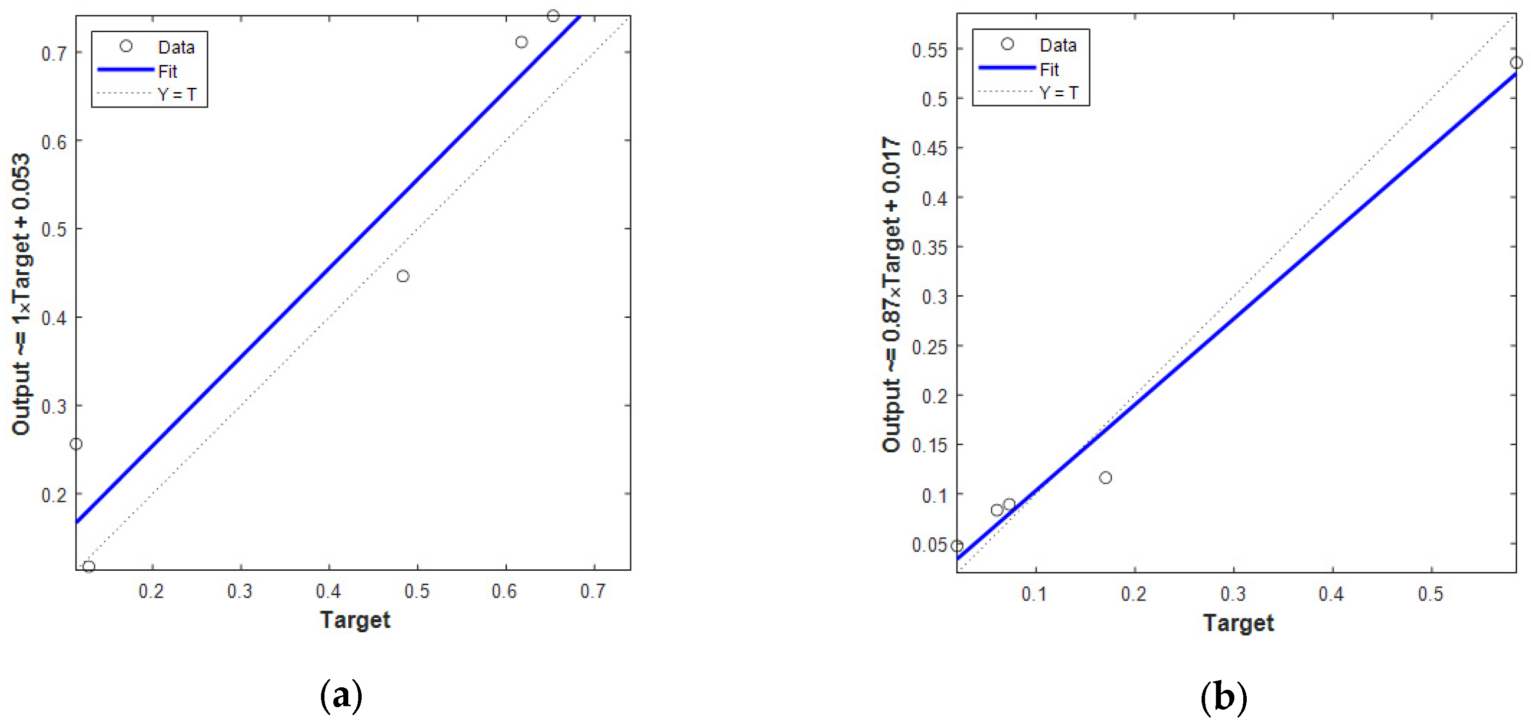
• Robust Performance on Unseen Data: The model demonstrates exceptionally high prediction accuracy on previously unseen data (e.g., R² = 0.97 for Ra, 0.93 for B5 and B8), addressing a major limitation of earlier single-model or ANN-based approaches that typically suffer from overfitting and poor generalization.
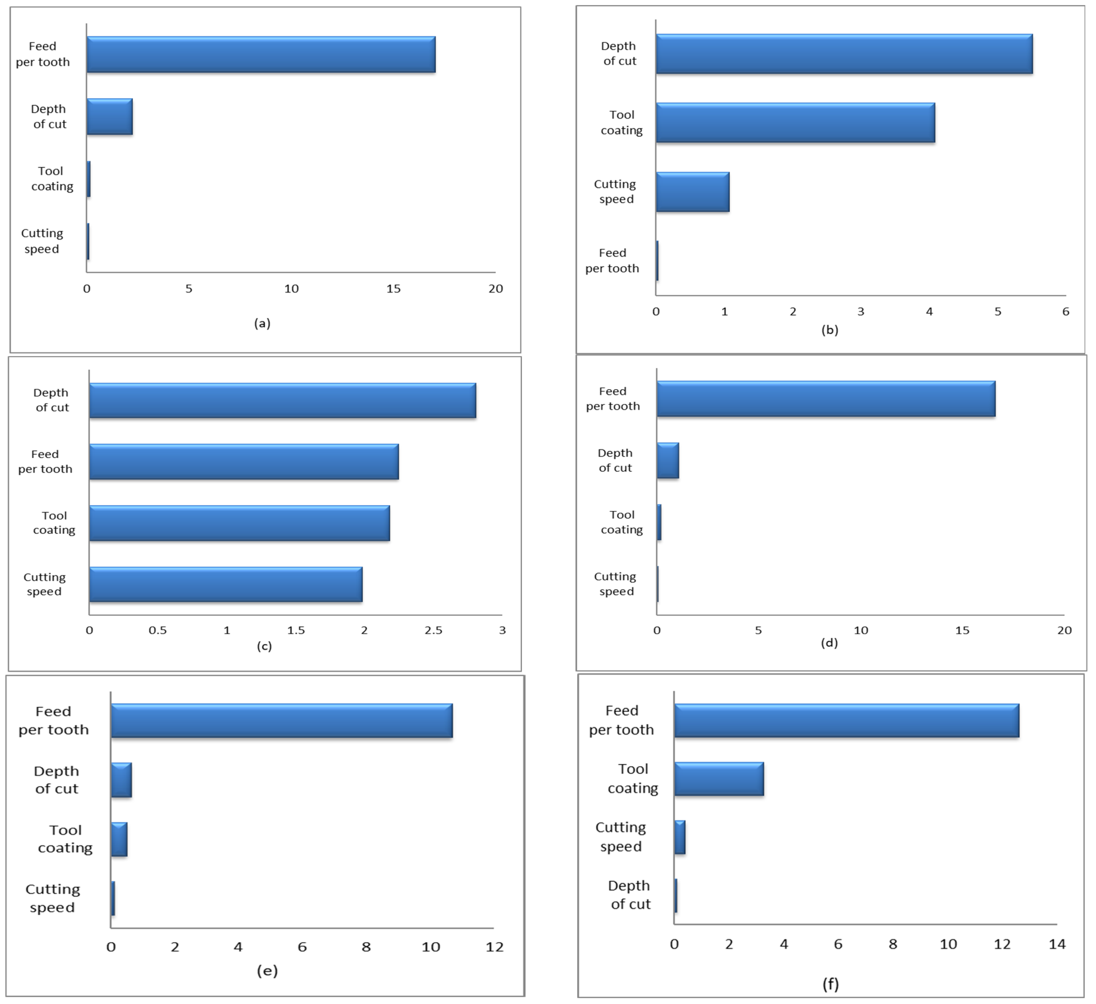
• Feature Importance Insights via the F-test: Through statistical analysis (F-test), this study identifies and ranks each output’s most influential process parameters, offering process-level insights that can guide optimization and decision-making in industrial settings.
• Experimental Validation with AA 6061: The model is trained and validated using experimentally obtained data from slot milling operations on aluminum alloy AA 6061, under a full-factorial design with controlled variables, further reinforcing the work’s practical applicability and scientific rigor.

To the authors’ knowledge, there are very few successful efforts to develop a model for predicting burr formation that achieves such high accuracy in forecasting this critical surface quality parameter, especially when compared to the results presented in this paper. It can be concluded that the size of burrs is primarily influenced by variations in feed rate, depth of cut, and cutting speed, as well as the interactions between feed and depth of cut. These factors are the dominant parameters affecting burr formation and size. This indicates that changes in these parameters significantly impact the burr formation process because of their direct effects on material removal rates and cutting forces. Milling tests that use lower values for feed per tooth and depth of cut result in thinner burrs. Additionally, the effect of cutting speed on burr size is minimal when compared to the impacts of feed per tooth and depth of cut. These findings support the presented statements in [17,29,69]. The model demonstrates high predictive accuracy, especially for Ra and B_t, indicating its potential for real-time optimization in machining operations. This reduces the necessity for extensive experimental trials and helps minimize production costs. By addressing these gaps, the proposed study makes a novel contribution to the field of precision manufacturing. It provides a scalable, interpretable, and accurate predictive model that can help manufacturers optimize cutting conditions, reduce postprocessing costs, and enhance product quality. This approach has potential for broader application in real-time process control, supporting the development of smart and sustainable manufacturing systems.

6. Conclusions

In machining processes—particularly milling—surface quality is a key determinant of part performance and production efficiency. Among the critical surface quality indicators, burr formation and surface roughness directly influence downstream operations, product reliability, and manufacturing costs. This study investigated the use of an optimized ensemble learning regression model to predict key output parameters—namely, burr dimensions (B1, B2, B4, B5, B8) and surface roughness (Ra)—in the slot milling of AA 6061 alloy. Cutting parameters were employed as model inputs, and the predictive performance was evaluated using MSE, MAE, and R² metrics.

The key findings of this study are summarized as follows:

• Surface roughness predictions achieved higher accuracy compared to burr-related predictions when tested on unseen data. This disparity suggests that burr formation is more sensitive to complex and nonlinear interactions among process parameters, making it inherently more challenging to model.
• Sensitivity analysis using the F-test revealed that the influence of input parameters varies significantly across different output responses. This finding highlights the need for customized models that focus on the most critical variables for each output, thereby improving prediction precision.
• Hyperparameter optimization was shown to significantly enhance model performance. Careful tuning of the ensemble learning model’s internal settings is essential for achieving high accuracy and generalization capability.

This study demonstrates the potential of advanced machine learning—specifically optimized ensemble regression—to model and predict critical quality indicators in milling processes. The novel application of ensemble learning to simultaneously forecast burr size and surface roughness, with robust performance on unseen data, represents a meaningful advancement in manufacturing intelligence. Moreover, the framework developed here offers valuable insight into the underlying process dynamics and can serve as a foundation for real-time control and optimization in smart manufacturing environments. Future work may explore further integrating explainable AI tools to interpret model behavior and expand the approach to other materials and machining operations for broader applicability.

References

1. Niknam, S.A.; Songmene, V. Milling burr formation, modeling and control: A review. Proc. Inst. Mech. Eng. Part B J. Eng. Manuf. 2015, 229, 893–909. [Google Scholar]
2. Gillespie, L.K. Deburring and Edge Finishing Handbook; Society of Manufacturing Engineers: Southfield, MI, USA, 1999. [Google Scholar]
3. Gillespie, L. The Battle of the Burr: New Strategies and New Tricks; Deburring Technology International, Incorporated: Mount Vernon, OH, USA, 1996; Volume 116, pp. 69–70. [Google Scholar]
4. Niknam, S.A.; Davoodi, B.; Davim, J.P. Songmene Mechanical deburring and edge-finishing processes for aluminum parts—A review. Int. J. Adv. Manuf. Technol. 2018, 95, 1101–1125. [Google Scholar]
5. Nakayama, K.; Arai, M. Burr formation in metal cutting. CIRP Ann. 1987, 36, 33–36. [Google Scholar] [CrossRef]
6. Olvera, O.; Barrow, G. An experimental study of burr formation in square shoulder face milling. Int. J. Mach. Tools Manuf. 1996, 36, 1005–1020. [Google Scholar]
7. Olvera, O.; Barrow, G. Influence of exit angle and tool nose geometry on burr formation in face milling operations. Proc. Inst. Mech. Eng. Part B J. Eng. Manuf. 1998, 212, 59–72. [Google Scholar]
8. Lin, T.-R. Experimental study of burr formation and tool chipping in the face milling of stainless steel. J. Mater. Process. Technol. 2000, 108, 12–20. [Google Scholar]
9. Avila, M.C.; Dornfeld, D.A. On the Face Milling Burr Formation Mechanisms and Minimization Strategies at High Tool Engagement; Laboratory for Manufacturing and Sustainability: Berkeley, CA, USA, 2004. [Google Scholar]
10. Korkut, I.; Donertas, M. The influence of feed rate and cutting speed on the cutting forces, surface roughness and tool–chip contact length during face milling. Mater. Des. 2007, 28, 308–312. [Google Scholar]
11. Kitajima, K. Study on mechanism and similarity of burr formation in face milling and drilling. Technol. Rep. Kansai Univ. 1990, 32, 1. [Google Scholar]
12. Hashimura, M.; Hassamontr, J.; Dornfeld, D. Effect of in-plane exit angle and rake angles on burr height and thickness in face milling operation. J. Manuf. Sci. Eng. 1999, 121, 13–19. [Google Scholar]
13. Kishimoto, W.; Miyake, T.; Yamamoto, A.; Yamanaka, K.; Takano, K. Study of burr formation in face milling. Conditions for the secondary burr formation. Bull. Jpn. Soc. Precis. Eng. 1980, 15, 51–52. [Google Scholar]
14. Chern, G.-L. Analysis of Burr Formation and Breakout in Metal Cutting. Ph.D. Thesis, University of California, Berkeley, CA, USA, 1993. [Google Scholar]
15. Aurich, J.C.; Dornfeld, D.; Arrazola, P.J.; Franke, V.; Leitz, L.; Min, S. Burrs—Analysis, control and removal. CIRP Ann. 2009, 58, 519–542. [Google Scholar] [CrossRef]
16. Lekkala, R.; Bajpai, V.; Singh, R.K.; Joshi, S.S. Characterization and modeling of burr formation in micro-end milling. Precis. Eng. 2011, 35, 625–637. [Google Scholar] [CrossRef]
17. Mian, A.; Driver, N.; Mativenga, P. Estimation of minimum chip thickness in micro-milling using acoustic emission. Proc. Inst. Mech. Eng. Part B J. Eng. Manuf. 2011, 225, 1535–1551. [Google Scholar] [CrossRef]
18. Tang, Y.; He, Z.; Lu, L.; Wang, H.; Pan, M. Burr formation in milling cross-connected microchannels with a thin slotting cutter. Precis. Eng. 2011, 35, 108–115. [Google Scholar] [CrossRef]
19. Chen, M.; Liu, G.; Shen, Z. Study on active process control of burr formation in Al-alloy milling process. In Proceedings of the 2006 IEEE International Conference on Automation Science and Engineering, Shanghai, China, 8–10 October 2006. [Google Scholar]
20. Karayel, D. Prediction and control of surface roughness in CNC lathe using artificial neural network. J. Mater. Process. Technol. 2009, 209, 3125–3137. [Google Scholar] [CrossRef]
21. Kumpati, S.N.; Kannan, P. Identification and control of dynamical systems using neural networks. IEEE Trans. Neural Netw. 1990, 1, 4–27. [Google Scholar]
22. Gupta, M.; Jin, L.; Homma, N. Static and Dynamic Neural Networks: From Fundamentals to Advanced Theory; John Wiley and Sons: Hoboken, NJ, USA, 2004. [Google Scholar]
23. Cheng, C.-T.; Wang, W.-C.; Xu, D.-M. Optimizing hydropower reservoir operation using hybrid genetic algorithm and chaos. Water Resour. Manag. 2008, 22, 895–909. [Google Scholar] [CrossRef]
24. Al Hazza, M.H.; Adesta, E.Y. Investigation of the effect of cutting speed on the Surface Roughness parameters in CNC End Milling using Artificial Neural Network. In IOP Conference Series: Materials Science and Engineering; IOP Publishing: Bristol, UK, 2013. [Google Scholar]
25. Barua, M.K.; Rao, J.S.; Anbuudayasankar, S.P.; Page, T. Measurement of surface roughness through RSM: Effect of coated carbide tool on 6061-t4 aluminium. Int. J. Enterp. Netw. Manag. 2010, 4, 136–153. [Google Scholar] [CrossRef]
26. Datta, S.; Davim, J.P. (Eds.) Machine Learning in Industry; Springer: Berlin/Heidelberg, Germany, 2022. [Google Scholar] [CrossRef]
27. Niknam, S.A.; Songmene, V. Factors governing burr formation during high-speed slot milling of wrought aluminum alloys. Proc. Inst. Mech. Eng. Part B J. Eng. Manuf. 2013, 227, 1165–1179. [Google Scholar] [CrossRef]
28. Toropov, A.; Ko, S.-L.; Lee, J. A new burr formation model for orthogonal cutting of ductile materials. CIRP Ann. 2006, 55, 55–58. [Google Scholar] [CrossRef]
29. Niknam, S.A.; Songmene, V. Modeling of burr thickness in milling of ductile materials. Int. J. Adv. Manuf. Technol. 2013, 66, 2029–2039. [Google Scholar] [CrossRef]
30. Chern, G.-L. Experimental observation and analysis of burr formation mechanisms in face milling of aluminum alloys. Int. J. Mach. Tools Manuf. 2006, 46, 1517–1525. [Google Scholar] [CrossRef]
31. Benardos, P.; Vosniakos, G.-C. Predicting surface roughness in machining: A review. Int. J. Mach. Tools Manuf. 2003, 43, 833–844. [Google Scholar] [CrossRef]
32. Kadirgama, K.; Noor, M.; Rahman, M. Optimization of surface roughness in end milling using potential support vector machine. Arab. J. Sci. Eng. 2012, 37, 2269–2275. [Google Scholar] [CrossRef]
33. Nasr, G.; Davoodi, B. Prediction of profile error in aspheric grinding of spherical fused silica by ensemble learning regression methods. Precis. Eng. 2024, 88, 65–80. [Google Scholar] [CrossRef]
34. Liu, Y.; Yao, X. Ensemble learning via negative correlation. Neural Netw. 1999, 12, 1399–1404. [Google Scholar] [CrossRef]
35. Liu, Y.; Yao, X.; Higuchi, T. Evolutionary ensembles with negative correlation learning. IEEE Trans. Evol. Comput. 2000, 4, 380–387. [Google Scholar]
36. Breiman, L. Random forests. Mach. Learn. 2001, 45, 5–32. [Google Scholar] [CrossRef]
37. Rodriguez, J.J.; Kuncheva, L.I.; Alonso, C.J. Rotation forest: A new classifier ensemble method. IEEE Trans. Pattern Anal. Mach. Intell. 2006, 28, 1619–1630. [Google Scholar] [CrossRef]
38. Lukoševičius, M.; Jaeger, H. Reservoir computing approaches to recurrent neural network training. Comput. Sci. Rev. 2009, 3, 127–149. [Google Scholar] [CrossRef]
39. Al-Anazi, A.; Gates, I. A support vector machine algorithm to classify lithofacies and model permeability in heterogeneous reservoirs. Eng. Geol. 2010, 114, 267–277. [Google Scholar] [CrossRef]
40. Ahmadi, M.A.; Soleimani, R.; Bahadori, A. A computational intelligence scheme for prediction equilibrium water dew point of natural gas in TEG dehydration systems. Fuel 2014, 137, 145–154. [Google Scholar] [CrossRef]
41. Yu, H.; Rezaee, R.; Wang, Z.; Han, T.; Zhang, Y.; Arif, M.; Johnson, L. A new method for TOC estimation in tight shale gas reservoirs. Int. J. Coal Geol. 2017, 179, 269–277. [Google Scholar] [CrossRef]
42. Yu, H.; Wang, Z.; Rezaee, R.; Liu, X.; Zhang, Y.; Imokhe, O. Fluid type identification in carbonate reservoir using advanced statistical analysis. In Proceedings of the SPE Oil and Gas India Conference and Exhibition, Mumbai, India, 4–6 April 2017. [Google Scholar]
43. Lee, C.; Lee, G.G. Information gain and divergence-based feature selection for machine learning-based text categorization. Inf. Process. Manag. 2006, 42, 155–165. [Google Scholar] [CrossRef]
44. Dai, J.; Xu, Q. Attribute selection based on information gain ratio in fuzzy rough set theory with application to tumor classification. Appl. Soft Comput. 2013, 13, 211–221. [Google Scholar] [CrossRef]
45. Yitzhaki, S. Relative deprivation and the Gini coefficient. Q. J. Econ. 1979, 93, 321–324. [Google Scholar] [CrossRef]
46. Tahraoui, H.; Amrane, A.; Belhadj, A.-E.; Zhang, J. Modeling the organic matter of water using the decision tree coupled with bootstrap aggregated and least-squares boosting. Environ. Technol. Innov. 2022, 27, 102419. [Google Scholar] [CrossRef]
47. Zheng, Z. Boosting and Bagging of Neural Networks with Applications to Financial Time Series; The University of Chicago: Chicago, IL, USA, 2006. [Google Scholar]
48. Galar, M.; Fernández, A.; Barrenechea, E.; Sola, H.B. Dynamic classifier selection for one-vs-one strategy: Avoiding non-competent classifiers. Pattern Recognit. 2013, 46, 3412–3424. [Google Scholar] [CrossRef]
49. Bauer, E.; Kohavi, R. An empirical comparison of voting classification algorithms: Bagging, boosting, and variants. Mach. Learn. 1999, 36, 105–139. [Google Scholar] [CrossRef]
50. Mendes-Moreira, J.; Soares, C.; Jorge, A.M.; De Sousa, J.F. Ensemble approaches for regression: A survey. ACM Comput. Surv. 2012, 45, 1–40. [Google Scholar] [CrossRef]
51. Unger, D.A.; van den Dool, H.; O’Lenic, E.; Collins, D. Ensemble Regression. Mon. Weather. Rev. 2009, 137, 2365–2379. [Google Scholar] [CrossRef]
52. Breiman, L. Bagging predictors. Mach. Learn. 1996, 24, 123–140. [Google Scholar] [CrossRef]
53. Hastie, T.; Tibshirani, R.; Friedman, J. The Elements of Statistical Learning: Data Mining, Inference, and Prediction; Springer: Berlin/Heidelberg, Germany, 2009; Volume 2. [Google Scholar]
54. Inoue, A.; Kilian, L. How useful is bagging in forecasting economic time series? A case study of US consumer price inflation. J. Am. Stat. Assoc. 2008, 103, 511–522. [Google Scholar] [CrossRef]
55. Zhang, J. Developing robust non-linear models through bootstrap aggregated neural networks. Neurocomputing 1999, 25, 93–113. [Google Scholar] [CrossRef]
56. Friedman, J.H. Greedy function approximation: A gradient boosting machine. Ann. Stat. 2001, 29, 1189–1232. [Google Scholar] [CrossRef]
57. Ashqar, H.I.; Elhenawy, M.; Rakha, H.A.; Almannaa, M.; House, L. Network and station-level bike-sharing system prediction: A San Francisco bay area case study. J. Intell. Transp. Syst. 2022, 26, 602–612. [Google Scholar] [CrossRef]
58. Zhang, Y.; Xu, X. Predictions of the total crack length in solidification cracking through LSBoost. Metall. Mater. Trans. A 2021, 52, 985–1005. [Google Scholar] [CrossRef]
59. Barutçuoğlu, Z.; Alpaydın, E. A comparison of model aggregation methods for regression. In International Conference on Artificial Neural Networks; Springer: Berlin/Heidelberg, Germany, 2003. [Google Scholar]
60. Belsley, D.A.; Kuh, E.; Welsch, R.E. Regression Diagnostics: Identifying Influential Data and Sources of Collinearity; John Wiley and Sons: Hoboken, NJ, USA, 2005. [Google Scholar]
61. Hong, S.H.; Lee, M.W.; Lee, D.S.; Park, J.M. Monitoring of sequencing batch reactor for nitrogen and phosphorus removal using neural networks. Biochem. Eng. J. 2007, 35, 365–370. [Google Scholar] [CrossRef]
62. Bousselma, A.; Abdessemed, D.; Tahraoui, H.; Amrane, A. Artificial intelligence and mathematical modelling of the drying kinetics of pre-treated whole apricots. Kem. U Ind. 2021, 70, 651–667. [Google Scholar] [CrossRef]
63. Dolling, O.R.; Varas, E.A. Artificial neural networks for streamflow prediction. J. Hydraul. Res. 2002, 40, 547–554. [Google Scholar] [CrossRef]
64. Manssouri, I.; Manssouri, M.; El Kihel, B. Fault detection by K-NN algorithm and MLP neural networks in a distillation column: Comparative study. J. Inf. Intell. Knowl. 2011, 3, 201. [Google Scholar]
65. Manssouri, I.; El Hmaidi, A.; Manssouri, T.E.; El Moumni, B. Prediction levels of heavy metals (Zn, Cu and Mn) in current Holocene deposits of the eastern part of the Mediterranean Moroccan margin (Alboran Sea). IOSR J. Comput. Eng. 2014, 16, 117–123. [Google Scholar] [CrossRef]
66. ASM International. ASM Handbook: Metallography and Microstructures; ASM International: Almere, The Netherlands, 2004. [Google Scholar]
67. Davim, J.P. Machining: A bibliometric analysis. Int. J. Mach. Mach. Mater. 2024, 26, 293–295. [Google Scholar]
68. Fang, N.; Pai, P.S.; Edwards, N. Neural network modeling and prediction of surface roughness in machining aluminum alloys. J. Comput. Commun. 2016, 4, 1–9. [Google Scholar] [CrossRef]
69. Lauderbaugh, L.K. Analysis of the effects of process parameters on exit burrs in drilling using a combined simulation and experimental approach. J. Mater. Process. Technol. 2009, 209, 1909–1919. [Google Scholar] [CrossRef]
Figure 1. Slot milling burrs (adapted from [19]).
Machines 13 00494 g001
Figure 2. Ensemble learner flowchart [33].
Machines 13 00494 g002
Figure 3. Comparison charts representing the experimental data and prediction data for (a) B1 and (b) Ra.
Machines 13 00494 g003
Figure 4. Regression analysis comparing test data and prediction model output for (a) B1 and (b) Ra.
Machines 13 00494 g004
Figure 5. The importance level of each feature sorted using the F-test algorithm. F-test of (a) B1, (b) B2, (c) B4, (d) B5, (e) B8, and (f) Ra.
Machines 13 00494 g005