Fault Detection in Gearboxes Using Fisher Criterion and Adaptive Neuro-Fuzzy Inference

Abstract

Gearboxes are autonomous devices essential for power transmission in various mechanical systems. When a failure occurs, it can lead to an inability to perform the required functions, potentially resulting in a complete shutdown of the mechanism and causing significant operational disruptions. Consequently, deploying expert methods for fault detection and diagnosis is crucial to ensuring the reliability and efficiency of these systems. Artificial intelligence (AI) techniques show promise for fault diagnosis, but their accuracy can be hindered by noise and manufacturing imperfections that distort mechanical signatures. Thorough data analysis and preprocessing are vital to preserving these critical features. Validating approaches through numerical simulations before experimentation is essential to identify model limitations and minimize risks. A hybrid approach, combining AI and physics-based models, could provide a robust solution by leveraging the strengths of both domains: AI for its ability to process large volumes of data and physics-based models for their reliability in modeling complex mechanical behaviors. This paper proposes a comprehensive diagnostic methodology. It starts with feature extraction from time-domain analysis, which helps identify critical indicators of gearbox performance. Following this, a feature selection process is applied using the Fisher criterion, which ensures that only the most relevant features are retained for further analysis. These selected features are then employed to train an Adaptive Neuro-Fuzzy Inference System (ANFIS), a sophisticated approach that combines the learning capabilities of neural networks with the reasoning abilities of fuzzy logic. The proposed methodology is evaluated using a dataset of gear faults generated through energy simulations based on a six-degree-of-freedom (6-DOF) model, followed by a secondary validation on an experimental dataset.

1. Introduction

Monitoring rotating machinery is a critical task in many industries, as it directly impacts operational safety and productivity. The primary objectives are to ensure operator safety and prevent unexpected production shutdowns, which can lead to significant financial losses. Reliability studies on industrial systems have shown that gearboxes are a critical component due to their high failure rates and the severe damage they can cause [1]. Gears can be affected by over 20 types of faults, as classified by ISO 10825 [2], which fall into six main categories: surface fatigue, surface deterioration, scuffing, deformation, cracking, and tooth breakage [3]. The first four faults are considered surface-related wear issues. They can be caused by various factors, such as poor lubrication, contaminated lubricants, or misaligned gear mounting, which accelerates surface degradation through direct contact or abrasive wear. Repeated shocks during startup and shutdown can also lead to surface fatigue and permanent deformation. These faults can be mitigated by adhering to proper lubricant change intervals, selecting the right lubricant, using alignment measurement tools, and installing flexible couplings to reduce gear surface impacts. Cracking and tooth breakage are sudden, catastrophic failures that can result from the same factors, along with advanced corrosion (which can initiate cracks) and poor design that fails to account for stress concentration points. Preventive measures include ultrasonic inspections and preliminary stress concentration analysis to minimize their effects [3,4]. To detect these faults, robust and effective strategies for fault detection and diagnosis are essential [5]. There are two main approaches to fault detection and diagnosis: model-based and data-driven. The model-based approach involves creating mathematical models of the physical phenomena involved in machinery operation and solving these models to predict faults. In contrast, the data-driven approach focuses on collecting and analyzing operational data to identify signs of degradation or the presence of faults [6]. This analysis typically includes feature extraction from time-domain signals, where statistical indicators such as root mean square (RMS), skewness, and kurtosis are calculated. Advanced algorithms are commonly employed to select the most discriminative features, with popular approaches including principal component analysis (PCA) and Fisher’s criterion [7]. While Fisher’s method can be limited when handling highly complex datasets, it offers the advantage of supervised separation, making it particularly well suited for fault diagnosis applications compared to PCA. Fisher focuses on selecting features by maximizing the inter-class distance and minimizing the intra-class distance, whereas PCA constructs new features by combining the original ones based on the direction of maximum variance. When working with statistical indicators, it is generally preferable to retain the original features to ensure better interpretability [8].

Recently, several studies have adopted the Fisher score for discriminative feature selection to enhance inter-class separation [9]. Sun et al. [10] proposed a fault diagnosis method for railway point machines based on vibration signals. They combined feature extraction using variational mode decomposition and dispersion entropy with a two-stage feature selection method involving Fisher’s criterion and ReliefF. This approach achieved effective class discrimination with high accuracy. Kumar et al. [11] developed an efficient method for diagnosing bearing defects in rotating machines using vibration signal analysis. Their Automated Fault Investigation approach combines Fisher score and genetic algorithm for feature selection with a hyperparameter-tuned Support Vector Machine classifier. This method achieves high classification accuracy for defects in rolling element bearings, including inner race, outer race, and combined faults. The study demonstrates that feature selection significantly enhances model performance while reducing computational time. Ardali et al. [12] demonstrated the relevance of the Fisher discriminant ratio (FDR) in their study by comparing it with other feature selection methods. The FDR was used to assess the effectiveness of the feature subsets selected by the genetic algorithm and eXtreme Gradient Boosting (XGBoost). The results showed that FDR provided effective class discrimination, enhancing the performance of the fault diagnosis model. This method proved particularly useful in improving the accuracy of fault detection and diagnosis in chemical processes by optimizing the separation between different fault classes. Liu et al. [13] addressed the challenges of unobserved faults in data-based semi-supervised industrial fault classification by proposing a robust semi-supervised Fisher discriminant analysis model. To tackle this, a sample recognition technique was developed to preprocess training samples and identify unobserved fault samples. Additionally, a regularized between-class was constructed to fully utilize both supervised and unsupervised information, enhancing classification accuracy. The proposed model was shown to be effective in experiments on the Tennessee Eastman process and a real industrial air separation unit, demonstrating its superiority in addressing both offline and online fault classification challenges.

The feature selection step is always followed by classification to ensure fault detection and diagnosis. Given the nature of the data, which consist of a feature vector, an efficient machine learning approach is required. The Adaptive Neuro-Fuzzy Inference System (ANFIS) combines fuzzy logic and neural networks, specifically designed to learn from nonlinear and complex data. Zemali et al. [14] proposed a method integrating ANFIS models and Kalman observers to detect and isolate faults in wind turbines. This approach enables early and precise fault identification, improving wind turbine availability despite varying environmental conditions. Akbari et al. [15] demonstrated the effectiveness of the ANFIS for fault detection, classification, and location, emphasizing its independence from wave propagation characteristics. The study optimized the ANFIS model using Harris hawks optimization and cuckoo search algorithms, comparing their performance with traditional training methods. Principal component analysis and discrete wavelet transform were employed to extract relevant features for training and testing the ANFIS model. The results showed that the optimized ANFIS achieved superior fault classification and location accuracy, outperforming traditional traveling wave models. Kanwal et al. [16] compared ANFIS with other fault detection and localization methods for transmission lines, demonstrating that ANFIS outperformed traditional techniques like traveling wave and impedance-based methods. Using the IEEE 9-bus system for simulations, ANFIS models achieved superior accuracy in fault classification, detection, and localization. The ANFIS-based model had lower error rates compared to backpropagation, self-organizing maps, and the hybrid discrete wavelet–ANFIS model, making it a promising choice for real-time protection systems in power networks. Perez et al. [17] proposed a robust fault diagnosis methodology for wind turbines based on zonotopic state estimators using Takagi–Sugeno models. The approach utilizes a Multiple Output ANFIS, which allows for multi-output architecture, reducing training time, uncertainties, and model complexity. This method improves fault detection by adjusting the parameters of the zonotopic estimator to account for modeling uncertainties. The approach was validated using a certified wind turbine case study, contributing to enhanced safety and operability of wind turbines through improved diagnostic systems.

The mentioned studies have relied on experimental datasets to validate the proposed methodologies. However, these datasets may contain acquisition noise and interference from other faults, which could compromise the accuracy and reliability of the methodologies. Furthermore, while this approach is specifically designed for fault classification and signature identification, it must first demonstrate its effectiveness in these tasks before being applied to experimental data, as demonstrated by [18] for the diagnosis of tooth root cracks. In our study, we tested the methodology on multiple faults to ensure robustness in such environments, which is crucial for the successful deployment of these methods in real-world applications.

The framework presented in this paper introduces an intelligent methodology for gearbox fault detection and diagnosis. The contributions presented in this work are as follows:

• A six-degree-of-freedom (6-DOF) multi-body dynamic model was developed to represent the transmission system and various fault conditions.
• Features were extracted from time-domain signal analysis, with feature selection performed based on Fisher’s criterion.
• Fault classification was carried out using an Adaptive Neuro-Fuzzy Inference System (ANFIS) to facilitate automation and real-time application.
• The proposed diagnostic methodology was experimentally validated to demonstrate its reliability and effectiveness.

The paper is organized into five sections. Section 1 introduces the problem and provides the state of the art in recent frameworks. Section 2 covers the energetic modeling of gear transmission in both healthy and faulty states. Section 3 presents time meshing stiffness as well as the vibrational response of the previous cases. Section 4 discusses the methodology for feature extraction, selection, and learning. Section 5 concludes the paper and offers perspectives.

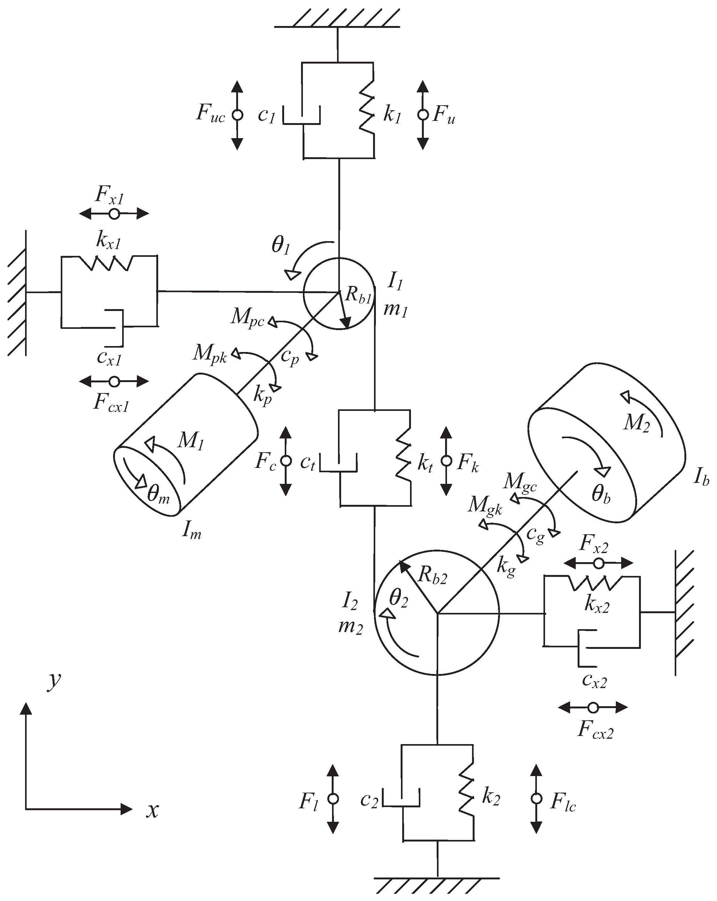
2. Gear Mesh Stiffness Modeling

The energetic modeling of gear transmission is based on calculating the energy stored in the tooth during contact between the gears. The different geometric parameters used are illustrated in Figure 1.

Figure 1 shows a gear with base radius $R_b$ featuring a single tooth to illustrate the key parameters, where the contact force F between mating teeth is inclined at angle ${\alpha }_1$ from the vertical line along the line of action, resolving into orthogonal components $F_a$ and $F_b$ along the x and y axes, respectively. The contact point is located at height d from the tooth root and distance h from the tooth centerline, while each point along the tooth profile is characterized by angle $\alpha$ (where ${\alpha }_2$ specifically denotes the root angle), height x ranging from zero to the full tooth height, and radial distance $h_x$ with $h_r$ at the tooth tip [20].

The energies considered in this model are Hertzian, bending, axial compressive, and shear energy. From these energies, the transmission rigidities $k_h$, $k_b$, $k_a$, and $k_s$ are derived and formulated as follows [19].

$$k_h=\frac{\pi EL}{4(1-{\nu }^2)}$$

(1)

$$\frac{1}{k_b}={\int }_{-{\alpha }_1}^{{\alpha }_2}\frac{3{[1+cos{\alpha }_1(({\alpha }_2-\alpha )sin\alpha -cos\alpha )]}^2({\alpha }_2-\alpha )cos\alpha }{2EL{\left(({\alpha }_2-\alpha )cos\alpha +sin\alpha \right)}^3}d\alpha$$

(2)

$$\frac{1}{k_a}={\int }_{-{\alpha }_1}^{{\alpha }_2}\frac{({\alpha }_2-\alpha )cos\alpha {sin}^2{\alpha }_1}{2EL\left(({\alpha }_2-\alpha )cos\alpha +sin\alpha \right)}d\alpha$$

(3)

$$\frac{1}{k_s}={\int }_{-{\alpha }_1}^{{\alpha }_2}\frac{1.2(1+\nu )({\alpha }_2-\alpha )cos\alpha {cos}^2{\alpha }_1}{EL\left(({\alpha }_2-\alpha )cos\alpha +sin\alpha \right)}d\alpha$$

(4)

where E, L, and $\nu$ denote Young’s modulus, tooth width, and Poisson’s ratio, respectively.

The expression for the effective total rigidity $k_t$ of a single pair of teeth is formulated as in Equation (5), where indices 1 and 2 represent the pinion and the gear, respectively.

$$k_t=\frac{1}{\frac{1}{k_h}+\frac{1}{k_{b1}}+\frac{1}{k_{a1}}+\frac{1}{k_{s1}}+\frac{1}{k_{b2}}+\frac{1}{k_{a2}}+\frac{1}{k_{s2}}}$$

(5)

For the engagement duration of two pairs of teeth, the effective total rigidity of engagement is the sum of the rigidities of the two pairs, as given by Equation (6).

$$k_t=\sum _{i=1}^2\left(\frac{1}{\frac{1}{k_{h,i}}+\frac{1}{k_{b1,i}}+\frac{1}{k_{a1,i}}+\frac{1}{k_{s1,i}}+\frac{1}{k_{b2,i}}+\frac{1}{k_{a2,i}}+\frac{1}{k_{s2,i}}}\right)$$

(6)

where $i=1$ corresponds to the first pair of teeth in contact when there are two pairs engaged, and $i=2$ corresponds to the second pair. Equations (1)–(6) are reproduced from [19,20].

For the modeling of the following faults, it is assumed that the defect affects the pinion teeth with a base circle radius denoted as $R_{b1}$.

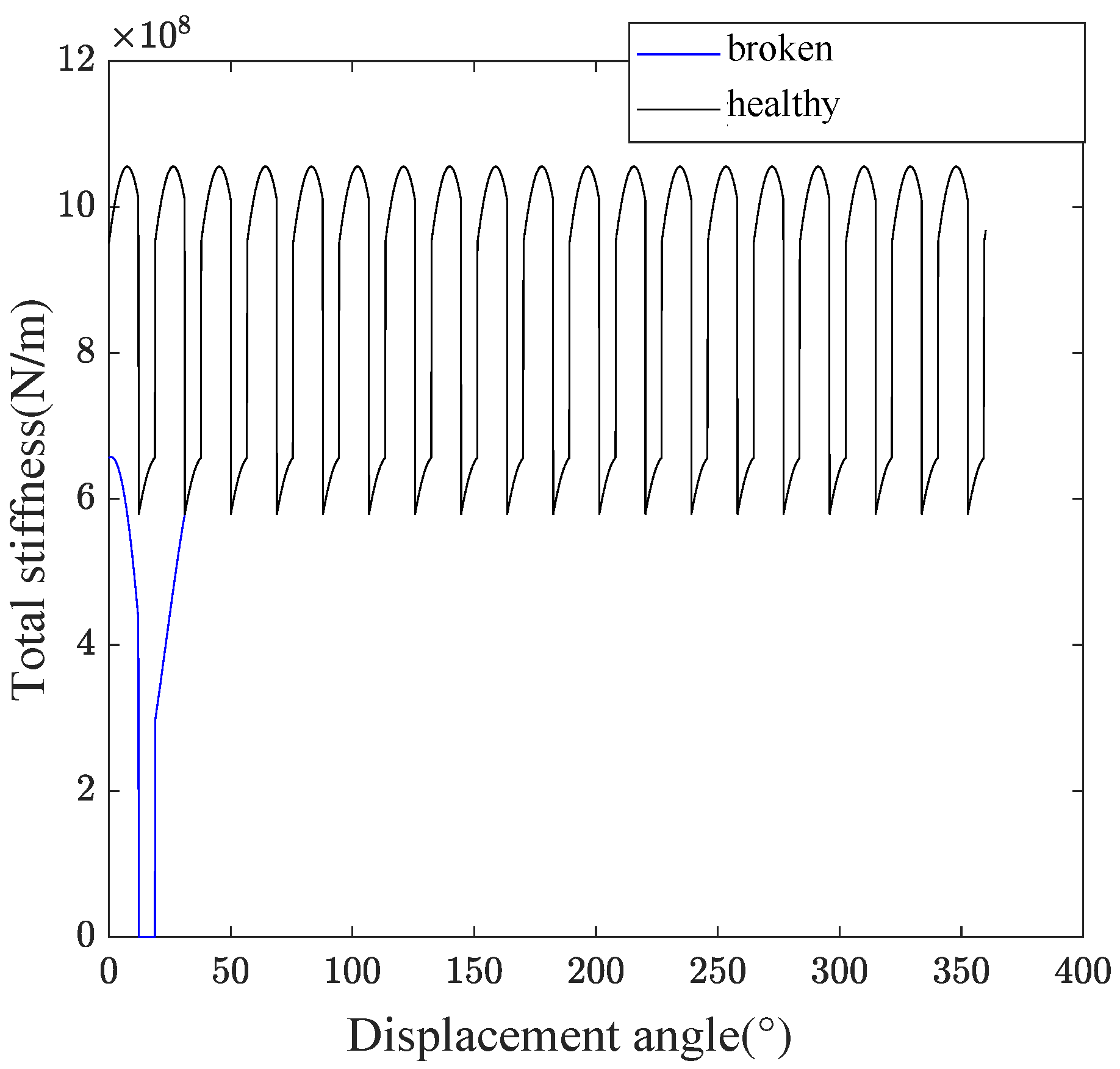
2.1. Broken Tooth Fault Modeling

The deterioration of a tooth, as illustrated in Figure 2, shows the meshing of two gears with a missing tooth represented by dotted lines. This reduces the rigidity of the gear system because a broken tooth can no longer engage properly with its counterpart. Typically, two pairs of teeth are in contact simultaneously; however, with a broken tooth, only one pair will be in contact during the same period. This halves the total rigidity of the gear. Therefore, the new formulation for the total rigidity noted $k_{t_{\mathrm{broken}}}$ is reproduced from [20] as follows.

$$k_{t_{\mathrm{broken}}}=\frac{1}{\frac{1}{k_{h,1}}+\frac{1}{k_{b1,1}}+\frac{1}{k_{s1,1}}+\frac{1}{k_{a1,1}}+\frac{1}{k_{b2,1}}+\frac{1}{k_{s2,1}}+\frac{1}{k_{a2,1}}}$$

(7)

2.2. Crack Tooth Fault Modeling

The gear tooth crack illustrated in Figure 3 typically starts at the point of greatest stress and develops at the tooth root. Furthermore, the crack follows a straight path with an intersection angle $\mu$ between the crack and the central line of the tooth fixed at a constant value of 45° [20].

The crack tip with length q is located at point G positioned at coordinates ($g_c$, $h_c$) along the x and y axes, with an orientation angle ${\alpha }_g$. This crack induces a change in the moment of inertia $I_x$ and the effective cross-sectional area $A_x$ at a distance x from the tooth root. These two parameters are reproduced from [19] and formulated as follows.

$$I_x=\left\{\begin{array}{cc}\frac{1}{12}{(h_x+h_c)}^{3}L\hfill & \mathrm{if}x<g_c\hfill \\ \frac{1}{12}{\left(2h_x\right)}^{3}L\hfill & \mathrm{if}x>g_c\hfill \end{array}\right.$$

(8)

Before the crack ($x<g_c$): the moment of inertia is calculated using a height increased by the vertical position of the crack $h_x+h_c$. After the crack ($x>g_c$): the crack divides the height, and only $2h_x$ is considered.

$$A_x=\left\{\begin{array}{cc}(h_x+h_c)L\hfill & \mathrm{if}x<g_c\hfill \\ 2\left(h_x\right)L\hfill & \mathrm{if}x>g_c\hfill \end{array}\right.$$

(9)

Before the crack ($x<g_c$): the effective cross-sectional area is larger because it includes the portion up to the crack position. After the crack ($x>g_c$): the area is reduced and depends only on $2h_x$.

The expressions of distances $h_x$ and $h_c$ are formulated as in Equations (10) and (11), reproduced from [20].

$$h_x=R_{b1}\left((\alpha +{\alpha }_2)cos\alpha -sin\alpha \right)$$

(10)

$$h_c=R_{b1}sin{\alpha }_2-qsin\mu$$

(11)

The equations are incorporated into the energy expressions, and the rigidity equations reproduced from [19] are presented as follows.

$$\begin{array}{c}\hfill \frac{1}{k_b}={\int }_{-{\alpha }_1}^{-{\alpha }_g}\frac{3{[1+cos{\alpha }_1(({\alpha }_2-\alpha )sin\alpha -cos\alpha )]}^2({\alpha }_2-\alpha )cos\alpha }{2EL{\left(({\alpha }_2-\alpha )cos\alpha +sin\alpha \right)}^3}d\alpha +\\ \hfill {\int }_{-{\alpha }_g}^{{\alpha }_2}\frac{12{[1+cos{\alpha }_1(({\alpha }_2-\alpha )sin\alpha -cos\alpha )]}^2({\alpha }_2-\alpha )cos\alpha }{EL{\left(sin{\alpha }_2+({\alpha }_2-\alpha )cos\alpha -\frac{q}{R_{b1}}sin\mu +sin\alpha \right)}^3}d\alpha \end{array}$$

(12)

$$\begin{array}{c}\hfill \frac{1}{k_a}={\int }_{-{\alpha }_1}^{-{\alpha }_g}\frac{({\alpha }_2-\alpha )cos\alpha {sin}^2{\alpha }_1}{2EL\left(({\alpha }_2-\alpha )cos\alpha +sin\alpha \right)}d\alpha +\\ \hfill {\int }_{-{\alpha }_g}^{{\alpha }_2}\frac{({\alpha }_2-\alpha )cos\alpha {sin}^2{\alpha }_1}{2EL\left(sin{\alpha }_2+({\alpha }_2-\alpha )cos\alpha -\frac{q}{R_{b1}}sin\mu +sin\alpha \right)}d\alpha \end{array}$$

(13)

$$\begin{array}{c}\hfill \frac{1}{k_s}={\int }_{-{\alpha }_1}^{-{\alpha }_g}\frac{1.2(1+\nu )({\alpha }_2-\alpha )cos\alpha {cos}^2{\alpha }_1}{EL\left(({\alpha }_2-\alpha )cos\alpha +sin\alpha \right)}d\alpha +\\ \hfill {\int }_{-{\alpha }_g}^{{\alpha }_2}\frac{2.4(1+\nu )({\alpha }_2-\alpha )cos\alpha {cos}^2{\alpha }_1}{EL\left(sin{\alpha }_2+({\alpha }_2-\alpha )cos\alpha -\frac{q}{R_{b1}}sin\mu +sin\alpha \right)}d\alpha \end{array}$$

(14)

where $k_h$ and $k_a$ are calculated as in the healthy state, formulated in Equations (1) and (3), respectively.

2.3. Chipped Tooth Fault Modeling

Chipped tooth fault is a type of fault where a portion of the material detaches near the end of the tooth. In this study, assuming that the fracture occurs along the width of the tooth, meaning that the variation occurs in two directions. For this purpose, the fracture surface is represented by a triangle with dimensions b and z (see Figure 4). Assuming that the fracture is very thin compared to the tooth thickness, changes in the tooth thickness due to this chipping can be neglected when evaluating bending, shear, and axial compressive stiffnesses. As a result of integrating the calculations for these three stiffnesses, the variations caused by the failure can be disregarded, allowing these stiffnesses to be considered similar to those of a perfect tooth [21].

The chipped portion of the tooth is characterized by height measurement $d_c$ along its vertical profile, with reference to $d_h$, which represents the full height of the intact tooth structure. However, the Hertzian contact stiffness remains constant for a perfect tooth but varies proportionally in the case of a chipped tooth, due to changes in the width of the effective working surface along the tooth curve. The Hertzian contact stiffness for a chipped tooth noted $k_{h_{\mathrm{chipped}}}$ is reproduced from [21] and calculated as follows.

$$k_{h_{\mathrm{chipped}}}=\frac{\pi E{L}_c}{4(1-{\nu }^2)}$$

(15)

where $L_c$ represents the effective width of the broken tooth, which decreases where it is chipped and remains equal to the ideal length L when undamaged. This expression can be written as follows.

$$L_c=\left\{\begin{array}{cc}L\hfill & \mathrm{if}0<d_c<d_h-b\hfill \\ (\frac{d_h^{2}z}{b}-d_{h}z)\frac{1}{d_c}+L-\frac{d_{h}z}{b}\hfill & \mathrm{if}{d}_h-b<d_c<d_h\hfill \end{array}\right.$$

(16)

where $d_h$ is the height of the tooth and $d_c$ is the contact height as shown in Figure 4. The total rigidity of the pinion in the case of a chipped tooth fault can be expressed as follows.

$$k_{t_{\mathrm{chipped}}}=\frac{1}{\frac{1}{k_{h_{\mathrm{chipped}}}}+\frac{1}{k_{b_1}}+\frac{1}{k_{a1}}+\frac{1}{k_{s1}}+\frac{1}{k_{b2}}+\frac{1}{k_{a2}}+\frac{1}{k_{s2}}}$$

(17)

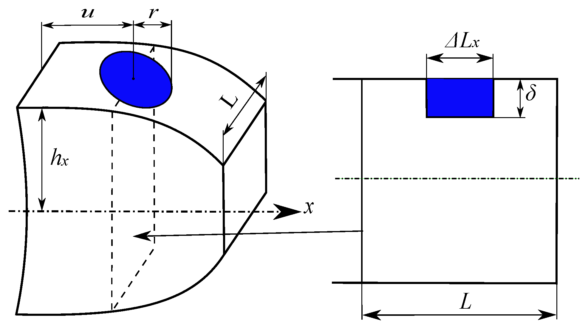
2.4. Pitting Tooth Fault Modeling

Consider the case of pitting illustrated in Figure 5, in the form of standardized holes with a radius r and a depth $\delta$, positioned at a height u from the tooth root.

Adjust the expressions for the second moment of area $I_x$ and the cross-sectional area $A_x$, and contact width $L_x$. It is necessary to introduce $\Delta I_x$, $\Delta A_x$, and $\Delta L_x$ to represent the variation in these parameters with the distance x along the line of action. The specific expressions for a tooth with a single pit are given in [22].

$$\Delta L_x=\left\{\begin{array}{cc}2\sqrt{r^2-{(u-x)}^2}\hfill & \mathrm{if}x\in [u-r,u+r]\hfill \\ 0\hfill & \mathrm{else}\hfill \end{array}\right.$$

(18)

$$\Delta A_x=\left\{\begin{array}{cc}\Delta L_x\delta \hfill & \mathrm{if}x\in [u-r,u+r]\hfill \\ 0\hfill & \mathrm{else}\hfill \end{array}\right.$$

(19)

$$\Delta I_x=\left\{\begin{array}{cc}\frac{1}{12}\Delta L_x{\delta }^3+\frac{A_x\Delta A_x{(h_x-\delta /2)}^2}{A_x-\Delta A_x}\hfill & \mathrm{if}x\in [u-r,u+r]\hfill \\ 0\hfill & \mathrm{else}\hfill \end{array}\right.$$

(20)

The modified expressions for the moment of inertia $I_x^{\prime }$, cross-sectional area $A_x^{\prime }$, and width $L_x^{\prime }$ as a function of x such that

$$\left\{\begin{array}{cc}{L}_x^{\prime }\hfill & =L_x-\Delta L_x\hfill \\ A_x^{\prime }\hfill & =A_x-\Delta A_x\hfill \\ I_x^{\prime }\hfill & =I_x-\Delta I_x\hfill \end{array}\right.$$

(21)

where $I_x$, $A_x$, and $L_x$ represent the nominal (undamaged) properties of the section. These equations mathematically capture how a circular defect of radius r centered at position u affects the geometric properties of the structural element along its length. The variation is localized to the interval $x\in \left[u-r,u+r\right]$, outside of which the properties remain unchanged from their nominal values. The parameter $\delta$ represents the depth of the defect, and $h_x$ denotes the distance from the centroidal axis to the extreme fiber at position x.

By incorporating the expressions into the energy equations, the new formulations for the rigidities are as follows.

$$k_h=\frac{\pi E(L-\Delta L_x)}{4(1-{\nu }^2)}$$

(22)

$$\frac{1}{k_b}={\int }_{-{\alpha }_1}^{{\alpha }_2}\frac{3{[1+cos{\alpha }_1(({\alpha }_2-\alpha )sin\alpha -cos\alpha )]}^2({\alpha }_2-\alpha )cos\alpha }{E(2L{\left(({\alpha }_2-\alpha )cos\alpha +sin\alpha \right)}^3-3\frac{\Delta I_x}{R_{b1}^3})}d\alpha$$

(23)

$$\frac{1}{k_a}={\int }_{-{\alpha }_1}^{{\alpha }_2}\frac{({\alpha }_2-\alpha )cos\alpha {sin}^2{\alpha }_1}{E(2L\left(({\alpha }_2-\alpha )cos\alpha +sin\alpha \right)-\frac{\Delta A_x}{R_{b1}})}d\alpha$$

(24)

$$\frac{1}{k_s}={\int }_{-{\alpha }_1}^{{\alpha }_2}\frac{1.2(1+\nu )({\alpha }_2-\alpha )cos\alpha {cos}^2{\alpha }_1}{E(L\left(({\alpha }_2-\alpha )cos\alpha +sin\alpha \right)-\frac{\Delta A_x}{2R_{b1}})}d\alpha$$

(25)

Equations (22)–(25) are reproduced from [22] and adapted to the type of teeth studied.

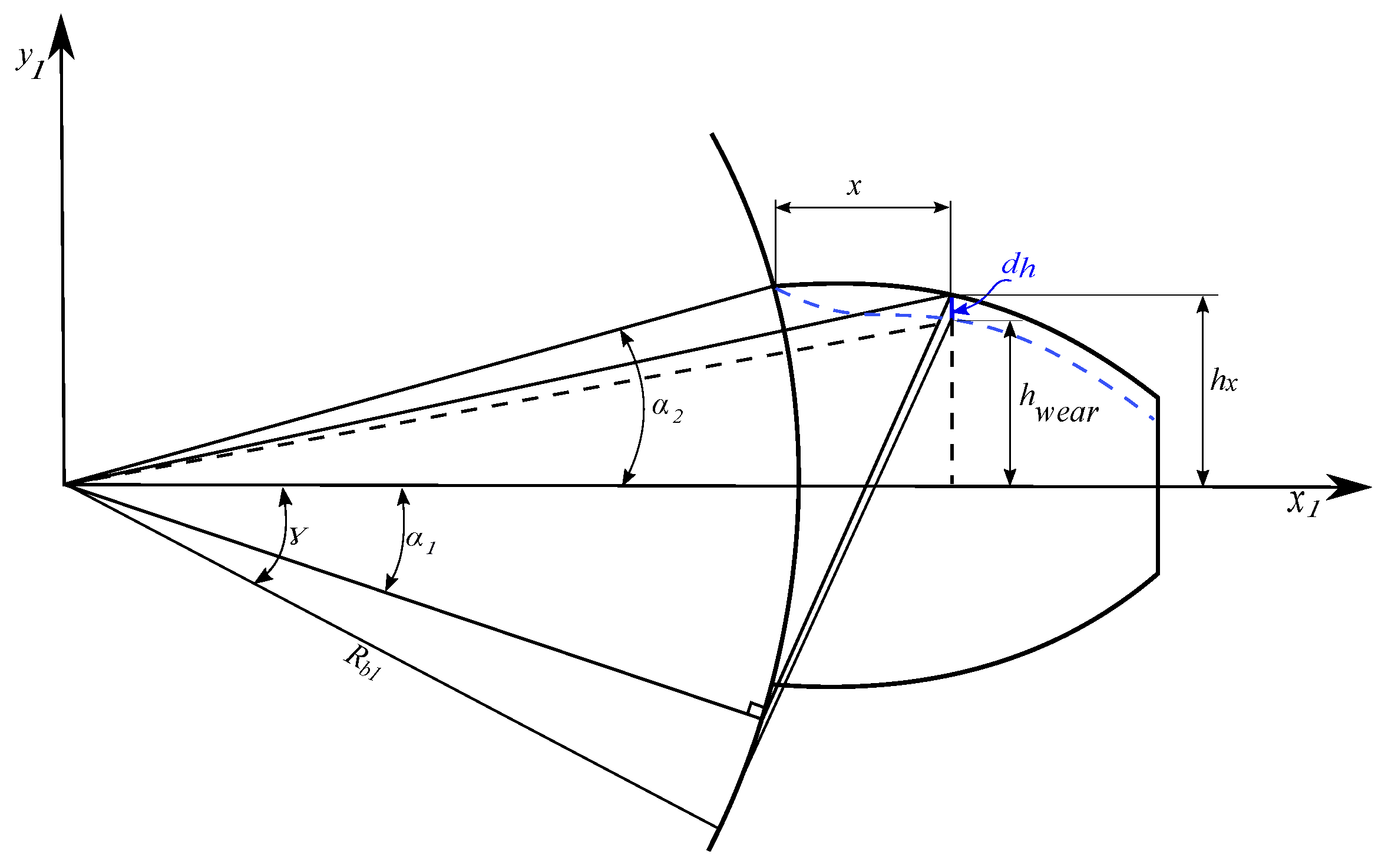
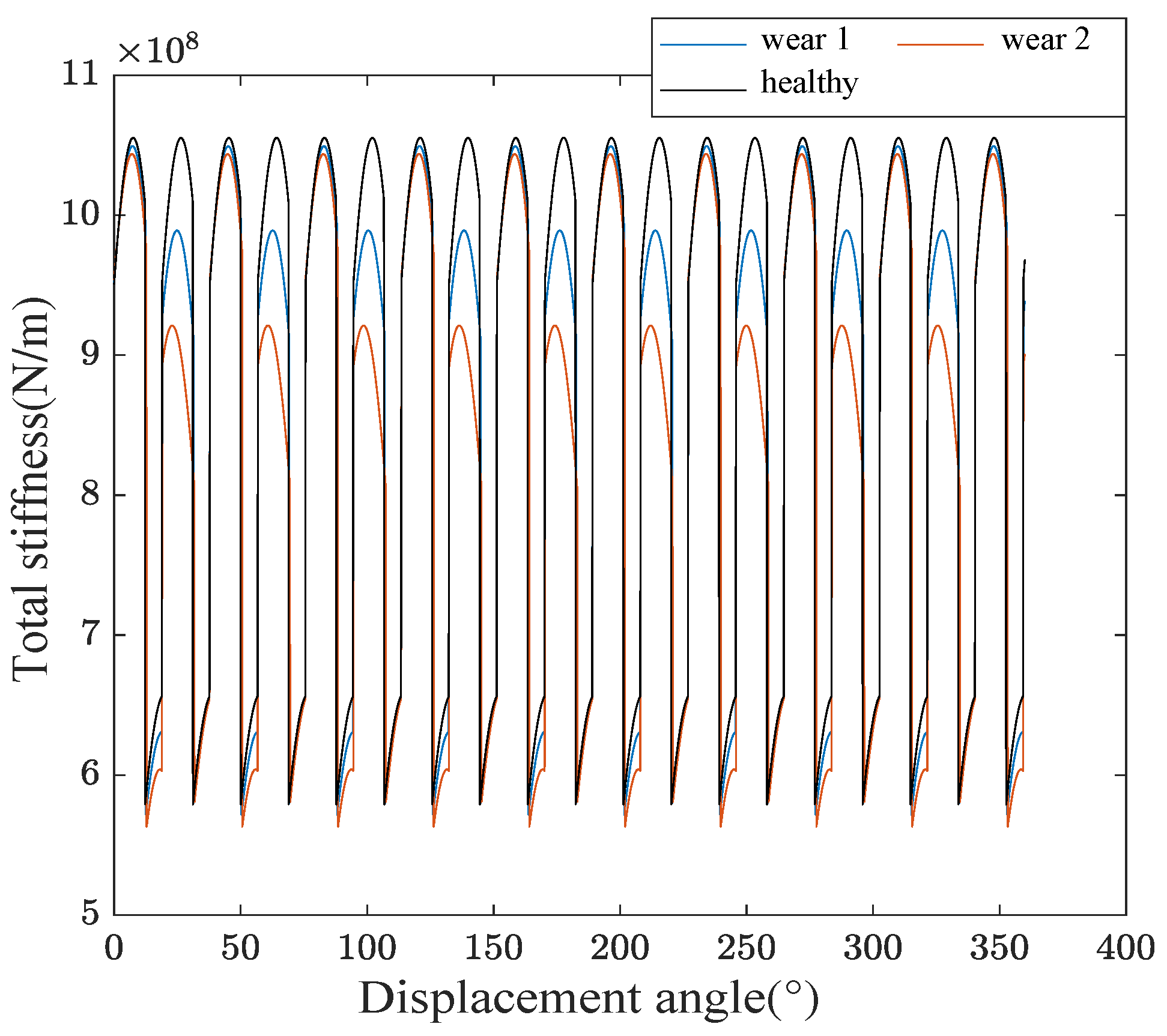
2.5. Wear Teeth Fault Modeling

As illustrated in Figure 6, wear is a common fault in gears, where material is removed from the tooth surface, resulting in profile changes at the contact point, notably a reduction in the tooth thickness represented by $d_h$. According to Wang et al. [23], the reduction is considered uniform on both sides of the tooth and constant along its height.

The new formulation for the tooth profile height $h_x$ is used in the following equations.

$$h_x=R_{b1}\left((\alpha +{\alpha }_2)cos\alpha -sin\alpha \right)-d_h$$

(26)

This fault also influences the angle of force application along the line of action, causing the angle ${\alpha }_1$ to change to angle $\gamma$. This angle is determined by the following expression.

$$\gamma =arctan(tan{\alpha }_1+d_h)$$

(27)

The expressions for bending, compressive, and shear rigidities are modified, while the Hertzian contact stiffness $k_h$ remains unchanged.

$$\frac{1}{k_b}={\int }_{-{\alpha }_1}^{{\alpha }_2}\frac{3D^2({\alpha }_2-\alpha )cos\alpha }{2EL{\left(({\alpha }_2-\alpha )cos\alpha -\frac{d_h}{R_{b1}}+sin\alpha \right)}^3}d\alpha$$

(28)

$$\frac{1}{k_a}={\int }_{-{\alpha }_1}^{{\alpha }_2}\frac{({\alpha }_2-\alpha )cos\alpha {sin}^2\gamma }{2EL\left(({\alpha }_2-\alpha )cos\alpha -\frac{d_h}{R_{b1}}+sin\alpha \right)}d\alpha$$

(29)

$$\frac{1}{k_s}={\int }_{-{\alpha }_1}^{{\alpha }_2}\frac{2.4(1+\nu )({\alpha }_2-\alpha )cos\alpha {cos}^2\gamma }{EL\left(({\alpha }_2-\alpha )cos\alpha -\frac{d_h}{R_{b1}}+sin\alpha \right)}d\alpha$$

(30)

with

$$\begin{array}{c}\hfill D=cos\gamma \left[({\alpha }_1+{\alpha }_2)sin{\alpha }_1+cos{\alpha }_1(\alpha -{\alpha }_2)sin\alpha -cos\alpha \right]+\\ \hfill sin\gamma \left[\frac{d_h}{R_{b1}}+sin{\alpha }_1-({\alpha }_1+{\alpha }_2)cos{\alpha }_1\right]\end{array}$$

(31)

The equations governing tooth wear are taken from [23] with adaptations to the type of teeth studied.

3. Gear Mesh Stiffness

3.1. Gear Mesh Stiffness at Healthy State

This period is defined as a full rotation (360°) divided by the number of teeth, whether for a single pair of teeth or for two pairs of teeth. With a pinion of 19 teeth, the contact period is $18.{95}^{\circ }$. This rigidity exhibits two different cases: one curve representing a maximum corresponding to double-pair contact and another curve representing a minimum corresponding to single pair contact. This rigidity is repeated until the gears complete a full rotation of 360°, and the corresponding graph is shown in Figure 7.

3.2. Gear Mesh Stiffness Under Broken Tooth Fault

According to the expression for total rigidity presented in Equation (7), if a tooth is missing, the remaining tooth will lose contact at the location of the missing tooth. This means that only one pair of teeth will be in contact during the contact period. Thus, where there was previously a double pair of teeth, there will now be a single pair, and where there was a single pair, the contact will be completely absent, as shown in Figure 8.

3.3. Gear Mesh Stiffness Under Crack Tooth Fault

Based on Equations (12)–(14) and with a crack size of q = 2.34 mm, Figure 9 illustrates the variation in the total engagement rigidity of the gears for each case. It is observed that this rigidity decreases for the tooth affected by the crack fault compared to the perfect state due to a less rigid contact.

3.4. Gear Mesh Stiffness Under Chipped Tooth Fault

In the scenario where part of the tooth is damaged, the simulation of several levels of fault severity for the pinion tooth, characterized by the dimensions z and b, is illustrated in Figure 4. The total rigidity of the gear can be calculated using Equation (17), as shown in Figure 10. The results presented demonstrate the different fault severities (z = 8 mm and $b1$ = 2, $b2$ = 2.25, $b3$ = 2.5, and $b4$ = 3 mm) and compare them to the healthy state. It is observed that the total engagement rigidity decreases with increasing fault severity for both scenarios.

3.5. Gear Mesh Stiffness Under Pitting Tooth Fault

Based on Equations (18)–(25), the mesh stiffness for pitting faults is illustrated in Figure 5. The analysis varied the number of pits ($n1$ = 3, $n2$ = 6, $n3$ = 9, and $n4$ = 12) while maintaining a constant radius of 1 mm. The locations and depths of the pits were fixed at 0.7 mm and 1 mm, respectively. The results, shown in Figure 11, clearly demonstrate that the total stiffness decreases as the fault severity increases. In the scenario where the radius is fixed, the stiffness varies within a consistent angular range.

3.6. Gear Mesh Stiffness Under Surface Wear Fault

We simulated a wear fault distributed across all the teeth of the pinion with varying severities, such as wear 1 of $d_h$ = 0.5 mm and wear 2 of $d_h$ = 1 mm, as shown in Figure 12. The effect of tooth wear on the engagement rigidity amplitude is clearly visible in the graph, where it decreases. Additionally, the amplitude of the engagement range for double-pair contact is slightly reduced compared to single-pair contact, where all the contact is made by a single tooth.

3.7. Modeling the Vibrational Dynamics of a Gearbox

After calculating the rigidity, turn to examining the vibratory response of a gearbox, adopting the mathematical model of torsional and lateral vibration in [24]. This model represents a single-stage gearbox system, as illustrated in Figure 13. It is defined by two main parameters, stiffness and damping, and encompasses both linear and rotational equations of motion for the system. The model describes a system with six degrees of freedom, subjected to an electric driving torque $M_1$ and influenced by an external torque $M_2$. It is specifically designed to analyze the effects of evolving gear faults on the system’s vibratory response. In this study, we assume that all gears are perfectly assembled rigid bodies, with ideal geometries. Friction between the teeth is neglected for simplicity [24]. The following notations will be used throughout this study:

• $I_m$—mass moment of inertia of the motor;
• $l_b$—mass moment of inertia of the load;
• $I_1$—mass moment of inertia of the pinion;
• $I_2$—mass moment of inertia of the gear;
• $M_1$—input motor torque;
• $M_2$—output torque from load;
• $m_1$—mass of the pinion;
• $m_2$—mass of the gear;
• $R_{b1}$—base circle radius of pinion;
• $R_{b2}$—base circle radius of gear;
• $k_p$—torsional stiffness of the input flexible coupling
• $k_g$—torsional stiffness of the output flexible coupling
• $c_p$—damping coefficient of the input flexible coupling;
• $c_g$—damping coefficient of the output flexible coupling;
• $k_{x1}$—horizontal radial stiffness of the input bearings;
• $k_{x2}$—horizontal radial stiffness of the output bearings;
• $k_{y1}$—vertical radial stiffness of the input bearings;
• $k_{y2}$—vertical radial stiffness of the output bearings;
• $c_{x1}$—horizontal radial viscous damping coefficient of the input bearings;
• $c_{x2}$—horizontal radial damping coefficient of the output bearings;
• $c_{y1}$—vertical radial damping coefficient of the input bearings;
• $c_{y2}$—vertical radial damping coefficient of the output bearings;
• $k_t$—mesh stiffness;
• $c_t$—mesh damping coefficient;
• $x_1$—linear displacement of pinion in the direction parallel to teeth in mesh (the x direction);
• $x_2$—linear displacement of gear in the x direction;
• $y_1$—linear displacement of pinion in the direction vertical to teeth in mesh (the y direction);
• $y_2$—linear displacement of gear in the y direction;
• ${\theta }_m$—angular displacement of motor;
• ${\theta }_1$—angular displacement of pinion;
• ${\theta }_2$—angular displacement of gear;
• ${\theta }_b$—angular displacement of load.

Given that friction is not considered, the vibration in the x direction naturally decays due to damping. In this study, we focus solely on the motion in the y direction.

As mentioned in [24], the vertical motion equations (in the y direction) for the pinion and gear are

$$m_1{\ddot{y}}_1+F_u+F_{uc}=-F_k-F_c$$

(32)

$$m_2{\ddot{y}}_2+F_l+F_{lc}=F_k+F_c$$

(33)

$$I_1{\ddot{\theta }}_1=M_{pk}+M_{pc}-R_{b1}(F_k+F_c)$$

(34)

$$I_2{\ddot{\theta }}_2=-M_{gk}-M_{gc}+R_{b2}(F_k+F_c)$$

(35)

$$I_m{\ddot{\theta }}_m=M_1-M_{pk}-M_{pc}$$

(36)

$$I_b{\ddot{\theta }}_b=-M_2+M_{gk}+M_{gc}$$

(37)

Such that

$$F_k=k_t(R_{b1}{\theta }_1-R_{b2}{\theta }_2-y_1+y_2)$$

(38)

$$F_c=c_t(R_{b1}{\dot{\theta }}_1-R_{b2}{\dot{\theta }}_2-{\dot{y}}_1+{\dot{y}}_2)$$

(39)

$$F_u=k_1{y}_1$$

(40)

$$F_{uc}=c_1{\dot{y}}_1$$

(41)

$$F_l=k_2{y}_2$$

(42)

$$F_{lc}=c_2{\dot{y}}_2$$

(43)

$$M_{pk}=k_p({\theta }_m-{\theta }_1)$$

(44)

$$M_{pc}=c_p({\dot{\theta }}_m-{\dot{\theta }}_1)$$

(45)

$$M_{gk}=k_g({\theta }_2-{\theta }_b)$$

(46)

$$M_{gc}=c_g({\dot{\theta }}_2-{\dot{\theta }}_b)$$

(47)

With the established model, the next step is to use these sets of equations for a dynamic simulation when the gear is either healthy or faulty. We assumed that the vertical radial stiffness of the input bearings, $k_1$, and that of the output bearings, $k_2$, are identical and constant. The damping coefficient of the input bearings $c_1$ and that of the output bearings $c_2$ are identical and equal to a constant $c_r$. The torsional stiffness of the input flexible coupling $k_p$ and that of the output elastic coupling $k_g$ are both equal to a constant $k_c$. The elastic coupling damping of the input $c_p$ and that of the output elastic coupling $c_g$ are equal to $c_c$. Additionally, the engagement damping coefficient $c_t$ is set to be proportional to the total engagement stiffness $k_t$ [20].

To solve this problem, the stiff ordinary differential equation (ode15) function is used, which is capable of handling such discontinuities. Then, their vibratory behavior is simulated for each case of severity, as indicated in

Table 1. Emulated gear states.

Gear State	Severity
Healthy	/
Broken	/
Crack	q = 2.34 mm
Chipped	b = 2.5 mm, z = 8 mm
Pitting	n = 1, r = 1 mm
Wear	$dh$ = 0.2 mm

, for a duration of 0.1 s, and the results are presented in Figure 14.

Figure 14 illustrates the vertical vibratory response of the pinion in various case studies, including the healthy state and different types of faults, pitting, chipped, cracks, wear, and broken, for specific severity levels as indicated in Table 1.

4. Proposed Diagnosis Methodology

4.1. Feature Extraction and Selection

After the signal preparation, the feature extraction for each signal is initiated. For this, statistical indicators in the time domain are calculated for each segment of the signal for each class. These indicators include: mean ($\mu$), standard deviation ($\sigma$), skewness ($SK$), root mean square ($RMS$), kurtosis ($KT$), crest factor ($CF$), entropy value ($EP$), shape factor ($SF$), operator energy ($EOP$), fluctuation factor ($FJ$), impulsiveness factor ($IF$), and the two factors $S_r$ and $S_{\alpha }$.

To enhance class separability, the determination of discriminant features is performed to maximize inter-class variance (dispersion between classes) relative to intra-class variance (dispersion within a class) [8]. For M classes and a given feature $\alpha$, the Fisher criterion $J\left(\alpha \right)$ is expressed as

$$J\left(\alpha \right)=\sum _{i=1}^M\sum _{j=1}^{M-1}\frac{{(m_i\left(\alpha \right)-m_j\left(\alpha \right))}^2}{N_i{\sigma }_i^2\left(\alpha \right)+N_j{\sigma }_j^2\left(\alpha \right)}$$

(48)

where

• $m_i$: Mean value of feature $\alpha$ for class i.
• ${\sigma }^2$: Variance of feature $\alpha$ for class i.
• N: Number of samples in class i.

In the numerator: ${(m_i\left(\alpha \right)-m_j\left(\alpha \right))}^2$ represents the squared distance between the means of classes i and j. A larger distance indicates that the classes are better separated.

In the denominator: $N_i{\sigma }_i^2\left(\alpha \right)+N_j{\sigma }_j^2\left(\alpha \right)$ reflects the dispersion or variability within the two classes. If the variances are large, it makes separation more difficult.

Although this criterion allows for ranking the extracted features according to their discriminative power, the optimal number of features to retain must be determined empirically through validation with a decision rule. The normalized contribution of each feature $\alpha$ can be calculated using Equation (49).

$$J_{N_j}(\%)=\frac{100\times J\left({\alpha }_j\right)}{{\displaystyle \sum _{i=1}^d}J\left({\alpha }_i\right)}$$

(49)

4.2. Fault Detection

According to the Fisher criterion, the three most relevant indicators for detection are RMS, CF, and $S_r$. Although the criterion allows for ranking the calculated indicators in descending order of importance, these three indicators are used to form the dataset. For each class, 80% is randomly selected for training and 20% for test.

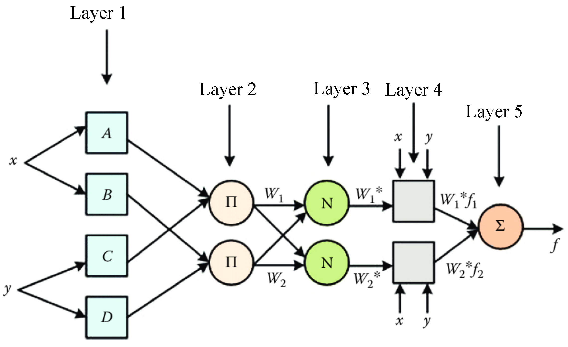
ANFIS (Adaptive Neuro-Fuzzy Inference System) is a sophisticated hybrid intelligent framework that synergistically combines neural network learning capabilities with fuzzy logic reasoning, as illustrated in Figure 15. The architecture comprises five functionally distinct layers that work in tandem to process information: the initial Fuzzification Layer transforms crisp inputs into linguistic variables through membership functions; the subsequent Inference Layer applies fuzzy IF–THEN rules to generate appropriate weighting factors; the Normalization Layer scales these weights proportionally; then, the Aggregation Layer combines the normalized outputs; and finally, the Defuzzification Layer converts the fuzzy conclusions into actionable numerical outputs. This multilayered structure employs adaptive network parameters including connection weights ($W_1$, $W_2$), normalization operators (N), and a series of intermediate computational nodes ($W_1^{\ast }$, $W_2^{\ast }$, $W_1^{\ast }{f}_1$ through $W_2^{\ast }{f}_2$) that collectively enable the system to learn complex input–output relationships while maintaining interpretability through fuzzy rules [25]. The unique integration of gradient-based learning from neural networks with the approximate reasoning of fuzzy systems allows ANFIS to effectively model highly nonlinear, uncertain processes across various domains, from industrial control to predictive analytics, while offering advantages in both accuracy and transparency compared to conventional approaches. The system’s adaptive nature permits continuous refinement of membership functions and rule bases through exposure to training data, making it particularly suitable for applications requiring both learning capacity and human-understandable decision logic [16].

The dataset is prepared as follows: The first three columns represent the inputs (selected indicators), and the last column represents the desired output for our ANFIS model. After generating the dataset, create the initial FIS system with two membership functions and begin the learning phase by selecting the appropriate training options, as follows:

• Learning method: Hybrid method using least squares and gradient back-propagation.
• Error tolerance: 0 (used as a learning stopping criterion, related to the size of the error).
• Number of iterations: Set to 200 to achieve error stabilization.

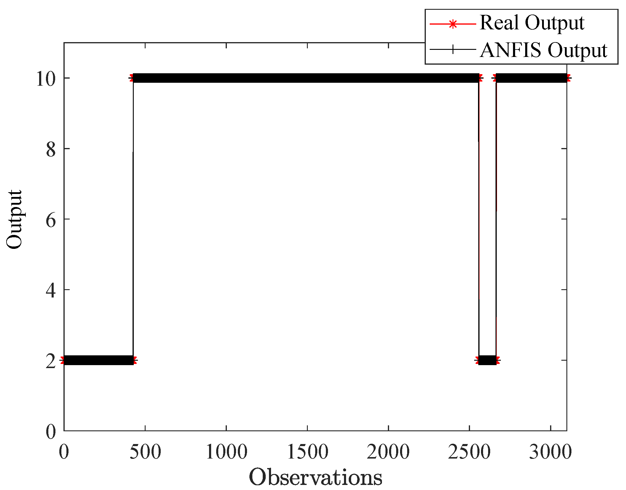
After training and testing, the detection result is 100%, as illustrated in Figure 16.

Figure 16 shows the prediction versus the observations. The observations include all the training data (2556 samples: 426 samples for the healthy state and the rest for the five fault classes) and the testing data (642 samples: 107 samples for the healthy state and the rest for the five fault classes). The outputs are limited to two classes only (2 for the healthy state and 10 for the faulty state, where different faults are mixed). The figure demonstrates a perfect classification of the entire dataset, reflecting the effectiveness of Fisher’s criterion for selecting the most discriminative features, as well as the suitability of the ANFIS machine learning network for this detection task.

4.3. Fault Diagnostic

Based on the Fisher criterion, which evaluates the relevance of indicators in the fault diagnosis phase of the gearbox, certain indicators stand out for their ability to effectively discriminate between different faults. These key indicators provide essential information for accurately identifying and classifying gearbox faults. The three indicators selected for diagnosis are the impulse factor ($IF$), the mean value ($\mu$), and the operator energy ($EOP$). Using the three indicators to train the ANFIS model results in a dataset with 533 samples for each fault. Divide each class into 80% for training and 20% for test. The other parameters of the ANFIS model are the same as those used for detection. The diagnostic result is 100%, as illustrated in the confusion matrix in Figure 17.

The diagonal elements of the confusion matrix represent correct classifications, while the off-diagonal elements reflect misclassifications between classes. As shown in the confusion matrix in Figure 17, all off-diagonal elements are zero, and the diagonal elements contain the exact number of correctly classified samples, which is 107 for each class. This reflects the high quality of the classification achieved, with an accuracy of 100%. Such a result highlights the effectiveness of combining the Fisher criterion for feature selection with ANFIS for classification.

4.4. Experimental Validation of the Proposed Approach

In this step, the diagnostic approach presented in the previous two sections was validated experimentally. This was accomplished using a dataset created by Fedala et al. [27].

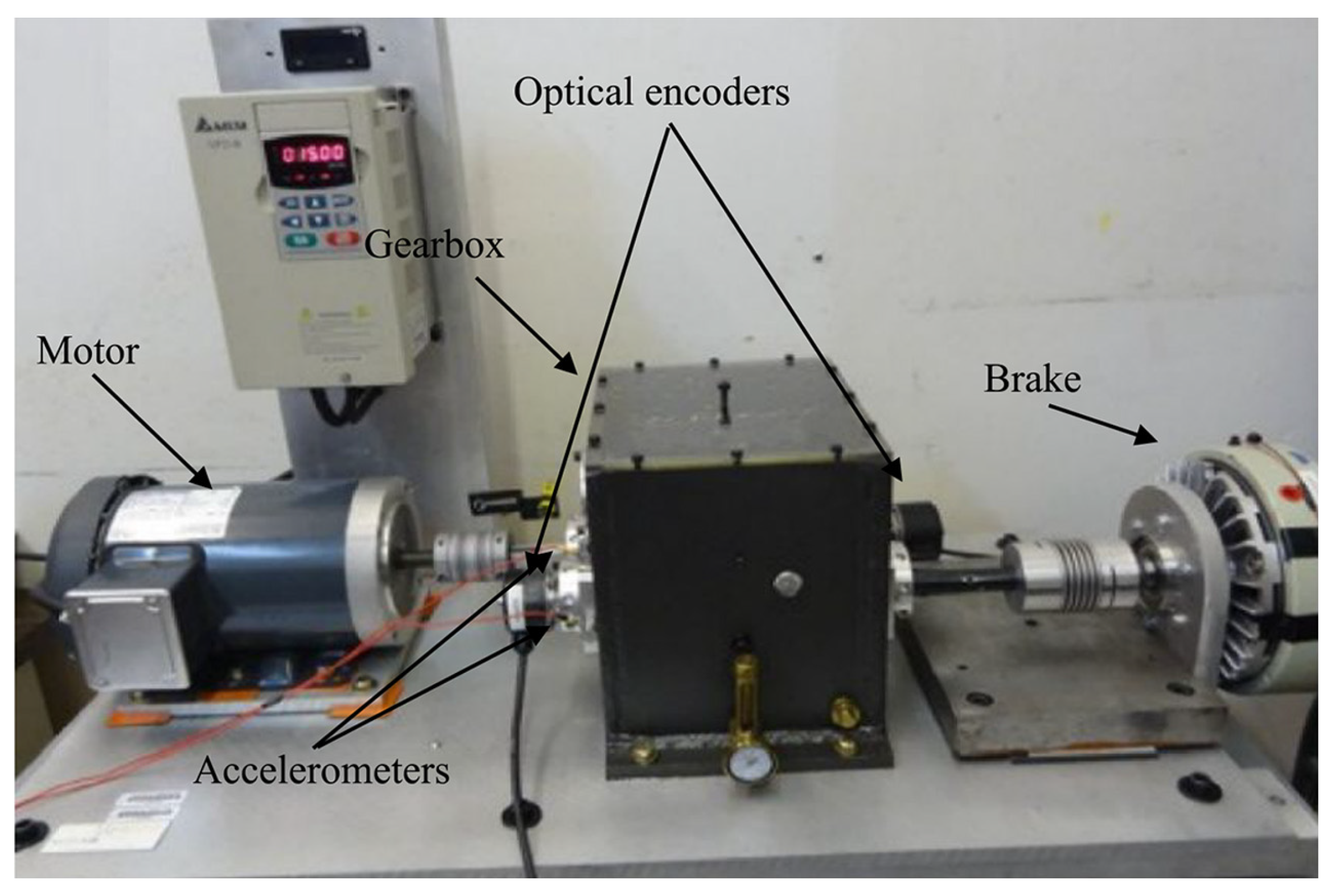
The gearbox test bench, illustrated in Figure 18, consists of a direct current (DC) motor controlled by a speed regulator. This motor, which can reach a speed of 3600 RPM, is connected to the gearbox via a flexible coupling, with an encoder installed at both the input and output shafts. At the output, the gearbox is linked to a brake through another flexible coupling, allowing for load control. The gearbox comprises a single-stage spur gear system with a 25/56 tooth ratio.

To assess the effectiveness of the proposed method, six gears with different faults were considered during the experiment. The first gear is in Good state (G), while the others have various faults: a Root Crack (RC), a Chipped Tooth in Length (CTL), a Chipped Tooth in Width (CTW), a Missing Tooth (MT), and General Surface Wear (GSW), as shown in Figure 19.

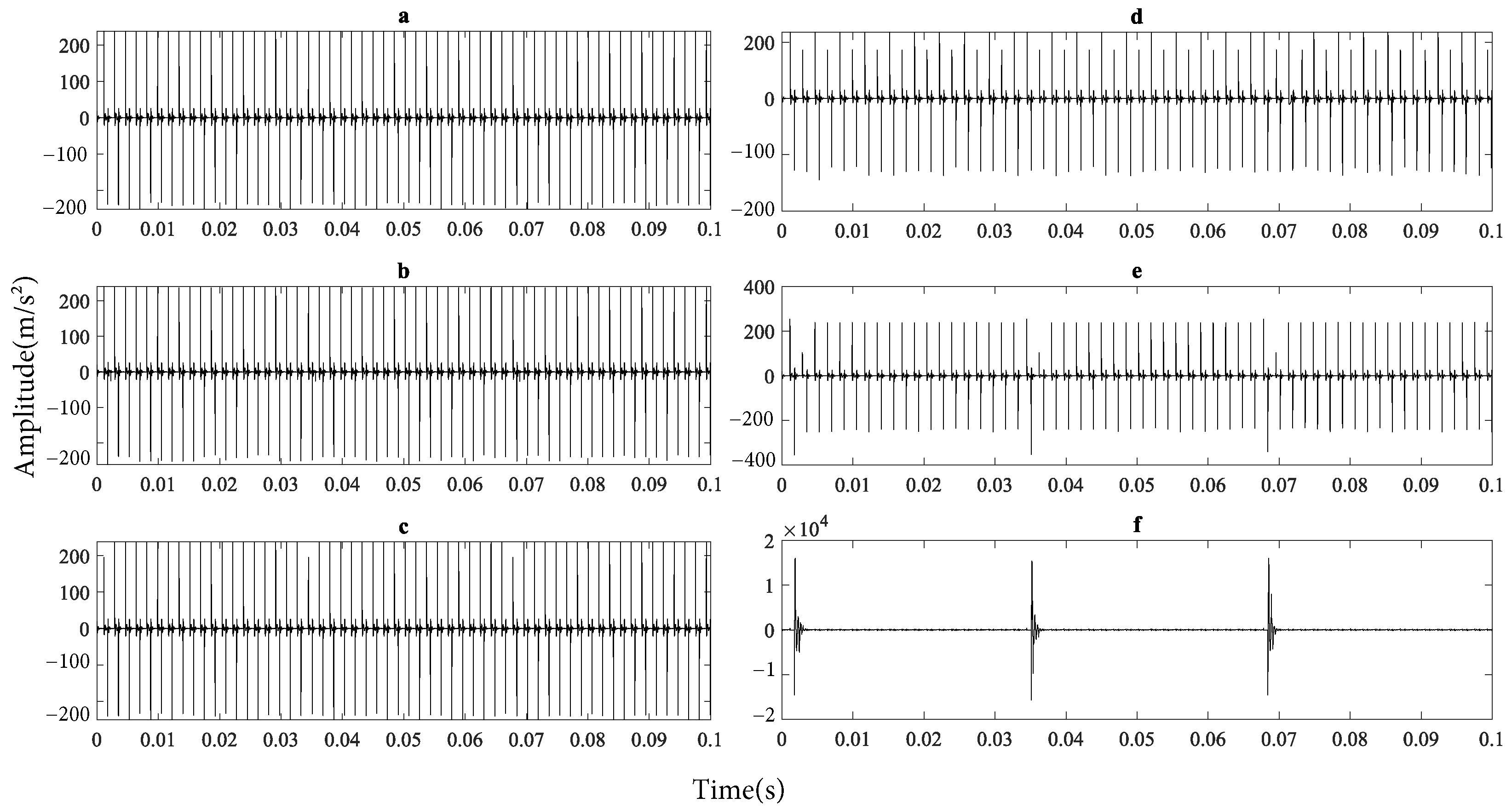
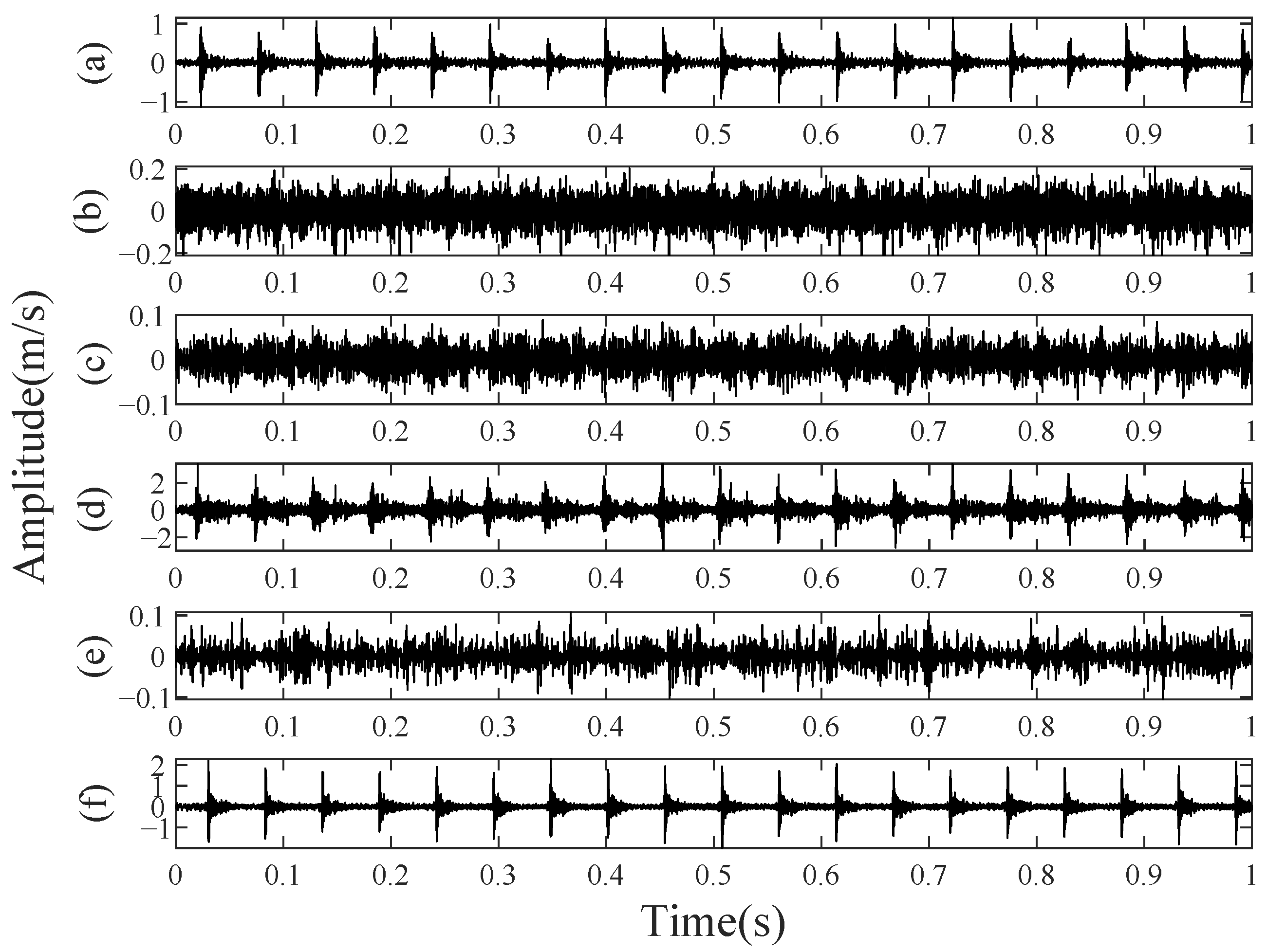
The accelerometer sampling frequency was set to 125 kHz with a 27 kHz filter cutoff frequency, using a 30 s acquisition duration. The diagnostic validation approach was implemented at an operating speed of 1200 RPM and a torque of 11 Nm, yielding the vibrational signals shown in Figure 20.

When comparing the experimental signals in Figure 20 with those obtained from the model in Figure 14, the two classes exhibiting impulsive characteristics are missing tooth and chipped tooth. These two faults increase dynamic transmission error, resulting in more significant tooth impact [28]. The other faults have a less significant impact, making their signatures comparable to noise levels.

Each measurement was subdivided into 120 segments of 0.25 s. The dataset is divided into 80% for training and 20% for testing to perform training with the ANFIS model. The selection of the most relevant indicators according to the Fisher criterion identified the following three indicators: standard deviation ($\sigma$), kurtosis ($KT$), and root mean square ($RMS$).

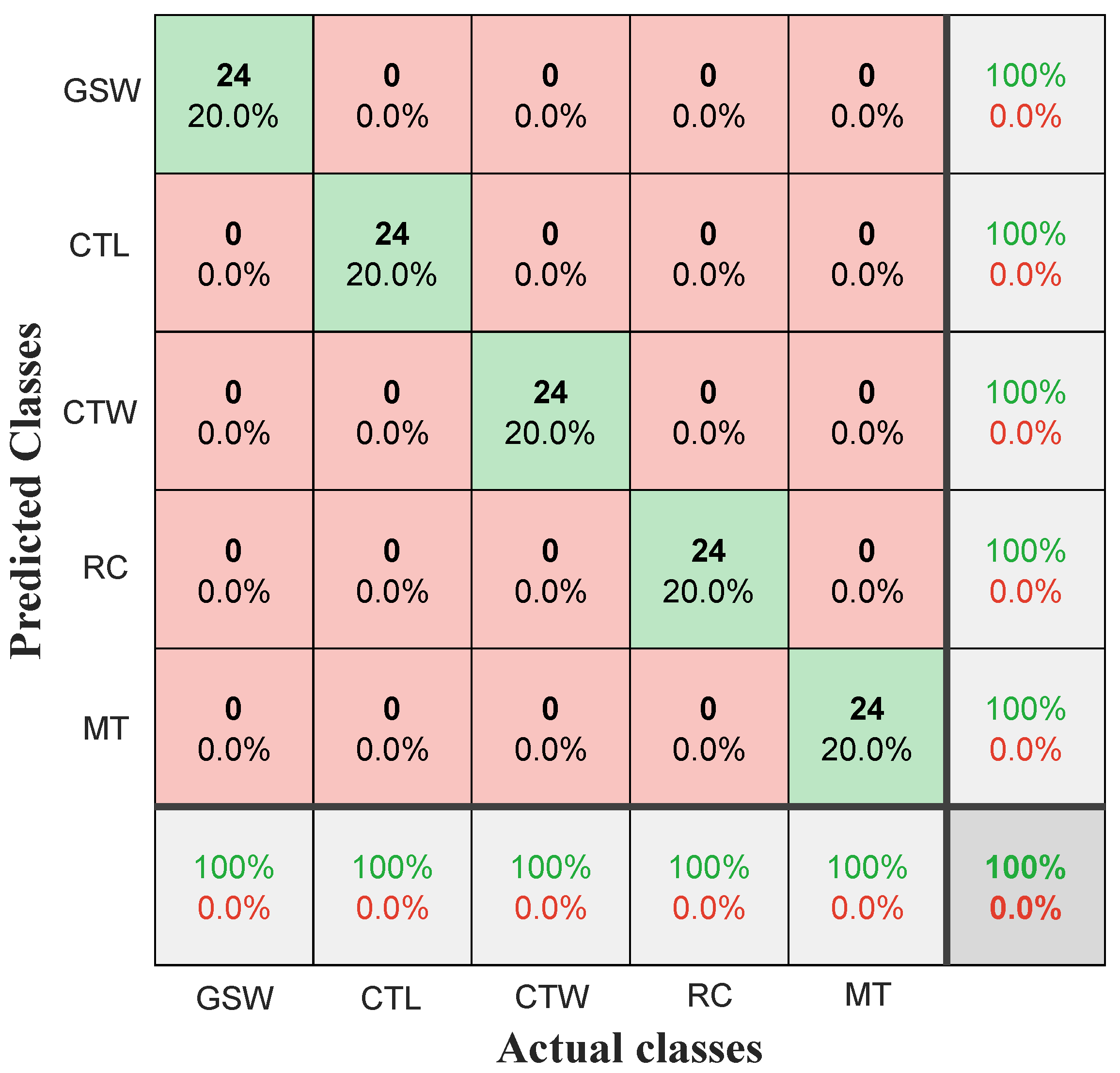
The classification accuracy rate is 100%. The confusion matrix in Figure 21 presents the test results for each class.

The confusion matrix shown in Figure 21 was obtained by applying the proposed methodology to the experimental data. As illustrated, the off-diagonal (red cells) elements are all zero, while the diagonal elements (green cells) display a perfect classification rate of 24/24 samples for each class (displayed in bold). These results demonstrate the effectiveness of the approach, which combines Fisher’s criterion for feature selection and ANFIS for classification. The methodology not only accurately distinguishes between different fault categories but also assesses their severity, thereby facilitating the diagnosis of emerging faults.

The ANFIS learning results were compared with well-known machine learning approaches, including Support Vector Machines (SVM), k-Nearest Neighbors (k-NN), and Random Forest (RF). These methods are widely used, particularly in fault diagnosis applications [29]. The classification accuracy reached 96.67% for SVM and 100% for both k-NN and Random Forest. Compared to the identical 100% accuracy achieved by ANFIS, these results highlight the effectiveness of the Fisher criterion feature selection technique, which enables robust learning across different network architectures.

Another comparison with a recent framework was conducted using the same dataset [30], where vibration signals were processed through the following methodology: First, the signal is decomposed using Maximal Overlap Discrete Wavelet Packet Transform. Next, the autocorrelation of the squared envelope is computed, followed by kurtosis calculation for each autocorrelation. The features extracted through this process are then used to train a Radial Basis Function Neural Network, achieving 100% fault detection and diagnosis accuracy—identical to the results obtained in our paper using time-domain signal analysis with ANFIS learning.

5. Conclusions

This paper investigates the potential of artificial intelligence techniques for fault detection and diagnosis in gearboxes, with a focus on modeling vibrational responses and leveraging machine learning. The main objective was to demonstrate how these innovative methods can enhance the predictive maintenance of gearboxes, thereby increasing their reliability and extending their operational lifespan. By modeling gear tooth rigidity, this study analyzed the impact of gear faults on the vibration response of the system. The findings revealed that a reduction in rigidity due to faults can significantly affect the performance of rotating systems, underscoring the importance of accurate fault diagnosis. To develop reliable fault detection and classification models, machine learning algorithms were applied to the vibration data collected during experiments. Feature selection based on the Fisher criterion was employed to identify the most discriminate features, enhancing the models’ ability to distinguish between healthy and faulty states effectively. This step was crucial in improving the performance and accuracy of the fault diagnosis models. Among the machine learning techniques used, fuzzy logic methods and ANFIS (Adaptive Neuro-Fuzzy Inference System) proved particularly effective in the learning process. These techniques delivered strong results in fault classification, showing high accuracy when tested on independent data. Trained on a comprehensive dataset of vibration signatures, the models outperformed traditional expert-based rule methods in both fault detection and classification tasks. In summary, the integration of feature selection based on the Fisher criterion, along with advanced machine learning techniques, demonstrated a significant advancement in gearbox fault diagnosis. This approach not only strengthens predictive maintenance strategies but also improves the overall performance and reliability of gearboxes. The use of modeling allows for the anticipation and reduction of relevant features prior to training with a suitable network, enabling the precise specification of the hardware required for deploying the proposed solution. Finally, a comparative analysis with other machine learning methods and a benchmark against a state-of-the-art framework confirmed the effectiveness of the ANFIS model for fault diagnosis.

One of the most interesting directions would be to extend our approach to prognostics, which involves monitoring the progression of fault severity and estimating the remaining useful life of each faulty component. This extension would not only detect existing faults but also predict their progression and plan maintenance interventions in a more proactive and optimized manner.