Abstract
Magnetic flux leakage (MFL) detection is widely used in the non-destructive testing of pipelines. Inversion is a key step in MFL detection, and iterative inversion based on an optimization algorithm is an effective method for constructing the 3-D profile of defects in pipelines. However, conventional inversion algorithms suffer from weak convergence ability and are prone to local optima, which can lead to significant errors in the results. To improve the algorithm’s convergence and result accuracy, this paper proposes a “continuity correction” strategy based on geometric features of defects, which examines the relative depth value of each depth point and corrects the values of implausible points. On this basis, this paper combines the secretary bird optimization algorithm (SBOA) with the differential evolution strategy and the perturbation strategy to enhance the search capability. Through an accuracy experiment and a robustness experiment on an experimental platform, it is demonstrated that the method outperforms conventional algorithms in terms of accuracy and robustness against interference when constructing the 3-D profile of defects.
1. Introduction
Pipelines are important carriers of energy transportation, and the non-destructive testing (NDT) of pipelines provides an important guarantee for secure and stable operation [1]. NDT is an effective method of assessing condition and damage without destroying samples. Common NDT methods include magnetic flux leakage (MFL) testing, eddy current testing, ultrasonic testing, and so on [2]. MFL testing is widely used due to its simplicity, real-time detection capability, and high degree of automation [3]. Thus, MFL-based defect profile construction plays an important role in detecting pipeline condition and damage.
Defect inversion is the process of solving for the geometric profiles of defects reversely based on the measured MFL signals. The methods are mainly divided into direct inversion methods based on machine learning and iterative inversion methods based on optimization algorithms. Direct inversion methods use machine learning methods to directly establish mathematical relationships between MFL signals and defect geometric features without considering the physical process of signal generation. In this field, Yu et al. [4] proposed WT-STACK, which improves accuracy and robustness but relies on expert experience. Wu et al. [5] proposed a reinforcement learning-based algorithm, which reduces computational cost but depends on training data quality. Liu et al. [6] proposed a cascaded attention feature hybrid network, which enhances accuracy and robustness but depends on feature selection and model complexity. Yuksel et al. [7] proposed a novel cascaded deep learning model, which enhances robustness and efficiency but relies on effective feature representation. Khodayari-Rostamabad et al. [8] used support vector regression and kernel-based learning methods to address defect detection and depth estimation in MFL image analysis. Pasadas et al. [9] used a multi-level support vector machine (SVM) model combined with eddy current testing (ECT) to classify surface and sub-surface cracks of varying lengths and depths in aluminum plates. Direct inversion based on machine learning is simpler and faster but requires a large amount of data to train its mathematical model. And, there is a risk of poorer results in the inversion that differs from the training conditions.
Iterative inversion based on MFL signals uses an optimization algorithm to solve the defect profile inversely, which is characterized by higher precision and wider applicability. It includes the forward modeling process and the inversion process. Forward modeling simulates the MFL field distribution of defects based on their geometrical features. In this field, Feng et al. [10] gave an analytical expression for the leakage magnetic field based on the 3-D magnetic dipole model. Zhang et al. [11] proposed the Magnetic Charge Element Method, which reduces computation time but depends on proper discretization and external field estimation. Gao et al. [12] and Liu et al. [13] both presented 3-D MFL signals based on non-uniform magnetic charge models, improving defect characterization accuracy but increasing computational complexity. This paper uses uniform magnetic charge model for forward modeling.
An inversion algorithm is the key to iterative inversion. For 2-D inversion, there have been a number of studies. Amineh et al. [14] used a space mapping-based optimization strategy combining FEM and analytical models to solve the inversion problem. Priewald et al. [15] used a nonlinear finite element method (FEM) combined with Gauss–Newton optimization to reconstruct surface defect profiles. Han et al. [16] combined cuckoo search and particle filters in a strategy which demonstrates good robustness for 2-D inversion problems but requires a longer computation time. Lu et al. used the finite-element method (FEM) and a weighting conjugate gradient algorithm under different velocity conditions [17] and improved particle swarm optimization with self-adaptive inertia weight and the speed-updating strategy to achieve fast convergence [18]. The former focuses on accuracy and robustness under high-speed detection, while the latter emphasizes fast convergence and computational efficiency. Li et al. [19] proposed a modified harmony search algorithm, which can balance the accuracy and efficiency of 2-D inversion, but performed sensitive to parameter settings. The 3-D iterative inversion constructs the profiles of the defects more in detail and accurately, which is catering more to engineering requirements. Hou et al. [20] proposed a target focusing-modified beetle swarm optimization (TF-MBSO) algorithm, which achieved relatively accurate 3-D inversion with a degree of freedom of 4 4 but performs poorly for inversions of a higher degree of freedom and lacks robustness verification. Despite the limited studies on 3-D iterative inversion, considerable progress has been made in related optimization algorithms. Zhao et al. [21] proposed an improved Harris hawk optimization (HHO) algorithm for reactive power optimization. Li et al. [22] used an improved Whale optimization algorithm (WOA) for electromagnetic inversion problems. In addition, the PID-based search algorithm [23] (PSA), secretary bird optimization algorithm [24] (SBOA), and black-winged kite algorithm [25] (BKA) exhibited strong global search capabilities, which are suitable for MFL-based defect inversion at a low degree of freedom. But, when directly applied to 3-D inversion with higher degrees of freedom, these algorithms still yield low-quality local optimal solutions.
In general, a higher degree of freedom allows for a more precise representation of the defect profile, yet the error tends to increase due to the algorithm’s random search, which is the current challenge for 3-D inversion. Additionally, conventional inversion methods only focus on the deviation between the signals, which cannot completely reflect the deviation between inverted and actual profiles in the iterative process, ignoring the geometric characteristics of the inverted profiles and the plausibility of the results. This leads to local optima, weak convergence capability, low accuracy, and poor robustness. To address such issues, a “continuity correction” strategy is proposed based on the gradual variation of depth in actual defects. By examining whether the depth values at each point excessively deviate from the surrounding region, the strategy adjusts implausible depth values, thus helping the inversion process shift away from local optima. On this basis, this paper combined the secretary bird optimization algorithm with the differential evolution strategy and the perturbation strategy. The main contributions of this paper are as follows:
- The continuity correction strategy is proposed to adjust the implausible depth values and help the inversion process shift away from local optima. This strategy enhances the accuracy of 3-D inversion, particularly in estimating the values at deeper points.
- The differential evolution strategy and perturbation strategy enhanced the search capability and fitting ability of SBOA, improving the accuracy of inverted profiles.
2. Forward Modeling
2.1. Measurement of MFL Signals in Pipelines
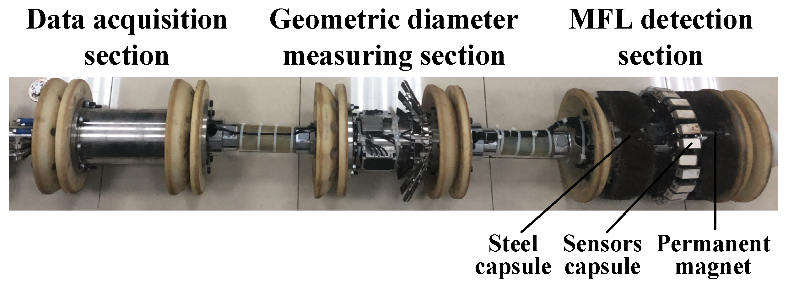
The pipeline detector used in this paper is shown in Figure 1, which was independently designed for MFL inspection applications. It consists of the MFL detection section, the diameter measuring section, and the data acquisition section. The MFL detection section is mounted with 40 mm steel brushes externally to separate the detector from the pipeline. N52-grade permanent magnets are used to magnetize the pipe wall to saturation. A total of 24 sensor capsules are evenly distributed around the circumference of the magnetic leakage node.
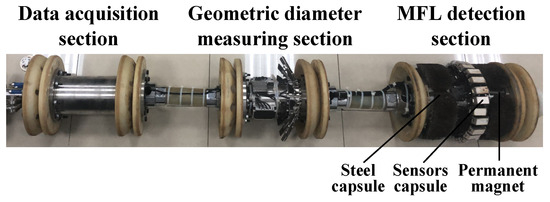
Figure 1.
Pipeline detector.
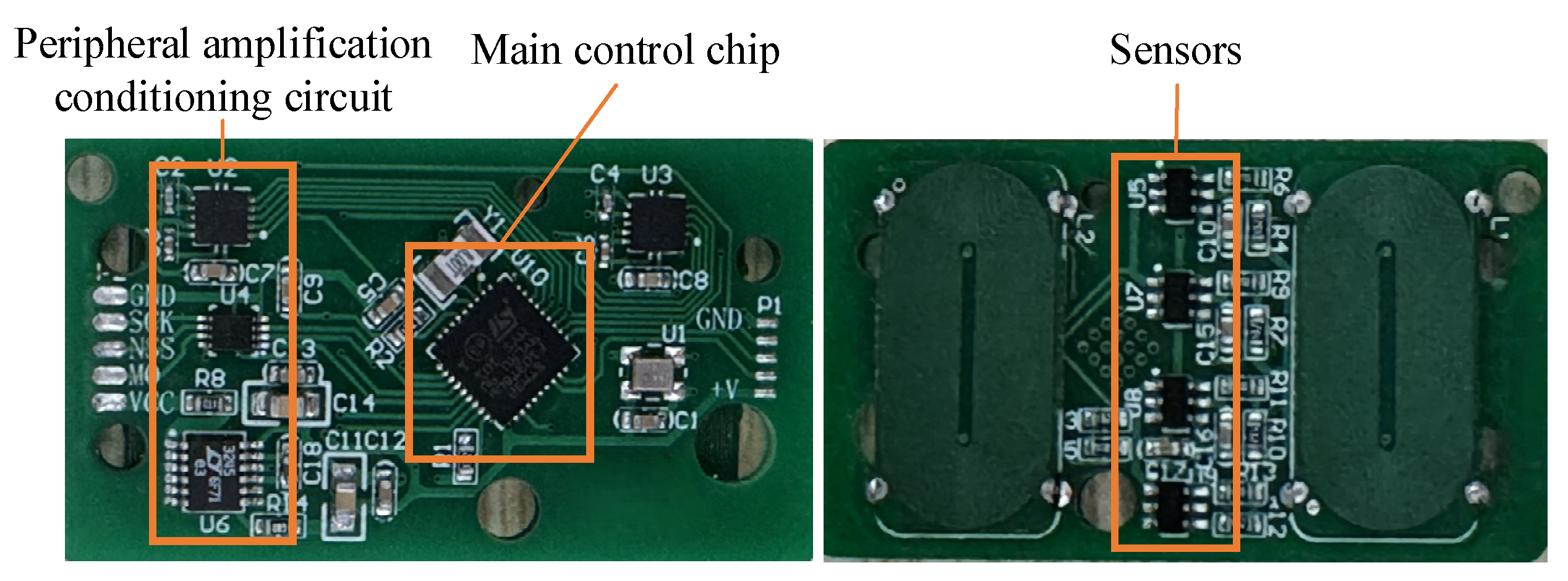
The core of each sensor capsule is the control circuit and four three-axis Hall sensors, as shown in Figure 2. The sensor model is TLE493DW2B6 (Infineon Technologies AG, Neubiberg, Germany). Each sensor has a detection sensitivity of 3.125 mV/G, a sampling range of ±670 Gs, a minimum measurement accuracy of 0.1 Gs, and a supply voltage of 4.5~10 V. It sets sampling points every 2 mm in the axial direction of the pipeline and every 6.5 mm in the circumferential direction.

Figure 2.
The circuit with sensors.
The MFL signals at sample points can be measured with the detector. Measured MFL signals can form an observation matrix based on the positions of the sampling points.
2.2. MFL Signal of the Defect
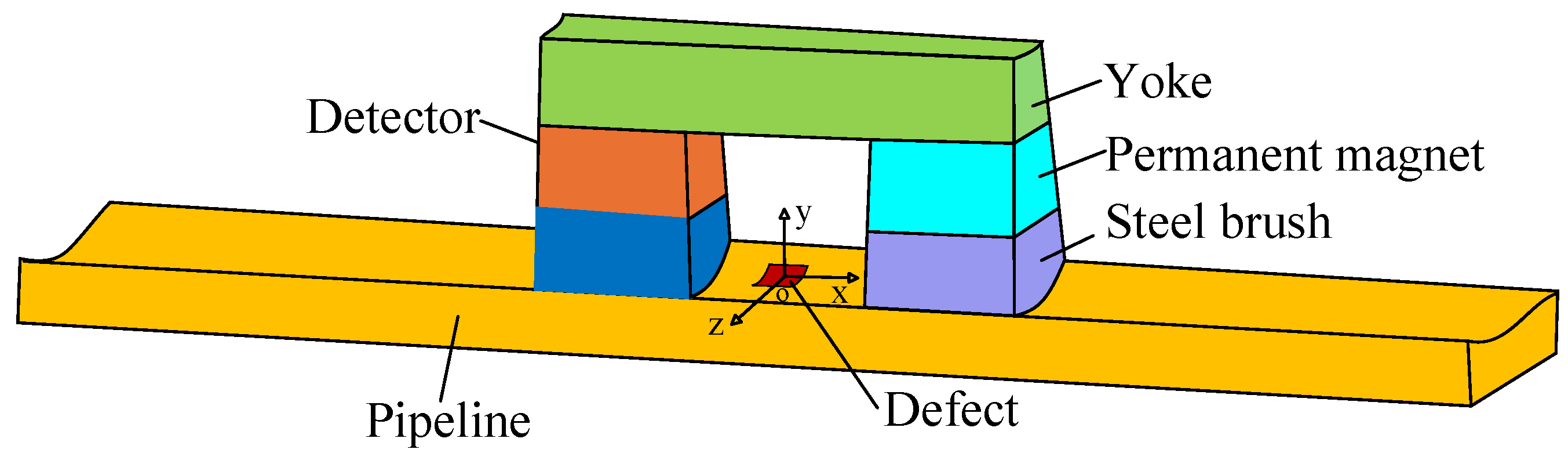
To better describe the 3-D MFL signals, a coordinate system is established based on the axial, radial, and circumferential directions of the pipeline. The X-axis, Y-axis, and Z-axis correspond to the axial, radial, and circumferential directions of the pipeline, respectively. The detection principle model is shown in Figure 3. This paper utilizes axial MFL signals to construct the 3-D profile.
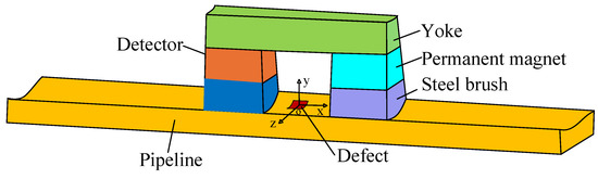
Figure 3.
The detection principle model.
Each defect can be divided into several segments of equal length and width. A higher degree of freedom in defect segmentation enables a more precise reconstruction of the profile. The MFL signals from each segment can be modeled as the magnetic field of a magnetic dipole layer. The 3-D magnetic field distribution of a magnetic dipole layer has been elaborated in detail [16] and will not be reiterated in this paper.
2.3. Forward Modeling and Profile Reconstruction
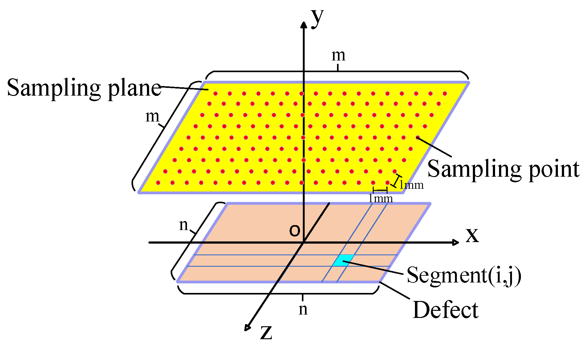
In Figure 4, the defect is divided into n n identical segments, with each segment represented by a depth point. The value at depth point (i,j) is . The n n depth values form a depth matrix , which characterizes the 3-D profile of the defect.

Figure 4.
Sampling points.
The sampling intervals of the interpolated points are 1 mm along both the x-axis and z-axis. To estimate the axial MFL signals at m m sampling points in the sampling plane, the axial signal distribution corresponding to each depth point (i,j) needs to be superimposed:
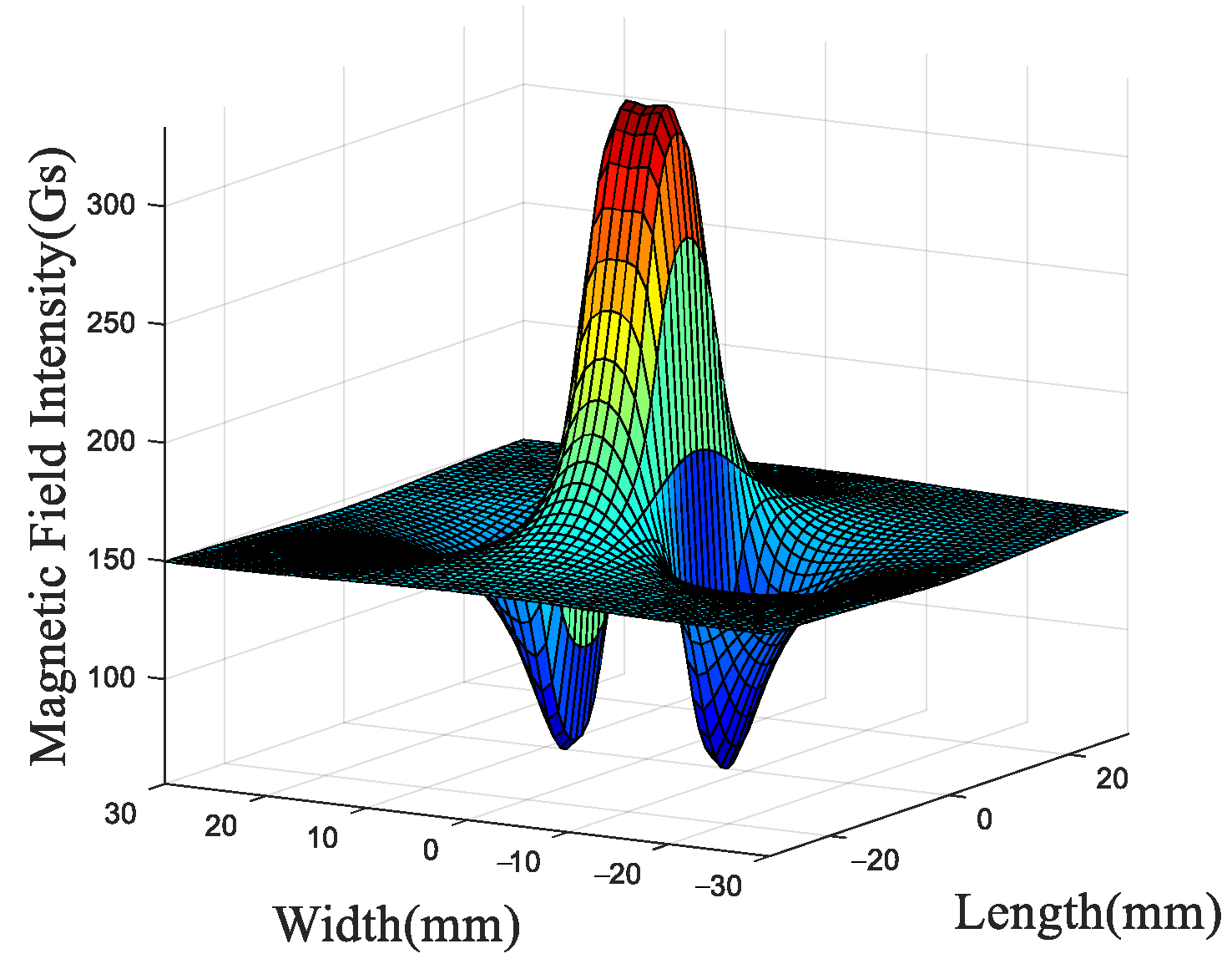
The axial MFL signal shown in Figure 5 reflects the spatial variation in the axial magnetic field component distributed along the x-direction and z-direction, providing key information about defect-induced magnetic perturbations. As the difference between the measured and the estimated decreases, the constructed profile becomes closer to the actual defect.

Figure 5.
Axial MFL signal.
To achieve higher accuracy in defect inversion, this paper proposed the continuity correction strategy and a hybrid CO-DE-SBOA, which are introduced in the following section.
3. Inversion Algorithm
3.1. Inversion Based on CO-DE-SBOA
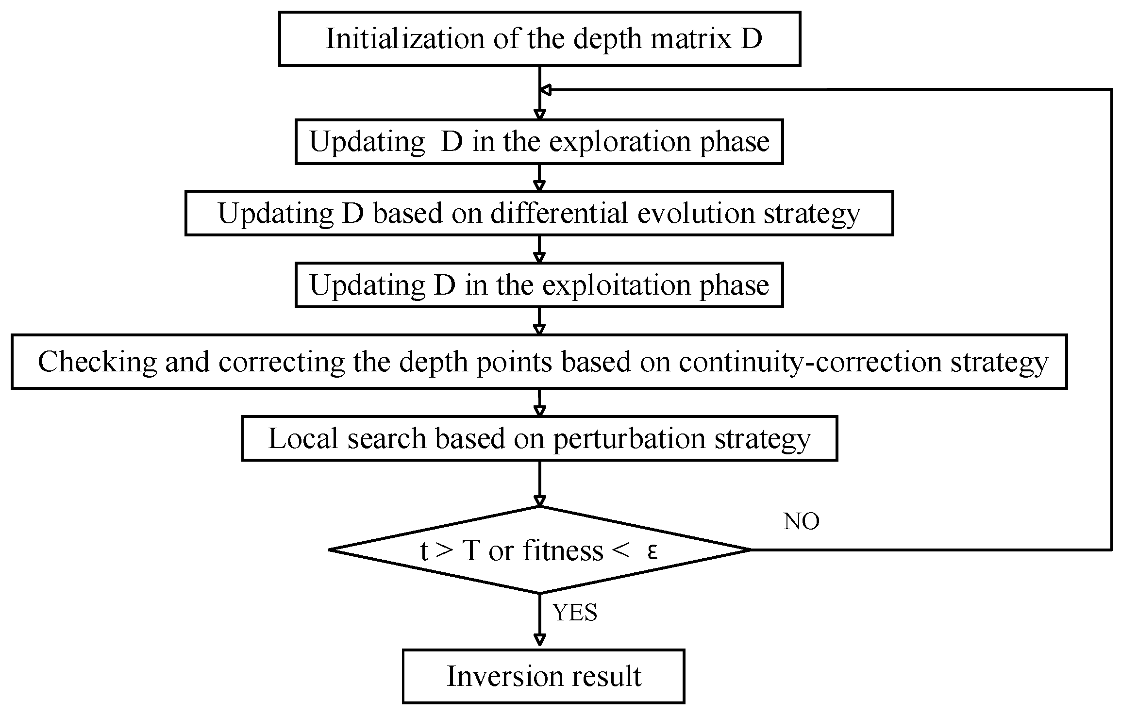
The process of the proposed CO-DE-SBOA is shown in Figure 6. At the beginning, the depth matrices need to be initialized. In each iteration, the depth matrices are updated based on the exploration phase of SBOA, differential evolution strategy, and exploitation phase of SBOA sequentially. Then, the method checks the depth values in the current iteration and adjusts the implausible points based on the proposed continuity correction strategy. Finally, the depth values are optimized through the perturbation strategy. When the fitness function is less than a certain value or the maximum number of iterations is reached, the iteration stops and the results are returned.
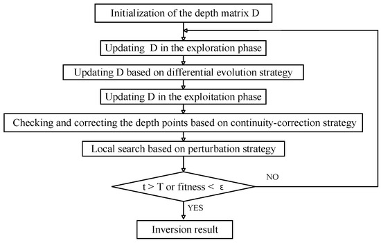
Figure 6.
Process of CO-DE-SBOA.
3.2. Continuity Correction (CO) Strategy
In the MFL-based inversion process, the algorithm searches for the optimal solution by minimizing the fitness. In the paper, the fitness function is the sum of squared errors between the predicted signal and the measured signal :
However, the difference between and does not completely reflect the difference between the constructed profile and the actual defect. In addition to optimizing the fitness, the plausibility of the solution should also be examined to ensure consistency with the actual defect characteristics.
During actual measurement, the material composition and structural design of the pipeline segment are the same. And, most defects in pipelines are caused by corrosion, abrasion, and localized deformation, which are typically progressive and lead to relatively continuous changes in depth. Therefore, the depth value of one defect cannot deviate excessively from the surrounding depth points. Based on the relative geometric continuity of depth values within the defect, this paper proposed a continuity correction (CO) strategy to adjust the implausible depth values and optimize the inversion process.
In the iterative process, each depth point should be examined, whether it deviates excessively from the surrounding points. The set of depth values {} in the neighborhood of the depth point (i,j) is denoted as . The average of the absolute values of the difference between the depth value and values in should be compared with a maximum allowable value . If satisfies (3),
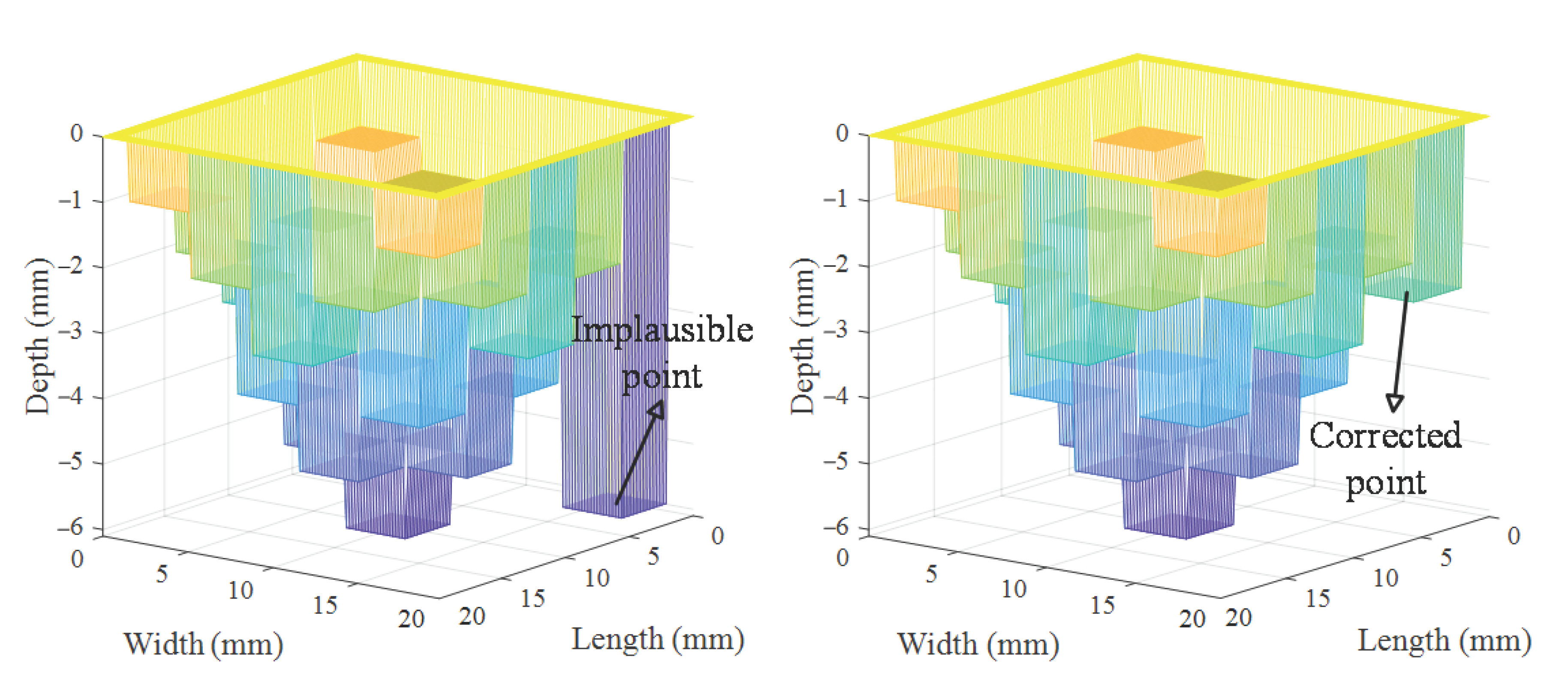
it is considered to be an implausible point (as shown in Figure 7a), which needs to be adjusted to to establish continuity with surrounding points:

Figure 7.
Correction of error points. (a) Implausible point. (b) Corrected point.
The adjusted solution needs to be compared with . If , . The adjustment helps the inversion process shift away from the local optima, and the adjusted would better align with actual defects (as shown in Figure 7b). To ensure the effectiveness of this strategy, the is adjusted dynamically based on the pipeline thickness d and the number of iterations:
where n is the number of segments of the defect along the length or the width. is the maximum variation. d/(n − 1) represents the baseline reference. represents the variation in the constraint. In the early stages of iteration, takes a smaller value to enhance convergence. In the later stages, takes a larger value to improve the inversion accuracy at the deeper points. The strategy effectively avoids persistent local optima in the inversion process and improves inversion accuracy.
3.3. Secretary Bird Optimization Algorithm (SBOA)
SBOA is a novel population-based metaheuristic algorithm based on the survival behavior of secretary birds. SBOA is divided into three phases: the initiation phase, the exploration phase, and the exploitation phase.
The initiation phase: Given the upper bound and lower bound for each dimension, N initial solutions are generated uniformly within the range between the bounds. And, N solutions form the population matrix . Each solution corresponds to a fitness .
The exploration phase: In this phase, the new solution varies with the iteration number t:
where T is the maximum number of iterations. and are random solutions from the current population. , and . is the current optimal solution. is the Levy flight step:
where Levy(Dim) is the Levy flight distribution function:
where s and are parameters. u and v are random numbers from the interval [0, 1]. Γ is the gamma function. If , .
The exploitation phase: In this phase, the new solution is generated with two strategies:
where R is a random number from the interval [0, 1]. is a parameter. , and . . is a randomly selected solution from the current population. When , .
3.4. Differential Evolution and Perturbation
SBOA has a strong search capability. But, when SBOA is used in 3-D defect profile inversion, it has less information exchange within its populations. To address this issue, the differential evolution (DE) strategy is placed between the exploration phase and the exploitation phase. It can improve the information exchange among solutions in the population. And, it can also broaden the search space. The strategy consists of a mutation process and a crossover process. The formula for mutant solution is as follows:
where is a random number from the interval [0, 1]. is a parameter. , and are different randomly selected solutions from . The formula for the adaptive mutant factor F is as follows:
where and are random numbers from the interval [0, 1]. is a parameter. , , and are mutant parameters. is constrained to be between and . is used in the crossover process to calculate the experimental solution:
where is a random number from the interval [0, 1]. CR is the crossover rate. If , .
Additionally, to further improve the solution by exploring its neighborhood, a perturbation strategy is placed after the exploitation phase. The updating formula is as follows:
where p is the perturbation rate. . is confined between and . If , .
3.5. Parameter Analysis
The parameters used are shown in Table 1. The parameters are mainly divided into three categories. The first category has little effect on the algorithm performance and is usually assigned directly based on human experience. s and are parameters which are related to the Levy flight. and are assigned to make the possibilities of each strategy equal. , , and are related to the differential evolution strategy. The second type of parameter is mainly related to experimental calculations, including N, T, d, and . These parameters have little impact on the algorithm itself and are determined based on experimental experience. The third category has important influence on the algorithm, including CR, p, and . These parameters are optimized through a univariate grid search. CR is the crossover rate, which is set to a larger value to expand the search space. p is the perturbation rate, which is set to a smaller value to ensure the stability of the solutions in each generation. is the maximum variation in , which should be set to a moderate value to meet the variation requirements of . An excessively large would cause the continuity correction strategy to perform unnecessary corrections in early iterations and fail to make effective corrections in later iterations. Conversely, an excessively small would make the variations in during the iteration process less effective.

Table 1.
Parameter values.
4. Experiment and Analysis
This section presents several experiments to demonstrate the superiority of the proposed CO-DE-SBOA. Section 4.1 introduces the experimental platform and the hardware conditions for performing the inversion. Section 4.2 describes the five metrics used to evaluate the algorithm. Section 4.3 compares the proposed algorithm with other algorithms, demonstrating its higher accuracy. Section 4.4 verifies the robustness of the method through the robustness experiment. Section 4.5 validates the effectiveness of each strategy in the proposed method through an ablation experiment.
4.1. Experimental Conditions
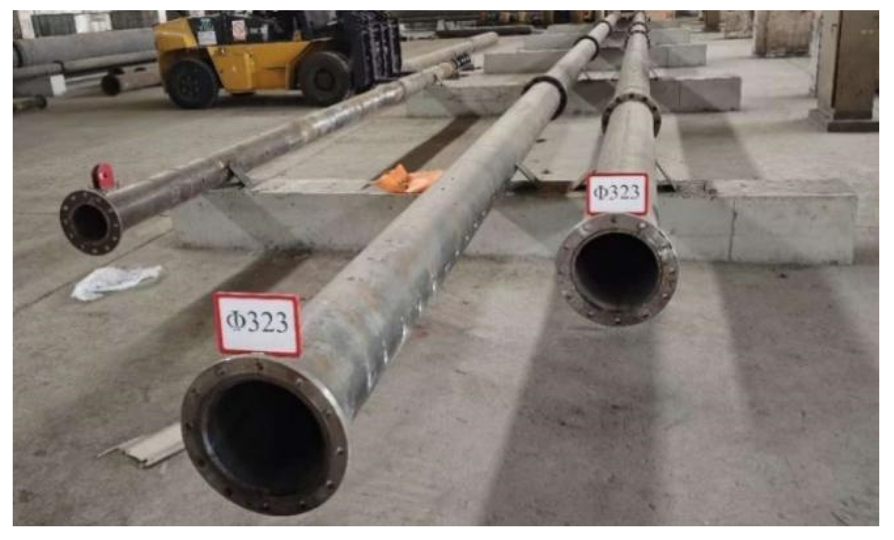
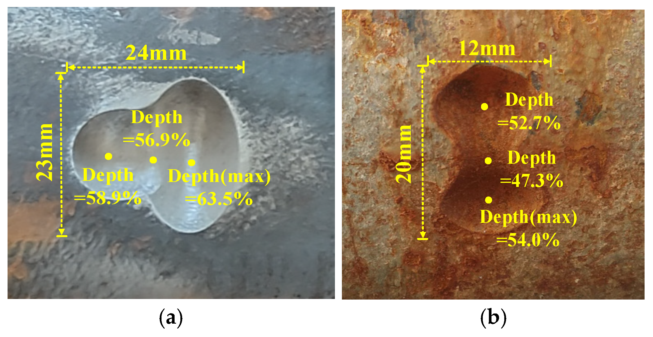
The experiments in this paper were conducted on the experimental platform (as shown in Figure 8) of a pipeline tensile testing facility in Shenyang. The total length of the pipeline on the experimental platform is over 30 m. The pipeline has a diameter of 323 mm and a thickness of 12.7 mm. Although the experiments were conducted on a pipe wall thickness of 12.7 mm, the proposed algorithm can also be applied to pipelines with smaller wall thicknesses, in which case the magnetization intensity should be reduced accordingly. During the experiment, the detector is pulled from one side to the other at a speed of 0.5 m/s. After the experiment, the stored data are retrieved and processed into signals suitable for defect profile inversion. Several collected defect samples are shown in Figure 9.

Figure 8.
Experimental platform.
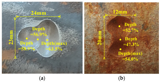
Figure 9.
Defect samples. (a) Sample I. (b) Sample II.
All experiments were implemented in MATLAB R2023(b) on a personal laptop with an Intel I7-12700H central processing unit and 16.00 GB of RAM.
4.2. Evaluation Metrics
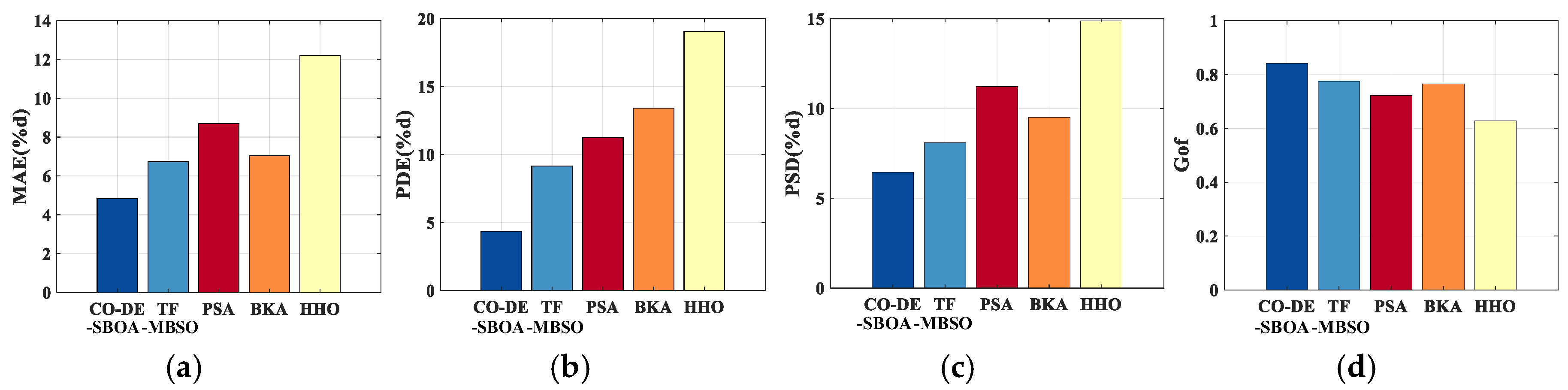
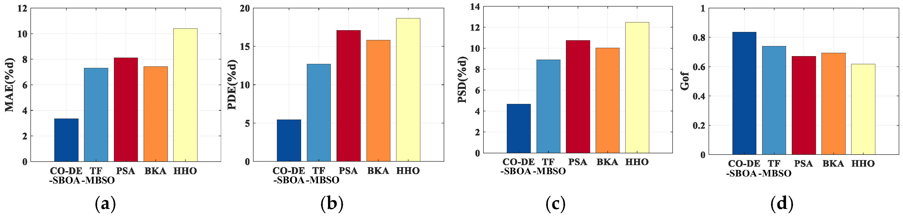
To validate the superior inversion accuracy of the proposed CO-DE-SBOA, it is compared with four other algorithms on five metrics. The compared algorithms are TF-MBSO, PSA, BKA, and HHO. The five metrics are mean absolute error (MAE), peak depth error (PDE), profile standard deviation (PSD), goodness of fit (Gof), and standard deviation (STD). MAE reflects the overall accuracy of the algorithm. PDE reflects the accuracy at the deepest point, affecting the profile’s size and shape. PSD and Gof reflect the fitting ability of the algorithm. STD reflects the stability of the algorithm. The formulas for these metrics are as follows:
where and represent the inverted values and actual values at each depth point. The actual values are selected from the geometric center of each segmented region by 3-D laser scanning. is the number of depth points in each defect, which is 5 5 in this paper. and represent each metric above and its average value. represents the number of inversion experiments conducted for each defect. In the experiment, N = 100 and T = 90.
4.3. Accuracy Experiment
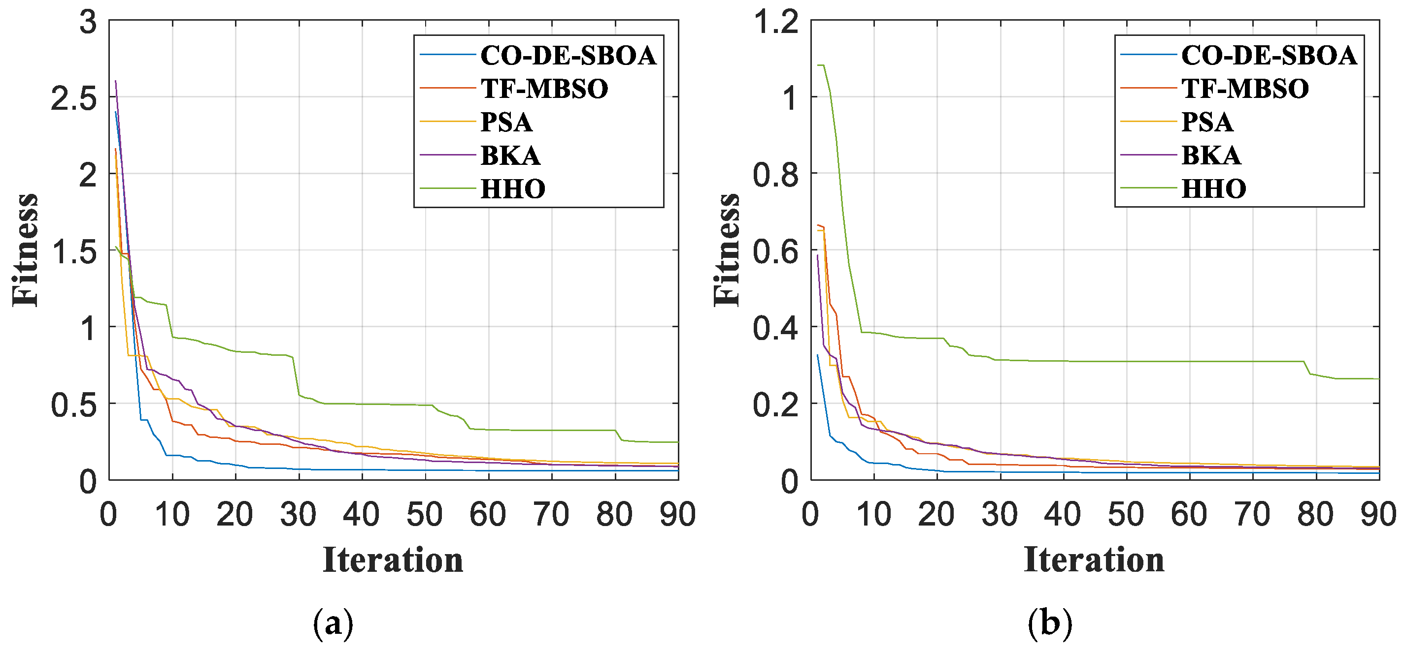
Taking the defects in Figure 9 as an example, the iteration curves are shown in Figure 10. Among the methods, CO-DE-SBOA exhibits the strongest convergence ability, reducing the fitness to a lower value within 20 generations in the experiments with two samples. Then, TF-MBSO converges relatively quickly. PSA and BKA exhibit similar convergence abilities, requiring more iterations to minimize the fitness. HHO exhibited poor convergence abilities, failing to achieve convergence. The comparison proved the strong convergence ability of CO-DE-SBOA.
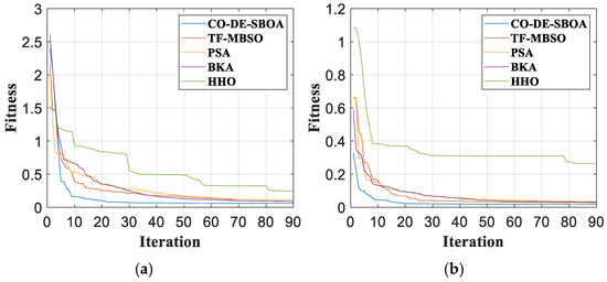
Figure 10.
Fitness curves. (a) For sample I. (b) For sample II.
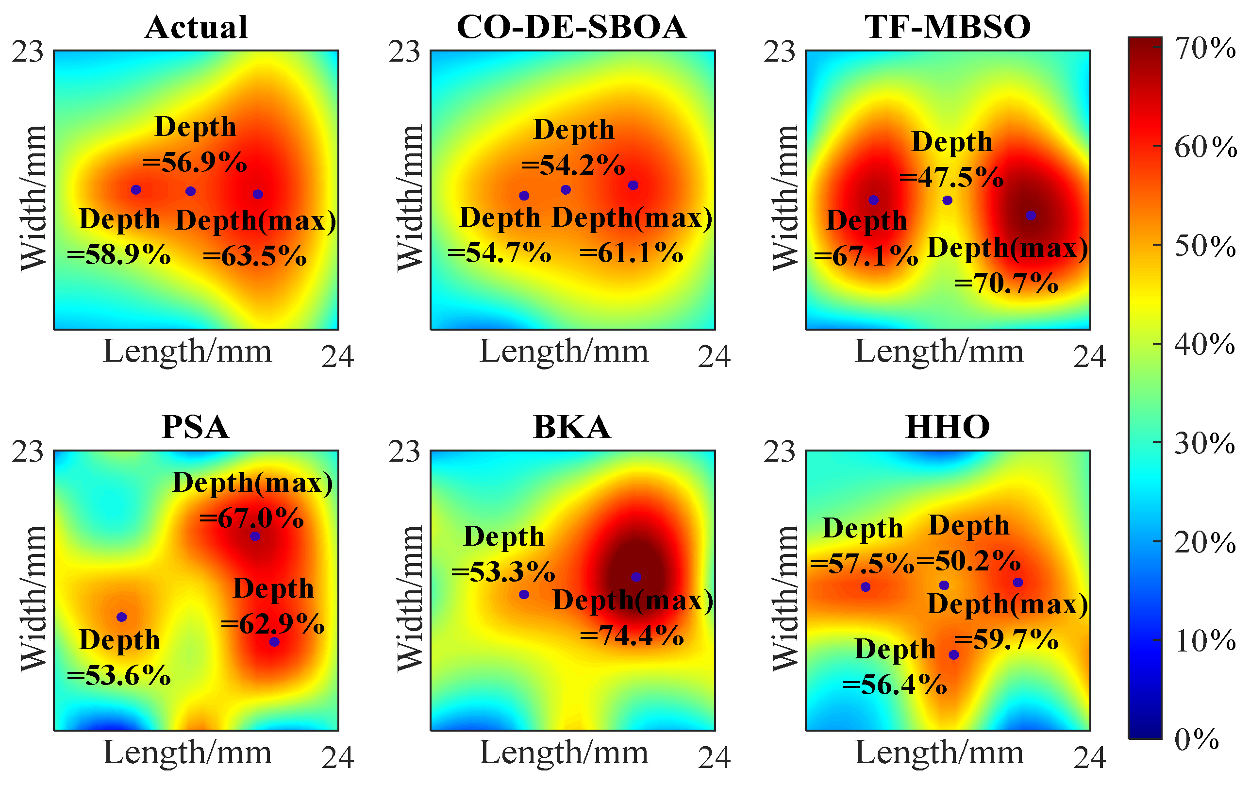
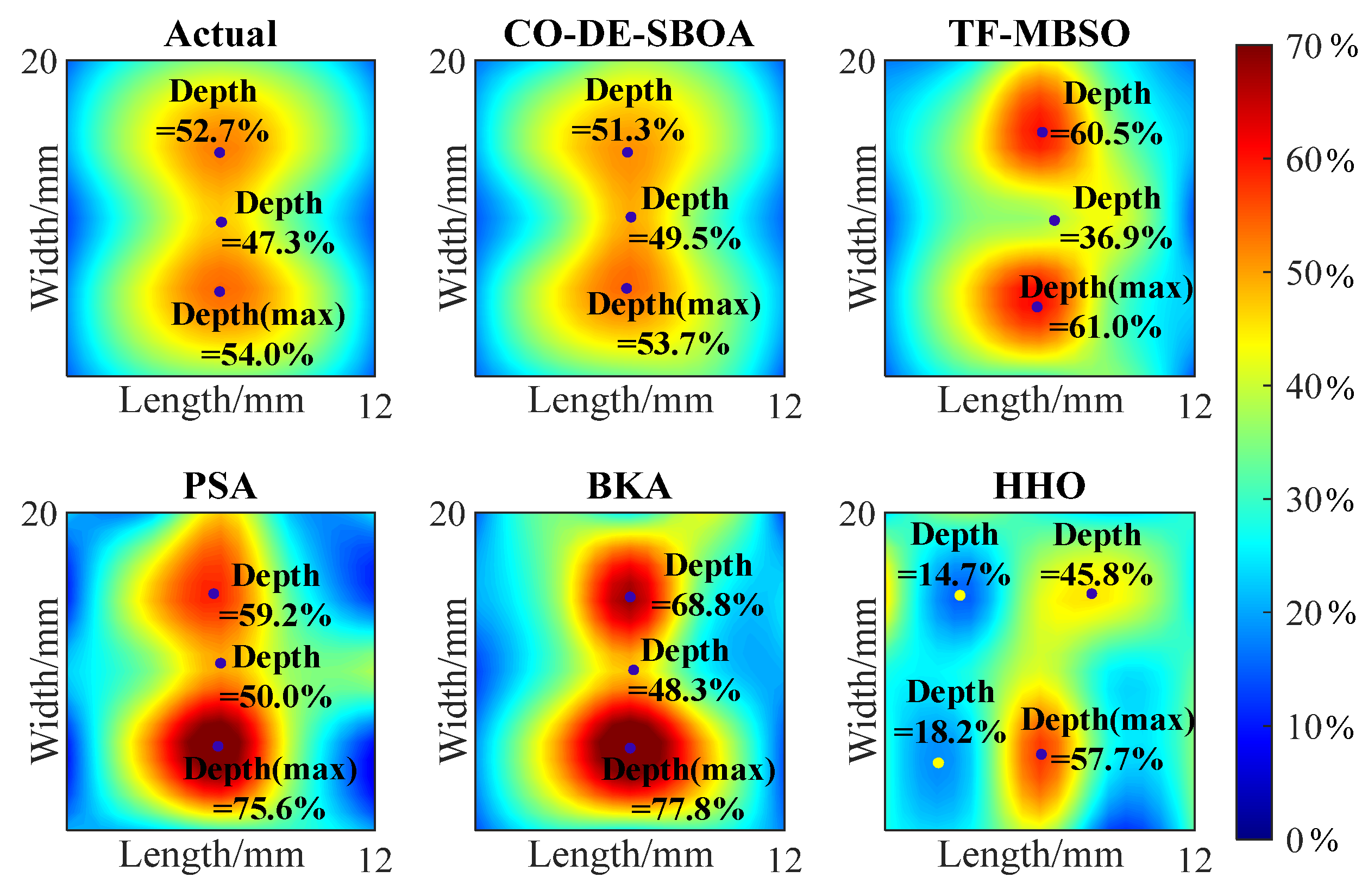
The 5 5 depth matrices obtained from the inversion are represented as heat maps and compared with the heat maps of actual defects, as shown in Figure 11 and Figure 12. The comparison shows that CO-DE-SBOA can reconstruct the defect’s profile with higher accuracy. TF-MBSO can highlight deeper points, but the errors in the specific values are relatively large. PSA and BKA exhibited moderate fitting abilities, but their depth values deviated from the defects. In contrast, HHO exhibited limited fitting capabilities, limiting defect profile reconstruction. For the estimation of the deepest point and key points affecting the defects’ shapes, CO-DE-SBOA achieved smaller deviations from the actual defects, while PSA and BKA produced larger estimation errors at these points. The comparison proved the strong profile fitting capability of CO-DE-SBOA.
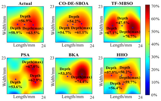
Figure 11.
Heat map of the depth matrix of sample I.
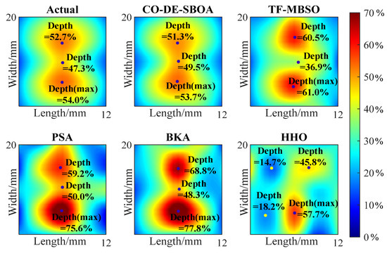
Figure 12.
Heat map of the depth matrix of sample II.
The inversion metrics for the two defect samples, using five methods over 30 trials, are shown in Figure 13 and Figure 14. Among them, CO-DE-SBOA showed the smallest error across the metrics.
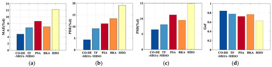
Figure 13.
Accuracy comparison of sample I. (a) MAE. (b) PDE. (c) PSD. (d) Gof.

Figure 14.
Accuracy comparison of sample II. (a) MAE. (b) PDE. (c) PSD. (d) Gof.
To further validate the accuracy of CO-DE-SBOA, the MFL signals from 50 defects were measured. For each MFL signal, 30 inversions were conducted using the five methods above. The average values of metrics were compared in Table 2. The comparison results indicate that the CO-DE-SBOA outperforms the other four algorithms across all metrics, with MAE and PDE both under 5%. The method’s superiority in MAE reflects its overall higher inversion accuracy. Its superiority in PDE enables more accurate estimation of the defect’s size and shape. PSD and Gof reflect its superior profile fitting ability. Its smaller values in STD compared to other algorithms reflect the method’s stability.
Table 2.
Accuracy Experiment.
According to the specifications and requirements for the intelligent pig inspection of pipelines written by the pipeline operators forum (POF) [26], the inversion results should be evaluated using confidence levels. We sorted the PDE of the above sample experiments, counted the number of times the PDE accuracy index of each algorithm was lower than 10%, and calculated the confidence level based on this, as shown in Table 3. The results indicate that the confidence level of CO-DE-SBOA is 95% when PDE < 10%, which is higher than that of other methods.
Table 3.
Certainty level.
From the experimental results, it can be concluded that the inversion accuracy of this method is superior to conventional algorithms. However, when dealing with defects with higher complexity, a 5 × 5 depth matrix is insufficient to restore all defect details. In addition, pipelines are often equipped with “Ω-shaped” expansion compensators [27], where the corners tend to exhibit stress concentration, defect accumulation, and structural variations. The proposed method is applicable to both straight sections and corner regions of the pipeline, although the inversion accuracy may decline in the latter due to increased geometric complexity. Because the defect inversion process can be completed in the off-line condition, the higher accuracy of the method has significant practical implications.
4.4. Robustness Experiment
To verify the robustness of CO-DE-SBOA in measurements under interference, 5% and 10% Gaussian noise were added to the 50 measured signals, with each processed signal undergoing 30 inversions. The results are shown in Table 4.
Table 4.
Robustness experiment.
When the noise level increases from 0% to 10%, the increments in MAE, PDE, and PSD are 2.1%, 1.9%, and 2.3%, with a minimal change in standard deviation (STD). The results demonstrate the robustness of the proposed CO-DE-SBOA.
4.5. Ablation Experiment
To validate that all components of our method contribute to the results, an ablation experiment was conducted. Because of the superior search capability of SBOA, the ablation experiment used SBOA as the main algorithm, with differential evolution, perturbation, and continuity correction as optimization strategies. For the combinations of different strategies in our method, the same defect samples with MFL signals were used for the inversion experiments. The combinations of strategies and their results are shown in Table 5.
Table 5.
Ablation experiment.
For the experiments in which continuity correction was removed, shown in the first four rows of Table 5, relatively poor performance can be concluded. Especially when SBOA was applied alone, with the average PDE exceeding 10%, which can lead to significant errors in profile construction. On this basis, differential evolution and perturbation were applied separately with SBOA, resulting in different degrees of improvement. Among these, differential evolution demonstrated relatively greater improvement across various metrics, highlighting its effectiveness in enhancing the algorithm’s search capability.
From the last four rows in Table 5, it can be concluded that the use of continuity correction significantly improves the accuracy of the results. Notably, continuity correction lowered the PDE by 6% across various strategy combinations, bringing the average value below 5%. The optimization of PDE reflects its improvement of the accuracy at deeper points. And, the optimization of MAE, PSD, and Gof reflects the improvements in overall accuracy and fitting capability. On this basis, differential evolution and perturbation individually optimized each metric, and their combined application produced superior results. It improved the accuracy, fitting capability, and stability of the method through all the proposed strategies.
5. Conclusions
Three-dimensional defect profile inversion with higher degrees of freedom is of great significance for accurate defect assessment. In order to overcome the limitations of low accuracy and insufficient robustness in existing inversion algorithms, this paper proposes a strategy which examines the value of each depth point and corrects implausible points based on the geometric continuity of defects. On this basis, this paper proposes the CO-DE-SBOA, which integrates SBOA and the differential evolution strategy to improve the global search capability. The accuracy experiments demonstrate that the proposed method outperforms existing methods, reducing the MAE and PDE by 3.6% and 7.1%, respectively.
In the robustness experiments with 10% noise added, MAE and PDE increased by only 2.1% and 1.9%, demonstrating the superior robustness of the algorithm. Additionally, excessively complex defect profiles rely on higher-degree-of-freedom inversion for accurate reconstruction. In future research, the method in this paper will provide a reference for the defect inversion of a higher degree of freedom.
Author Contributions
Conceptualization, C.W. and S.L.; Formal analysis, Y.D.; Investigation, J.T.; Methodology, C.W. and S.L.; Resources, S.L.; Software, C.W.; Validation, J.T. and Y.D.; Writing—original draft, C.W. and H.W.; Writing—review and editing, C.W. and S.L. All authors have read and agreed to the published version of the manuscript.
Funding
This research was funded by the National Natural Science Foundation of China (grant No U22A2055 and grant No 62273058).
Institutional Review Board Statement
Not applicable.
Informed Consent Statement
Not applicable.
Data Availability Statement
The data that support the findings of this study are available from the corresponding author Senxiang Lu upon reasonable request.
Conflicts of Interest
Author Jianhua Tang was employed by the company CNOOC EnerTech-Equipment Technology Co., Ltd. The remaining authors declare that the research was conducted in the absence of any commercial or financial relationships that could be construed as a potential conflict of interest.
Nomenclature
| Matrix of measured MFL signals | |
| Matrix of inverted MFL signals | |
| Depth value of depth point (i,j) | |
| Magnetic field distribution corresponding to depth point (i,j) | |
| Matrix of depth values | |
| n | Number of divisions per dimension of the defect |
| m | Number of sampling points along each dimension |
| Set of depth values of the depth points adjacent to depth point (i,j) | |
| Depth value of the depth point adjacent to depth point (i,j) | |
| Maximum allowable value of the continuity correction strategy | |
| Maximum variation in the continuity correction strategy | |
| Maximum number of iterations | |
| N | Number of secretary bird individuals |
| Upper bound of the initial solution | |
| Lower bound of the initial solution | |
| d | Thickness of the pipe wall |
| Dim | Dimension of the solution |
| s | Parameter related to Lévy flight |
| Parameter related to Lévy flight | |
| F | Adaptive mutant factor |
| Variation value of the dynamic mutation parameter | |
| Reference value of the dynamic mutation parameter | |
| Static mutation parameter | |
| Crossover rate | |
| p | Perturbation rate |
| Iteration stopping threshold | |
| Number of depth points in each defect | |
| Number of inversion experiments conducted for each defect | |
| Each error metric | |
| Average value of the error metric |
References
- Lu, S.; Zhou, T.; Wang, C.; Lin, Z.; Yi, G. An internal detector positioning method in oil pipelines using vibration signal. IEEE Sens. J. 2023, 23, 13411–13421. [Google Scholar] [CrossRef]
- Ma, Q.; Tian, G.; Zeng, Y.; Li, R.; Song, H.; Wang, Z.; Gao, B.; Zeng, K. Pipeline In-Line Inspection Method, Instrumentation and Data Management. Sensors 2021, 21, 3862. [Google Scholar] [CrossRef] [PubMed]
- Shi, Y.; Zhang, C.; Li, R.; Cai, M.; Jia, G. Theory and Application of Magnetic Flux Leakage Pipeline Detection. Sensors 2015, 15, 31036–31055. [Google Scholar] [CrossRef]
- Yu, G.; Liu, J.; Zhang, H.; Liu, C. An iterative stacking method for pipeline defect inversion with complex MFL signals. IEEE Trans. Instrum. Meas. 2019, 69, 3780–3788. [Google Scholar] [CrossRef]
- Wu, Z.; Deng, Y.; Liu, J.; Wang, L. A reinforcement learning-based reconstruction method for complex defect profiles in MFL inspection. IEEE Trans. Instrum. Meas. 2021, 70, 2506010. [Google Scholar] [CrossRef]
- Liu, J.; Shen, X.; Wang, J.; Jiang, L.; Zhang, H. An intelligent defect detection approach based on cascade attention network under complex magnetic flux leakage signals. IEEE Trans. Ind. Electron. 2022, 70, 7417–7427. [Google Scholar] [CrossRef]
- Yuksel, V.; Tetik, Y.E.; Basturk, M.O.; Recepoglu, O.; Gokce, K.; Cimen, M.A. A novel cascaded deep learning model for the detection and quantification of defects in pipelines via magnetic flux leakage signals. IEEE Trans. Instrum. Meas. 2023, 72, 2512709. [Google Scholar] [CrossRef]
- Khodayari-Rostamabad, A.; Reilly, J.P.; Nikolova, N.K.; Hare, J.R.; Pasha, S. Machine Learning Techniques for the Analysis of Magnetic Flux Leakage Images in Pipeline Inspection. IEEE Trans. Magn. 2009, 45, 3073–3084. [Google Scholar] [CrossRef]
- Pasadas, D.J.; Baskaran, P.; Ramos, H.G.; Ribeiro, A.L. Detection and Classification of Defects Using ECT and Multi-Level SVM Model. IEEE Sens. J. 2020, 20, 2329–2338. [Google Scholar] [CrossRef]
- Feng, B.; Wu, J.; Tu, H.; Tang, J.; Kang, Y. A Review of Magnetic Flux Leakage Nondestructive Testing. Materials 2022, 15, 7362. [Google Scholar] [CrossRef]
- Zhang, S.; Li, H.; Zhao, C. Magnetic-charge element method for magnetic flux leakage inspection. IEEE Trans. Instrum. Meas. 2022, 71, 6007910. [Google Scholar] [CrossRef]
- Gao, P.; Geng, H.; Yang, L.; Su, Y. Research on the Forward Solving Method of Defect Leakage Signal Based on the Non-Uniform Magnetic Charge Model. Sensors 2023, 23, 6221. [Google Scholar] [CrossRef]
- Liu, B.; Lian, Z.; Liu, T.; Wu, Z.; Ge, Q. Study of MFL signal identification in pipelines based on non-uniform magnetic charge distribution patterns. Meas. Sci. Technol. 2023, 34, 044003. [Google Scholar] [CrossRef]
- Amineh, R.K.; Koziel, S.; Nikolova, N.K.; Bandler, J.W.; Reilly, J.P. A Space Mapping Methodology for Defect Characterization From Magnetic Flux Leakage Measurements. IEEE Trans. Magn. 2008, 44, 2058–2065. [Google Scholar] [CrossRef]
- Priewald, R.H.; Magele, C.; Ledger, P.D.; Pearson, N.R.; Mason, J.S.D. Fast Magnetic Flux Leakage Signal Inversion for the Reconstruction of Arbitrary Defect Profiles in Steel Using Finite Elements. IEEE Trans. Magn. 2013, 49, 506–516. [Google Scholar] [CrossRef]
- Han, W.; Xu, J.; Zhou, M.; Tian, G.; Wang, P.; Shen, X.; Hou, E. Cuckoo search and particle filter-based inversing approach to estimating defects via magnetic flux leakage signals. IEEE Trans. Magn. 2015, 52, 6200511. [Google Scholar] [CrossRef]
- Lu, S.; Feng, J.; Li, F.; Liu, J. Precise inversion for the reconstruction of arbitrary defect profiles considering velocity effect in magnetic flux leakage testing. IEEE Trans. Magn. 2016, 53, 6201012. [Google Scholar] [CrossRef]
- Lu, S.; Liu, J.; Wu, J.; Fu, X. A Fast Globally Convergent Particle Swarm Optimization for Defect Profile Inversion Using MFL Detector. Machines 2022, 10, 1091. [Google Scholar] [CrossRef]
- Li, F.; Feng, J.; Zhang, H.; Liu, J.; Lu, S.; Ma, D. Quick reconstruction of arbitrary pipeline defect profiles from MFL measurements employing modified harmony search algorithm. IEEE Trans. Instrum. Meas. 2018, 67, 2200–2213. [Google Scholar] [CrossRef]
- Hou, D.; Lu, S.; Yi, G.; Qiu, J.; Liu, J. A Target-Focusing Optimization Method for 3D Profile Reconstruction of Defects using MFL Measurements. IEEE Trans. Instrum. Meas. 2023, 21, 2521911. [Google Scholar]
- Zhao, J.; Zhang, M.; Zhao, B.; Du, X.; Zhang, H.; Shang, L.; Wang, C. Integrated Reactive Power Optimisation for Power Grids Containing Large-Scale Wind Power Based on Improved HHO Algorithm. Sustainability 2023, 15, 12962. [Google Scholar] [CrossRef]
- Li, B.; Yang, J. A modified whale optimization algorithm for electromagnetic inverse problems. In Proceedings of the 2020 IEEE 1st China International Youth Conference on Electrical Engineering (CIYCEE), Wuhan, China, 1–4 November 2020; pp. 1–7. [Google Scholar]
- Gao, Y. PID-based search algorithm: A novel metaheuristic algorithm based on PID algorithm. Expert Syst. Appl. 2020, 232, 120886. [Google Scholar] [CrossRef]
- Fu, Y.; Liu, D.; Chen, J.; He, L. Secretary bird optimization algorithm: A new metaheuristic for solving global optimization problems. Artif. Intell. Rev 2024, 57, 123. [Google Scholar] [CrossRef]
- Wang, J.; Wang, W.C.; Hu, X.X.; Qiu, L.; Zang, H.F. Black-winged kite algorithm: A nature-inspired meta-heuristic for solving benchmark functions and engineering problems. Artif. Intell. Rev. 2024, 57, 98. [Google Scholar] [CrossRef]
- Pipeline Operators Forum. POF 100: Specifications and Requirements for In-Line Inspection of Pipelines. 2021. Available online: https://pipelineoperators.org/documents (accessed on 18 May 2025).
- Banaszek, A.; Łosiewicz, Z.; Jurczak, W. Corrosion influence on safety of hydraulic pipelines installed on decks of contemporary product and chemical tankers. Pol. Marit. Res. 2018, 25, 71–77. [Google Scholar] [CrossRef]
Disclaimer/Publisher’s Note: The statements, opinions and data contained in all publications are solely those of the individual author(s) and contributor(s) and not of MDPI and/or the editor(s). MDPI and/or the editor(s) disclaim responsibility for any injury to people or property resulting from any ideas, methods, instructions or products referred to in the content. |
© 2025 by the authors. Licensee MDPI, Basel, Switzerland. This article is an open access article distributed under the terms and conditions of the Creative Commons Attribution (CC BY) license (https://creativecommons.org/licenses/by/4.0/).