Analytical Regression and Geometric Validation of the Blade Arc Segment $\stackrel{⌢}{\mathrm{BC}}$ in a Michell–Banki Turbine

Abstract

This study introduces a systematic methodology for modelling the radius of curvature of the arc-shaped section $\stackrel{⌢}{\mathrm{BC}}$ in a Michell–Banki cross-flow turbine blade. The method combines geometric modeling in polar coordinates with nonlinear regression, using both two- and three-parameter formulations estimated through the Ordinary Least Squares (OLS) method. Model performance is assessed through two complementary criteria: the coefficient of determination ($R^2$) and the computed arc length, ensuring that statistical accuracy aligns with geometric fidelity. The methodology was validated on digital measurements obtained from CATIA, using datasets with $N=187$ and a reduced subset of $N=48$ points. Results demonstrate that even with fewer data points, the regression model maintains high predictive accuracy and geometric consistency. The best-performing three-parameter model achieved $R^2=0.958$, with a five-point Gauss–Legendre quadrature yielding an arc length of approximately $145\mathrm{mm}$, representing 98.8% agreement with the reference value of $146.78\mathrm{mm}$. By representing the arc as a single smooth exponential function rather than a piecewise mapping, the approach simplifies analysis and enhances reproducibility. Coupling regression precision with arc-length verification provides a robust and reproducible basis for curvature modeling. This methodology supports turbine blade design, manufacturing, and quality control by ensuring that the blade geometry is validated with high statistical confidence and physical accuracy. Future research will focus on deriving analytical arc-length integrals and integrating the procedure into automated design and inspection workflows.

1. Introduction

The geometric and statistical analysis of a turbine blade’s surface profile plays a critical role in optimizing the design, fabrication, and operational performance of cross-flow turbines. This study focuses on the curved section $\stackrel{⌢}{\mathrm{BC}}$ of a Michell–Banki-type turbine blade [1,2,3]. Accurate modeling of the blade’s geometry is essential for predicting flow behavior, assessing manufacturing precision, and ensuring efficient energy transfer. To achieve this, we employ a nonlinear regression formulation that provides a compact analytical representation of the blade profile, allowing explicit evaluation of geometric fidelity, statistical measures, and predictive robustness. This approach enables direct estimation of critical features such as curvature and arc length, supporting design validation and quality control.

The study begins with a detailed description of section $\stackrel{⌢}{\mathrm{BC}}$, including coordinate systems and geometric sampling methodology. A 3D model and precise sampling were carried out in CATIA V5R21 [4], enabling accurate extraction of geometric coordinates. Nonlinear regression models using the Least Squares Method (LSM/OLS) are developed, with clear exposition of the mathematical framework, assumptions, and statistical validation metrics [5,6,7,8].

Two- and three-parameter regression models are examined, with statistical validity assessed through the coefficient of determination ($R^2$), residual analysis, and cross-validation to avoid overfitting. The three-parameter model in particular resolves limitations observed in the two-parameter model, providing a closer fit to the measured points while preserving geometric fidelity. Subset analysis with reduced data density ($N=48$ of $N=187$) demonstrates model robustness under different measurement strategies, highlighting the method’s applicability even with limited observations.

The arc length of $\stackrel{⌢}{\mathrm{BC}}$ is computed using the regression models combined with Gauss–Legendre quadrature integration [9,10]. The resulting measurements closely match the original reference values, confirming that this modeling approach offers both precision and reliability in design validation and quality control of micro-hydro turbine blades [11,12].

Previous studies have emphasised the sensitivity of turbine performance and manufacturability to blade geometry. For instance, 3D-CFD analyses of tidal Hunter turbines have shown that variations in stroke angles and the addition of winglets can substantially modify the power coefficient [13]. Similarly, recent reviews on the manufacturing of integrally bladed rotors (IBRs) highlight the geometric complexity and precision requirements of turbomachinery components [14]. These investigations collectively demonstrate that blade geometry is a critical determinant of efficiency and quality. The present study contributes to this research line by offering a geometrically rigorous and statistically validated analytical model of the curved segment $\stackrel{⌢}{\mathrm{BC}}$, providing a reproducible procedure for design verification and manufacturing control in cross-flow turbines.

The novelty of this study lies in establishing a unified geometric–statistical approach for accurately modelling the curved section $\stackrel{⌢}{\mathrm{BC}}$ of a Michell–Banki turbine blade. Unlike previous works focused on fluid-dynamic optimisation or manufacturing techniques, the present approach introduces a compact nonlinear regression formulation that analytically reconstructs the blade profile from reference coordinates and enables direct computation of curvature and arc length through numerical integration. This integration of geometric modelling with statistical validation represents a distinct methodological contribution, providing a reproducible and quantitatively robust tool for design verification, dimensional analysis, and quality control in micro-hydro turbine blades.

2. Description of Curve of Section $\stackrel{⌢}{\mathrm{BC}}$ of a Cross Flow Turbine of Type Michell–Banki

This section provides a detailed geometric description of the blade’s surface profile in a cross-flow turbine, focusing on the curved segment denoted as $\stackrel{⌢}{\mathrm{BC}}$ (Figure 1). This segment is of particular interest because its curvature strongly affects the efficiency of energy transfer within the turbine.

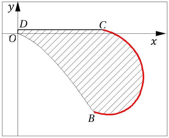
Figure 1. Section $\stackrel{⌢}{\mathrm{BC}}$ (in red) of the blade’s superficial profile, modeled in CATIA. The horizontal and vertical axes are denoted by x and y, respectively [1].

Our focus in this study is primarily on the design and quality control aspects of the blade, rather than on detailed physical fluid dynamics. Accurately representing the geometry of $\stackrel{⌢}{\mathrm{BC}}$ is essential for verifying manufacturing precision, optimizing design parameters, and ensuring reproducible inspection protocols [15,16].

2.1. Physical and Geometric Context

The blade section $\stackrel{⌢}{\mathrm{BC}}$ is a key component of the Michell–Banki cross-flow turbine, as its curvature directly influences fluid flow patterns and the efficiency of energy transfer. Accurately determining the arc length and curvature of this segment is therefore relevant not only for geometric modeling but also for understanding the potential guidance of water along the blade, the angular momentum transfer, and the overall turbine performance.

To focus on geometric and manufacturing considerations, several simplifying assumptions are adopted: the blade is considered a rigid cast-iron component operating under steady-state conditions, with constant volumetric flow rate and temperature. These assumptions allow us to neglect thermodynamic effects, unsteady flows, and complex fluid-structure interactions, making it reasonable to treat the problem as primarily geometric. Under these conditions, the computed arc length serves as a reliable proxy for the blade’s physical role in the turbine, as it ensures the proper shape for energy transfer and flow guidance.

The nearly circular nature of the section and its radial curvature justify modeling the curve using polar coordinates and representing it as a single smooth function. This approach simplifies the computation of geometric quantities such as curvature and arc length, minimizes residual errors between measured and predicted coordinates, and provides a consistent framework for regression-based analysis. From a manufacturing and quality control perspective, this method enables straightforward verification of blade geometry, supports reproducible inspection, and facilitates parametric optimization during the design stage. By focusing on geometric fidelity under controlled physical assumptions, the mathematical representation of the curve can be directly linked to practical tasks such as production verification and design refinement.

2.2. Preliminary Observations

The section $\stackrel{⌢}{\mathrm{BC}}$ can be described using both polar and Cartesian coordinate systems [1], with Cartesian coordinates expressed in millimetres (mm) according to [3]. Geometric data were collected manually using a graduated ruler for linear distances (1 mm resolution) and a semicircular protractor for angular measurements (1° precision).

As a result, all sampled data points are effectively restricted to integer values, defining the achievable resolution and precision of the blade’s superficial profile representation. The 1 mm vertical offset in the CATIA model corresponds to the smallest resolution of the ruler, and the 1° increment in angular measurements reflects the precision limit of the protractor used during sampling.

The practical measurement resolution introduces quantifiable uncertainty in the data. The ruler precision ($\pm 1$ mm) corresponds to a standard deviation of approximately ${\sigma }_r=0.29$ mm, while the protractor precision ($\pm 1^{\circ }$) corresponds to ${\sigma }_{\theta }=0.005$ rad. Given the measurement domain of the section, with radii ranging from approximately 78 mm to 143 mm and angular positions spanning about ${44}^{\circ }$, these values correspond to relative uncertainties of roughly $0.8\%$ for linear distances and $2.3\%$ for angular measurements. These limits define the attainable precision of the sampled dataset and establish the expected range of measurement dispersion that will later be considered in the regression analysis.

2.3. Sampling Considerations

The sampling process for section $\stackrel{⌢}{\mathrm{BC}}$ is shaped by both the precision of the measuring tools and the requirement to preserve geometric continuity along the blade’s superficial profile (Figure 2). The angular position of point B is approximately $-{44}^{\circ }$, while point C is located at $3^{\circ }$. To ensure a consistent sampling resolution using 1-degree intervals, at least 48 distinct observations are required. Each observation corresponds to a unique radial distance (radius), and for analytical purposes, each is treated as an independent and identically distributed (i.i.d.) sample.

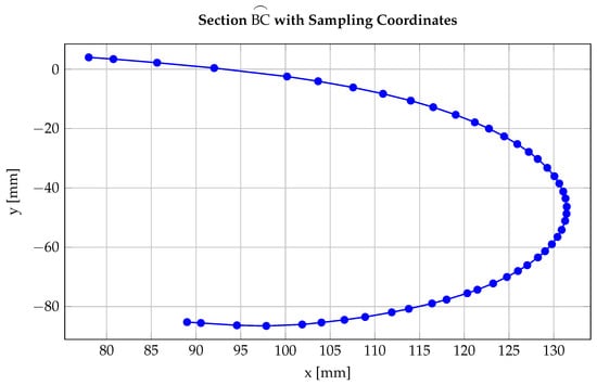
Figure 2. Section $\stackrel{⌢}{\mathrm{BC}}$ with coordinate samples spaced at 1-degree intervals (TikZ export).

Although any fixed pair of Cartesian coordinates could theoretically correspond to infinitely many polar angles, due to the continuous nature of real numbers, this ambiguity is circumvented by fixing the angular endpoints of the curve. The first and last sampled points (corresponding to the minimum and maximum angular positions) are preserved to ensure the continuity and geometric integrity of the blade’s superficial profile. This approach is justified by the physical constraints of the turbine blade and aligns with the modeling assumptions outlined in [1,3].

2.4. Methodology

Based on the geometric sampling framework described above, this study aims to determine an analytical model that accurately represents the arc shape of section $\stackrel{⌢}{\mathrm{BC}}$ and allows reliable computation of its arc length. The proposed methodology combines geometric modelling in polar coordinates with nonlinear regression techniques, providing a unified analytical description of the blade profile.

Two regression models were evaluated: a two-parameter and a three-parameter formulation, both fitted to the sampled data using the Ordinary Least Squares (OLS) method. Each model was assessed through two complementary criteria: (i) a minimum coefficient of determination of $R^2\ge 0.95$, ensuring high statistical accuracy, and (ii) an arc length ratio (predicted/measured) of at least 97%, ensuring geometric fidelity. Models expressed in polar coordinates were treated as a single smooth function $r\left(\theta \right)$, allowing consistent computation of curvature and arc length while minimizing residual errors between measured and predicted values.

The threshold $R^2\ge 0.95$ ensures that the regression model captures the majority of the variance in the sampled data, resulting in a statistically robust representation of the blade profile. The 97% arc length ratio guarantees that the geometric continuity and physical integrity of the curve are preserved, which is essential for maintaining correct flow guidance and energy transfer within the turbine.

From a practical standpoint, these criteria allow engineers to verify that manufactured blades adhere closely to the intended design using simple measurement tools such as rulers and protractors. In the design stage, such high-fidelity models enhance performance prediction and parameter optimisation, while in quality control, they support reproducible inspection and dimensional verification. Representing the entire arc as a single continuous function simplifies statistical evaluation, residual analysis, and arc-length integration, providing consistent and reliable results even with a reduced number of reference geometric observations.

It is important to note that the present analysis is based on geometric data extracted from the CATIA model of the Michell–Banki blade. This dataset represents the nominal design geometry and provides an ideal reference for developing and testing the analytical regression methodology under noise-free conditions. Although no direct measurements from manufactured blades were used, this does not affect the scope of the current work, which is focused on the mathematical validation of the modeling procedure. Future studies will extend the analysis to physical blade measurements obtained through coordinate or laser scanning, in order to evaluate the performance of the proposed regression framework under real manufacturing tolerances.

3. Regression Model Using LSM or OLS in Section $\stackrel{⌢}{\mathrm{BC}}$

The curvature of Section $\stackrel{⌢}{\mathrm{BC}}$ was modelled using the Ordinary Least Squares (OLS) method, which minimizes the sum of squared residuals between measured and predicted radii. This provides statistically optimal parameter estimates under standard assumptions of unbiasedness and constant variance. A full derivation of the OLS formulation and its application in polar coordinates is provided in Supplementary S5.

The dispersion levels identified in Section 2.4, namely a standard deviation of ${\sigma }_r=0.29$ mm for linear measurements and ${\sigma }_{\theta }=0.005$ rad for angular readings, establish the expected uncertainty range in the sampled data. Accordingly, the residual variance observed in the regression fitting is consistent with these precision limits, confirming that the deviations between measured and predicted radii are primarily attributable to instrument resolution rather than model inadequacy.

4. Regression Model for Section $\stackrel{⌢}{\mathrm{BC}}$

4.1. General Considerations

In this section, we introduce a regression-based model to represent the blade section $\stackrel{⌢}{\mathrm{BC}}$ of a Michell–Banki cross-flow turbine. The primary objective is to approximate the blade profile using a minimal number of sampling points while maintaining geometric fidelity. Unlike standard CAD approaches such as NURBS or B-splines, which offer flexible parametric surfaces but require extensive knot and control-point management, the regression method provides a straightforward mathematical model directly linked to measurable geometric features. This enables quantitative analysis of arc length, curvature, and local deviations, which are essential for manufacturing verification and quality control.

Model performance is evaluated using two complementary criteria: the coefficient of determination ($R^2$), which quantifies the statistical fit, and the Euclidean distance between predicted and measured coordinates in the Cartesian plane, ensuring geometric accuracy.

For regression, the arc $\stackrel{⌢}{\mathrm{BC}}$ is modeled as a single smooth function in polar coordinates. Practically, this approach mirrors traditional curve tracing using rulers and protractors, allowing direct comparison with measured points. Analytically, it reduces the steps required to compute statistical parameters such as $R^2$, simplifies residual analysis, and facilitates numerical evaluation of geometric quantities like arc length. Representing the entire arc with a single function also ensures efficient processing of the sampled data and preserves the blade’s geometric features, maintaining high fidelity even with a reduced number of observations.

A representative subset of $N=48$ points (from the full $N=187$) is used, balancing computational efficiency and data resolution. The subset corresponds to equally spaced angular samples obtained by applying the ceiling mapping described in Section 2.4, ensuring uniform 1° intervals across the effective angular domain. Regression is performed in both Cartesian and polar coordinates, testing models with $p=2$ and $p=3$ adjustable parameters. Residuals, sums of squared errors, and correlation coefficients are analysed to comprehensively assess model performance.

4.2. Two-Parameter Exponential Regression Model in Polar Coordinates

The two-parameter regression model represents the radial coordinate $r_i$ as an exponential function of a transformed angular variable ${\mathsf{\Theta }}_i=g\left({\theta }_i\right)$:

$$r_i=a{e}^{b{\mathsf{\Theta }}_i}{e}^{{\epsilon }_i},$$

(1)

where $a>0$ and $b\in \mathbb{R}$ are the model parameters and ${\epsilon }_i$ denotes the residual term. This formulation captures the smooth curvature of section $\stackrel{⌢}{\mathrm{BC}}$, allowing small variations in radius to be expressed through a continuous exponential trend. The transformation $g\left(\theta \right)$ introduces geometric flexibility (e.g., $g\left(\theta \right)={\theta }^{1/3}{cos}^{5/4}\theta$) that accommodates local curvature changes while preserving analytical tractability.

Taking natural logarithms of Equation (1) yields

$$ln\left(r_i\right)=ln\left(a\right)+b{\mathsf{\Theta }}_i+{\epsilon }_i,$$

(2)

which linearizes the model and enables parameter estimation through the Ordinary Least Squares (OLS) method. The complete derivation of the estimators, including the correlation analysis, is presented in Supplementary S5.

The transformation $g\left(\theta \right)$ is designed to regularize the angular dependence of the radius, reducing curvature imbalance between regions of high and low angular variation. The power-law term ${\theta }^{1/(2n-1)}$ controls angular compression near the leading edge, while the cosine exponent ${\gamma }_{n,m}^{\left(N\right)}$ modulates curvature smoothness along the trailing edge. This combination ensures that small angular increments produce nearly uniform changes in the predicted radius, stabilizing the regression and improving fit quality.

To capture the nonlinear curvature of the blade, the angular variable ${\theta }_i$ is transformed into the regressor ${\mathsf{\Theta }}_i$ defined as (Supplementary S1)

$${\mathsf{\Theta }}_i:={\theta }_i^{{\displaystyle \frac{1}{2n-1}}}{cos}^{{\gamma }_{n,m}^{\left(N\right)}}\left({\theta }_i\right),$$

(3)

where n controls the angular scaling and ${\gamma }_{n,m}^{\left(N\right)}$ modulates curvature through the cosine term. This transformation enhances the linearity between ${\mathsf{\Theta }}_i$ and $ln\left(r_i\right)$ while preserving the geometric fidelity of the curved blade section.

The quality of the regression is assessed using the coefficient of determination:

$$R^2={\left({\displaystyle \frac{cov(\mathsf{\Theta },lnr)}{\sqrt{{\widehat{\sigma }}_{\mathsf{\Theta }}^2{\widehat{\sigma }}_{lnr}^2}}}\right)}^2,$$

(4)

where values close to one indicate strong predictive accuracy. After testing several parameter combinations, the optimal configuration for $N=48$ samples was obtained as

$$n=2,{\gamma }_{n,m}^{\left(N\right)}=1.25,$$

(5)

providing the best balance between model fit and geometric consistency of the arc.

Substituting these parameters into the exponential model yields the final regression expression:

$${\widehat{r}}_i=93.27e^{-0.583{\theta }_i^{{\displaystyle \frac{1}{3}}}{cos}^{{\displaystyle \frac{5}{4}}}\left({\theta }_i\right)}\left[\mathrm{mm}\right],$$

(6)

which achieves a coefficient of determination of $R^2=0.937$.

Figure 3 shows the fitted regression curve overlaid on the sampled data, demonstrating the model’s ability to reproduce the blade geometry with high accuracy. This confirms the suitability of the exponential regression formulation for analytical curvature modelling and geometric verification of turbine blades.

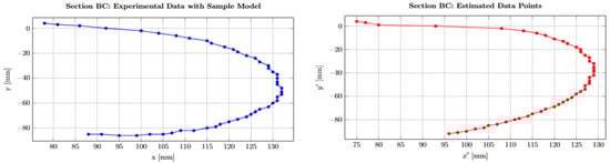
Figure 3. Blade profile regression using parameters $(n,{\gamma }_{n,m}^{\left(N\right)})=(2,1.25)$ with $N=48$ samples.

4.3. Comment on Plot Behavior

Despite the model’s strong overall performance, some localized deviations are apparent, particularly near the blade’s leading edge. As shown in Figure 3, the initial sampled points (notably at $i=1$) exhibit slight divergence from the fitted curve, indicating a localized mismatch in this region. This discrepancy likely arises from higher curvature or structural transitions in the leading edge zone that the current exponential model cannot fully capture without additional parameters.

To investigate this further, Figure 4 plots the Euclidean distances between the actual sample points and their estimated coordinates in Cartesian space. The residuals notably increase starting around $i=40$, coinciding with the profile’s transition into a straighter segment. These systematic deviations indicate that, while the current regression model effectively captures the global shape, refinement is necessary to better represent regions of changing curvature.

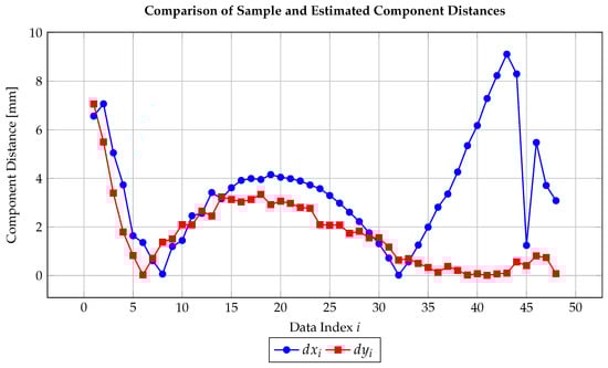
Figure 4. Euclidean distance components $(d{x}_i,d{y}_i)$ between actual sample points and corresponding model estimates in Cartesian coordinates.

Quantitatively, the residual amplitudes observed in Figure 4 remain within $\pm 0.5$ mm for most points, which is consistent with the maximum deviation predicted by the measurement uncertainty ${\sigma }_r=0.29$ mm derived from the preliminary observations. This agreement validates that the fitted regression model reproduces the measured data to within the intrinsic precision of the sampling process.

These findings motivate extending the model by including a third parameter, as discussed in the next subsection. Such enhancement aims to improve local fit accuracy while preserving the model’s overall statistical and geometric integrity.

The localized residual increase near the trailing region (large $\theta$) suggests that the two-parameter exponential model slightly underestimates curvature flattening, as the logarithmic linearisation inherently assumes a constant curvature rate. To account for this non-uniformity, the next section introduces an auxiliary angular component that decouples global curvature scaling (through ${\mathsf{\Theta }}_i$) from local curvature compensation (through ${\Delta }_i$). This refinement preserves the exponential nature of the regression while adding an additional degree of geometric flexibility. Importantly, it directly addresses the measurement-scale residuals previously identified, ensuring that subsequent modelling stages remain consistent with both the experimental resolution and the geometric fidelity of the blade section.

4.4. Three-Parameter Exponential Regression Model in Polar Coordinates

To improve flexibility and capture higher-order curvature effects, the exponential regression model is extended by introducing a third parameter through an auxiliary transformation

$$h:\theta \mapsto \Delta :=h\left(\theta \right),$$

(7)

where $h\in C^{\infty }(D,\mathbb{R})$ is a smooth function independent of the transformation g used for $\mathsf{\Theta }$. The variable ${\Delta }_i$ accounts for additional geometric variations not captured by the two-parameter model.

Accordingly, the model becomes

$$r_i=a{e}^{b{\mathsf{\Theta }}_i+c{\Delta }_i}{e}^{{\epsilon }_i},$$

(8)

where $a>0$, $b,c\in \mathbb{R}$, and ${\epsilon }_i$ represents the residuals. The primary transformation for ${\mathsf{\Theta }}_i$ is retained as

$${\mathsf{\Theta }}_i=g\left({\theta }_i\right){\left({\displaystyle \frac{{\theta }_i+1}{{\theta }_i}}\right)}^{{\displaystyle \frac{1}{2n-1}}},$$

(9)

while the new variable ${\Delta }_i=h\left({\theta }_i\right)$ introduces higher-order angular behaviour. This formulation extends the smooth exponential structure of the previous model, improving arc-length estimation and local curvature representation.

Taking logarithms yields the linearized regression model

$$ln\left(r_i\right)={\beta }_0+{\beta }_1{\mathsf{\Theta }}_i+{\beta }_2{\Delta }_i+{\epsilon }_i,$$

(10)

where ${\beta }_0=ln\left(a\right)$, ${\beta }_1=b$, and ${\beta }_2=c$. The Ordinary Least Squares (OLS) estimation procedure follows directly, with full derivations provided in Supplementary S7. Once the parameters are estimated, the regression model in its original form is reconstructed as

$${\widehat{r}}_i=\widehat{a}{e}^{\widehat{b}{\mathsf{\Theta }}_i+\widehat{c}{\Delta }_i},\mathrm{where}\widehat{a}=e^{{\widehat{\beta }}_0},\widehat{b}={\widehat{\beta }}_1,\widehat{c}={\widehat{\beta }}_2.$$

(11)

To determine an appropriate transformation for ${\Delta }_i$, a monomial mapping is adopted:

$${\Delta }_i={\theta }_i^L,$$

(12)

where $L\in \mathbb{N}$ serves as a tuning parameter controlling higher-order angular contributions. By systematically varying L and analysing the coefficient of determination $R^2$,

$$R^2={\displaystyle \frac{{\sum }_{i=1}^N{(ln{\widehat{r}}_i-\overline{lnr})}^2}{{\sum }_{i=1}^N{(ln{\widehat{r}}_i-\overline{lnr})}^2+{\sum }_{i=1}^N{\widehat{\epsilon }}_i^2}},$$

(13)

the optimal configuration is obtained for $L=1$, corresponding to

$${\widehat{r}}_i=1.78e^{3.95{cos}^{{\displaystyle \frac{3}{2}}}\left({\theta }_i\right){({\theta }_i+1)}^{1/3}-3.61{\theta }_i}\left[\mathrm{mm}\right],$$

(14)

which achieves an excellent fit with $R^2=0.981$. This result highlights the improved capability of the three-parameter model to represent subtle variations in blade curvature and enhance geometric accuracy.

4.5. Graphical Representations

To validate the quality of the regression fit, visual comparisons between the reference sampling points and the estimated profile are presented. Figure 5 illustrates the overlay of the estimated blade profile on the original data points. The two curves align closely across the full angular domain, confirming the model’s effectiveness in capturing the geometry of section $\stackrel{⌢}{\mathrm{BC}}$.

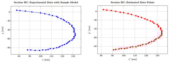
Figure 5. Blade geometry with $L=1$. Estimated profile overlaid on original sampling.

Further support is provided by Figure 6, which plots the Euclidean distance between the Cartesian coordinates of the reference points and the model estimates. The residuals remain consistently small across all points, with no significant outliers or systematic trends. This confirms the stability of the three-parameter regression model and its potential application in quality control or design optimization contexts.

Figure 6. Distance between sample and estimated values for each component (Cartesian coordinates).

In conclusion, the incorporation of a third parameter markedly improves the regression model’s capacity to represent the blade geometry with greater fidelity. By introducing a high-degree polynomial term in the angular coordinate, the model effectively captures both the global curvature and the finer, localized geometric variations of the profile. This refinement enables a more accurate and robust representation of complex blade contours, making the model a valuable analytical tool for predictive design and geometric verification in turbomachinery applications.

5. Analysis of the Reduced Dataset (N = 48)

This section examines the behaviour of the regression model when the dataset is reduced from $N=187$ to $N=48$ sampled points. The reduction aims to test the robustness and geometric fidelity of the model under sparser data conditions while maintaining the essential curvature of the blade section $\stackrel{⌢}{\mathrm{BC}}$. Angular filtering was applied using a ceiling-based selection of points by degree separation, preserving geometric symmetry and avoiding redundant samples. The data, initially in Cartesian coordinates, were converted into polar coordinates $(r,\theta )$ to match the exponential regression formulation adopted throughout this study.

5.1. Regression Model and Statistical Evaluation

The nonlinear regression model describing the radius as a function of the angular coordinate is given by Equation (14) where the exponential terms capture the smooth curvature of the blade in polar coordinates. The parameters were obtained via least squares fitting applied to the reduced sample of $N=48$ points.

The model achieves a coefficient of determination of $R^2=0.981$, indicating that 98.1% of the observed variance is explained by the regression, and a residual variance of $\mathrm{Var}\left(\widehat{\epsilon }{\widehat{\epsilon }}^T\right)=0.047113$, confirming low dispersion of residuals. Figure 5 and Figure 6 illustrate, respectively, the fitted profile and the pointwise deviations between measured and estimated coordinates. The results demonstrate that the regression captures the essential geometric features of the blade even with significantly fewer sampling points.

5.2. Sensitivity to the Angular Parameter

The influence of the angular exponent parameter m on the model’s performance is analysed in Figure 7, where $R^2$ is plotted as a function of m. The curve reveals a distinct optimum where $R^2$ reaches its maximum, indicating that appropriate tuning of m enhances the fit without overfitting. This sensitivity analysis confirms that the proposed transformation terms provide both flexibility and stability across varying sampling densities.

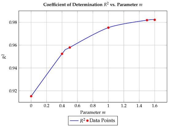
Figure 7. Coefficient of determination across different values of m.

5.3. Model Robustness and Observations

Overall, the regression demonstrates strong predictive accuracy and structural stability. Only a few points (approximately five of 48) show noticeable deviations, likely due to local irregularities or measurement noise. Both the leading and trailing edges of the profile match the reference geometry closely, ensuring the continuity of the blade contour, a crucial requirement for aerodynamic and manufacturing integrity.

Despite discretisation introduced by practical tools (e.g., ceiling rounding in measured $r_i$), the model remains consistent with the theoretical assumptions of Ordinary Least Squares: linearity in parameters, homoscedasticity, and independent residuals. This confirms that the regression procedure is both statistically sound and geometrically reliable for practical use in turbine blade validation and control (Supplementary S4, S5 and S7).

6. Arc Length of Section $\stackrel{⌢}{\mathrm{BC}}$

This section focuses on the computation of the arc length corresponding to section $\stackrel{⌢}{\mathrm{BC}}$ of the turbine blade profile. The arc length is a key geometric metric for validating the regression formulation and ensuring that the reconstructed profile preserves geometric and physical fidelity. The calculation employs the parametric form of the regression models in polar coordinates, evaluated numerically through Gauss–Legendre quadrature methods commonly used in computational geometry and mechanics [12,17,18].

6.1. Arc Length in Polar Coordinates

For a smooth curve $r=r\left(\theta \right)$, the arc length between angular limits ${\theta }_1$ and ${\theta }_2$ is defined as

$$I={\int }_D\sqrt{r^2+{\left({\displaystyle \frac{dr}{d\theta }}\right)}^2}d\theta ,$$

(15)

where $D=\left[\frac{-44\pi }{180},\frac{3\pi }{180}\right]$ represents the angular domain for the section under study. The function $r\left(\theta \right)$ corresponds to the estimated radius from the nonlinear regression model in Equation (14). This classical formulation captures both radial and tangential variations of the curve, allowing numerical evaluation of the blade’s total geometric length (Supplementary S2, S3, S6, S8 and S9).

6.2. Generalized Three-Parameter Arc Length Model

Extending the analysis to the three-parameter regression model,

$$\begin{array}{c}\hfill \widehat{r}\left(\theta \right)={\widehat{a}}_{n,m}^{(N,L)}exp\left[{\widehat{b}}_{n,m}^{(N,L)}{(\theta +1)}^{{\displaystyle \frac{1}{2n-1}}}{cos}^{{\gamma }_{n,m}^{(N,L)}}\left(\theta \right)+{\widehat{c}}_{n,m}^{(N,L)}{\theta }^L\right],\end{array}$$

(16)

the generalized arc length expression becomes

$$I_{n,m}^{(N,L)}={\int }_D\left|{\widehat{a}}_{n,m}^{(N,L)}\right|e^{{\widehat{b}}_{n,m}^{(N,L)}{(\theta +1)}^{{\displaystyle \frac{1}{2n-1}}}{cos}^{{\gamma }_{n,m}^{(N,L)}}\left(\theta \right)+{\widehat{c}}_{n,m}^{(N,L)}{\theta }^L}{F}_{n,m}^{(N,L)}\left(\theta \right)d\theta ,$$

(17)

where the derivative term $F_{n,m}^{(N,L)}\left(\theta \right)$ represents the radial-rate contribution within the integrand. Its explicit analytical form and proof of integrability are detailed in Supplementary S8. Since the integrand remains continuous and differentiable across D, Equation (17) can be stably evaluated using Gauss–Legendre quadrature.

6.3. Numerical Evaluation and Comparison

Arc length calculations were performed for both the two- and three-parameter regression models using $N=48$ and $N=187$ sampled points across the domain D = [−0.76794, 0.05362].

• Case 1: Two-parameter model.

Using Equation (6) with $n=m=2$, the two-parameter model yields an interpolated arc length of approximately $145\mathrm{mm}$ according to CATIA. However, a singularity at $\theta =0$ prevents differentiation and direct numerical integration, limiting the precision of standard quadrature approaches.

• Case 2: Three-parameter model.

Introducing a third parameter resolves this limitation, producing the refined model in Equation (14), which yields an arc length of about $149\mathrm{mm}$.

This result differs by less than $3\%$ from CATIA’s spline-based estimation ($146.77\mathrm{mm}$) and by approximately $4\%$ from the analytical reference value ($142.83\mathrm{mm}$) (Figure 8). A numerically stable alternative model,

$${\widehat{r}}_i=0.5267e^{5.19{cos}^{{\displaystyle \frac{1}{2}}}\left({\theta }_i\right){({\theta }_i+1)}^{1/3}-3.537{\theta }_i}\left[\mathrm{mm}\right],$$

(18)

achieves a coefficient of determination of $R^2=0.958$ and yields consistent arc-length estimates in the range of 144–$145\mathrm{mm}$ under Gauss–Legendre quadrature with 2–5 points. These results are also in agreement with both the computed estimative value of $145.54\mathrm{mm}$ and CATIA’s spline-derived result of $146.77\mathrm{mm}$, confirming the enhanced numerical robustness and reliability of the proposed formulation for integration-based applications. (Figure 9).

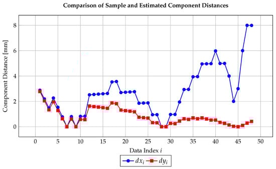
Figure 8. Component distances $d{x}_i$ and $d{y}_i$ as functions of data index i.

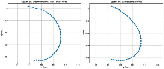
Figure 9. Blade geometry for parameter configuration $(n,m,L)=(2,0.5,1)$. The estimated profile is superimposed on the original sampled points, incorporating arc length correction to enhance geometric accuracy.

Despite small structured residuals near the leading edge, the global curvature and length agreement remain strong. These results demonstrate that the exponential regression formulation reproduces the reference blade geometry within less than $4\%$ deviation from CATIA-derived spline values, confirming its reliability for analytical validation and manufacturing quality assessment.

The comparative analysis between the two- and three-parameter formulations reveals the decisive role of the functional structure in determining geometric accuracy. While the two-parameter model already provides a reliable global fit, the inclusion of an additional nonlinear term enhances local adaptability, particularly in regions with rapid curvature variation. This flexibility is essential for achieving accurate predictions in turbine blade manufacturing and quality assessment.

Nevertheless, the three-parameter formulation also exposes certain challenges inherent to regression-based geometric modelling. The separation of the last four data points in Figure 10 indicates localized deviations near the blade edges, where curvature changes abruptly. If only the smoother central region were evaluated, the $R^2$ value could be artificially inflated, leading to a misleading interpretation of model performance. This observation underscores the importance of evaluating the entire dataset, ensuring that both global and local accuracy criteria are satisfied. Overall, the three-parameter formulation attains an optimal balance between smoothness, flexibility, and numerical stability, making it particularly suitable for high-precision engineering validation.

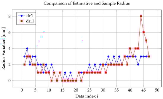
Figure 10. Comparison of dr’l and dr_l values.

The regression parameters reported in Table 1 and Table 2 underscore the advantages of the three-parameter model for arc-length reconstruction in Section BC. While the two-parameter formulation captures the global trend, its singular behaviour near $\theta =0$ limits numerical integration. The three-parameter model provides greater flexibility, improved stability, and higher accuracy, yielding arc-length values consistent with CATIA and analytical references. Overall, the additional parameter enables better representation of localized curvature variations and more reliable geometric evaluation.

Table 1. Two-parameter regression results for $N=48$.

Parameter	Value
${\widehat{\beta }}_0$	93.27147829
${\widehat{\beta }}_1$	−0.583051778
R	−0.967985577

Table 2. Three-parameter regression results for $N=48$.

Parameter	Value
${\widehat{\beta }}_0$	0.5267
${\widehat{\beta }}_1$	5.19
${\widehat{\beta }}_2$	−3.537
$R^2$	0.958

7. Conclusions

By substituting the regression model (18) into the arc-length formulation (17), the computed arc length of section $\stackrel{⌢}{\mathrm{BC}}$ was approximately $145\mathrm{mm}$, closely matching the reference measurement of $146.778\mathrm{mm}$ and achieving a precision of 98.79%. This result was obtained using a five-point Gauss–Legendre quadrature, ensuring both numerical accuracy and computational efficiency.

The reliability of the proposed methodology stems from the precision of the input data and the statistical robustness of the OLS estimation process. Even when data reduction techniques, such as the ceiling function, are applied to the radius, the model preserves the essential OLS properties and minimizes the Euclidean distance between observed and predicted Cartesian coordinates. the formulation preserves over 98% geometric fidelity in arc-length estimation, even when the dataset is significantly reduced.

The three-parameter formulation proves particularly effective in regions with strong curvature gradients, capturing local geometric variations that simpler models cannot. Future extensions should explore analytical expressions for the arc-length integrals, evaluate higher-order quadrature schemes, and refine residual control near the blade edges. Future work should consider treating the last four data points as localised edge cases to further improve predictive stability.

In summary, the proposed regression formulation constitutes a precise, compact, and reproducible analytical tool for geometric verification in cross-flow turbine blades. Its integration into quality control and manufacturing workflows can improve both design reliability and production efficiency, bridging the gap between mathematical modeling and practical engineering implementation.

References

- Moya, G.A. Modelación de Parámetros Geométricos Para un Álabe Direccional de una Turbina de Media Potencia; Universidad de La Frontera: Temuco, Chile, 2015. [Google Scholar]
- Scheurer, H.; Matzler, R.; Yoder, B. Small Water Turbine: Instruction Manual for the Construction of a Cross Flow Turbine; German Appropriate Technology Exchange (GATE); Deutsches Zentrum für Entwicklungstechnologien: Eschborn, Germany, 1980. [Google Scholar]
- Breslin, W.R. Small Michell-Banki Turbine: A Construction Manual; Volunteers in Technical Assistance: Mt. Rainier, MD, USA, 1979. [Google Scholar]
- Dassault Systèmes. CATIA V5 User Guide: Mechanical Design Workbenches; Dassault Systèmes: Cedar City, UT, USA, 2013. [Google Scholar]
- Seber, G.A.F.; Lee, A.J. Linear Regression Analysis, 2nd ed.; Wiley: Hoboken, NJ, USA, 2003. [Google Scholar]
- Wooldridge, J.M. Introductory Econometrics: A Modern Approach, 7th ed.; Cengage Learning: Boston, MA, USA, 2019. [Google Scholar]
- Greene, W.H. Econometric Analysis, 7th ed.; Pearson Education: London, UK, 2012. [Google Scholar]
- Montgomery, D.C.; Peck, E.A.; Vining, G.G. Introduction to Linear Regression Analysis, 5th ed.; Wiley: Hoboken, NJ, USA, 2012. [Google Scholar]
- Figaschewsky, F.; Kühhorn, A.; Giersch, T. A higher order linear least square fit for the assessment of integral and Non-Integral vibrations with blade tip timing. In Proceedings of the 17th International Symposium on Transport Phenomena and Dynamics of Rotating Machinery (ISROMAC2017), Maui, HI, USA, 16–21 December 2017. [Google Scholar]
- Laurie, D. Calculation of Gauss-Kronrod quadrature rules. Math. Comput. 1997, 66, 1133–1145. [Google Scholar] [CrossRef]
- Hunt, A.; Strom, B.; Talpey, G.; Ross, H.; Scherl, I.; Brunton, S.; Wosnik, M.; Polagye, B. An experimental evaluation of the interplay between geometry and scale on cross-flow turbine performance. Renew. Sustain. Energy Rev. 2024, 206, 114848. [Google Scholar] [CrossRef]
- Press, W.H.; Teukolsky, S.A.; Vetterling, W.T.; Flannery, B.P. Numerical Recipes: The Art of Scientific Computing, 3rd ed.; Cambridge University Press: Cambridge, UK, 2007. [Google Scholar]
- Kariman, H.; Hoseinzadeh, S.; Khiadani, M.; Nazarieh, M. 3D-CFD analysing of tidal Hunter turbine to enhance the power coefficient by changing the stroke angle of blades and incorporation of winglets. Ocean Eng. 2023, 287, 115713. [Google Scholar] [CrossRef]
- González-Barrio, H.; Calleja-Ochoa, A.; Lamikiz, A.; López; de Lacalle, L.N. Manufacturing processes of integral blade rotors for turbomachinery, processes and new approaches. Appl. Sci. 2020, 10, 3063. [Google Scholar] [CrossRef]
- Mosonyi, E. Water Power Development: Volume 1—Low Head Power Plants; Akadémiai Kiadó: Budapest, Hungary, 1963. [Google Scholar]
- Paish, O. Small Hydro Power: Technology and Current Status. Renew. Sustain. Energy Rev. 2002, 6, 537–556. [Google Scholar] [CrossRef]
- Farin, G. Curves and Surfaces for CAGD: A Practical Guide, 5th ed.; Morgan Kaufmann: Burlington, MA, USA, 2002. [Google Scholar]
- Burden, R.L.; Faires, J.D.; Burden, A.M. Numerical Analysis, 10th ed.; Cengage Learning: Boston, MA, USA, 2016. [Google Scholar]
Disclaimer/Publisher’s Note: The statements, opinions and data contained in all publications are solely those of the individual author(s) and contributor(s) and not of MDPI and/or the editor(s). MDPI and/or the editor(s) disclaim responsibility for any injury to people or property resulting from any ideas, methods, instructions or products referred to in the content. |
© 2025 by the authors. Licensee MDPI, Basel, Switzerland. This article is an open access article distributed under the terms and conditions of the Creative Commons Attribution (CC BY) license (https://creativecommons.org/licenses/by/4.0/).