Article

Cross-Embodiment Kinematic Behavioral Cloning (X-EKBC): An Energy-Based Framework for Human–Robot Imitation Learning with the Embodiment Gap

Department of Mechatronics Engineering, Graduate School of Science and Technology, Meijo University, 501-1 Shiogamaguchi, Nagoya 468-8502, Japan
*
Author to whom correspondence should be addressed.
These authors contributed equally to this work.
Machines 2025, 13(12), 1134; https://doi.org/10.3390/machines13121134
Submission received: 11 November 2025 / Revised: 2 December 2025 / Accepted: 8 December 2025 / Published: 10 December 2025
(This article belongs to the Special Issue Robots with Intelligence: Developments and Applications)

Abstract

In imitation learning with the embodiment gap, directly transferring human motions to robots is challenging due to differences in body structures. Therefore, it is necessary to reconstruct human motions in accordance with each robot’s embodiment. Our previous work focused on the right arm of a humanoid robot, which limited the generality of the approach. To address this, we propose Cross-Embodiment Kinematic Behavioral Cloning (X-EKBC), an imitation learning framework that enables movement-level imitation on a one-to-one basis between humans and multiple robots with embodiment gaps. We introduce a joint matrix that represents the structural correspondence between the human and robot bodies, and by solving kinematics based on this matrix, the system can efficiently reconstruct motions adapted to each robot’s embodiment. Furthermore, by employing Implicit Behavioral Cloning (IBC), the proposed method achieves both imitation learning of the reconstructed motions and quantitative evaluation of embodiment gaps using energy-based modeling. As a result, motion reconstruction through the joint matrix became feasible, enabling both imitation learning and quantitative embodiment evaluation based on reconstructed behaviors. Future work will aim to extend this framework toward motion-level imitation that captures higher-level behavioral outcomes.

1. Introduction

Driven by population aging and labor shortages, interest in robotic automation has grown steadily as industries seek sustainable solutions to workforce constraints. Among these technologies, imitation learning has attracted significant attention because it enables robots to acquire skills through intuitive demonstrations rather than requiring specialized programming. Imitation learning is a framework in which an agent learns to reproduce a demonstrated behavior by observing a teacher.
However, imitation learning remains challenging since the morphological and kinematic discrepancies between humans and robots create an embodiment gap [1]. Embodiment refers to the physical and functional characteristics specific to a robot, such as joint structure, link length, sensor configuration, actuation method, and control specifications. As shown in Figure 1, the embodiment gaps make it difficult to directly map human motions onto robots.
Embodiment can be broadly categorized into two types: a priori embodiment and a posteriori embodiment. A priori embodiment includes static and predictable elements such as kinematic structure, joint configuration, sensor arrangement, and control specifications. In contrast, a posteriori embodiment encompasses dynamic aspects such as robot dynamics, actuator and sensor response characteristics, and control performance, which can only be recognized through motion execution and interaction with the environment. This research focuses specifically on embodiment gaps arising from kinematic structures such as link configuration and joint arrangement.
If human and robot kinematic structures were identical, direct imitation would be possible. However, differences in joint ranges of motion and degrees of freedom often lead to undefined or non-corresponding joint angles. As a result, it becomes difficult to uniquely determine corresponding joint angles, which may cause trajectory discontinuities or physically infeasible postures. Therefore, for effective imitation, a robot must infer human intentions from observed motion and re-synthesize these actions in forms feasible within its own kinematic constraints.
Imitation can be broadly classified into three levels:
  • Motion-level imitation: imitation involves directly mapping the demonstrator’s limb trajectories onto the robot’s corresponding joints, reproducing the observed kinematics.
  • Result-level imitation: Reproducing the results of actions such as picking and placing objects.
  • Intent-level imitation: Imitation that incorporates intent. For example, whether the action is intended for pick-and-place or merely to move something out of the way.
Previous studies have addressed this issue in two phases: during demonstration data collection and during learning. During data collection, direct teaching methods have been widely adopted to bypass embodiment gaps. Examples include teleoperation [2] and kinesthetic teaching [3], where human operators directly manipulate the robot. These approaches inherently account for the robot’s kinematics, but they require access to physical hardware and involve high setup and operational costs. During learning, policy learning approaches have been explored to absorb embodiment gaps. Methods based on deep reinforcement learning [4] and inverse reinforcement learning [5] enable robots to acquire structure-adaptive policies through trial and error. Other attempts leverage Energy-Based Models (EBMs) [6] and Implicit Behavioral Cloning (IBC) [7] to directly model action distributions tailored to different embodiments [8].
Our previous work [8] evaluated embodiment gaps by considering the trade-off between joint angles and end-effector pose. However, the approach was limited to the right arm of a humanoid robot and was not extended to multiple robots with different structures. To enable imitation across diverse robots, a framework is required that can formally and consistently represent different kinematic structures. Furthermore, quantitative evaluation of embodiment gaps in motion-level imitation learning remains an open challenge.
This study proposes the Cross-Embodiment Kinematic Behavioral Cloning (X-EKBC) imitation learning framework, enabling one-to-one action-level imitation between humans with embodied differences and multiple robots. To achieve this, we mathematically express kinematic structures and introduce joint matrices [9] that explicitly evaluate embodied differences arising from link and joint configurations. Furthermore, using IBC based on an EBM, we achieve action-level imitation learning beyond embodiment and quantitatively evaluate differences in embodiment due to energy for the first time.
In addition to these theoretical contributions, our framework brings practical advantages to robot system design. The ability to reuse the same human demonstration data across multiple robot platforms reduces development costs and manual teaching efforts. In addition, the quantitative evaluation of embodiment gaps enables us to determine which robot platform is more suitable for the imitation of specific human motions. This provides a principled basis for selecting or designing robot embodiments that are better aligned with human motor behavior.
Unlike direct teaching approaches [3,4], the proposed method operates within the framework of Imitation from Observation (IfO), requiring only observational data. Our scope is restricted to motion-level imitation, leaving result-/intent-level generalization to future work.
The contributions of this research are summarized as follows:
  • Generalization of robot kinematics using the joint matrix, enabling consistent imitation learning across robots with different structures using the same human demonstration data.
  • Energy-based evaluation of embodiment gaps, allowing quantitative assessment of embodiment gaps and enabling motion-level comparison across robots with heterogeneous structures, which has been difficult in conventional approaches.
The structure of this paper is as follows. Section 1 introduces the research background and objectives. Section 2 reviews related work. Section 3 presents the proposed X-EKBC framework, which integrates the novel concept of a joint matrix for preprocessing demonstration motions with an Energy-Based Model for learning embodiment-invariant representations and estimating imitation behaviors. Section 4 reports the experimental results of the proposed system, first validating the motion transformation process and then evaluating the outcomes of imitation learning. Finally, Section 5 concludes the paper with a summary of the findings.

2. Related Work

2.1. Demonstration Collection Methods Addressing Embodiment Gaps

To create teaching data for robots, direct teaching and teleoperation have been widely used. In direct teaching, a human physically manipulates the robot’s links or arms to record the motion data [3]. Teleoperation enables data collection through Virtual Reality (VR) or Mixed Reality (MR) interfaces [4,10].
To unify observation and action spaces between humans and robots, various shared interfaces have been proposed. LEGATO [11] employs a handheld gripper with an integrated camera, enabling policy learning in tool space and subsequent zero-shot transfer to robots via inverse kinematics. MIME [12] collected large paired datasets of human demonstration videos and robot kinesthetic demonstrations, enabling direct mapping from vision to actions. Motion retargeting has also been widely adopted. For example, Yang et al. [13] generated optimized trajectories from a small number of VR demonstrations, constructing datasets applicable to different robotic arms. ODIL [14] synchronized bimanual coordination through visual servoing, reproducing multiple bimanual tasks from a single demonstration.
Another effective approach is object-centric representation. Methods such as Human2Sim2Robot [15] and X-Sim [16] extract object trajectories from demonstration videos and use them as task goals, enabling imitation across different embodiments.
Although direct teaching reduces the impact of structural differences, it requires operator expertise and individual demonstrations for each robot, making large-scale deployment costly. Therefore, imitation learning from observation alone offers a promising alternative to reduce this cost.

2.2. Imitation Learning Approaches

2.2.1. Behavioral Cloning as a Baseline

A fundamental baseline for imitation learning is Behavioral Cloning (BC) [17], where a neural network is trained to map observed states to demonstrated actions. By inference, the learned state–action model enables imitation. However, BC suffers from two major issues: distribution shift and action averaging.
Distribution shift occurs when the robot encounters states outside the training distribution, leading to unstable behavior. To mitigate this, Guided Cost Learning (GCL) [18] estimates a cost function from demonstrations and imitates behavior by following it, while Generative Adversarial Imitation Learning (GAIL) [19] employs a generator–discriminator setup with reinforcement learning to achieve robustness to unseen states. Cross-embodiment Inverse Reinforcement Learning (XIRL) [5] leverages inverse reinforcement learning to infer a reward function from demonstrations, enabling policies resilient to distribution shift.
Action averaging arises when multiple valid behaviors are averaged into suboptimal motions. Action Chunking with Transformers (ACT) [20] avoids this by leveraging sequence modeling. In GAIL, the discriminator forces the generator to produce diverse behaviors, mitigating averaging.
To address both issues, Implicit Behavioral Cloning (IBC) [7] employs an Energy-Based Model (EBM) for contrastive learning, treating demonstration actions as positive examples and others as negatives. This formulation avoids distribution shift and captures multi-modality by representing multiple valid actions as distinct low-energy solutions.

2.2.2. Addressing Embodiment Gap

A central challenge in imitation learning is that the demonstrator and the robot often have different embodiments. Methods based on feature space alignment and domain adaptation have been proposed to overcome embodiment gaps. XIRL [5] uses self-supervised learning to obtain embodiment-invariant embeddings of task progress, which are then used as rewards in reinforcement learning. Learn What Matters [21] employs mutual information constraints and adversarial training to extract only task-relevant features. GWIL [22] applies optimal transport to align state spaces across embodiments. Time-Contrastive Networks [23] learn a mapping between human and robot joint configurations by training on paired videos, enabling motion imitation.
Skill abstraction is another promising approach. XSkill [24] and UniSkill [25] decompose videos of human and robot demonstrations into short segments, learning skill prototypes. Tasks are then represented as sequences of skills, enabling zero-shot execution of novel tasks. UniSkill, in particular, leverages large-scale cross-embodiment video data to improve generalization. O2A (One-Shot Observational Learning with Action Vectors) [26] extracts action vectors from third-person human demonstrations and compares them with robot execution vectors to design rewards for reinforcement learning, enabling imitation from a single demonstration.
In reinforcement learning-based approaches, Taylor et al. [4] applied Proximal Policy Optimization with a reward function designed to favor human-like actions, enabling robots to learn human-like motions. There are also examples of overcoming embodiment gaps through large-scale data aggregation. The X-Embodiment project [27] collected demonstrations on 22 robot platforms and trained a single Transformer-based policy across embodiments. However, the scalability of this approach is limited as the Transformer model grows with the number of robots.
Despite these advances, embodiment gaps at the motion level remain difficult to evaluate. End-effector trajectories and joint angles often present a trade-off, making it challenging to assess overall motion similarity. Existing works primarily evaluate imitation by task success rates or generalization performance, but they lack a framework for quantitatively measuring embodiment gaps.

2.2.3. Imitation from Observation

Another line of research explores Imitation from Observation (IfO), where robots learn from videos or other sensory data without access to demonstrator actions. Humans naturally learn this way by observing others, inferring appropriate actions based on their own embodiment. Torabi et al. [28] proposed an approach where an agent first learns a BC policy to infer actions from state transitions, then retrains it by comparing its own observations with those of a human demonstration. Replacing the BC model with a GAIL-based policy enabled comparable performance in high-dimensional action spaces [29]. Further, by mapping visual inputs to joint angles, learning speed was improved. RIDM (Reinforced Inverse Dynamics Modeling) [30] acquires a policy by reinforcement learning to predict actions from state transitions, enabling imitation from a single demonstration. DEALIO (Data-Efficient Adversarial Learning for IfO) [31] replaces the GAIL generator with a linear-quadratic regulator controller, improving sample efficiency.
Other works focus on embodiment adaptation in IfO. Hudson et al. [32] showed that when only link lengths differ between humans and robots, an affine transformation function can be learned such that transformed skeletons fool the GAIL discriminator, thus adapting to length differences. Hiruma et al. [33] proposed a deep active visual attention framework in which the robot learns to autonomously focus on task-relevant regions, enabling selective imitation and tool-body assimilation during motion generation.
In our previous work [8], we investigated imitation across humanoid robots with different joint and link structures. Embodiment gaps were estimated using the Levenberg-Marquardt method [34], enabling the separation of motion into end-effector-centric and joint-angle–centric components. These were then learned through Energy-Based Models within the framework of Implicit Behavioral Cloning.
However, our previous researches [8] have focused solely on the right arm of humanoid robots, without addressing applicability to a broader range of robots. To overcome this limitation, it is necessary to generalize the method so that it can account for differences in joint structures between the demonstrator and the target robot.

3. Cross-Embodiment Kinematic Behavioral Cloning (X-EKBC)

3.1. System Architecture of X-EKBC

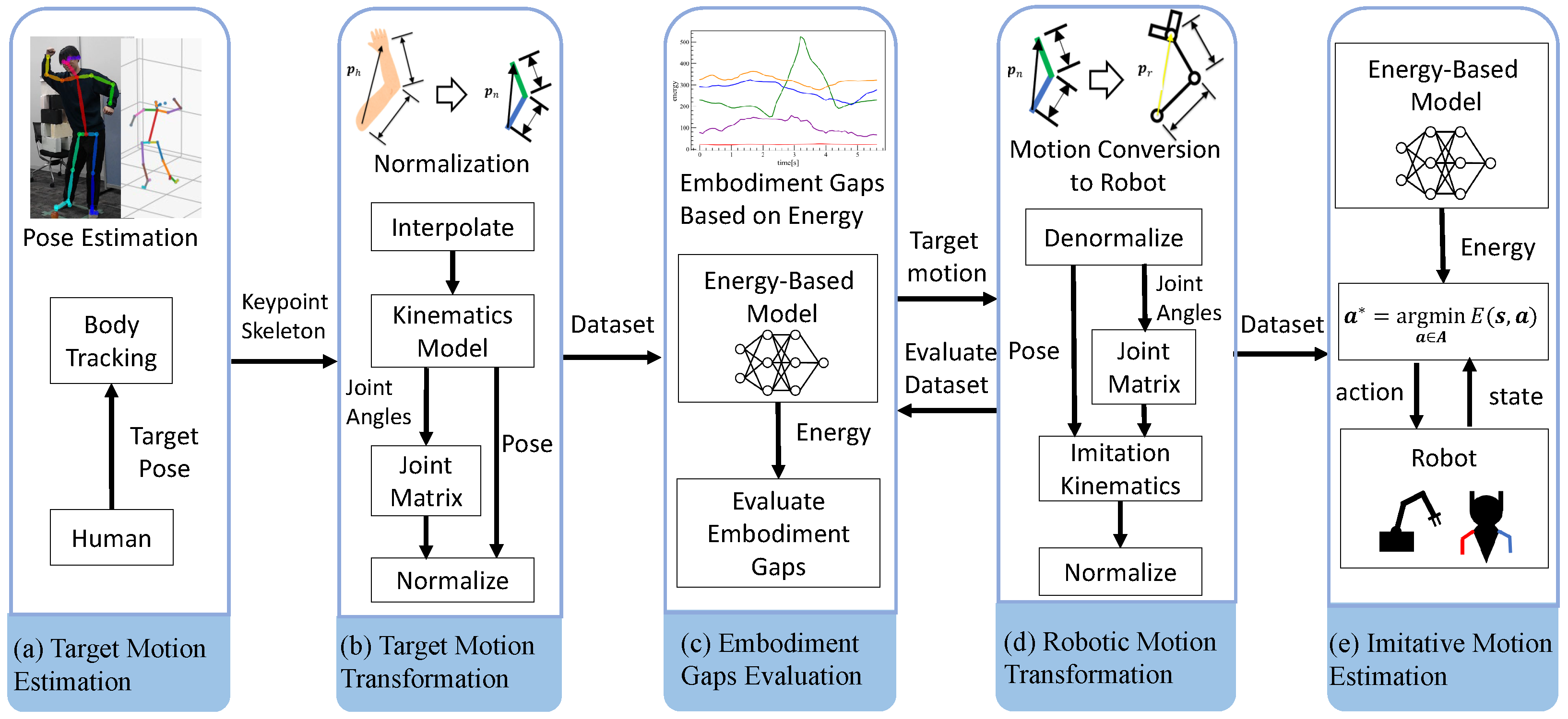
In this study, we propose the X-EKBC System, which enables a robot to imitate human motions based on an evaluation of embodiment gaps between the demonstrator and the robot. The overall system architecture of X-EKBC is illustrated in Figure 2. The input to X-EKBC is the visual observation of the demonstrator, and the output is the robot’s imitation policy. Therefore, X-EKBC belongs to the framework of Imitation from Observation (IfO), since imitation learning can be conducted simply by observing the demonstrator.
The X-EKBC system is organized into five phases.
  • In Figure 2a, the demonstrator’s motion is estimated. This is achieved by extracting a skeletal model from visual recordings of the demonstrator.
  • In Figure 2b, the estimated motion undergoes preprocessing for generalization. Specifically, joint angles and end-effector poses are computed from the skeletal model, followed by normalization of feasible motion ranges and transformation into a matrix form using the newly defined joint matrix.
  • In Figure 2c, an embodiment model of the demonstrator is learned. This model is represented in the form of an EBM.
  • In Figure 2d, the embodiment gaps between the demonstrator and the robot are evaluated. The demonstrator’s motion is transformed into multiple candidate trajectories adapted to the robot’s embodiment, and the learned embodiment model is used to select the transformation that minimizes embodiment discrepancy.
  • Finally, in Figure 2e, the robot learns an imitation behavior model, which is also trained using an EBM.

3.2. Acquisition of Demonstrator Motion Through Observation

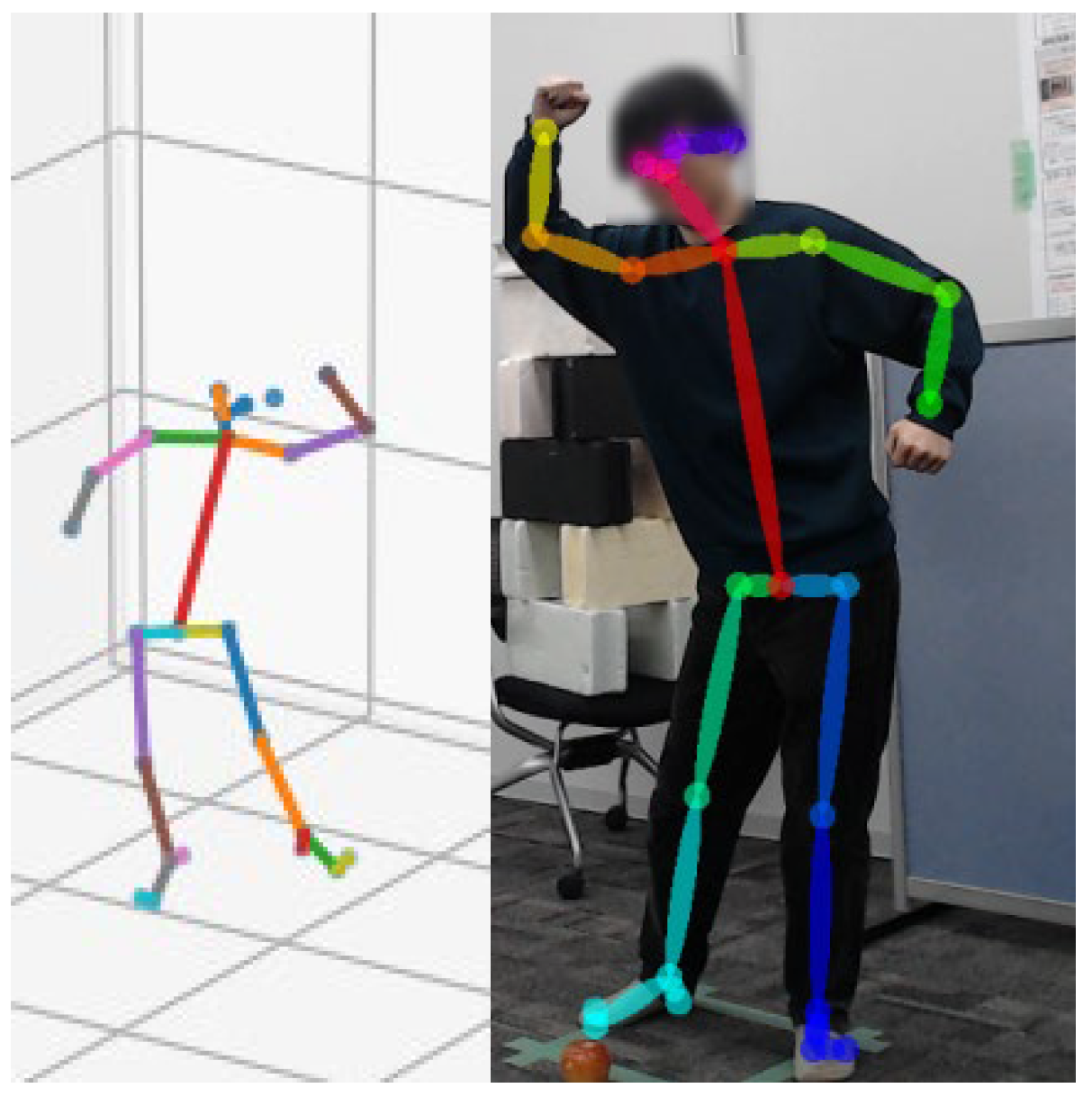
Human joint positions are represented as a keypoint skeleton, in which joints are connected by straight lines. The skeleton format adopted here is the OpenPose BODY25 [35], a standard representation consisting of 25 keypoints estimated by OpenPose. OpenPose performs bottom-up pose estimation by first detecting 2D joint heatmaps and part affinity fields (PAFs) from RGB images using a convolutional neural network. The detected keypoints are then grouped into individual skeletons based on the PAF connections, allowing robust estimation of human posture even in multi-person or partially occluded scenes. When multiple cameras are available, 3D coordinates of each keypoint can be reconstructed by triangulating the corresponding 2D detections from different viewpoints. Figure 3 shows an example of human pose estimation obtained using OpenPose.
For motion capture, we employ both OpenPose and the Azure Kinect sensor. In the case of OpenPose, multiple cameras and sufficient space for camera placement are required to estimate three-dimensional joint coordinates. By contrast, Azure Kinect can estimate 3D joint positions using a single device, making it applicable in a wider range of environments. Azure Kinect leverages not only RGB images but also depth information to estimate human joint coordinates. Moreover, since Azure Kinect provides both joint positions and surrounding object positions within the same coordinate system, it offers an advantage for integrated perception. The skeleton estimated by Azure Kinect consists of 32 joints. Therefore, we convert it into the OpenPose BODY25 format for consistency in this study.
This study assumes that human pose estimation is sufficiently accurate for the target tasks, and errors caused by occlusion, fast motion, complex backgrounds, or sensing limitations are not explicitly considered.

3.3. Motion Transformation of the Demonstrator

3.3.1. Normalization of the Motion Space

To address the scale differences between the demonstrator and the robot, the demonstrator’s motion is normalized to compensate for scale differences. Humans and robots differ in overall body size, resulting in different feasible motion spaces. Therefore, it is necessary to unify the motion space. For this purpose, the lengths of the body segments of both the demonstrator and the robot must first be obtained. When the demonstrator is a human, segment lengths can be extracted from the estimated human keypoint skeleton. For the robot, the lengths of each link can be obtained from the information described in its URDF file. The scale constant is then defined as
d = i N l i n k l i
where d represents the scaling factor. N l i n k represents the number of links in the moving body part, and l i denotes the length of each link.
Let the scale constant of the human body segment be denoted as d h , and that of the robot as d r . The human end-effector position and joint angles calculated from the keypoint skeleton are denoted as p h and q h , respectively. Similarly, the robot’s end-effector position and joint angles are also denoted as p r and q r . Using the scale constant d obtained from Equation (1), these quantities are transformed into the robot’s motion space as follows:
p r = d r d h p h .

3.3.2. Transformation of Joint Configurations

To address differences in joint configurations between demonstrators and robots, we propose a joint matrix that formally represents joint structures. First, in the joint configuration, we group closely connected joints into joint units. Each joint unit contains no joint angles with elements on the same rotational axis. For example, for a 7-degree-of-freedom human: 3 degrees of freedom at the shoulder joint, 2 at the elbow joint, and 2 at the wrist joint. Given the number of joint units N j o i n t , the joint matrix K is defined as follows:
K = [ k 1 k 2 k N j o i n t ] T , k i R 3 , k i j = { 0 , 1 , 2 , 3 } .
The rules for constructing the joint matrix are as follows:
  • Neighboring joints that are physically connected are grouped and treated as a single joint unit.
  • Each joint unit contains only one element for each rotational axis.
  • The elements within a joint unit are numbered according to the order of the rotational axes, counting from the base link.
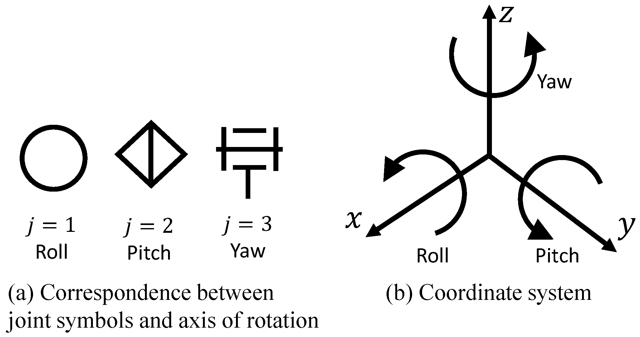
Figure 4 illustrates the coordinate system used to define the joint matrix, as well as the correspondence between the joint notation and the mechanical structure. In the joint matrix, the columns represent each joint unit, while the rows correspond to the three rotational axes: roll, pitch, and yaw, arranged from left to right. The elements of each row indicate the order of joints within a joint unit, starting from the base link. A value of 0 denotes that no joint angle exists for the corresponding rotational axis. For clarity, the definitions of these notations are summarized in Table 1.
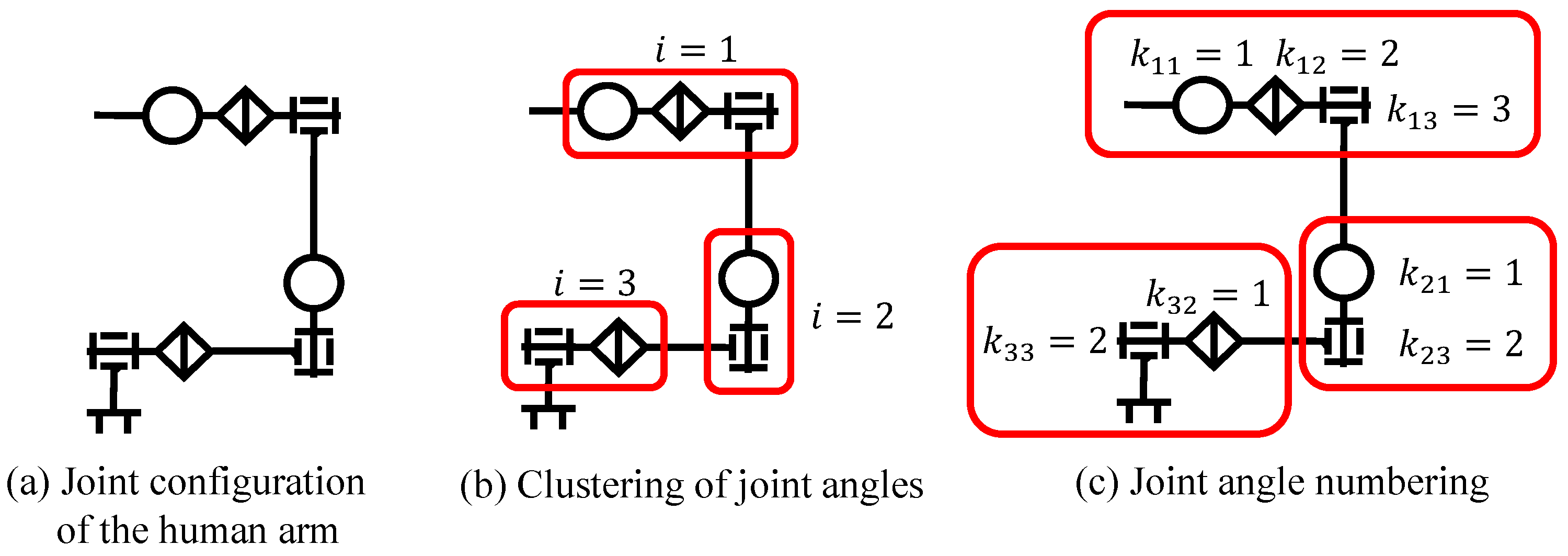
For example, let us first describe the joint matrix of the human arm. A model of the human arm is shown in Figure 5a. As shown in Figure 5b, the joints of the human arm can be grouped into three joint units. Within each joint unit, the joint angles are numbered sequentially starting from the base link, yielding the elements k i j as shown in Figure 5c. The undefined k i j elements corresponding to non-existent joint angles are filled with zeros, and the joint matrix K h u m a n for the human arm is defined as follows:
K h u m a n = 1 2 3 1 0 2 0 1 2 .
Next, we describe the joint angle matrix using the example of a human arm. Since a human arm has seven joint angles, the joint angle vector q h u m a n is defined as follows:
q h u m a n = [ θ 1 h θ 2 h θ 3 h θ 4 h θ 5 h θ 6 h θ 7 h ] T .
Here, θ 1 denotes the joint angle closest to the base link, while θ 7 corresponds to the joint angle closest to the end link. Based on Equations (4) and (5), the joint angle vector q h u m a n is transformed into the joint angle matrix Q h u m a n using K h u m a n as follows:
Q h u m a n = θ 1 h θ 2 h θ 3 h θ 4 h 0 θ 5 h 0 θ 6 h θ 7 h .
Using the joint angle matrix (JAM), the demonstrator’s joint configuration can be systematically mapped to that of the robot. When the numbers of joint units are equal, the Joint Angle Matrices of the demonstrator, q target , and the robot, Q r o b o t , have the same dimensions, allowing direct conversion between them. However, Q r o b o t and q target are not necessarily identical. This is because, in constructing the joint angle matrix, any joints that exist only in the demonstrator are treated as inactive and their corresponding angles are set to zero in Q r o b o t .
As an example, we describe the conversion of human joint angles into those of a robot that has the same number of joint units.
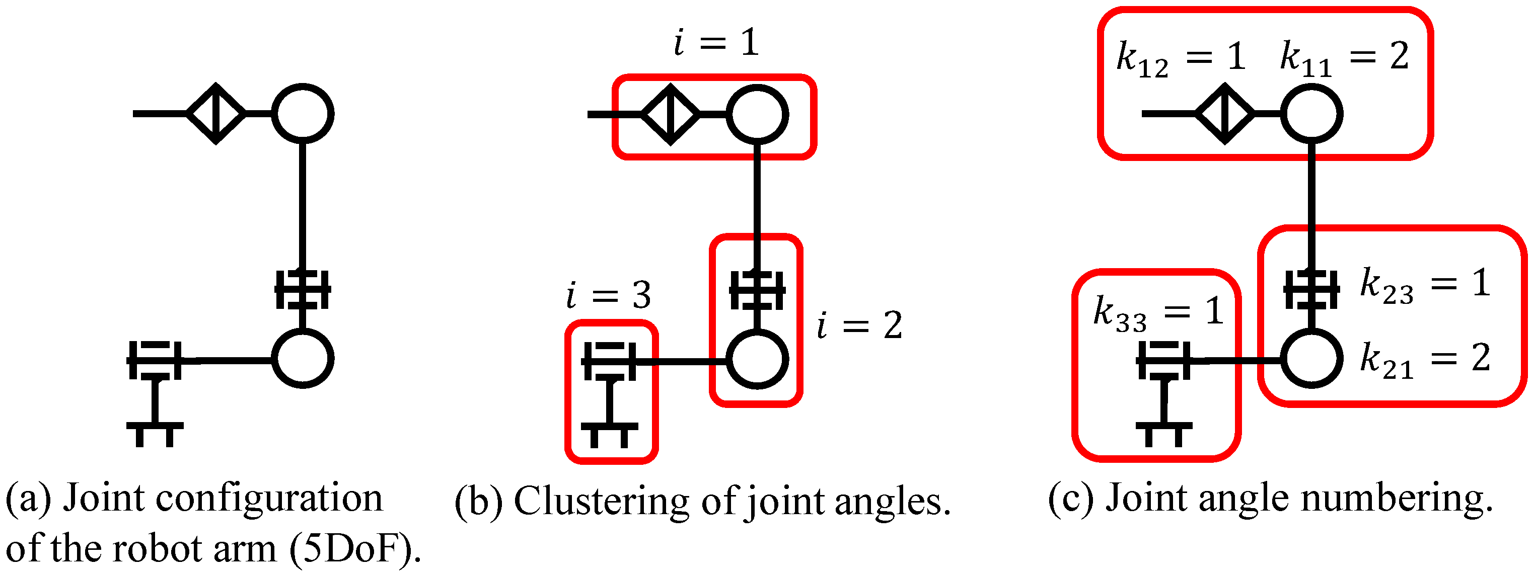
Figure 6a illustrates the joint model of a 5 DoFs robotic arm. As shown in Figure 6b, the arm is divided into three joint units according to the clustering rule described earlier. In Figure 6c, each element of the joint matrix is numbered sequentially from the base link to the end-effector, following the defined indexing rule.
Let the 5 DoFs robot’s joint matrix and joint angle vector be denoted by K r o b o t 1 and q r o b o t 1 , respectively; they are defined as
K r o b o t 1 = 0 1 2 1 0 2 1 0 0 , q r o b o t 1 = [ θ 1 r 1 θ 2 r 1 θ 3 r 1 θ 4 r 1 θ 5 r 1 ] T .
For this robot, the joint angle matrix Q r o b o t 1 is given by
Q r o b o t 1 = 0 θ 1 r 1 θ 2 r 1 θ 3 r 1 0 θ 4 r 1 θ 5 r 1 0 0 .
By comparing Equation (6) and Equation (8), the correspondence between the joint angle vector of the human arm and that of the robot can be established as follows:
q h u m a n = [ 0 θ 1 r 1 θ 2 r 1 θ 3 r 1 θ 4 r 1 0 0 ] T ,
q r o b o t 1 = [ θ 2 h θ 3 h θ 4 h θ 5 h 0 ] T .
Therefore, by constructing a joint angle matrix from a joint-angle vector using the joint matrix, and then comparing the Joint Angle Matrices of the demonstrator and the robot, the corresponding joint-angle vector can be derived. When the target robot does not have a corresponding joint, its element is masked with zero as in Equation (10). Such missing joint angles are later compensated through the imitation kinematics described in the following Section 3.3.3.
Previously, we described a method for transforming joint configurations using the joint matrix when the demonstrator and the robot have the same number of joint units. However, when their numbers of joint units differ, the row dimensions of the Joint Matrices become inconsistent, and the same transformation cannot be applied directly. In such cases, it is necessary to perform a transformation that aligns the dimensions of the two Joint Matrices.
Specifically, the joint matrix with fewer joint units is expanded along the column direction to match the dimension of the robot’s matrix with more units. Because the joint matrix preserves the correspondence between the joint angle matrix and the joint-angle vector, simply reducing the number of units would disrupt this relationship. Removing a unit would cause loss of certain joint angles, while merging units would make it impossible to distinguish multiple joint angles along the same axis. In either case, some joint configurations would become unreconstructable.
To resolve this issue, we introduce a virtual fixed joint unit defined as k = [ 0 , 0 , 0 ] . By inserting such units into appropriate columns to compensate for the difference in joint-unit numbers, the column dimension can be matched. Since the virtual fixed joint unit has no degrees of freedom on any rotational axis, adding it does not alter the robot’s kinematic structure. Furthermore, because these virtual fixed joints can be ignored in computation, the conversions between the joint angle matrix and the joint-angle vector remain consistent and complete.
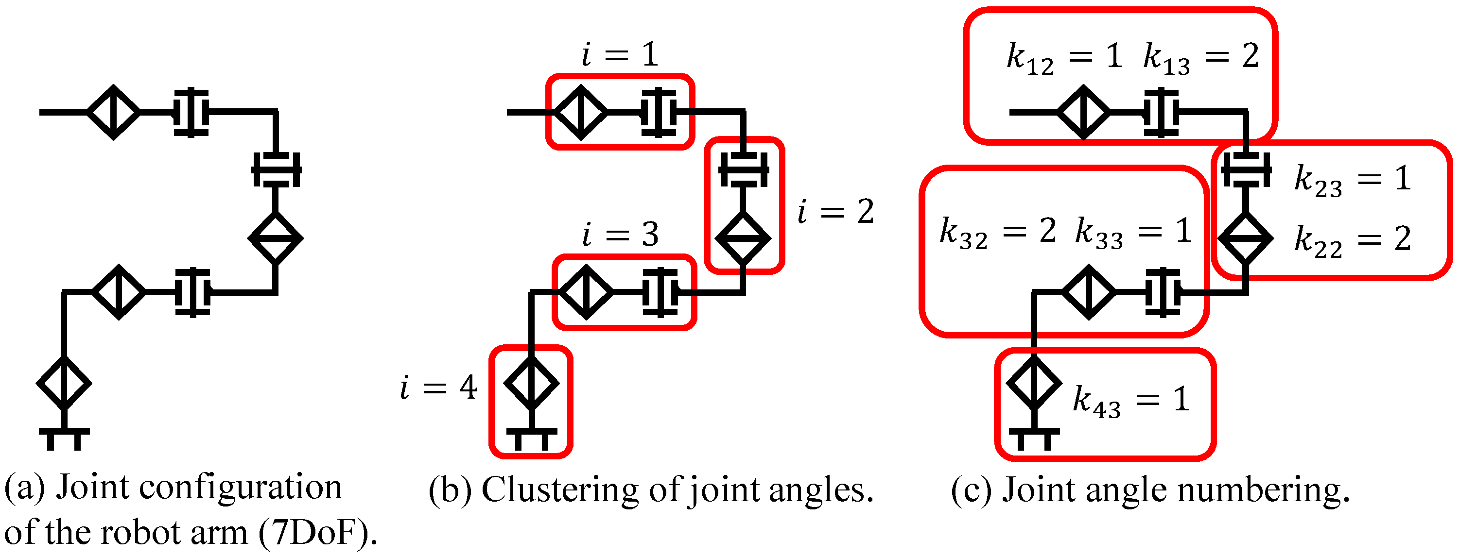
To illustrate the concept, we consider a 7 DoFs robotic arm model, as shown in Figure 7a. As depicted in Figure 7b, the arm is divided into four joint units according to the clustering rule described earlier. In Figure 7c, each element of the joint matrix is numbered sequentially from the base link to the end-effector, following the defined indexing rule.
Let the 7 DoFs robot’s joint matrix and joint angle vector be denoted by K r o b o t 2 and q r o b o t 2 , respectively; they are defined as
K r o b o t 2 = 0 1 2 0 1 2 0 1 2 0 0 1 , q r o b o t 2 = [ θ 1 r 2 θ 2 r 2 θ 3 r 2 θ 4 r 2 θ 5 r 2 θ 6 r 2 θ 7 r 2 ] T .
For this robot, the joint angle matrix Q r o b o t 2 is given by
Q r o b o t 2 = 0 θ 1 r 2 θ 2 r 2 0 θ 3 r 2 θ 4 r 2 0 θ 5 r 2 θ 6 r 2 0 0 θ 7 r 2 .
In this case, the demonstrator (human) has three joint units, whereas the teaching robot has four. To bridge this structural difference, a virtual fixed joint unit is inserted into the demonstrator’s joint matrix. This virtual joint unit is inserted such that the elements of the demonstrator’s joint matrix best correspond to those of the robot’s joint matrix. Therefore, it is necessary to quantitatively evaluate the correspondence between the two joint matrices based on their common elements.
To evaluate the compatibility of joint matrix, we define a new unit joint matrix C as follows:
f u ( k i j ) = 1 ( k i j > 0 ) 0 ( k i j = 0 ) ,
C = f u ( K ) .
Then, the compatibility between Joint Matrices can be evaluated by the Hadamard product of the unit joint Matrix of the larger joint matrix, C t a r g e t , and the unit joint matrix of the expanded joint matrix with inserted fixed joints, C e x p a n d . This compatibility is defined as
C g a p = C t a r g e t C e x p a n d ,
G j o i n t = i , j C i , j g a p .
According to Equation (15), the matrix C g a p retains a value of 1 in the elements where C t a r g e t and C e x p a n d share the same joint angles. Then, as shown in Equation (16), taking the summation over C g a p yields the total number of common joint angles. In this way, the virtual fixed joint units can be inserted such that the number of common joint angles is maximized.
Here, selecting the insertion location that maximizes the number of common joint axes ensures the highest structural correspondence between embodiments. In other words, the optimal virtual joint unit location is defined as the configuration that preserves joint motion correspondence as much as possible, thereby minimizing kinematic inconsistency introduced by embodiment differences.
We consider the case of a human and a 7DoF robotic arm, as illustrated in Figure 5a and Figure 7a. In this case, as shown in Equations (6) and (12), the number of joint units differs between the human and the robot, resulting in different column dimensions in their joint matrices. Therefore, one virtual fixed joint unit is inserted as an additional column. According to Equation (14), the extended human joint matrix C h is represented as shown by
C h = 0 0 0 1 1 1 1 0 1 0 1 1 , 1 1 1 0 0 0 1 0 1 0 1 1 , 1 1 1 1 0 1 0 0 0 0 1 1 , 1 1 1 1 0 1 0 1 1 0 0 0 .
Similarly, the joint matrix of the 7DoF robot, denoted as C r 2 , is shown by
C r 2 = 0 1 1 0 1 1 0 1 1 0 0 1 .
Based on Equations (15) and (16), Equations (17) and (18) are compared, and the resulting G j o i n t is shown by
G j o i n t = 4 , 4 , 4 , 5 .
From this result, the joint angle matrix is generated using the extended joint matrix in which the number of common joint angles is maximized. The conversion of the joint angle matrix Q r o b o t 2 and joint angle vector q r o b o t 2 from the human to the robot is expressed as follows:
Q r o b o t 2 = 0 θ 2 h θ 3 h 0 0 θ 5 h 0 θ 6 h θ 7 h 0 0 0 , q r o b o t 2 = [ θ 2 h , θ 3 h , 0 , θ 5 h , θ 6 h , θ 7 h , 0 ] .
In this way, even when the dimensions of the joint matrices differ, it is possible to evaluate them and generate a corresponding joint angle matrix. This formulation allows the joint matrix to represent kinematic structures even when the human and robot have different numbers of degrees of freedom (DOF) or the joint units. Therefore, the proposed method can handle embodiment differences both in joint count and joint motion capabilities, enabling consistent motion mapping across robots with different embodiments.

3.3.3. Imitation Kinematics for Imitation Learning

In this study, we employ Imitation Kinematics [8] to separate imitation motions according to the embodiment of the robot. Through the aforementioned transformations, the demonstrator’s motion is converted into a motion adapted to the robot’s body structure, yielding time-series data of the robot’s target end-effector pose x target and target joint angles q target . At this stage, two issues arise:
  • Due to the embodiment gaps, it is unlikely that a robot state exists that simultaneously satisfies both the target end-effector pose and the target joint angles.
  • In q target , the joint angles that do not exist in the demonstrator are set to 0 [rad].
To address these issues, both forward kinematics (FK) and inverse kinematics (IK) are solved numerically. In conventional FK, the end-effector pose corresponding to the robot’s target joint angles can be computed analytically. Similarly, IK can be solved either by geometric methods yielding analytical solutions, or by numerical approaches such as Newton’s method. However, in this study, both the target joint angles and target end-effector pose are given simultaneously. As a result, conventional FK and IK lead to inconsistencies between the solutions of the end-effector pose and joint angles due to embodiment gaps. Therefore, not only IK but also FK are solved numerically.
For this purpose, the Levenberg–Marquardt (LM) method is adopted. The LM method is a representative approach for nonlinear least squares problems, combining the advantages of the Gauss–Newton method and gradient descent, and is known for its relatively stable convergence even when the Jacobian is ill-conditioned. In this study, both IK and FK are realized by minimizing the following cost functions using the LM method:
V x = 1 2 ( x ^ · J q · ) T ( x ^ · J q · ) + λ x 2 q · T q · ,
V q = 1 2 ( x · J q ^ · ) T ( x · J q ^ · ) + λ q 2 x · T x · .
In the cost function for inverse kinematics given in Equation (21), x · denotes the end-effector velocity, q · represents the joint velocity, and J is the Jacobian matrix that maps joint velocities to end-effector velocities. The term x ^ is defined as the deviation between the target end-effector pose and the current end-effector pose. The regularization term λ x is introduced to minimize joint displacements, thereby ensuring stable solutions even in the vicinity of singular configurations. In the cost function for forward kinematics given in Equation (22), q ^ is defined as the difference between the target joint angles and the current joint angles. The regularization term λ q is used to suppress variations in the end-effector pose. Then, the gradients of the end-effector pose and joint angles that decrease V x and V q , respectively, are given as follows:
d q = ( J T J + λ x I ) 1 J T d x
d x = ( I + λ q I ) 1 J d q
Imitation kinematics first solves the standard inverse kinematics and then gradually modifies the target end-effector pose toward the target joint angles. The overall procedure of imitation kinematics is shown in Algorithm 1. Before each LM update, a few steps of Adam optimization [36] are applied to warm-start the joint configuration. This warm-start helps the solver escape highly nonlinear or ill-conditioned regions and brings the estimate into a locally convex region where the LM method converges more reliably. In particular, for robots with strong embodiment differences, this hybrid Adam-LM approach prevents divergence and improves numerical stability.
Algorithm 1 Imitation Kinematics
Require: 
x target , q target
Ensure: 
q I K , q I M K , x I K , x I M K
1:
 while not converged Δ q  do
2:
    while not converged Δ x  do
3:
        Calculate FK and Jacobian J
4:
         Δ x = x target x
5:
         q Adam ( | | Δ x ( q ) | | 2 )
6:
         Δ q = ( J T J + λ x I ) 1 J T Δ x
7:
         q q + η x Δ q
8:
        store q I K , x I K
9:
      end while
10:
    Calculate Jacobian J
11:
     q target is given by the joint angle matrix
12:
     d q = q target q
13:
     Δ x = ( I + λ q I ) 1 J Δ q
14:
     x t a r g e t x + η q Δ x
15:
    store q I M K , x I M K
16:
end while
First, following the gradient in Equation (23), the standard inverse kinematics is solved using the LM method to obtain joint angles that approximately satisfy the target end-effector pose. Next, according to the gradient in Equation (24), the target end-effector pose is gradually shifted toward one that satisfies the target joint angles. By repeating this process, the joint angles are explored to maximize the consistency between the end-effector pose and the joint angles, rather than to minimize both errors to zero. Finally, the solutions considered are the joint angles taken as close to the target end-effector pose, denoted as q I K , and those taken as close to the target joint angles, denoted as q I M K . Their corresponding end-effector poses are x I K and x I M K , respectively. Here, IMK stands for Inverse Matrix Kinematics.
In the zero mask for the joint matrix, elements that do not exist in the robot’s implementation are set to zero.
Note that zero-masked joint angles are treated as free variables and are automatically estimated through the IMK optimization using the Levenberg–Marquardt algorithm. During this process, the optimizer updates the missing joint angles so as to minimize the discrepancy between the robot’s kinematics and the demonstrated human motion, thereby compensating for structural differences while respecting the robot’s kinematic constraints.
In Algorithm 1, the target joint angle vector q target is obtained through the joint angle matrix. q target directly reflects the common joint angles between the demonstrator and the robot, as defined in Equation (10). The joint angles derived from Equation (10) can be applied without issue when the human and robot share identical or similar kinematic structures. However, if their joint configurations differ, the resulting motion deviates significantly. Therefore, by treating the joint angles obtained from Equation (10) as an initial solution and solving the imitation kinematics described in Algorithm 1, the robot’s motion can be efficiently reconstructed in accordance with its own embodiment. The learning process is conducted using the joint trajectories q I K , q I M K obtained through Algorithm 1.

3.4. Learning Embodiment and Imitative Movement

3.4.1. Evaluation of Compatibility by Energy-Based Model

In this study, we employ an Energy-Based Model (EBM) [6] as the policy model. This model enables the evaluation of embodiment gaps between the demonstrator and the robot, and facilitates imitation. An EBM learns the compatibility between two inputs through an energy function: when the two inputs are highly compatible, the model outputs low energy; when they are incompatible, it outputs high energy.
Based on this principle, we train an EBM to model the demonstrator’s embodiment. By feeding the robot’s embodiment information into this trained model, we can evaluate the compatibility between the demonstrator and the robot, interpreting embodiment gaps as incompatibilities in energy space.
Furthermore, Imitation by Energy-Based Models (IBC) [7] has shown that imitation policies can also be learned using EBMs, achieving strong performance in highly nonlinear control tasks. Inspired by this approach, we also adopt an EBM to learn the imitation policy model in this work. In IBC, the demonstrator’s behavior is represented as a state–action relationship, and the EBM learns the compatibility between states and actions. Imitation is realized by inferring the action that yields the lowest energy (i.e., the highest compatibility) for the robot’s current state.
In this study, we extend the IBC framework to jointly train two EBMs: one for the demonstrator’s embodiment model and another for the robot’s imitation policy model. The following subsection outlines the learning procedure of IBC. Let E ( s , a ) denote a neural network that outputs the energy corresponding to a given state s and action a . Then, the conditional distribution P ( a | s ) is defined as follows:
P ( a | s ) = e E ( s , a ) Z .
Here, Z denotes the partition function, which normalizes the conditional probability P ( a | s ) . However, computing Z analytically is generally intractable. Therefore, we approximate Z by randomly sampling N neg negative actions a ˜ , as follows:
Z e E ( s , a ) + j = 1 N n e g e E ( s , a ˜ j ) .
In this approximation, the first term is computed using the energy of the demonstrator’s state–action pair ( s , a ) , while the second term is computed using the same state s paired with a negative (counterexample) action a ˜ . Because a ˜ does not appear in the demonstration data, it is treated as a counterexample action. Using this approximation of Z, the conditional probability P ( a | s ) can be rewritten as follows:
P ( a | s , { a ˜ } N n e g ) = e E ( s , a ) e E ( s , a ) + j = 1 N n e g e E ( s , a ˜ j ) .
Then, using the approximately normalized distribution P ( a | s , { a ˜ } N n e g ) , the parameters of E ( s , a ) are updated so as to minimize the following InfoNCE-style loss function:
L I n f o N C E = i = 1 N log P ( a | s , { a ˜ } N n e g ) .
In this context, NCE in InfoNCE stands for Noise Contrastive Estimation, a loss function used in contrastive learning with negative actions. Equation (28) can thus be interpreted as maximizing the conditional probability P ( a | s , { a ˜ } N neg ) for the demonstrator’s state–action pairs ( s , a ) .
During imitation, the optimal action is inferred by solving the following minimization problem based on the learned energy function E ( s , a ) :
a * = argmin a E θ ( s , a ) .
The minimization problem is solved using Importance Sampling to infer the optimal action, as described in Algorithm 2. Specifically, a set of candidate actions a sample is first generated based on the mean action at each timestep of the demonstration data. Among these candidates, the action with the lowest energy is selected as the initial estimate. This estimated action is then duplicated N sample times, and Gaussian noise drawn from N ( 0 , σ ) is added to each copy. From the resulting noisy actions, the one with the lowest energy is again selected. By iteratively repeating this procedure, the algorithm refines the action estimate toward lower energy, thereby improving the imitation performance.
Algorithm 2 Importance Sampling
Require: 
s , { a } sample
Ensure: 
a *
1:
for  i = 1 , , N iter do
2:
     a ^ argmin a { a } sample E ( s , a )
3:
     { a } N sample replicate ( a ^ , N sample )
4:
     { a } N sample { a ^ } N sample + N ( 0 , σ )
5:
     σ k σ
6:
     { a } sample { a } N sample
7:
     a * argmin a { a } sample E ( s , a )
8:
end for

3.4.2. Embodiment Model of Demonstrator and Imitative Movement Model of Robot

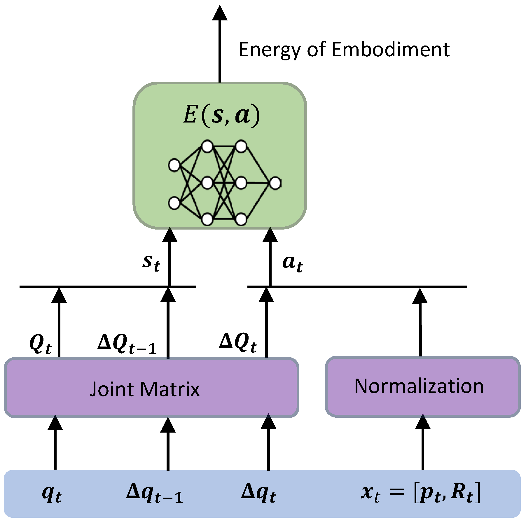
First, the demonstrator’s embodiment and the ideal imitation behavior are learned using an EBM. To apply the learning rule of IBC, the EBM is formulated to learn a state–action model of the demonstrator. The state s t and action a t are defined as follows:
s t = ( Q t , Q t Q t 1 ) , a t = ( x t , Q t + 1 Q t ) .
The state is defined by the joint angle matrix Q t together with its displacement from the previous timestep ( Q t Q t 1 ) . This displacement term is introduced to preserve the Markov property in the state–action model. The action is defined by the end-effector pose x t = [ p t , R t ] and the displacement toward the target joint angle matrix ( Q t + 1 Q t ) . The overall input structure of the embodiment model, including these transformations, is illustrated in Figure 8.
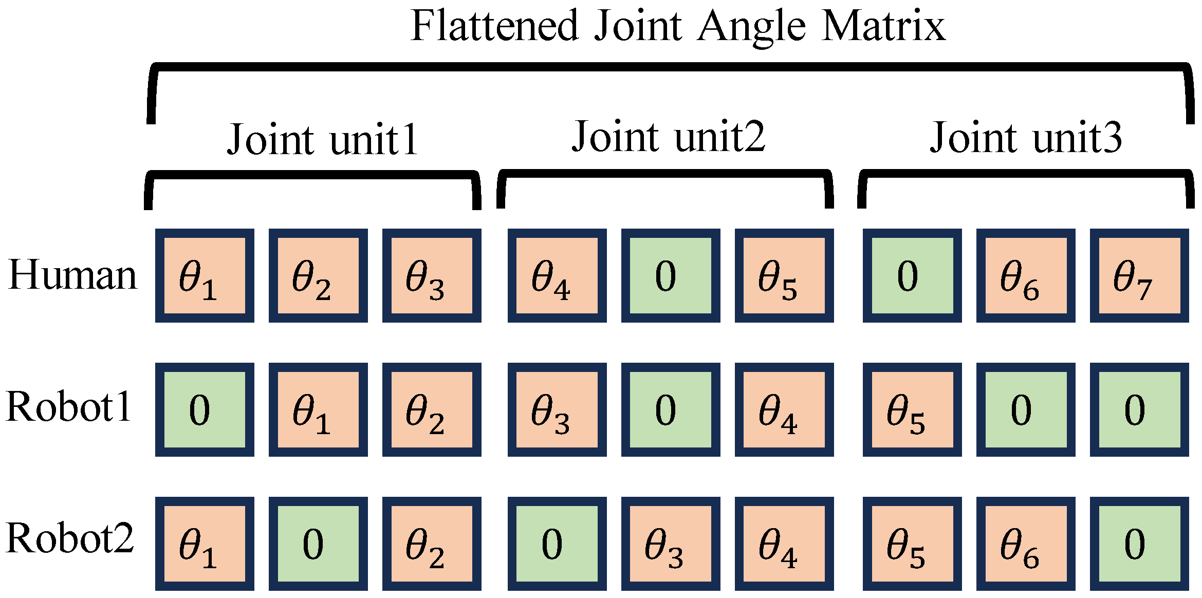
A key design concept of this formulation is the use of the joint angle matrix Q t instead of the conventional joint angle vector q t . In this representation, the zeros in Q t serve as padding masks, introducing redundancy that allows the trained model to process inputs from robots with different kinematic structures. The role of the joint angle matrix in providing this flexibility is illustrated in Figure 9.
With the above definitions of state and action, the embodiment model learns two types of compatibilities: (1) between joint angles and end-effector poses, and (2) between joint angles and target joint angles. Learning the former enables the model to acquire an understanding of the demonstrator’s embodiment, while learning the latter allows it to simultaneously develop an ideal imitation behavior model that reproduces the demonstrator’s motion.
Furthermore, by inputting the transformed motions—adapted from the demonstrator to the robot’s embodiment—into the trained embodiment model, the estimated energy can be used to evaluate both embodiment compatibility and imitation compatibility. Extending this evaluation to different robots or body parts makes it possible to determine which robot possesses an embodiment most similar to the demonstrator, and which robot can achieve the most faithful imitation behavior.
Unlike conventional approaches that rely heavily on human subjectivity, the proposed embodiment model provides a quantitative framework for evaluating both embodiment gaps and imitation performance. This enables an objective, numerical assessment of how closely each robot replicates the demonstrator’s embodiment and behavior.
Next, the imitation behavior model for the robot is trained using an EBM. Following the learning rule of Implicit Behavioral Cloning (IBC), the EBM is formulated as a state–action model for the robot, in the same manner as the embodiment model. The state s t and action a t are defined as follows:
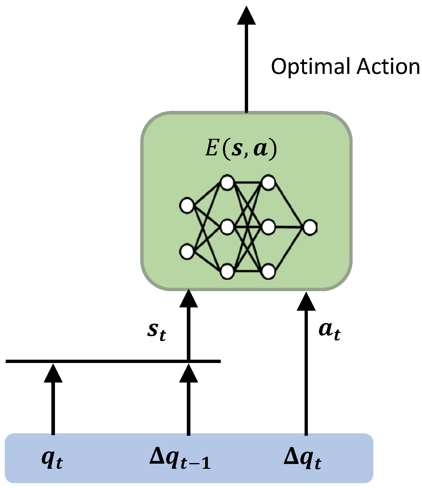
s t = ( q t , q t q t 1 ) , a t = ( q t + 1 q t ) .
The state is defined by the joint angle vector q t together with its displacement from the previous timestep ( q t q t 1 ) . The inclusion of this displacement term ensures the Markov property of the state–action model. The action is defined as the displacement toward the target joint angle vector, ( q t + 1 q t ) . The input structure of the imitation behavior model is illustrated in Figure 10.
In both the embodiment model and the imitation motion model, the energy function E is represented by a Multi-Layer Perceptron (MLP), as shown in
E = MLP ( dim hid , Layers ) .
In this context, dim hid denotes the dimension of the hidden layer, and Layers represents the number of hidden layers. The activation function used is Leaky ReLU.
In IBC, a known challenge is that the estimation of imitation behaviors becomes unstable as the dimensionality of the action space increases. To address this issue, the action is restricted to the minimal representation of the joint angle vector. With this definition of states and actions, the imitation behavior model learns the compatibility between joint angles and target joint angles. By capturing this compatibility, the robot can acquire joint angle trajectories that are suitable for imitation, forming its imitation behavior model.

4. Imitation Learning Considering Embodiment Gap Using X-EKBC

4.1. Motion Reconstruction Using Joint Matrices

To verify whether the proposed joint angle matrix (JAM) successfully reconstructs human motion, we conducted an experiment in which a human subject draws a circle with the right arm. We selected a circle-drawing task because circular motion requires coordinated control of multiple joints and continuous curvature change. Successfully reproducing such a trajectory demonstrates the robot’s capability to reconstruct a wide range of human arm movements while adapting to its own embodiment. Therefore, this task is well suited for evaluating embodiment-aware motion imitation.
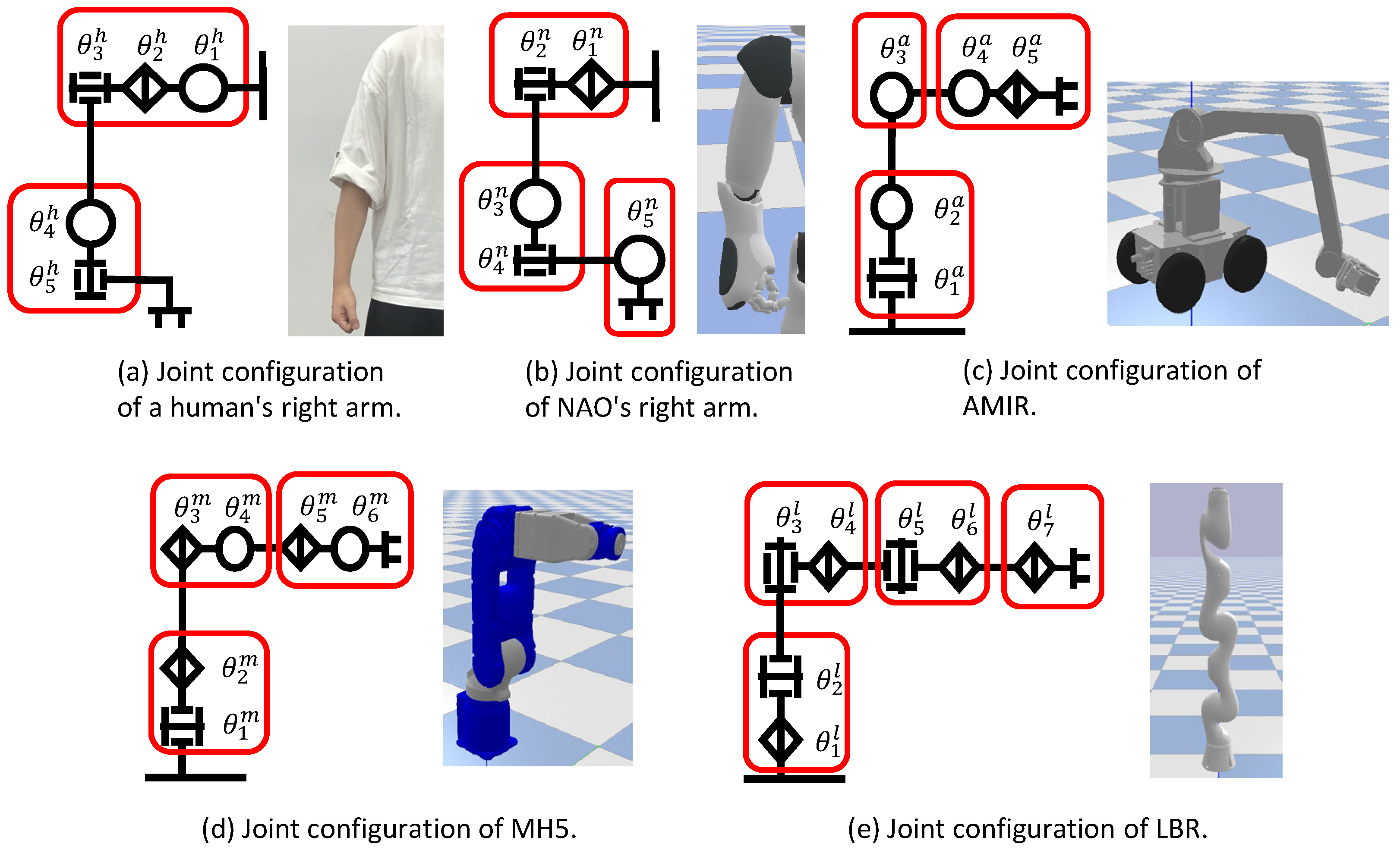
The robots used in this study are the NAO V6 (NAO, SoftBank Robotics), AMIR740 (AMIR, Vstone), MOTOMAN MH5 (MH5, Yaskawa Electric), and LBR iiwa 14 r820 (LBR, KUKA). The human, NAO, and AMIR each have 5 degrees of freedom (DoFs), MH5 has 6 DoFs, and LBR has 7 DoFs.
Figure 11 shows the joint angle configurations of the human and the four robots. Based on Figure 11, the joint-angle matrices of the human and the robot are represented as
Q h u m a n = θ 1 h θ 2 h θ 3 h θ 4 h 0 θ 5 h , Q N A O = 0 θ 1 n θ 2 n θ 3 n 0 θ 4 n θ 5 n 0 0 , Q A M I R = θ 2 a 0 θ 1 a θ 3 a 0 0 θ 4 a θ 5 a 0 , Q M H 5 = 0 θ 2 m θ 1 m θ 4 m θ 3 m 0 θ 6 m θ 5 m 0 , Q L B R = 0 θ 2 l θ 1 l 0 θ 4 l θ 3 l 0 θ 6 l θ 5 l 0 0 θ 7 l .
Here, θ h , θ n , θ a , θ m , θ l correspond to parameters human, NAO, AMIR, MH5 and LBR, respectively. In addition, since the wrist motion tends to be unstable during pose estimation, the human model is defined with five degrees of freedom.
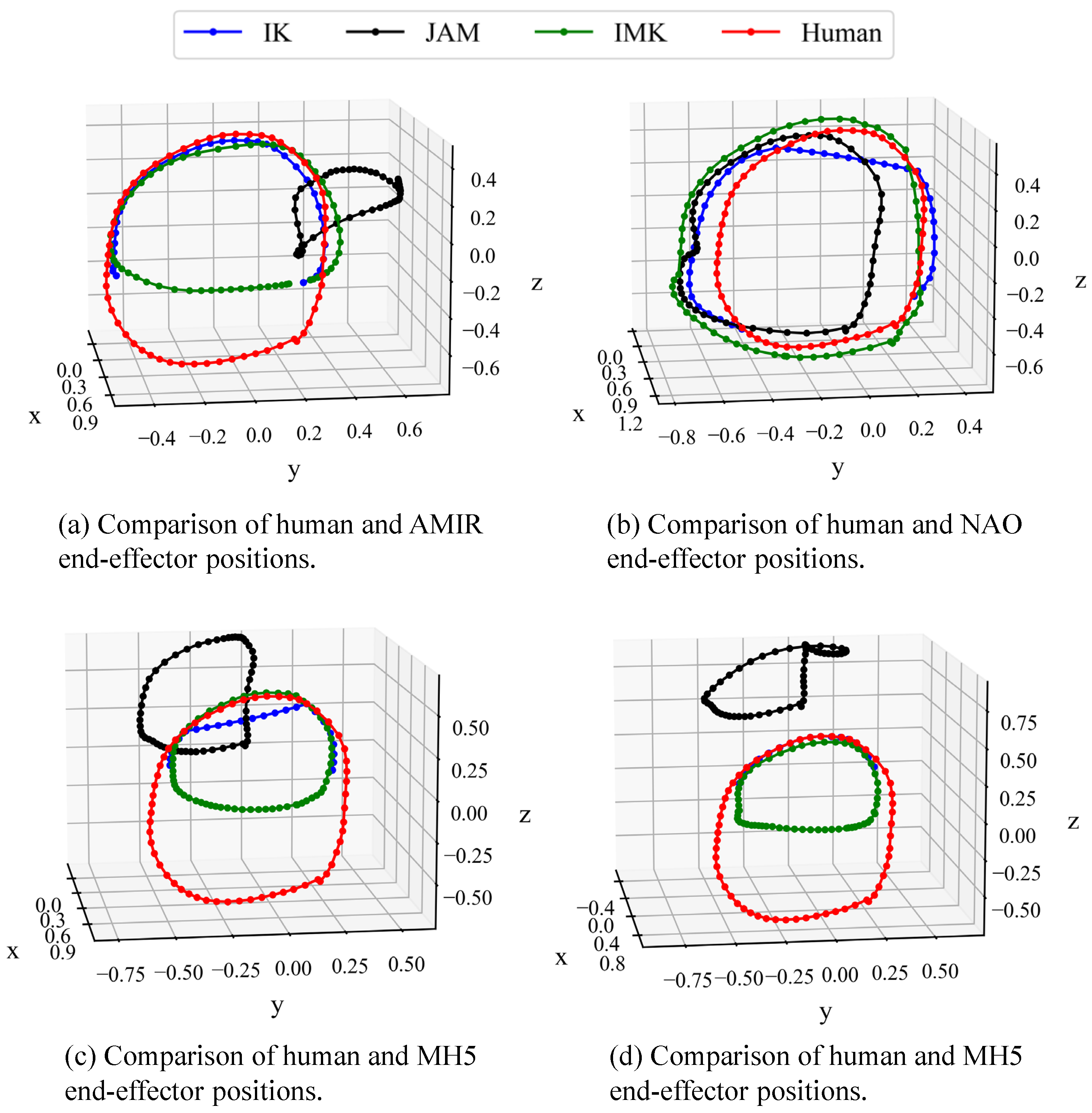
In this study, we compare three types of motion reconstruction methods. The first, denoted as x I K , reconstructs motion by solving inverse kinematics with a focus solely on the end-effector position. The second, x J A M , directly transfers the human joint angles to the robot without considering structural differences. The third, x I M K , reconstructs motion using the proposed Imitation Kinematics framework based on the joint angle matrix.
Figure 12 shows the end-effector trajectories of the human and the reconstructed robot motions. As shown in Figure 12a, for AMIR, x I K fails to reconstruct the lower part of the circle where the robot cannot reach, while x J A M produces a trajectory that significantly deviates from a circular motion. In contrast, x I M K successfully reproduces a circular trajectory similar to that of the human, even in regions unreachable by AMIR. As shown in Figure 12b, since NAO has a body structure similar to that of the human, all three methods x I K , x J A M , and x I M K can reconstruct the circular motion. As shown in Figure 12c, for MH5, x I K fails to reproduce the lower circular region due to reachability limits, and x J A M generates a shifted trajectory. In contrast, x I M K achieves a circular trajectory comparable to the human’s motion, even in the unreachable region. As shown in Figure 12d, for LBR, x I K again fails to reconstruct the lower part of the circle, and x J A M results in a non-circular motion. Conversely, x I M K successfully reconstructs a human-like circular trajectory, including the lower region beyond LBR’s reachable workspace.
These results indicate that IMK effectively reconstructs human motion across robots with different kinematic structures. Thus, the proposed method is expected to generalize to various robots and motion types. Based on this result, imitation learning is performed using the joint angle trajectories q I M K through the EBM.
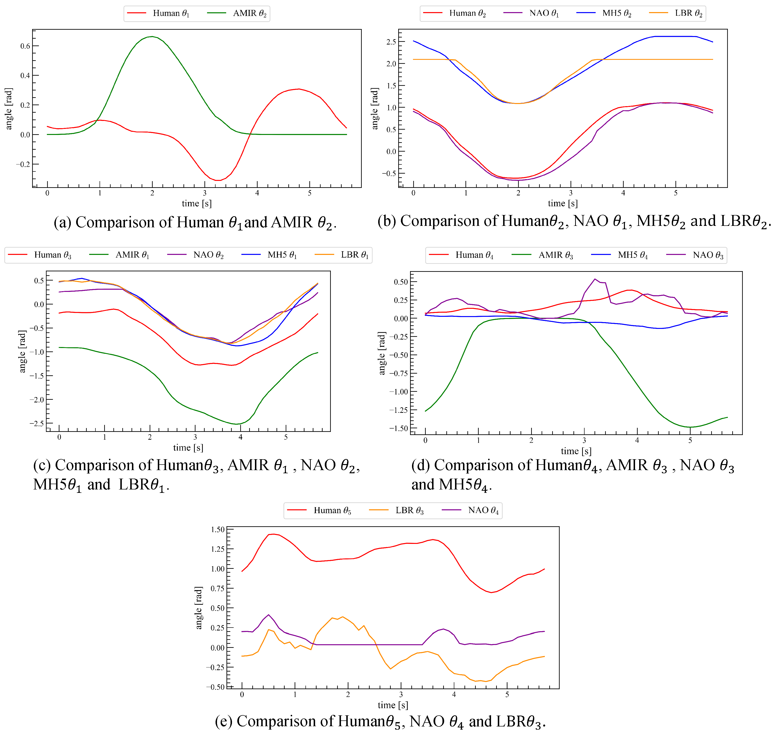
Figure 13 shows the joint angle transitions for x I M K . In Figure 13, Red indicates human joint angles, green represents AMIR angles, purple corresponds to NAO angles, blue shows MH5 angles, and orange denotes LBR angles. The correspondence between colors and robots remains the same in the following figures.
In Figure 13 the NAO, whose kinematic structure closely resembles that of the human, exhibits joint angle trajectories highly similar to the human’s. For MH5 and LBR, some joint trajectories align with the human’s, while others differ. For AMIR, all joint angles show clear divergence from the human’s trajectories.
From the results of Figure 12 and Figure 13, it is confirmed that motion reconstruction was successfully achieved for each robot. However, differences in end-effector trajectories and joint angles between human and robot alone do not allow us to determine whether the reconstructed motion is appropriate for imitation. Therefore, a quantitative evaluation of embodiment gaps between human and robot is required.
When embodiments differ, the reproduction of end-effector trajectories and joint-angle motions inherently forms a trade-off relationship. Consequently, the trajectory deviations observed in Figure 12 and Figure 13 could only be evaluated qualitatively in prior approaches.
In contrast, Section 4.2 introduces an Energy-Based Model (EBM), which enables a quantitative assessment of embodiment compatibility by incorporating end-effector trajectories, joint angles, and target joint angles trajectories into the energy evaluation.

4.2. Quantifying Embodiment Gap Through EBM

In conventional imitation learning research, evaluation metrics have primarily focused on task success rates and end-effector trajectory errors. However, in imitation learning across different embodiments, such metrics are insufficient because discrepancies in body structure prevent direct comparison in either end-effector space or joint-angle space alone. To address this limitation, we employ an EBM to quantitatively evaluate the overall motion compatibility between agents whether human-to-robot or robot-to-robot—by interpreting it as energy.
In this study, an EBM trained on human embodiment is used as a reference model. The embodiment models of four different robots are then input to the EBM, and the resulting energy differences are interpreted as quantitative measures of embodiment discrepancy. The model is trained using Equation (30). The joint angle matrix at this time uses Equation (33).
The EBM for learning the human embodiment representation was trained for 500 epochs with a learning rate of 0.001, a batch size of 256, dimension of the hidden layer of 256, number of hidden layers of 8.
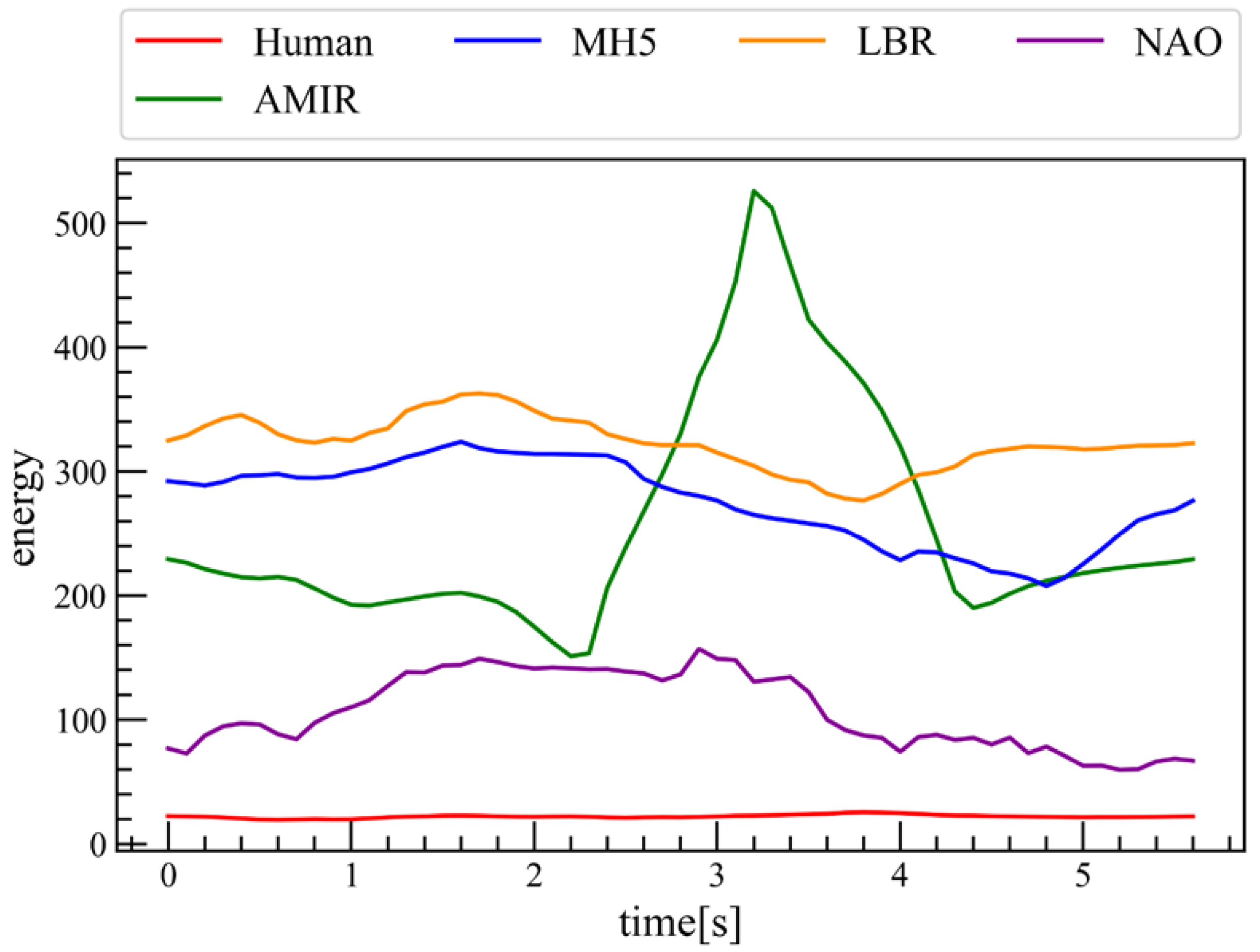
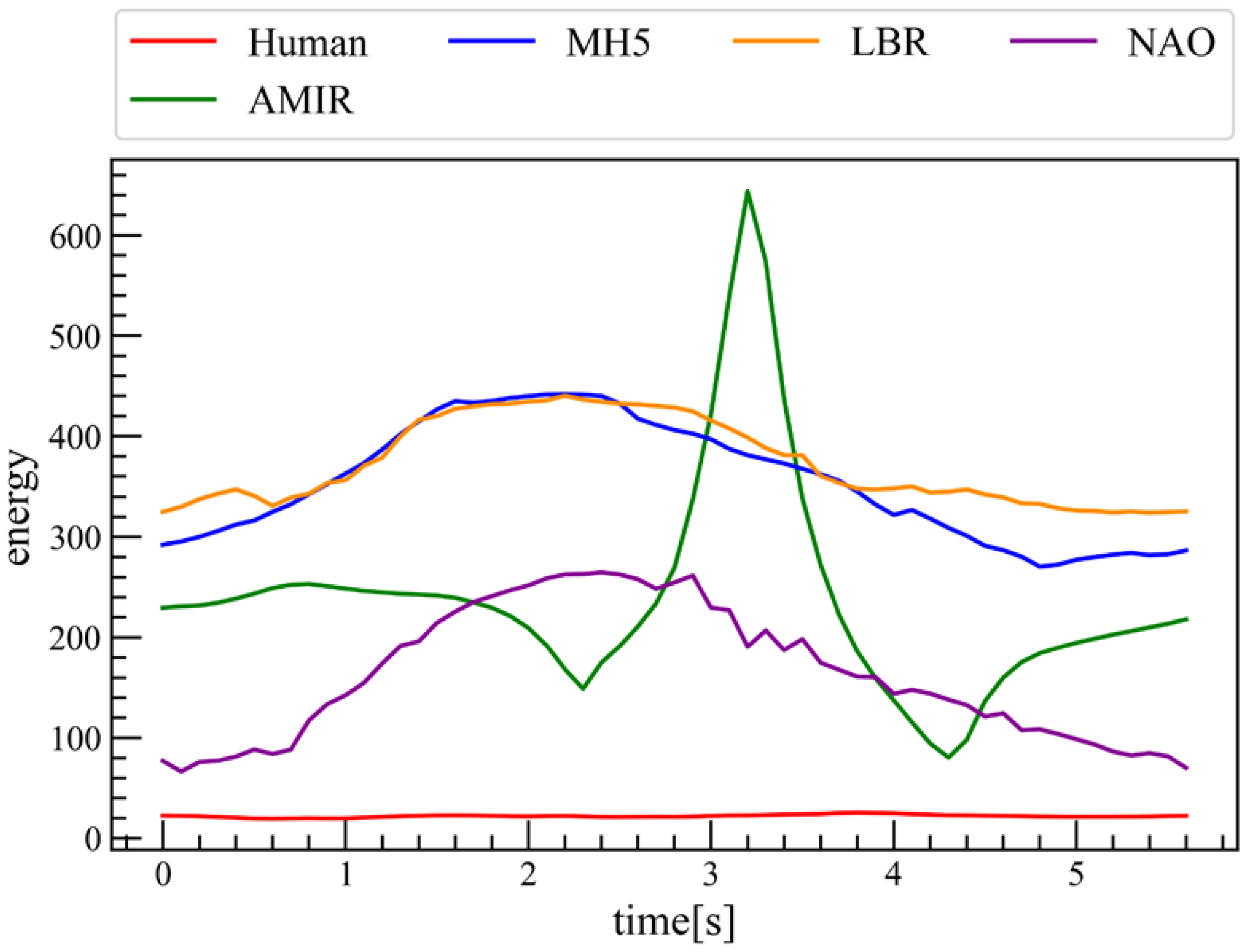
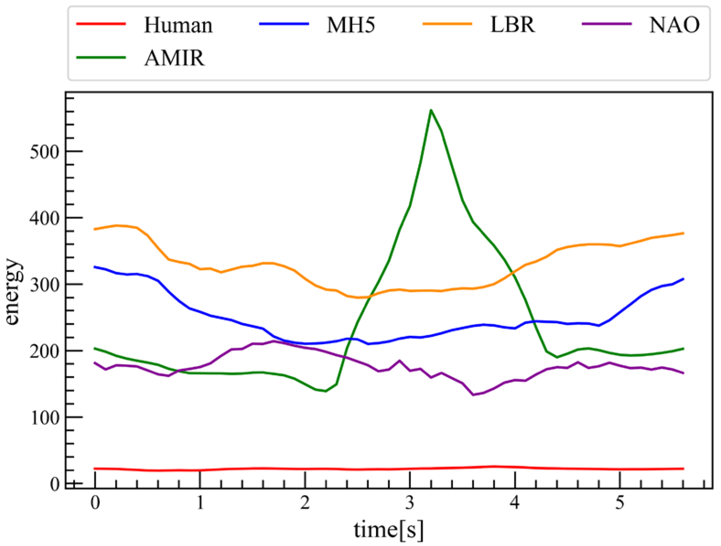
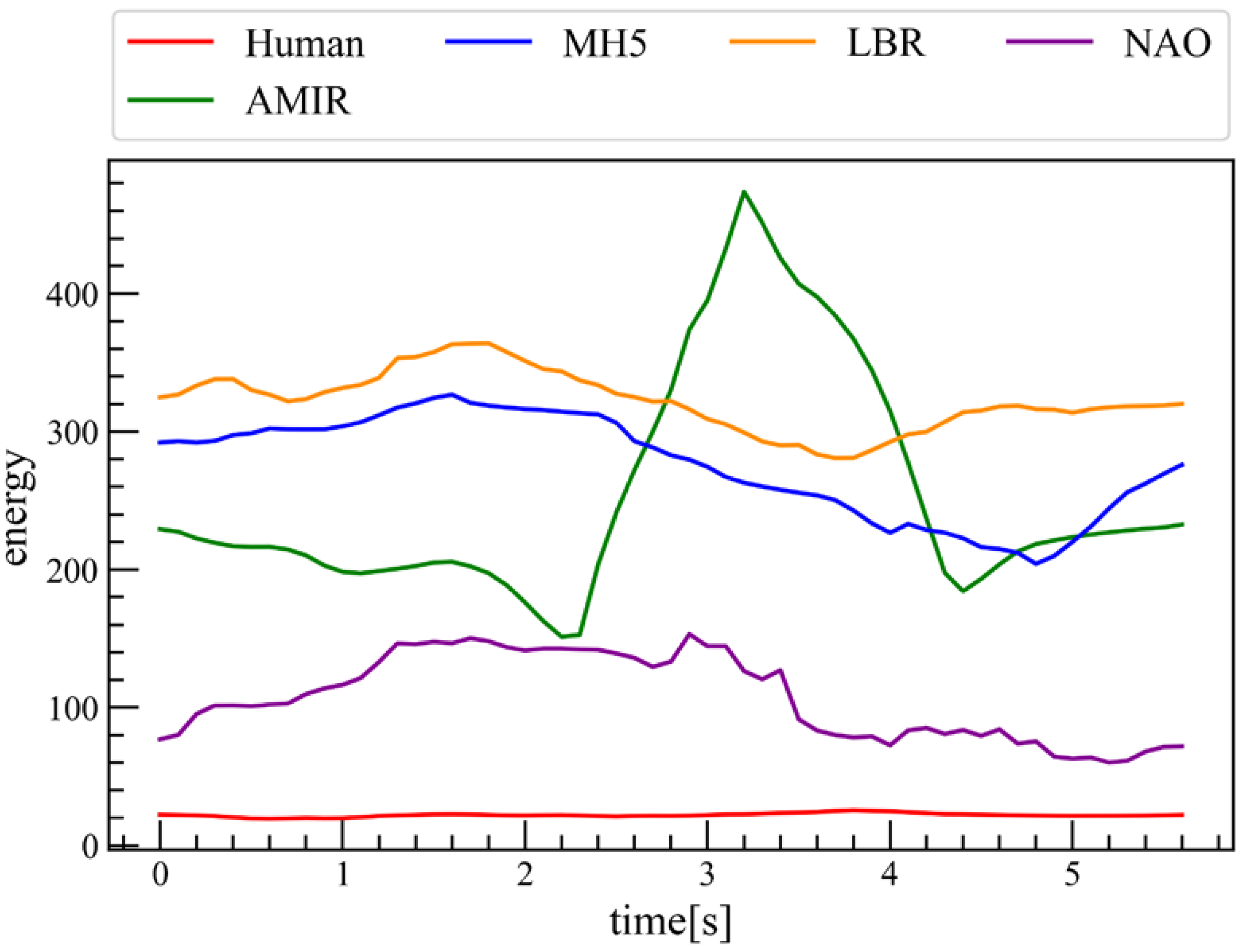
The energy output of the embodiment model represents the compatibility between the reproduced robot motion and the human demonstration, where lower energy indicates smaller embodiment gaps. While the absolute values of energy are not themselves meaningful, the relative difference from the human’s energy serves as an indicator of imitation discrepancy. In other words, the deviation of a robot’s energy from that of the human quantitatively reflects the magnitude of the embodiment gap. Therefore, the energy curves in Figure 14 provide a quantitative measure of embodiment similarity across robots during imitation. This interpretation also applies to the subsequent energy plots shown in Figure 15, Figure 16 and Figure 17.
In Figure 14, Figure 15, Figure 16 and Figure 17, the energy trajectories for each subject are shown: red for the human, blue for MH5, orange for LBR, purple for NAO, and green for AMIR. Since lower energy indicates a smaller embodiment gap, the relative differences among these colored curves allow a direct comparison of motion compatibility across embodiments.
We evaluate the embodiment gaps based on the reconstructed motions, with the energy outputs shown in Figure 14. Since the EBM was trained on human motion data, it outputs the lowest energy for human input, confirming that the model has been properly trained. Among the robots, NAO exhibits the lowest energy because its humanoid structure most closely resembles that of a human, indicating the smallest embodiment gap. AMIR shows the next lowest energy but displays a notable energy spike around three seconds, suggesting a momentary deviation in motion compatibility. MH5 records the second-highest average energy, while LBR yields the highest overall energy. This trend can be attributed to differences in the number of degrees of freedom MH5 having one more and LBR two more than the human model which likely increase structural divergence and, consequently, energy values.
To investigate the causes of elevated energy values, we conducted ablation tests by systematically removing information on joint angles, end-effector poses, and joint angular velocities. The results of these ablation studies are presented in Figure 15, Figure 16 and Figure 17, respectively.
Figure 15 shows the results of the joint-angle ablation test. When joint-angle information is removed, the energy increases significantly for all robots. The rise is particularly pronounced for NAO and AMIR, indicating that joint-angle information plays the most critical role in representing embodiment. This suggests that the EBM distinguishes embodiments primarily based on structural and dynamic characteristics of joint configurations.
Figure 16 shows the results of the end-effector pose ablation test. When pose information is removed, the overall energy increase is minor, implying that end-effector pose is not a dominant factor in determining embodiment gaps. Especially for humanoid robots such as NAO and AMIR, energy changes remain small even when the end-effector orientation deviates slightly.
Figure 17 presents the results of the joint-angular-velocity ablation test. When joint angular velocity or temporal transitions are removed, the energy moderately increases. This indicates that the smoothness and temporal pattern of motion also contribute to the EBM’s embodiment discrimination. Therefore, not only static joint structures but also dynamic features such as motion rhythm and acceleration are captured as important embodiment-related cues.
Next, we discuss the cause of the sharp energy increase observed for AMIR around 3 s. Based on the ablation results, the surge is primarily attributed to the joint-angle configuration and its rapid temporal variation, rather than to the end-effector pose. When joint-angle information is removed, the peak is largely suppressed, whereas removing pose information causes only minor change, and excluding transition (velocity) features results in a moderate reduction. This suggests that at the lower part of the circular trajectory, AMIR performs a compensatory posture adjustment due to its reach limitation, producing a joint configuration that differs from that of the human model. In particular, a noticeable bulge in certain joints (e.g., AMIR θ 3 in Figure 13d) and a transient rise in joint angular velocity were observed, both of which are assigned high energy by the EBM trained on human motion data. Hence, the spike originates from a non-human-like motion reconstruction caused by reach constraints, rather than from a simple mismatch in end-effector position.
From these results, it was demonstrated that the proposed method can quantitatively evaluate embodiment gaps not only through the trade-off relationship between joint angles and end-effector poses, but also by capturing the dynamic characteristics of the overall motion.

4.3. Imitation Learning with IBC

Imitation learning was conducted using the IBC framework. IBC addresses two major limitations of conventional BC. First, regarding the distribution shift problem, IBC mitigates performance degradation caused by unseen inputs through contrastive learning, which enhances generalization beyond the training distribution. Second, concerning the action averaging problem, IBC inherently models multi-modal distributions, thereby avoiding the averaging of multiple possible outputs. Given these characteristics, IBC is expected to be effective for imitation learning across heterogeneous embodiments, where motion distributions differ among agents.
In this study, we trained the IBC model using motion reconstructed by the proposed IMK as the teacher data. The input state–action pairs are defined by Equation (31), while the joint angles are represented as vectorized forms of Equation (33). By ensuring compatibility between joint angles and target joint angles, the model learns the joint trajectory generation for imitation.
The IBC models were trained individually for each robot. The number of training epochs was set to 500 for NAO, 340 for AMIR, 400 for MH5, and 600 for LBR. The learning rate was fixed at 0.001, the batch size was 256, the number of negative samples was 128, and the hyperparameters were set to k = 0.4 and σ = 0.3 . The simulations were conducted using the URDF models of each robot [37]. The simulation environments were implemented with PyBullet and qiBullet [38].
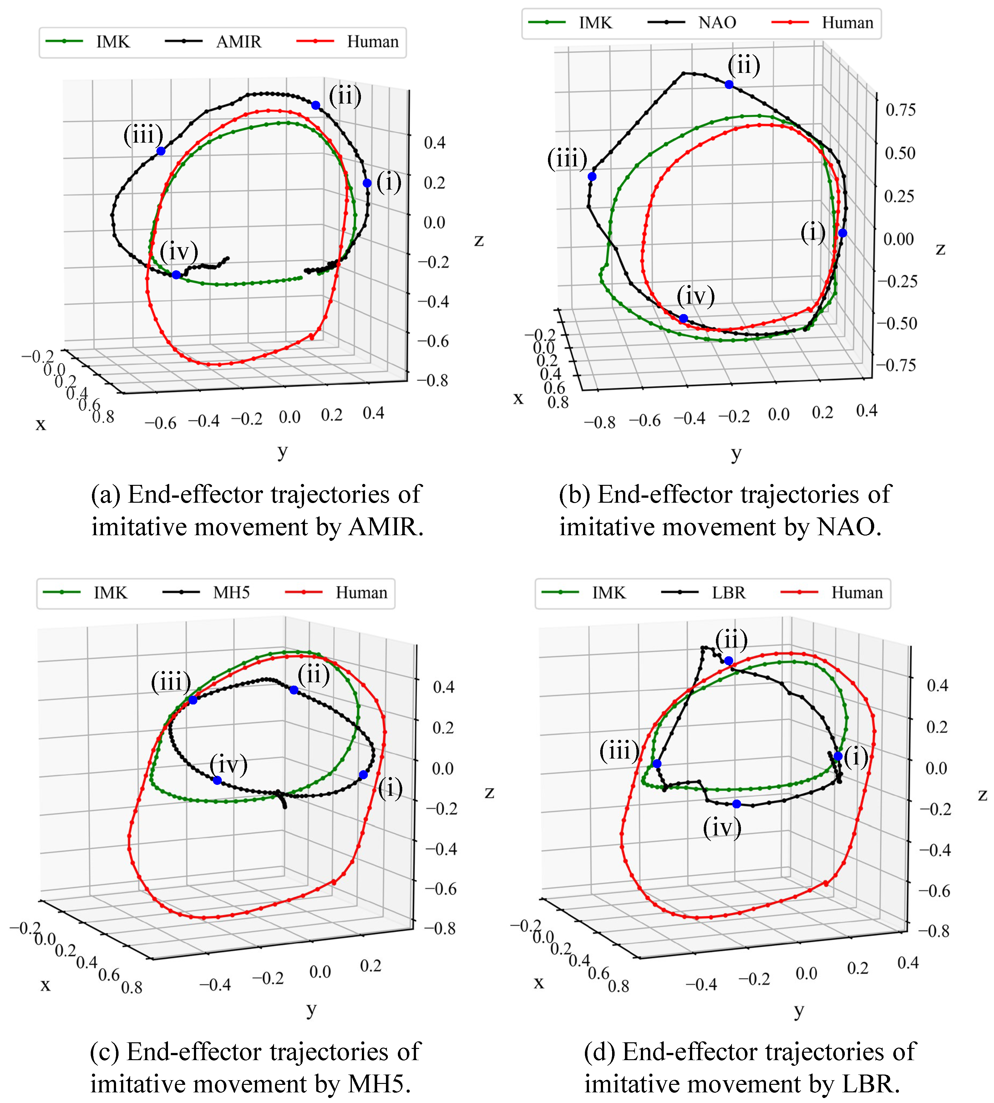
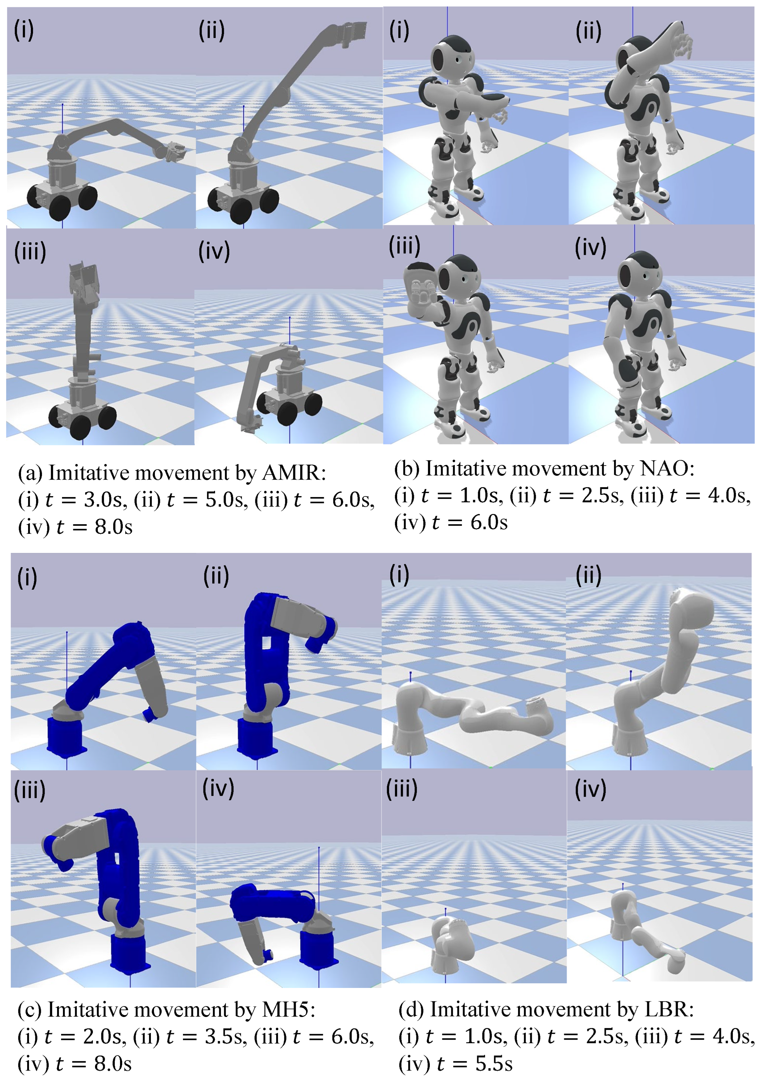
Figure 18 and Figure 19 show the resulting end-effector trajectories and corresponding imitation behaviors of the robots. In Figure 19, snapshots are extracted at the points (i)–(iv) indicated on the corresponding end-effector trajectories shown in Figure 18. The motion sequence (i)–(iv) follows the circular trajectory direction and confirms that the robots execute circle-drawing behavior.
As shown in Figure 18a, AMIR reproduces the trajectory learned from IMK with a nearly circular shape, although slight deviations appear in the lower part of the circle due to its reach limitation. In Figure 18b for NAO, the reproduced trajectory closely matches the IMK trajectory, achieving high consistency in both shape and smoothness. In the case of MH5 for Figure 18c, the circular motion pattern is preserved, but the trajectory shows a small spatial offset compared with the IMK reference, reflecting differences in arm configuration and range of motion. In Figure 18d, LBR also follows the IMK trajectory well, although slight discrepancies are observed in the lower region, likely caused by kinematic redundancy in its seven degrees of freedom.
These results indicate that the IBC model successfully learned the imitation policy from IMK-generated trajectories, reproducing them across robots with different kinematic structures. Because IMK explicitly encodes the correspondence between human and robot joint angles, it provides a consistent motion representation that serves as an effective teaching signal for IBC. The reproduced trajectories of NAO and AMIR show high similarity to the IMK reference, suggesting that for robots with relatively similar kinematics, IBC can accurately reproduce IMK-level motion quality. Although MH5 and LBR have more distinct kinematic structures, both maintain the overall circular trajectory, demonstrating that IBC effectively captures the essential features of IMK-based motion, even under embodiment gaps. These findings confirm that the combination of IMK and IBC allows for robust imitation learning based on kinematic correspondence, where IBC can reproduce the reference trajectories generated by IMK across heterogeneous robot embodiments.
In addition, the embodiment gaps of the imitation learning results were quantitatively evaluated using the EBM. Following the same procedure as in Section 4.2, the robot embodiment models—composed of joint angles, end-effector positions, and joint trajectories obtained from the imitation learning results—were input into the EBM that had been pre-trained on the human embodiment model (identical to the model used in Section 4.2). The energy output of the EBM was then used to evaluate the embodiment discrepancy between the human and the robots.
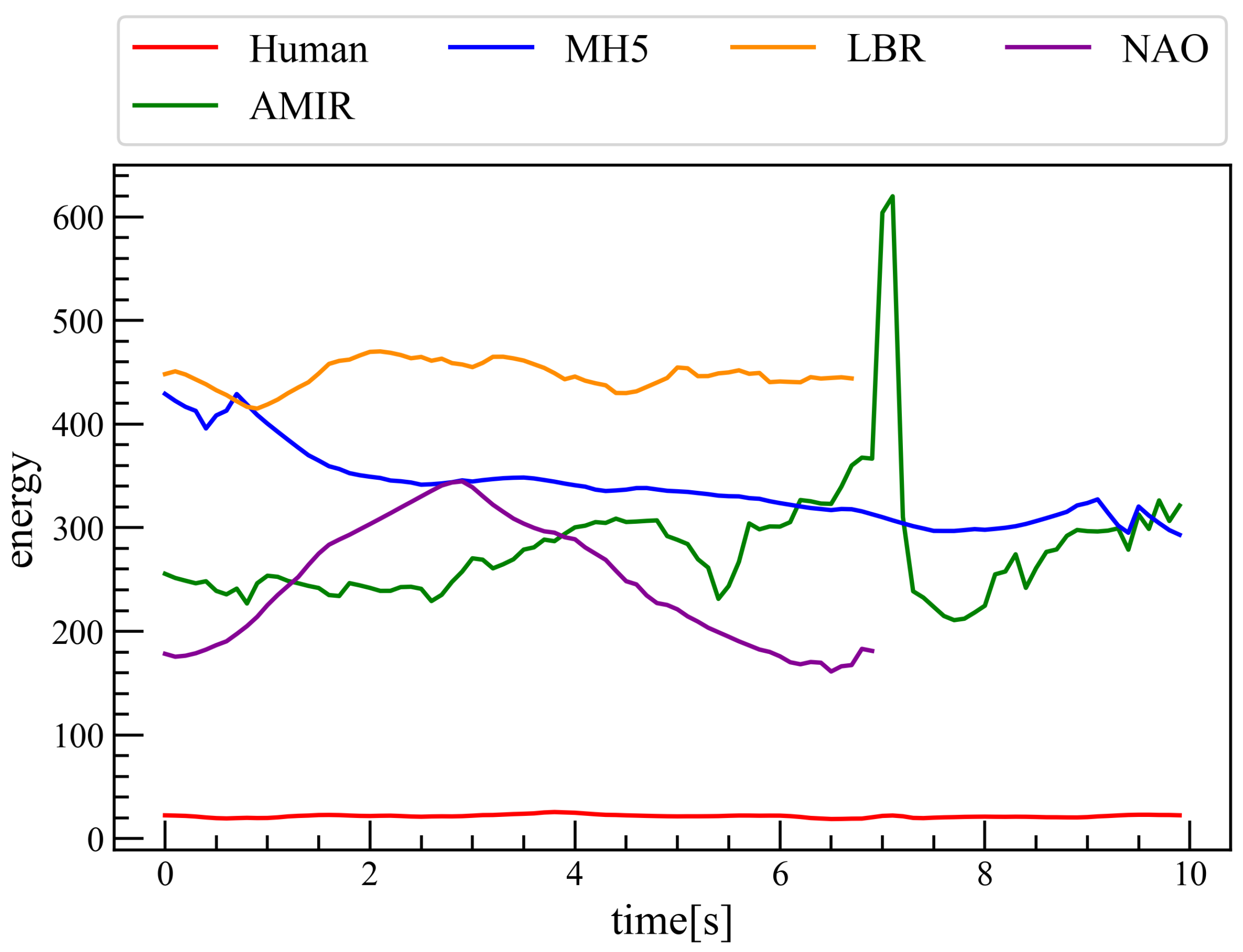
In previous studies on imitation learning across different embodiments, it has been difficult to quantitatively evaluate embodiment gaps in the learned imitation results. Most existing approaches have relied solely on trajectory errors or task success rates, which do not capture how well the robot’s motion preserves the human embodiment characteristics. Figure 20 illustrates the energy differences between the human and the robots after imitation learning.
As shown in Figure 20, NAO exhibits the lowest energy among all robots, indicating the smallest embodiment gap from the human model. In the case of AMIR, the energy remains the second lowest, but a sharp increase occurs around 7 s, consistent with the result observed in Figure 14. This consistency suggests that the IBC model successfully learned and reproduced the motion patterns of the IMK-based teaching data For MH5, the energy remains relatively high up to approximately 8 s but later decreases to a level similar to that of AMIR, implying partial convergence in embodiment similarity. LBR, on the other hand, shows the highest energy throughout the motion, which is likely due to the effect of its kinematic redundancy resulting from seven degrees of freedom.
The energy does not converge to a specific constant value over time. Instead, it represents the instantaneous compatibility between the robot’s reproduced motion and the human demonstration, and is therefore expected to fluctuate during the motion execution. These fluctuations reflect continuous changes in embodiment differences along the trajectory.
The end time of each curve corresponds to the completion of the imitation execution on each robot. Due to differences in the robots’ kinematic capabilities (e.g., workspace limits and motion speed) as well as the output characteristics of the learned imitation models, the duration required to complete the same trajectory varies across platforms.
Because the EBM is trained on human motion, the absolute energy values are not directly comparable across embodiments. Rather, the relative difference between the robot’s energy and the human’s energy serves as a quantitative measure of the embodiment gap after imitation learning. In this sense, convergence is not defined solely by similarity in the range of variation, but rather reflects the embodiment gap, as demonstrated by how closely the robot’s energy trajectory approaches that of a human throughout the entire execution.
Overall, these results confirm that the EBM can capture embodiment gaps even after imitation learning, and that IBC, when trained with IMK-based trajectories, can reproduce not only geometric motion patterns but also embodiment-dependent kinematic tendencies across different robots.

5. Conclusions

In this study, we proposed X-EKBC, an imitation learning framework that enables movement-level imitation on a one-to-one basis between humans and multiple robots with embodiment gaps. To achieve this, the proposed joint angle matrix was utilized to explicitly compare and evaluate the joint structures of humans and robots. By combining it with the Imitation Kinematics framework, it became possible to reconstruct motions that are adapted to each robot’s embodiment while preserving correspondence with the human motion.
In previous imitation learning studies across different embodiments, it has not been possible to quantitatively evaluate embodiment gaps. In this study, by employing an EBM to assess the compatibility between human and robot embodiment models, we were able to quantitatively evaluate the overall motion—including both static differences in joint angles and end-effector poses, as well as dynamic transitions of joint trajectories.
Furthermore, through imitation learning using IBC, motion imitation was successfully achieved for robots with 5, 6, and 7 degrees of freedom, respectively. In addition, by applying the EBM to evaluate the embodiment models of the imitation results, it became possible to perform a comprehensive quantitative assessment of the overall motions obtained from imitation learning across different embodiments an evaluation that had not been achievable in previous studies.
In future work, we aim to extend the proposed framework in several directions. First, we plan to broaden the joint matrix representation by incorporating physical constraints, enabling the modeling of not only kinematic embodiment but also compliance-related characteristics of human joints. Second, although the current imitation learning scheme is formulated as a one-to-one correspondence between a human and a robot, we intend to unify these mappings within a single integrated model. This would reduce teaching cost and improve scalability to multiple embodiments. Finally, the present study focuses primarily on upper-body movements, and expanding the framework to locomotion and whole-body manipulation remains an important challenge for future work.

Author Contributions

Conceptualization, M.T. and K.S.; methodology, M.T.; software, Y.T. and M.T.; validation, Y.T., M.T., and K.S.; formal analysis, Y.T. and M.T.; investigation, Y.T. and M.T.; resources, Y.T.; data curation, Y.T.; writing—original draft preparation, Y.T., M.T., and K.S.; writing—review and editing, Y.T. and K.S.; visualization, Y.T.; supervision, K.S. All authors have read and agreed to the published version of the manuscript.

Funding

This research received no external funding.

Institutional Review Board Statement

Not applicable.

Informed Consent Statement

Verbal informed consent for publication was obtained from all participants. The images included in this manuscript are anonymized (e.g., apply blurring to the face). Because the images do not allow identification of individuals and the use involves minimal risk, written consent was not obtained; participants agreed to the use of the anonymized image data in the submitted manuscript.

Data Availability Statement

The data presented in this study are available on request from the corresponding author.

Conflicts of Interest

The authors declare no conflicts of interest.

References

  1. Argall, B.D.; Chernova, S.; Veloso, M.; Browning, B. A survey of robot learning from demonstration. Robot. Auton. Syst. 2009, 57, 469–483. [Google Scholar] [CrossRef]
  2. Zhang, T.; McCarthy, Z.; Jow, O.; Lee, D.; Chen, X.; Goldberg, K.; Abbeel, P. Deep imitation learning for complex manipulation tasks from virtual reality teleoperation. In Proceedings of the 2018 IEEE International Conference on Robotics and Automation (ICRA), Brisbane, Australia, 21–25 May 2018; pp. 5628–5635. [Google Scholar]
  3. Tykal, M.; Montebelli, A.; Kyrki, V. Incrementally assisted kinesthetic teaching for programming by demonstration. In Proceedings of the 2016 11th ACM/IEEE International Conference on Human-Robot Interaction (HRI), Christchurch, New Zealand, 7–10 March 2016; pp. 205–212. [Google Scholar]
  4. Taylor, M.; Bashkirov, S.; Rico, J.F.; Toriyama, I.; Miyada, N.; Yanagisawa, H.; Ishizuka, K. Learning Bipedal Robot Locomotion from Human Movement. In Proceedings of the 2021 IEEE International Conference on Robotics and Automation (ICRA), Xi’an, China, 30 May–5 June 2021; pp. 2797–2803. [Google Scholar]
  5. Zakka, K.; Zeng, A.; Florence, P.; Tompson, J.; Bohg, J.; Dwibedi, D. Xirl: Cross embodiment inverse reinforcement learning. arXiv 2021, arXiv:2106.03911. [Google Scholar] [CrossRef]
  6. LeCun, Y.; Chopra, S.; Hadsell, R.; Ranzato, M.; Huang, F. A tutorial on energy-based learning. In Predicting Structured Data; Bakir, G., Hofman, T., Scholkopf, B., Smola, A., Taskar, B., Eds.; MIT Press: Cambridge, MA, USA, 2006. [Google Scholar]
  7. Florence, P.; Lynch, C.; Zeng, A.; Ramirez, O.A.; Wahid, A.; Downs, L.; Wong, A.; Lee, J.; Mordatch, I.; Tompson, J. Implicit Behavioral Cloning. In Proceedings of the 5th Conference on Robot Learning, Zurich, Switzerland, 29–31 October 2018; pp. 158–168. [Google Scholar]
  8. Tanaka, M.; Sekiyama, K. Human-Robot Imitation Learning of Movement for Embodiment Gap. In Proceedings of the 2023 IEEE International Conference on Systems, Man, and Cybernetics (SMC), Cybern, MD, USA, 1–4 October 2023; pp. 1733–1738. [Google Scholar]
  9. Tanaka, M.; Sekiyama, K. Human-Robot Imitation Learning for Embodiment Gap. Master’s Thesis, Meijo University, Nagoya, Japan, 2024. [Google Scholar]
  10. Delmerico, J.; Poranne, R.; Bogo, F.; Oleynikova, H.; Vollenweider, E.; Coros, S. Spatial Computing and Intuitive Interaction: Bringing Mixed Reality and Robotics Together. IEEE Robot. Autom. Mag. 2022, 29, 45–57. [Google Scholar] [CrossRef]
  11. Seo, M.; Park, H.A.; Yuan, S.; Zhu, Y.; Sentis, L. LEGATO: Cross-Embodiment Imitation Using a Grasping Tool. IEEE Robot. Autom. Lett. 2025, 10, 2854–2861. [Google Scholar] [CrossRef]
  12. Sharma, P.; Mohan, L.; Pinto, L.; Gupta, A. Multiple interactions made easy (MIME): Large scale demonstrations data for imitation. In Proceedings of the Conference on Robot Learning, Zürich, Switzerland, 29–31 October 2018; pp. 906–915. [Google Scholar]
  13. Yang, L.; Suh, H.J.; Zhao, T.; Graesdal, B.P.; Kelestemur, T.; Wang, J.; Pang, T.; Tedrake, R. Physics-driven data generation for contact-rich manipulation via trajectory optimization. arXiv 2025, arXiv:2502.20382. [Google Scholar]
  14. Wang, Y.; Johns, E. One-Shot Dual-Arm Imitation Learning. arXiv 2025, arXiv:2503.06831. [Google Scholar]
  15. Lum, T.G.W.; Lee, O.Y.; Liu, C.K.; Bohg, J. Crossing the human-robot embodiment gap with sim-to-real rl using one human demonstration. arXiv 2025, arXiv:2504.12609. [Google Scholar]
  16. Dan, P.; Kedia, K.; Chao, A.; Duan, E.W.; Pace, M.A.; Ma, W.C.; Choudhury, S. X-Sim: Cross-Embodiment Learning via Real-to-Sim-to-Real. arXiv 2025, arXiv:2505.07096. [Google Scholar]
  17. Bain, M.; Sommut, C. A Framework for Behavioral Cloning. Mach. Intell. 1999, 15, 103–129. [Google Scholar]
  18. Finn, C.; Levine, S.; Abbeel, P. Guided Cost Learning: Deep Inverse OptimalControl via Policy Optimization. In Proceedings of the 33rd International Conference on Machine Learning, New York, NY, USA, 20–22 June 2016; pp. 49–58. [Google Scholar]
  19. Ho, J.; Ermon, S. Generative adversarial imitation learning. arXiv 2016, arXiv:1606.03476. [Google Scholar] [CrossRef]
  20. Zhao, T.Z.; Kumar, V.; Levine, S.; Finn, C. Learning fine-grained bimanual manipulation with low-cost hardware. arXiv 2023, arXiv:2304.13705. [Google Scholar]
  21. Franzmeyer, T.; Torr, P.; Henriques, J.F. Learn what matters: Crossdomain imitation learning with task-relevant embeddings. arXiv 2022, arXiv:2209.12093. [Google Scholar]
  22. Fickinger, A.; Cohen, S.; Russell, S.; Amos, B. Cross-domain imitation learning via optimal transport. arXiv 2021, arXiv:2110.03684. [Google Scholar]
  23. Sermanet, P.; Lynch, C.; Hsu, J.; Levine, S. Time-Contrastive Networks: SelfSupervised Learning from Multi-view Observation. In Proceedings of the 2017 IEEE Conference on Computer Vision and Pattern Recognition Workshops (CVPRW), Honolulu, HI, USA, 21–26 July 2017; pp. 486–487. [Google Scholar]
  24. Xu, M.; Xu, Z.; Chi, C.; Veloso, M.; Song, S. Xskill: Cross embodiment skill discovery. In Proceedings of the Conference on Robot Learning (CoRL), Atlanta, GA, USA, 6–9 November 2023; pp. 3536–3555. [Google Scholar]
  25. Kim, H.; Kang, J.; Kang, H.; Cho, M.; Kim, S.J.; Lee, Y. UniSkill: Imitating Human Videos via Cross-Embodiment Skill Representations. arXiv 2025, arXiv:2505.08787. [Google Scholar]
  26. Pauly, L.; Agboh, W.C.; Hogg, D.C.; Fuentes, R. O2a: One-shot observational learning with action vectors. Front. Robot. AI 2021, 8, 686368. [Google Scholar] [CrossRef]
  27. O’Neill, A.; Rehman, A.; Gupta, A.; Maddukuri, A.; Gupta, A.; Padalkar, A.; Lee, A.; Pooley, A.; Gupta, A.; Mandlekar, A.; et al. Open X-Embodiment: Robotic Learning Datasets and RT-X Models. arXiv 2024, arXiv:2310.08864. [Google Scholar]
  28. Torabi, F.; Warnell, G.; Stone, P. Behavioral Cloning from Observation. In Proceedings of the Twenty-Seventh International Joint Conference on Artificial Intelligencem, Stockholm, Sweden, 13–19 July 2018; pp. 4950–4957. [Google Scholar]
  29. Torabi, F.; Warnell, G.; Stone, P. Generative adversarial imitation from observation. arXiv 2018, arXiv:1807.06158. [Google Scholar]
  30. Pavse, B.S.; Torabi, F.; Hanna, J.; Warnell, G.; Stone, P. RIDM: Reinforced Inverse Dynamics Modeling for Learning from a Single Observed Demonstration. IEEE Robot. Autom. Lett. 2020, 5, 6262–6269. [Google Scholar] [CrossRef]
  31. Torabi, F.; Warnell, G.; Stone, P. DEALIO: Data-Efficient Adversarial Learning for Imitation from Observation. In Proceedings of the 2021 IEEE/RSJ International Conference on Intelligent Robots and Systems (IROS), Prague, Czech Republic, 27 September–1 October 2021; pp. 2391–2397. [Google Scholar]
  32. Hudson, E.; Warnell, G.; Torabi, F.; Stone, P. Skeletal Feature Compensation for Imitation Learning with Embodiment Mismatch. In Proceedings of the 2022 International Conference on Robotics and Automation (ICRA), Philadelphia, PA, USA, 23–27 May 2022; pp. 2482–2488. [Google Scholar]
  33. Hiruma, H.; Ito, H.; Mori, H.; Ogata, T. Deep Active Visual Attention for Real-Time Robot Motion Generation: Emergence of Tool-Body Assimilation and Adaptive Tool-Use. IEEE Robot. Autom. Lett. 2022, 7, 8550–8557. [Google Scholar] [CrossRef]
  34. Sugihara, T. Solvability-Unconcerned Inverse Kinematics by the Levenberg-Marquardt Method. IEEE Trans. Robot. 2011, 27, 984–991. [Google Scholar] [CrossRef]
  35. Cao, Z.; Martinez, G.H.; Simon, T.; Wei, S.E.; Sheikh, Y. OpenPose: Realtime Multi-Person 2D Pose Estimation using Part Affinity Fields. IEEE Trans. Pattern Anal. Mach. Intell. 2021, 43, 172–186. [Google Scholar] [CrossRef]
  36. Kingma, D.P.; Ba, J. Adam: A method for stochastic optimization. arXiv 2014, arXiv:1412.6980. [Google Scholar]
  37. Tola, D.; Corke, P. Understanding urdf: A dataset and analysis. IEEE Robot. Autom. Lett. 2024, 9, 4479–4486. [Google Scholar] [CrossRef]
  38. Busy, M.; Caniot, M. qiBullet, a Bullet-based simulator for the Pepper and NAO robots. arXiv 2019, arXiv:1909.00779. [Google Scholar]
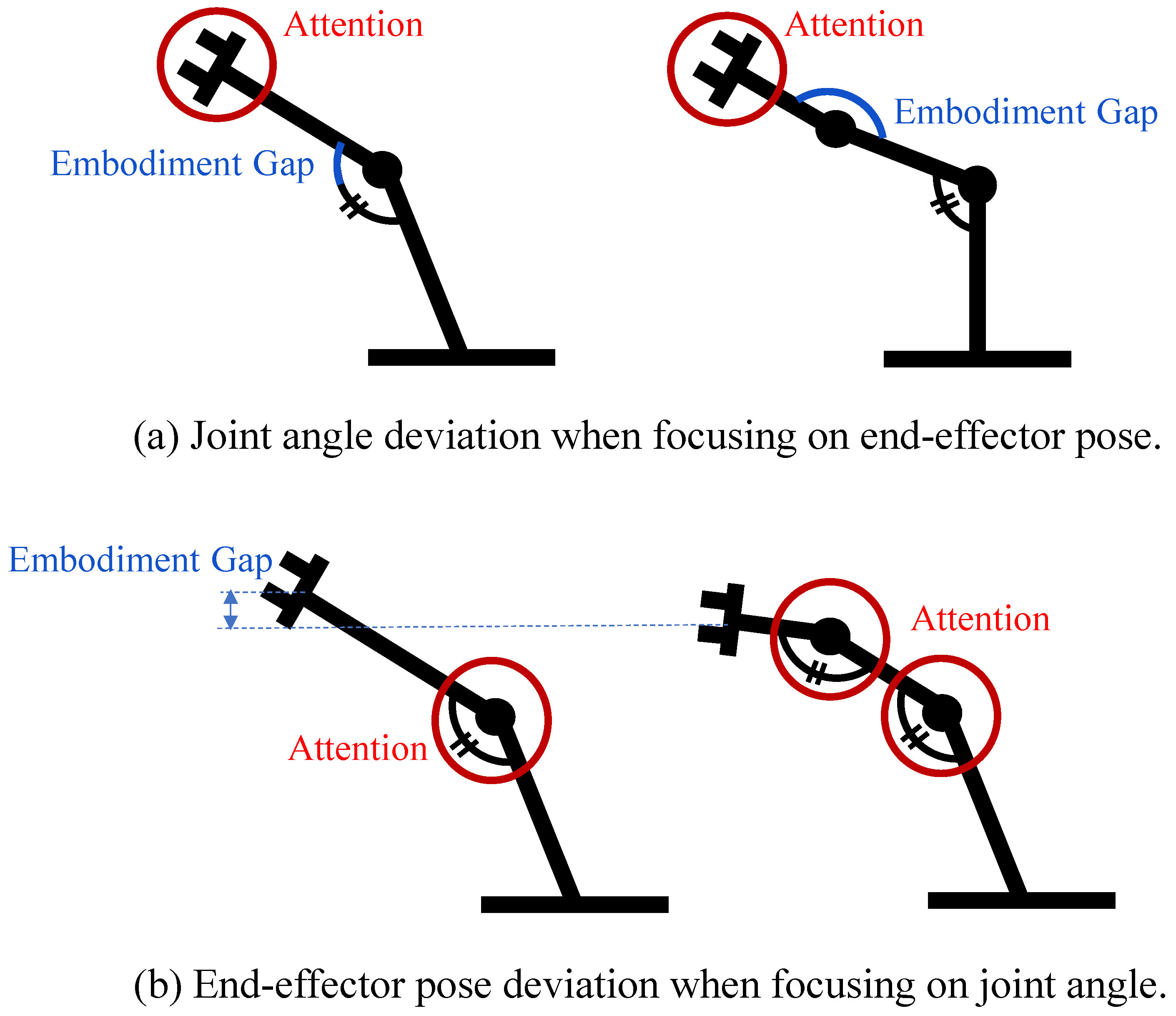
Figure 1. Trade-off between end-effector pose and joint angles due to the embodiment gap.
Machines 13 01134 g001
Figure 2. Architecture of Cross-Embodiment Kinematic Behavioral Cloning (X-EKBC).
Machines 13 01134 g002
Figure 3. The human pose estimation obtained using OpenPose.
Machines 13 01134 g003
Figure 4. Definitions for constructing joint matrices.
Machines 13 01134 g004
Figure 5. Construction process of joint matrices in the human arm.
Machines 13 01134 g005
Figure 6. Construction process of joint matrices in the robot arm (5 DoFs).
Machines 13 01134 g006
Figure 7. Construction process of joint matrices in the robot arm (7 DoFs).
Machines 13 01134 g007
Figure 8. Learning embodiment models with EBM.
Machines 13 01134 g008
Figure 9. Structure of embodiment model inputs for multiple robots using the flattened joint matrix representation.
Machines 13 01134 g009
Figure 10. Leaining imitation model with EBM.
Machines 13 01134 g010
Figure 11. Configuration of the human and robot joints.
Machines 13 01134 g011
Figure 12. Comparison of human and reconstructed robot motion end-effector trajectories. Red is human’s end-effector position. Blue is reconstructed robot’s end-effector position by IK. Black is robot’s end-effector position that directly transfers the human joint angles to the robot. Green is reconstructed robot’s end-effector position by IMK.
Machines 13 01134 g012
Figure 13. Comparison of human and reconstructed robot motion joint angle transitions. Red: human angles, Green: AMIR angles, Purple: NAO angles, Blue: MH5 angles, Orange: LBR angles.
Machines 13 01134 g013
Figure 14. Comparison of embodiment gaps for energy.
Machines 13 01134 g014
Figure 15. Comparison of energy from ablation of joint angles.
Machines 13 01134 g015
Figure 16. Comparison of energy from ablation of end-effector pose.
Machines 13 01134 g016
Figure 17. Comparison of energy from ablation of anjoint angular velocitiesgle.
Machines 13 01134 g017
Figure 18. Robot end-effector trajectory with imitation learning.
Machines 13 01134 g018
Figure 19. The Behavior of the robot obtained through imitation learning at times (i) to (iv).
Machines 13 01134 g019
Figure 20. Embodiment gaps evaluated by the embodiment model after imitation learning.
Machines 13 01134 g020
Table 1. Definition of joint matrix K .
SymbolDefinitionDescription
ijoint set order-
jrotation axis1: Roll 2: Pitch 3: Yaw
k i j joint order0: No joint
Disclaimer/Publisher’s Note: The statements, opinions and data contained in all publications are solely those of the individual author(s) and contributor(s) and not of MDPI and/or the editor(s). MDPI and/or the editor(s) disclaim responsibility for any injury to people or property resulting from any ideas, methods, instructions or products referred to in the content.