Abstract
Current research on tower crane control lacks high-fidelity models and fails to account for the coupling effects between the tower crane structure and the hoisting and luffing systems. A new dynamic analysis platform based on the flexible multibody system theory is proposed in this investigation for the tower crane which contains a large-scale steel structure and hoisting mechanisms undergoing large displacements and large deformations. The Arbitrary Lagrangian–Eulerian–Absolute Nodal Coordinate Formulation (ALE–ANCF) cable element was employed to model the varying length of the steel rope in the hoisting mechanisms. Nonlinear kinetic equations were used to describe the motion of a luffing trolley. The solving strategy of the system’s dynamical equations are presented. Two different trajectories were tested. Simulation results demonstrate the feasibility and rationality of the proposed dynamic analysis platform. The primary conclusion is that this platform serves as a reliable and high-fidelity testbed for developing and evaluating advanced control algorithms under realistic dynamic conditions, thereby providing a dependable tool for both research and engineering applications.
1. Introduction
Tower cranes have always played an irreplaceable role in construction engineering. The practical need for suppressing crane swing, along with the trend towards unmanned and intelligent operation, demands accurate dynamic analysis and control. The tower crane system includes jib structure, hoisting, and the luffing mechanism. When the slewing motion of the tower crane is not considered, the structural dynamics of the tower crane can be characterized as a small deformation problem. However, the hoisting and luffing mechanisms may undergo motions involving large displacements and deformations. The dynamic properties of these subsystems are fundamentally different, yet they are integrated through highly nonlinear kinematic constraints into a complex, large-scale multi-flexible-body system. Consequently, its dynamic modeling and analysis persist as a challenging problem [1,2,3]. Vaughan et al. conducted control research on the double-pendulum model of tower cranes [4]. While this model captures basic payload swing characteristics, it oversimplifies the actual system by ignoring the structural flexibility of the jib and hoisting rope, limiting its applicability in high-precision control scenarios. Duong et al. proposed a hybrid evolutionary algorithm that integrates constriction particle swarm optimization with genetic algorithm operators utilizing binary encoding for the control study of an underactuated three-dimensional tower crane [5]. Le et al. designed a robust nonlinear controller for the complex working conditions of a tower crane, considering both trolley translation and tower rotation [6]. Although the controller accounts for multiple motion states, it fails to address parametric uncertainties caused by structural deformation, leading to a potential control performance degradation in complex environments. Boeck and Kugi developed and applied a path-following controller to a laboratory tower crane [7]. Chen et al. proposed an adaptive tracking control method to address the parametric uncertainties in tower crane systems [8]. Zhang et al. established a dynamic model of tower cranes considering the double-pendulum and spherical-pendulum effects [9]. Meanwhile, they also established dynamic models of a tower crane with different cable lengths and, based on this foundation, proposed an adaptive anti-sway control method [10]. These models enhance the accuracy of dynamic description, but the control method does not fully integrate the flexible characteristics of the boom, leading to suboptimal anti-sway performance under large-load conditions. Ouyang et al. designed a nonlinear adaptive tracking controller for double-pendulum tower cranes. Additionally, they proposed an adaptive integral sliding mode control method for 4-DOF tower crane systems [11,12]. Ramli et al. conducted an extensive review of control schemes for various types of crane systems since the 21st century [13]. Conventional control strategies for suppressing tower crane payload swing are typically developed under the rigid-body assumption, neglecting structural deformation. However, recent studies are increasingly addressing the influence of structural flexibility on control performance [14,15].
Reviewing existing research reveals that dynamic models employed for tower crane control are frequently subject to significant simplification. Moreover, the evaluation of control strategies is typically performed using these simplified models. The author contends that verification of any control strategy, irrespective of its foundational model, ought to be undertaken within a high-fidelity dynamic simulation environment that accurately mirrors a real-world tower crane with comprehensive detail. A pivotal challenge in achieving this is the accurate modeling of the hoisting rope—a component notable for its substantial flexibility in the hoisting-luffing system. As an important theoretical tool in the analysis of multibody system dynamics, the Absolute Nodal Coordinate Formulation (ANCF) is particularly well-suited for describing the dynamic behaviors of flexible bodies undergoing large displacements and large deformations. Gerstmayr and Irschik validated the beam and plate formulations proposed within the ANCF framework through numerical examples of a cantilever beam undergoing large deformations [16]. Wang et al. established a simulation method, based on the ANCF curved beam element, for capturing the frictional contact dynamics in large-scale continuous contact drives involving thin beams subject to large deformations and overall global motion [17,18]. This method effectively handles contact problems, but it is not tailored to the time-varying length characteristics of tower crane hoisting ropes. Although large deformations are not typically encountered in railway vehicle dynamics, the ANCF can also be employed for railway vehicle simulation, specifically for modeling track geometry and pantograph/catenary interactions [19,20]. Utilizing gradient deficient beam elements of ANCF, Luo et al. developed a mechanical model for the space elevator system. This model is capable of accurately describing the flexible dynamics exhibited by the rope in a space elevator [21]. Zhang et al. proposed a reformulation for the axial strain in flexible cables via the construction of an equivalent rod element. This work led to the derivation of a strain-decoupled ANCF cable element and the establishment of a decoupled model for stranded cables [22]. Peng et al. proposed a novel method based on adaptive variable-length cable elements within the ANCF to accurately compute the initial equilibrium configuration of railway catenaries [23]. The method addresses variable-length cable modeling, but it does not account for the nonlinear kinematic constraints between the cable and other tower crane components. Zhang et al. enhanced the computational efficiency of the ANCF cable element by streamlining the formulation of the generalized elastic force and the tangent stiffness matrix, which is expressed in a dot product form based on curvature [24]. Wang et al. presents an adaptive ANCF described by the Arbitrary Lagrangian–Eulerian (ALE) formulation, for the purpose of studying the nonlinear dynamic behavior of underwater tethered systems with varying lengths as they traverse obstacles [25]. Yang et al. employed the Absolute Nodal Coordinate Formulation with Arbitrary Lagrangian–Eulerian description to model a variable-length flexible towing cables and validated the accuracy of the modeling approach using a variable-length pendulum, towing cable, and cable in waves [26]. Escalona and Mohammadi introduced two new advancements in the Arbitrary Lagrangian–Eulerian Modal Method for modeling the dynamics of reeving systems. The first concerns the dynamic modeling of sheaves. By introducing the sheaves’ rotation angle as a generalized coordinate and formulating the no-slip assumption as a linear constraint equation, precise torque balance at the sheaves is ensured. This approach avoids nonlinear kinematic constraints and simultaneously reveals the influence of the sheaves’ rotational inertia on the system dynamics. The second advancement addresses the issue of non-constant axial force in long cable span systems. It introduces axial modal coordinates to simulate the linearly varying axial force along the element. Numerical results indicate that just three modal coordinates are sufficient to effectively capture this variation. These enhancements improve the simulation accuracy for the dynamic behavior of complex systems [27]. Shabana discussed potential future research directions for applying ANCF finite elements in emerging fields such as soft tissues and materials, which are relevant to the broader computational engineering and scientific community [28]. Li et al. proposed a payload swing control method incorporating phase plane analysis while accounting for tower crane vibrations; however, the model used in their study still relies on a simplified beam formulation and does not consider the real-time deformation of the crane boom [29].
A review of the aforementioned research readily reveals that the hoisting and luffing system wire rope models for tower cranes, based on the ANCF, have not yet been effectively integrated with the tower body and jib structure to form a usable flexible multibody system dynamics simulation platform. The tower crane’s trolley moves along a jib that undergoes deformation, while the hoisting rope changes its length in real time, forming a characteristic time varying topology. To address these features, this paper will employ multibody system dynamics and the ANCF as the theoretical foundation, utilize cable elements based on the ALE description as the modeling tool, and introduce nonlinear kinematic constraint equations. The objective of this approach is to realize the effective integration of a complete tower crane model. The resulting integrated platform is designed to serve as a reliable and efficient testbed for validating diverse control algorithms pertaining to tower cranes, which contributes to substantial savings in experimental costs and development time. The key innovation of this research is the creation of a dedicated simulation platform that facilitates the testing of various control algorithms, effectively filling a critical gap identified in current research endeavors.
The rest of this paper is organized as follows. Section 2 presents the modeling of the hoisting wire rope, including the kinematic description of the ALE-ANCF element and the elastic force model of the element. In Section 3, the establishment of the dynamic model for the tower crane’s hoisting rope and flexible multibody model for the tower crane system is introduced. Section 4 demonstrates the process of dynamic solution. In Section 5, author conducts the simulation and verification of numerical examples. Finally, the work of this paper is summarized in Section 6.
2. Modeling of Hoisting Wire Rope
2.1. Element Kinematic Description
During the hoisting process of a tower crane, the length of the wire rope will vary according to the hoisting trajectory. This article establishes a variable length hoisting wire rope model based on ALE-ANCF cable element. As illustrated in Figure 1, the model extends the conventional ANCF cable element by incorporating two material coordinates to specify the element length. Each ALE-ANCF element comprises two nodes, with each node characterized by seven nodal coordinates. The configuration of the ALE-ANCF cable element is described by the global position vectors, gradient vectors, and material coordinates.
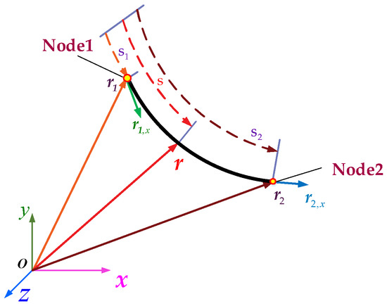
Figure 1.
14 degree-of-freedom ALE-ANCF cable element.
The ALE-ANCF cable element is mathematically represented by the following vector:
here, denotes vector of ALE-ANCF cable element, and represents time. The global position vectors , and gradient vectors , of two nodes are taken as nodal coordinates. , represent the material coordinates associated with each node. In a three-dimensional space, each node contributes three translational degrees of freedom from its position vector and three rotational degrees of freedom from its gradient vector, along with the material coordinate, resulting in a total of 14 degrees of freedom per element.
The global position vector r of an arbitrary point in the element is formulated through the interpolation r = Se, a relation in which e represents the nodal coordinate vector and S signifies the shape function matrix. This matrix is expressed as follows:
The components of the shape function matrix are defined as follows:
In the equation, represents the dimensionless material coordinate. l denotes the element length defined by the material coordinates of the nodal coordinate and .
The velocity and acceleration of any point inside the element are derived by computing the first and second temporal derivatives of r = Se:
is shape function matrix associated with velocity:
is the quadratic term of velocity:
The consistent mass matrix of the element is formulated as:
A significant feature of the ANCF description is that the mass matrix remains constant. This property allows for the decomposition of the mass matrix during the pre-processing phase, thereby enhancing computational efficiency in dynamic simulations.
2.2. Element Elastic Model
An enhanced cable elastic force model, originally proposed by Gerstmayr and Irschik, is implemented for the ALE-ANCF cable element. The strain energy of the element accounts for both axial stretching and bending curvature:
where l represents the undeformed length of the ALE-ANCF cable element, E is the modulus of elasticity, A is the area of cross-section and I is the second moment of the cross-section. The axial strain is defined as:
The curvature K, representing the spatial bending measure, is given by:
and are the first and second derivative with respect to the material coordinates, respectively. The ALE-ANCF approach decouples the motion of the computational mesh from the material points. Consequently, these derivatives are redefined in terms of the isoparametric coordinate :
where is the dimensionless material coordinate, and are the first and second derivatives of the shape function matrix derivatives with respect to .
The generalized elastic force vector is obtained by differentiating the strain energy with respect to the nodal coordinate vector:
The partial derivative of the axial strain with respect to the i-th nodal coordinate component is:
where is the i-th column of the shape function derivative matrix . The derivative of the curvature K is expressed as a quotient:
with the derivatives of the numerator and denominator being:
signifies the i-th column of the second derivative of the shape function.
For the numerical solution of the system’s equations of motion, implicit integrators are often employed due to their ability to handle larger time steps. These methods require solving nonlinear algebraic equations at each step, typically via the Newton–Raphson iteration, which necessitates the Jacobian matrix of the elastic forces. This Jacobian is equivalent to the second partial derivatives of the strain energy:
In this equation, the second derivative of the axial strain is:
The second derivative of the curvature involves more complex terms derived from the quotient rule:
where the second derivatives of f and g are:
Notably, the items , , and , depend solely on the material coordinates and element dimensions. Their independence from the current configuration allows for precomputation during the preprocessing stage, thereby enhancing overall computational efficiency.
3. Modeling of Tower Crane System
3.1. Dynamic Modeling of Hoisting Rope of Tower Crane
A simplified finite element model of the tower crane was developed for this research, incorporating the tower body, jib, counter weight arm, and the hoisting rope. The deformation behavior of the tower–jib structure was captured using linear finite-strain beam elements governed by the Timoshenko beam theory. Concurrently, the model for the hoisting rope was constructed employing the ALE-ANCF.
The hoisting rope in the lifting system can be subdivided into multiple ALE-ANCF cable elements. To improve the computational efficiency of the system’s dynamic equations, as shown in Figure 2, the modeling of the hoisting rope is categorized into ALE-ANCF cable elements with fixed length and those with variable length.
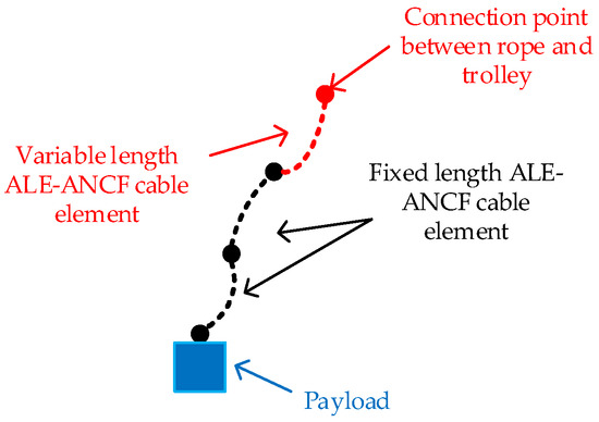
Figure 2.
The hoisting rope model established by ALE-ANCF cable element.
The information of the variable length cable elements requires real-time updates, while the nodal information of the fixed length elements remains unchanged. This approach ensures that the total number of elements for the entire hoisting rope remains minimized when the cable length changes, and the number of elements requiring real-time information updates is kept to a minimum, thereby enhancing computational efficiency. The dynamic equations for the hoisting rope are established as follows:
where is the mass matrix of the hoisting rope element, is the vector of additional generalized inertial force:
is the vector of generalized external force:
During the hoisting process, the length of the hoisting rope changes in real time according to the transportation trajectory, resulting in a varying mass matrix that requires real-time updates during solution. As mentioned earlier, to accurately describe the state of the hoisting rope while balancing computational efficiency and precision in dynamic analysis, the rope elements can be divided into fixed-length and variable-length elements. Consequently, the number of ALE-ANCF elements used in modeling the hoisting rope needs to be adjusted dynamically.
This research adopts an adaptive meshing strategy [25], a standard element length is set. If a variable-length element exceeds the maximum length of 1.5 , it is split into one variable length element and one fixed length element to prevent a decline in solution accuracy due to excessively long elements. If its length falls below the minimum length of 0.5 , it is merged with an adjacent fixed length element to form a new variable length element. If the length remains between the minimum and maximum thresholds, the variable-length element is retained unchanged. It is noteworthy that researchers must select appropriate threshold value to prevent the boundary elements from becoming excessively coarse or fine, as improper sizing may lead to a degradation in discretization accuracy and matrix singularity, ultimately causing simulation failure [30]. Additionally, although dynamic remeshing might introduce disturbances (such as energy catastrophe under drastic topological changes), reasonable threshold value can effectively suppress numerical oscillations.
3.2. Assembly of Tower Crane System Model Based on Motion Constraints
In this section, the beam element in the traditional Finite Element Method (FEM) is used to describe the structure of the tower crane. To describe the luffing motion of the tower crane, a non-generalized coordinate needs to be introduced to define the position of the trolley on the jib. Through kinematic constraints, the hoisting rope is connected to the tower crane. It is assumed that the position of the trolley is , and the position of the wire rope’s endpoint is . These two positions coincide in space. The schematic view of the constraints between the tower crane and hoisting rope is given in Figure 3. The constraint equations are:
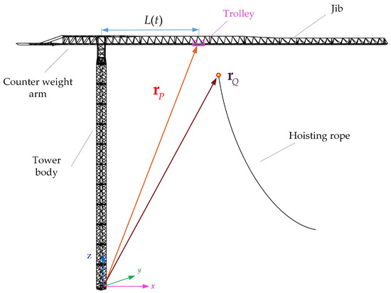
Figure 3.
Constraints between the tower crane and hoisting rope.
Thus, the multibody system dynamic equations of the tower crane are:
where is the mass matrix of tower crane, and are generalized coordinates of tower crane and hoisting rope, respectively. is the generalized elastic force vector of the whole system, is the vector of additional generalized inertial force of hoisting rope, represents the generalized external force vector, is the Lagrange multiplier, is the Jacobian e matrix of constraint equations with respect to generalized coordinate, represents system constraint equations.
As shown in Figure 4, the position of the trolley is determined by interpolation from the beam element it is on:
where is the length of the beam element, and are the node coordinates of endpoints A and B of the beam element, due to structural deformation, the nodal coordinates of beam element vary with time.
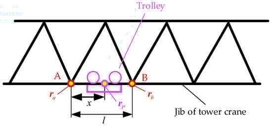
Figure 4.
Schematic diagram of trolley position calculation.
4. Solution Methods for the Complete System Dynamic Equations
As illustrated in Figure 5, the multibody dynamic equations of the tower crane are solved using NewMark solver. In this model, the steel structure is modeled via the conventional finite element method, with its mass and stiffness matrices remaining constant. The hoisting rope section changes its length according to the transportation trajectory. Consequently, its corresponding mass matrix , elastic force vector , generalized additional inertial force vector , system constraint equations , Jacobian matrix of the system constraint equations with respect to the nodal coordinates , Lagrange multiplier vector , and generalized external force vector all require updating during the solution process. Since the trolley’s trajectory is calculated based on linear interpolation of the tower crane jib’s positional coordinates, when the crane is activated and responds, causing the jib’s positional coordinates to change, it becomes necessary to synchronously update these jib coordinates during the solution process to achieve control of the hoisting trajectory under the condition of structural deformation of the tower crane.
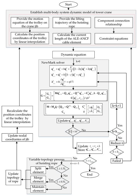
Figure 5.
Flowchart of dynamic solution.
5. Numerical Simulation and Validation
This study used a T8063 flat-top tower crane (Zhejiang Huba Construction Machinery Co., Ltd., Haining, China) from a certain brand as an example to carry out virtual prototype simulation validation. This model crane has a maximum lifting height of 66 m, a rated load moment of 4100 kN·m, a maximum lifting capacity of 125 kN, and a maximum working radius of 80 m. At this maximum radius, its maximum lifting capacity is 36 kN. The combined self-weight of the trolley and hook is 30.44 kN. The counter weight of the tower crane is 100 kN, with a moment jib of 22 m. The tower crane model comprises 701 nodes and 1500 elements. In this case study, the tower structure undergoes reduced-order modeling, retaining the first 100 modes. The initial position of the trolley is at 14 m along the jib, with a travel speed of 1 m/s horizontally to the right. The hoisting rope is discretized into 61 nodes and 60 elements. The remaining relevant parameters of the tower crane and the hoisting rope are provided in Table 1 and Table 2, respectively.

Table 1.
Parameters of the tower crane.
Table 2.
Parameters of the hoisting rope.
As shown in Figure 6, in order to simulate the realistic hoisting trajectory of the tower crane, two types of envelope trajectories in the XOZ plane were generated by configuring different obstacle arrangements. The Root Mean Square Error (RMSE), which is calculated as the square root of the average of squared positional errors between a set of comparison points on the actual and ideal trajectories. The formulation is given in Equation (27). According to calculations, the RMS error for the straight and curved trajectories shown in Figure 7 are 0.4255 m and 0.4765 m, respectively. The usability of the proposed tower crane testing platform is verified.
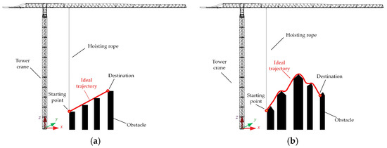
Figure 6.
Tower crane system under different trajectories. (a) Tower crane system under straight trajectory. (b) Tower crane system under curve trajectory.
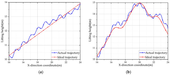
Figure 7.
Lifting height of the payload under different trajectories. (a) Lifting height of the payload under straight trajectory. (b) Lifting height of the payload under curve trajectory.
To accurately simulate the hoisting process where the rope length dynamically adapts to a predefined trajectory, a dynamic mesh refinement strategy is employed. This approach automatically increases the spatial discretization (nodes and elements) during rope extension and coarsens it during contraction, ensuring solution accuracy and computational efficiency.
Figure 8 illustrates the process of subdividing the ALE-ANCF cable element into a varying number of segments based on its length. In the straight trajectory, the payload is lifted upward, and the length of the hoisting rope continuously shortens, resulting in a corresponding reduction in the number of nodes and elements in the associated model. As the payload descends along the curved trajectory, the hoisting rope elongates, so too does the number of nodes and elements in the corresponding model increase. This demonstrates that the variation in the number of cable elements and nodes aligns with the proposed control law.
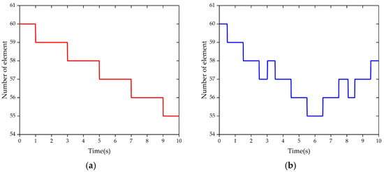
Figure 8.
The numbers of ALE-ANCF cable element under different trajectories. (a) The numbers of cable element under straight trajectory. (b) The numbers of cable element under curve trajectory.
Figure 9 demonstrates the horizontal movement of the driver’s room during operation along two different hoisting trajectories. The vertical deformation of jib free tip during the hoisting operation is illustrated in Figure 10. The comparative results demonstrate that the proposed modeling method in this study effectively achieves various hoisting trajectories while accounting for the deformation of the tower crane jib. The “effectiveness” demonstrated here refers to the platform’s capability to produce physically plausible results for subsequent analysis, while a full validation of accuracy against physical data remains a subject for future case-specific studies.
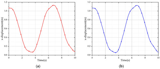
Figure 9.
x displacement of the driver’s room under different trajectories. (a) x displacement of the driver’s room under straight trajectory. (b) x displacement of the driver’s room under curve trajectory.
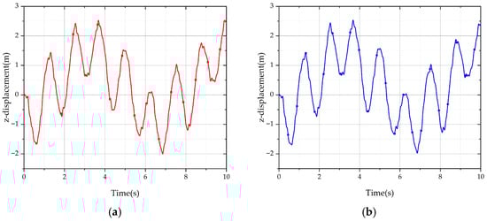
Figure 10.
z displacement of jib free tip under different trajectories. (a) z displacement of jib free tip under straight trajectory. (b) z displacement of end of jib under curve trajectory.
The motion sequence of the hoisting rope along different trajectories at various time points are illustrated in Figure 11 and Figure 12. The figure also shows the displacement deformation of the tower crane structure along the z-direction. The simulation platform developed by the author effectively demonstrates the real-time deformation of the jib induced by the payload’s amplitude variation during tower crane operation. Figure 13 presents overall and local views of the tower crane at its jib tip’s peak displacement, showing the von Mises stress distribution. The maximum stress is within the material’s allowable limit.
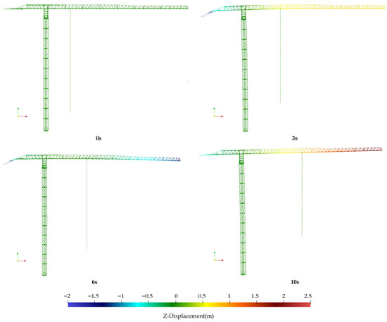
Figure 11.
Configuration of tower system under straight trajectory at different time.
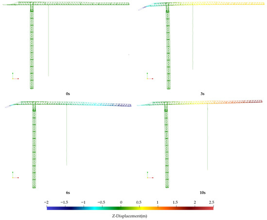
Figure 12.
Configuration of tower system under curve trajectory at different time.
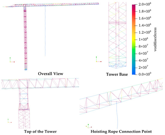
Figure 13.
Stress diagram of the tower crane at its jib tip’s peak displacement.
6. Conclusions
A new flexible multibody system dynamic analysis platform for the tower crane is proposed in this investigation. The tower crane system model contains the steel structure which is discretized based on traditional finite element theory and the hoisting mechanism which is modeled the ALE-ANCF cable element. It can accurately reproduce the process of hoisting, reeling in, and unwinding the steel wire rope in the hoisting mechanism. The motion of the luffing trolley is described through the nonlinear kinematic constraint equation. The actually spatial position of the trolley is determined by the projection of the jib element topology. The solving strategy of the system dynamic equation is proposed based on the NewMark method. In order to test the feasibility and rationality of the proposed tower crane dynamic analysis platform, two different trajectory planning for the lifted load in the lifting plane were simulated. The RMS errors for the two trajectories were 0.4255 m and 0.4725 m, respectively. These served as error references for the performance evaluation of control strategies put forward by future researchers. The dynamic response of the tower crane structure, the position of the trolley, and the configuration of the hoisting rope can be obtained. The primary contribution of this study lies in the establishment of a simulation testbed. This study provides a platform for examining the effectiveness of anti-swing strategies and control methods for tower cranes. Numerical results show that the proposed modeling and simulation methodology constitutes a reliable tool for testing the trajectory planning or command smoothing strategies in engineering applications. Extending the platform to include slewing motion, which may introduce out-of-plane forces and gyroscopic effects, is identified as a critical objective for future research.
Author Contributions
Conceptualization, Z.Y.; methodology, Z.Y.; software, H.L.; validation, Z.Y.; formal analysis, H.L.; investigation, H.L.; resources, Z.Y. and H.L.; data curation, H.L.; writing, H.L.; visualization, H.L.; supervision, Z.Y.; project administration, Z.Y. All authors have read and agreed to the published version of the manuscript.
Funding
This research was funded by the Open Research Fund of the State Key Laboratory of Western Green Building, grant number LSKF202327.
Data Availability Statement
Data are contained within the article.
Conflicts of Interest
The authors declare no conflicts of interest.
Nomenclature
| , , | the nodal coordinate vector of element, tower crane, hoisting rope |
| the time | |
| , | the global position and gradient vector of node |
| the material coordinate of node | |
| , , | the global position, velocity, acceleration of an arbitrary point in the element |
| the shape function of element | |
| , , , | the components of the shape function |
| the dimensionless material coordinate | |
| the length of element | |
| the material coordinate of an arbitrary point in the element | |
| , , , | the velocity, acceleration of material coordinates of node 1, 2 |
| the quadratic term of velocity | |
| the shape function matrix associated with velocity | |
| the first derivative of shape function with respect to time | |
| the generalized velocity of element nodal coordinate | |
| , , | the generalized acceleration of element nodal coordinate |
| , , | the mass matrix of element, tower crane, hoisting rope |
| the identity matrix | |
| the strain energy | |
| the cross-section area of element | |
| the modulus of elasticity | |
| the second moment of the cross-section | |
| the strain along the axis | |
| the spatial measurement of curvature | |
| , | the first and second derivative with respect to the material coordinates |
| , | the first and second derivative of the shape function matrix with respect to the isoparametric coordinate |
| the i,j-th components of nodal coordinate vector | |
| the i-th row and j-th column components of Jacobian matrix in the element elastic force | |
| , , | the generalized elastic force of element, hoisting rope, entire system |
| , | the i-th column of the first and second derivative of element shape function with respect to the material coordinate |
| the integrated functions in the formulation of the Jacobian matrix of the element elastic force | |
| the additional generalized inertial force of hoisting rope | |
| , | the generalized external force of hoisting rope, entire system |
| the Lagrange multiplier | |
| the system constraint equations | |
| the Jacobian matrix of constraint equation with respect to generalized coordinates | |
| the external force | |
| the reference density | |
| , | the position of the trolley, wire rope’s endpoint |
| the motion equation of the trolley | |
| the standard element length | |
| , | the nodal coordinates at both ends of the beam element |
References
- Ju, F.; Choo, Y.S. Dynamic Analysis of Tower Cranes. J. Eng. Mech. 2005, 131, 88–96. [Google Scholar] [CrossRef]
- Ju, F.; Choo, Y.S.; Cui, F.S. Dynamic response of tower crane induced by the pendulum motion of the payload. Int. J. Solids Struct. 2006, 43, 376–389. [Google Scholar] [CrossRef]
- Yang, W.; Zhang, Z.; Shen, R. Modeling of system dynamics of a slewing flexible beam with moving payload pendulum. Mech. Res. Commun. 2007, 34, 260–266. [Google Scholar] [CrossRef]
- Vaughan, J.; Kim, D.; Singhose, W. Control of Tower Cranes with Double-Pendulum Payload Dynamics. IEEE Trans. Control Syst. Technol. 2010, 18, 1345–1358. [Google Scholar] [CrossRef]
- Duong, S.C.; Uezato, E.; Kinjo, H.; Yamamoto, T. A hybrid evolutionary algorithm for recurrent neural network control of a three-dimensional tower crane. Autom. Constr. 2012, 23, 55–63. [Google Scholar] [CrossRef]
- Le, T.A.; Dang, V.-H.; Ko, D.H.; An, T.N.; Lee, S.-G. Nonlinear controls of a rotating tower crane in conjunction with trolley motion. Proc. Inst. Mech. Eng. Part I J. Syst. Control Eng. 2013, 227, 451–460. [Google Scholar] [CrossRef]
- Bock, M.; Kugi, A. Real-time Nonlinear Model Predictive Path-Following Control of a Laboratory Tower Crane. IEEE Trans. Control Syst. Technol. 2014, 22, 1461–1473. [Google Scholar] [CrossRef]
- Chen, H.; Fang, Y.; Sun, N. An adaptive tracking control method with swing suppression for 4-DOF tower crane systems. Mech. Syst. Signal Process. 2019, 123, 426–442. [Google Scholar] [CrossRef]
- Zhang, M.; Zhang, Y.; Ji, B.; Ma, C.; Cheng, X. Modeling and energy-based sway reduction control for tower crane systems with double-pendulum and spherical-pendulum effects. Meas. Control 2019, 53, 141–150. [Google Scholar] [CrossRef]
- Zhang, M.; Zhang, Y.; Ji, B.; Ma, C.; Cheng, X. Adaptive sway reduction for tower crane systems with varying cable lengths. Autom. Constr. 2020, 119, 103342. [Google Scholar] [CrossRef]
- Ouyang, H.; Tian, Z.; Yu, L.; Zhang, G. Adaptive tracking controller design for double-pendulum tower cranes. Mech. Mach. Theory 2020, 153, 103980. [Google Scholar] [CrossRef]
- Zhang, M.; Zhang, Y.; Ouyang, H.; Ma, C.; Cheng, X. Adaptive integral sliding mode control with payload sway reduction for 4-DOF tower crane systems. Nonlinear Dyn. 2020, 99, 2727–2741. [Google Scholar] [CrossRef]
- Ramli, L.; Mohamed, Z.; Abdullahi, A.M.; Jaafar, H.I.; Lazim, I.M. Control strategies for crane systems: A comprehensive review. Mech. Syst. Signal Process. 2017, 95, 1–23. [Google Scholar] [CrossRef]
- Rauscher, F.; Sawodny, O. An Elastic Jib Model for the Slewing Control of Tower Cranes. Ifac Pap. 2017, 50, 9796–9801. [Google Scholar] [CrossRef]
- Rauscher, F.; Sawodny, O. Modeling and Control of Tower Cranes with Elastic Structure. IEEE Trans. Control Syst. Technol. 2021, 29, 64–79. [Google Scholar] [CrossRef]
- Gerstmayr, J.; Irschik, H. On the correct representation of bending and axial deformation in the absolute nodal coordinate formulation with an elastic line approach. J. Sound Vib. 2008, 318, 461–487. [Google Scholar] [CrossRef]
- Wang, Q.; Tian, Q.; Hu, H. Dynamic simulation of frictional contacts of thin beams during large overall motions via absolute nodal coordinate formulation. Nonlinear Dyn. 2014, 77, 1411–1425. [Google Scholar] [CrossRef]
- Wang, Q.; Tian, Q.; Hu, H. Dynamic simulation of frictional multi-zone contacts of thin beams. Nonlinear Dyn. 2015, 83, 1919–1937. [Google Scholar] [CrossRef]
- Escalona, J.L.; Sugiyama, H.; Shabana, A.A. Modelling of structural flexiblity in multibody railroad vehicle systems. Veh. Syst. Dyn. 2013, 51, 1027–1058. [Google Scholar] [CrossRef]
- Pappalardo, C.M.; De Simone, M.C.; Guida, D. Multibody modeling and nonlinear control of the pantograph/catenary system. Arch. Appl. Mech. 2019, 89, 1589–1626. [Google Scholar] [CrossRef]
- Luo, S.; Fan, Y.; Cui, N. Application of Absolute Nodal Coordinate Formulation in Calculation of Space Elevator System. Appl. Sci. 2021, 11, 11576. [Google Scholar] [CrossRef]
- Zhang, Y.; Guo, J.W.; Liu, Y.Q.; Wei, C. Absolute Nodal Coordinate Formulation-Based Decoupled-Stranded Model for Flexible Cables with Large Deformation. J. Comput. Nonlinear Dyn. 2021, 16, 031005. [Google Scholar] [CrossRef]
- Peng, C.; Yang, C.; Xue, J.; Gong, Y.; Zhang, W. An adaptive variable-length cable element method for form-finding analysis of railway catenaries in an absolute nodal coordinate formulation. Eur. J. Mech.-A/Solids 2022, 93, 104515. [Google Scholar] [CrossRef]
- Zhang, P.; Duan, M.; Gao, Q.; Ma, J.; Wang, J.; Sævik, S. Efficiency improvement on the ANCF cable element by using the dot product form of curvature. Appl. Math. Model. 2022, 102, 435–452. [Google Scholar] [CrossRef]
- Wang, J.; Yang, Q.; Huang, B.; Ouyang, Y. Adaptive ANCF method described by arbitrary Lagrange-Euler formulation with application in variable-length underwater tethered systems moving in limited spaces. Ocean Eng. 2024, 297, 117059. [Google Scholar] [CrossRef]
- Yang, S.; Ren, H.; Zhu, X. Dynamic modeling of cable deployment/retrieval based on ALE-ANCF and adaptive step-size integrator. Ocean Eng. 2024, 309, 118517. [Google Scholar] [CrossRef]
- Escalona, J.L.; Mohammadi, N. Advances in the modeling and dynamic simulation of reeving systems using the arbitrary Lagrangian–Eulerian modal method. Nonlinear Dyn. 2022, 108, 3985–4003. [Google Scholar] [CrossRef]
- Shabana, A.A. An overview of the ANCF approach, justifications for its use, implementation issues, and future research directions. Multibody Syst. Dyn. 2023, 58, 433–477. [Google Scholar] [CrossRef]
- Li, K.; Liu, M.L.; Yu, Z.Q.; Lan, P.; Lu, N.L. Multibody system dynamic analysis and payload swing control of tower crane. Proc. Inst. Mech. Eng. Part K J. Multi-Body Dyn. 2022, 236, 407–421. [Google Scholar] [CrossRef]
- Hong, D.; Tang, J.; Ren, G. Dynamic modeling of mass-flowing linear medium with large amplitude displacement and rotation. J. Fluids Struct. 2011, 27, 1137–1148. [Google Scholar] [CrossRef]


Disclaimer/Publisher’s Note: The statements, opinions and data contained in all publications are solely those of the individual author(s) and contributor(s) and not of MDPI and/or the editor(s). MDPI and/or the editor(s) disclaim responsibility for any injury to people or property resulting from any ideas, methods, instructions or products referred to in the content. |
© 2025 by the authors. Licensee MDPI, Basel, Switzerland. This article is an open access article distributed under the terms and conditions of the Creative Commons Attribution (CC BY) license (https://creativecommons.org/licenses/by/4.0/).