Adaptive Remaining Useful Life Estimation of Rolling Bearings Using an Incremental Unscented Kalman Filter with Nonlinear Degradation Tracking

Abstract

In consideration of the characteristics of two-stage (stable and degraded), nonlinearity and non-stationary randomness in the full life-cycle evolution process of the rolling bearing health indicator (HI), a novel remaining useful life (RUL) prediction method for rolling bearings is proposed based on long short-term memory network–Mahalanobis distance (LSTM-MD) and an incremental unscented Kalman filter (IUKF). First, an LSTM-MD hybrid algorithm is developed to precisely identify the critical change point (CP) between stable operation and incipient degradation in bearing HI trajectories, effectively mitigating the susceptibility of conventional threshold-based methods to HI fluctuations. Second, during the degradation stage, a degradation analysis model based on the nonlinear Wiener process is constructed. Simultaneously, an IUKF-based RUL prediction method for bearings is proposed, which overcomes the implicit assumption of the traditional UKF method that one-step prediction can replace state prediction, particularly in scenarios with significant HI fluctuations, thereby significantly reducing prediction errors. Finally, the proposed method is validated through comparisons with traditional methods using both the XJTU-SY public dataset and a self-built bearing test dataset. The results demonstrate that compared to traditional methods, the accuracy of initial degradation change point identification is improved by 32.6%, and the root mean square error (MSE) of RUL prediction is decreased by 41.8%.

1. Introduction

As critical load-bearing elements in mechanical systems, rolling bearings play a pivotal role in operational safety, with statistical analyses indicating that 65–80% of rotating machinery malfunctions originate from bearing failures [1]. Due to prolonged exposure to harsh operating conditions, bearings are prone to developing cracks and other failures, which significantly compromise system stability and safety. As the core support components of the rotor system, the condition of rolling bearings is of paramount importance for safe operation [2,3]. The catastrophic risks associated with unexpected bearing breakdowns in mission-critical sectors like aerospace and rail transport have driven the establishment of stringent operational safety protocols. Implementing precise RUL prediction enables the shift from corrective maintenance to condition-based management, substantially optimizing maintenance expenditures and operational reliability [4,5,6].

Contemporary RUL estimation approaches for bearings primarily fall into three paradigms: physics-based analytical models, data-driven techniques, and hybrid methodologies [7]. Data-driven solutions have emerged as the predominant research focus due to their model-free implementation and superior adaptability [8,9], further categorized into machine learning architectures and probabilistic degradation frameworks [10]. Unlike opaque machine learning systems, stochastic process models offer dual advantages: probabilistic uncertainty quantification through distributional characteristics and physically interpretable degradation modeling [11]. Methods based on stochastic processes mainly include the Wiener process (WP) [12,13,14], Gamma process (GP) [15], and inverse Gaussian process (IGP) [16]. Notably, the Wiener process is most widely used in rolling bearing degradation modeling due to its ability to effectively portray the non-monotonic fluctuation characteristics of the bearing health indicator (HI) [17]. Existing studies generally divide the bearing degradation process into two stages: steady state and accelerated degradation: In the steady-state stage, HI decays slowly, while the performance deteriorates exponentially after entering the degradation stage. Accurately identifying the turning point of the two stages is the key to improving the accuracy of RUL prediction. In recent years, stochastic filtering-based methods for degradation point identification and lifetime prediction have made significant progress. Yuan et al. [18] achieved dual-model prediction through feature fusion and adaptive Kalman filtering (KF). Li et al. [19] developed an adaptive Wiener process prognostic framework incorporating real-time Kalman filtering with dynamic noise covariance adaptation, specifically optimized for rolling bearing degradation modeling. Wang et al. [20,21] constructed a time-varying KF framework and explored linear and quadratic degradation models. Chen et al. [22] fused a gated recurrent network with a measurement error-containing Wiener process to innovate the parameter update mechanism. Li et al. [23] used the KF equation of the state to establish a bearing degradation model and proposed an improved KF algorithm for RUL prediction. From the above literature, the bearing degradation model uses a linear regression method or linear WP. Considering the nonlinear nature of the bearing health indicator (HI) degradation process, Cui et al. [24] proposed the switching untraceable Kalman filter (SUKF). Jin et al. [25] used the K-S (Kolmogorov–Smirnov) test and a UKF to detect CP and predict the RUL of bearings. Shen et al. [26] used a new TCCHC-based exponential semi-deterministic extended Kalman filtering (EKF) to predict bearing RUL. Chen et al. [27] used an SUKF with unknown transition probabilities for the RUL prediction of bearings.

From the above literature, we can see that UKF-based RUL prediction methods have been investigated in a number of studies. However, when we apply the traditional UKF to bearing RUL prediction, we identify that this procedure involves several implicit assumptions, as detailed in Section 3. This oversight leads to the accumulation of prediction errors and a reduction in prediction accuracy, particularly when rolling bearings are significantly influenced by internal and external environmental factors, resulting in greater variability in their HI. The first objective of this study is thus to remedy this deficiency.

On the other hand, due to the characteristics of rolling bearing HI [28,29], which include a steady state and a degradation phase throughout their entire life cycle, accurately identifying the initial degradation point is crucial for precise RUL prediction. To this end, Wang et al. [30,31] considered the bearing degradation data to be normally distributed and used the 3σ rule to identify CP. Liu and Fan [32] used exponential weighted moving average (EWMA) control charts to identify CP. Zhang et al. [33] used KF for bearing degradation stage classification. Li et al. [34] used the 3σ rule to find the first CP during the degradation process. Mi et al. [35] used the nonparametric cumulative sum (NCUSUM) algorithm to realize the early CP of rolling bearings. The above identification methods have achieved good results under relatively stable conditions of bearing HI evolution. Zulkifli et al. [36] proposed a predictive RUL of induction motor bearings from motor current signatures using machine learning. Galli et al. [37] proposed a machine learning approach for LPRE bearings of RUL estimation based on hidden Markov models and fatigue modeling. However, the actual service process of bearings is often influenced by operating conditions, external loads, measurement instruments, etc. Consequently, the measured HI data inevitably contains abrupt CPs, which are not the initial degradation points, leading to false alarms. Motivated by practical needs, the second objective of this study is to develop a CP identification method to improve the accuracy of CP identification.

The main contributions of this paper are as follows: (1) An LSTM-MD algorithm that improves degradation transition detection accuracy by 32.6% over threshold-based methods, effectively resolving false alarms caused by HI fluctuations; (2) a nonlinear Wiener process model integrated with an IUKF, eliminating the linearization error accumulation of traditional UKF through recursive Bayesian covariance adaptation. The organizational framework of this work is structured as follows. Section 2 introduces a long short-term memory combined with the Mahalanobis distance (LSTM-MD) approach for CP identification. Section 3 proposes an IUKF for bearing RUL prediction and gives the derivation formulas of its prediction process. Meanwhile, an initial parameter estimation method is presented to improve the computational efficiency. The effectiveness and applicability of our method have been validated using a self-built bearing test dataset compared to traditional UKF methods in Section 4. The conclusion is given in Section 5.

2. Change Point Identification

Bearings go through two stages from the time they are put into service to the time they fail: the steady stage and the degradation stage. In actual working conditions, bearings are subject to shock by the environment, load, human factors, and other factors, which lead to large fluctuations in the degradation curve at the moment of shock, which brings great difficulties to the identification of CP. The statistically based CP identification method in the operation process will have the problem of error accumulation, so the moment of shock of the degradation curve of the sudden rise will make the error increase steeply, resulting in CP false alarms [38,39].

LSTM neural networks control information retention through memory cells, preserving short-term memory while learning long-term trends. When deployed for change point detection, the trained LSTM network processes measured online data. By leveraging the long-term trends learned by the LSTM, it avoids misclassifying outliers at impact moments, whilst simultaneously employing the short-term memory of online data to accurately identify the CP [40].

To detect the CP between the two-stage degradation processes of bearing, the LSTM network is employed, owing to its superior capability in time-series prediction. The underlying methodology involves the following steps: first, LSTM is utilized to predict the performance characteristic of the bearing at the subsequent time point; subsequently, MD is applied to perform cluster analysis, determining whether the predicted value belongs to the same cluster as that of the previous time point. A deviation from the existing cluster indicates the occurrence of a CP. The LSTM prediction architecture is shown in Figure 1.

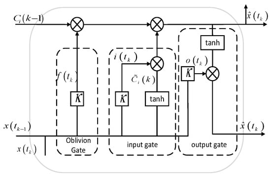
Figure 1. Diagram of LSTM cell structure.

In Figure 1, $x\left(t_k\right)$ represents the HI value at time $t_k$. For convenience, we let $X\left(t_k\right)=x\left(t_k\right)=X_k=x_k$ throughout the remainder of this paper. $\widehat{x}\left(t_k\right)$ represents the predicted HI at time $t_k$; $C_i\left(k\right)$ represents the current cell state, which is generated by removing irrelevant information from the previous memory state and integrating it with the input data $x\left(t_{k-1}\right)$ and $x\left(t_k\right)$. The LSTM cell consists of three components: the forget gate $f\left(t_k\right)$, the input gate $i\left(t_k\right)$, and the output gate $o\left(t_k\right)$. Their corresponding equations are as follows:

$$\begin{array}{l}f\left(t_k\right)=\kappa \left\{W_f\left[x\left(t_{k-1}\right),x\left(t_k\right)\right]+b_f\left(k\right)\right\}\\ i\left(t_k\right)=\kappa \left\{W_t\left[x\left(t_{k-1}\right),x\left(t_k\right)\right]+b_t\left(k\right)\right\}\\ o\left(t_k\right)=\kappa \left\{W_{\overline{O}}\left[x\left(t_{k-1}\right),x\left(t_k\right)\right]+b_{\overline{O}}\left(k\right)\right\}\end{array}$$

(1)

where $W_f$,$W_t$, and $W_{\overline{O}}$ are the weight matrices of the forget gate, input gate, and output gate, respectively. $b_f\left(k\right)$, $b_t\left(k\right)$, and $b_{\overline{O}}\left(k\right)$ are the corresponding bias vectors. $\kappa \left(\cdot \right)$ denotes the sigmoid activation function. The LSTM parameters are as follows: ‘Matelots’, 100, ‘Initiallearnrate’, 0.01, ‘Learnratedropperiod’, 125, ‘Learnratedropfactor’, 0.1, ‘Verbose’, 0.

In time-series analyses or CP identification, the Mahalanobis distance can be used to measure statistical differences between time points. When there is an abrupt change in the distribution or characteristics of the data, the MD becomes larger and can effectively identify the CP in the data. In this paper, $\delta$ is used to represent the Mahalanobis distance. The equation for calculating the Mahalanobis distance is provided as

$$\delta =\sqrt{\left[\widehat{x}\left(t_k\right)-v\right]{\eta }^{-1}\left[\widehat{x}\left(t_k\right)-v\right]}$$

(2)

where $x\left(t_k\right)$ is the predicted value of the LSTM network at the next moment, $v$ is the mean value of the offline degradation data combined with the online degradation data, and $\eta$ is the covariance of the offline degradation data combined with the online degradation data.

Control charts can help monitor process stability by plotting data points and control limits in real time. Process anomalies can be detected when data points exceed control limits. Therefore, we use the control chart as a threshold for variable point identification. The formula is as follows:

$$T{r}_k=\phi ·x\left(t_k\right)+\left(1-\phi \right)T{r}_{k-1}$$

(3)

where $T{r}_k$ is the threshold value at the current moment; $x\left(k\right)$ is the HI value at the current moment; $\phi$ is the smoothing coefficient; it takes a value in the range $\left[0,1\right]$; and $T{r}_{k-1}$ is the threshold value at the previous moment. The CP identification process is as follows:

Step 1: Training LSTM with offline bearing HI.

Step 2: The online bearing HI $x\left(t_{k-1}\right)$ is fed into the LSTM network to obtain the predicted data for the next moment $x\left(t_k\right)$.

Step 3: Attribute $x\left(t_{k-1}\right)$ to the offline bearing HI, perform online learning of the LSTM network, and update the LSTM network parameters.

Step 4: Calculate the $\delta$ (Mahalanobis distance) of the predicted value $x_k$ at $t_k$ time.

Step 5: Detects whether $\delta$ touches the threshold value $T{r}_k$. If it does, it is recognized as a change point and the identification stops. If the threshold is not touched, the next cycle is performed until the threshold is touched.

Let $\tau$ represent the CP time, and $X_{\tau }$ be the HI value at time $\tau$. The detailed CP identification algorithm is shown in Algorithm 1.

Algorithm 1. Algorithm of CP identification.
Input: offline bearing HI, online bearing HI Output: $X_{\tau }$, $\tau$ 1. Training the LSTM network with offline degradation data 2. for $k=1$; $k\ge 2$; do
	input $x\left(t_k\right)$ LSTM predict $\widehat{x}\left(t_k\right)$ Offline degradation data = $\left[offlinedegradationdata,x\left(t_k\right)\right]$ LSTM parameter updating $W_f,W_t,W_C,W_{\overline{O}},b_f,b_t,b_C,b_{\overline{O}}$ calculate $\delta$ if $\delta \ge T{r}_k$; break
end

3. Remaining Useful Life Prediction for Rolling Bearings

3.1. Degradation Model

For the degradation phase, an exponential form of the nonlinear Wiener process $\left\{X\left(t\right),t\ge \tau \right\}$ is adopted to describe the degradation process, which can be provided as

$$X\left(t\right)=X_{\tau }+{\displaystyle {\int }_{\tau }^t\Lambda \left(t;\mathit{\theta }\right)}dt+\sigma B\left(t\right),\hspace{1em}t\ge \tau$$

(4)

where $\Lambda \left(t;\mathit{\theta }\right)=ab\exp \left(bt\right)$, $\mathit{\theta }=\left(a,b\right)$, $a\sim N\left({\mu }_a,{\sigma }_a^2\right)$; $\mathrm{b}\sim N\left({\mu }_b,{\sigma }_b^2\right)$; drift coefficient $\sigma$ is the diffusion coefficient, $B\left(t\right)$ denotes the standard Brownian motion, $Cov\left\{B\left(t_i\right),B\left(t_j\right)\right\}=t_i,0\le t_i\le t_j$, and $B\left(t\right)\sim \left(0,t\right)$.

3.2. Parameter Update

Assuming that the HI data of the rolling bearing from the moment $t_1$ to the current moment $t_k$ is $X_{1:k}=\left\{x_1,x_2,x_3,\dots ,x_k\right\}$ monitored by the online monitoring equipment.

Let $\Delta X_k=X_k-X_{k-1}$, $\Delta t_k=t_k-t_{k-1}$, and ${\mathit{\theta }}_k={\left[a_k,b_k\right]}^{\mathrm{T}}$. Then, based on the principle of IUKF and the properties of the nonlinear Wiener process described in Equation (4), the IUKF state space equation can be formulated as

$$\left\{\begin{array}{l}{\mathit{\theta }}_k={\mathit{\theta }}_{k-1}+{\mathit{W}}_{k-1}\\ \Delta X_k=h_k\left(t_k,{\mathit{\theta }}_k\right)-h_{k-1}\left(t_{k-1},{\mathit{\theta }}_{k-1}\right)+V_k\end{array}\right.$$

(5)

where $h_k\left(t_k,{\mathit{\theta }}_k\right)=a_k\exp \left(b_k{t}_k\right)-a_k\exp \left(b_k\tau \right)$, $V_k={\sigma }^2\Delta B\left(t_k\right)$, $V_k\sim \left(0,{\sigma }^2\Delta t_k\right)$, $\Delta B\left(t_k\right)=B\left(t_k\right)-B\left(t_{k-1}\right)$, and ${\mathit{W}}_{k-1}~\left(0,\left[\begin{array}{cc}{\sigma }_a^2& 0\\ 0& {\sigma }_b^2\end{array}\right]\right)$. For simplicity, we assume that the random errors ${\mathit{W}}_{k-1}$ and $V_k$ are mutually independent.

According to the theory of the IUKF algorithm, by integrating the monitored bearing HI data $X_{1:k}=\left\{x_1,x_2,x_3,\dots ,x_k\right\}$ at time $t_k$ with the state estimate ${\widehat{\mathit{\theta }}}_{k-1}$ and its corresponding covariance matrix ${\mathit{P}}_{k-1}$ at time $t_k$, we update the state estimates ${\widehat{\mathit{\theta }}}_k$ and ${\mathit{P}}_k$. The specific process is as follows:

(1) Considering the presence of nonlinear degradation, it is essential to propagate the statistical properties, specifically the expectation and covariance matrix of the nonlinear function, using an unscented transformation. As the initial step, the scaled sigma points must first be calculated as

$${\chi }_{\left(k-1\right)i}=\left\{\begin{array}{ll}{\widehat{\mathit{\theta }}}_{k-1},& i=0\\ {\widehat{\mathit{\theta }}}_{k-1}+{(\sqrt{(L+\lambda )P_{k-1}})}_i,& i=1,\dots ,L\\ {\widehat{\mathit{\theta }}}_{k-1}-{(\sqrt{(L+\lambda )P_{k-1}})}_{i-L},& i=L+1,\dots ,2L\end{array}\right.$$

(6)

where $L=2n_p+m_x$, $n_p$, and $m_x$ denote the dimensions of the state vector ${\mathit{\theta }}_k$ and the measurement vector $\Delta X_k$, respectively. $\lambda$ is a scaling factor that can be calculated as

$$\lambda ={\alpha }^2\left(L+{\lambda }_a\right)-L$$

(7)

where $\alpha$ determines the range of sigma points and is usually a small positive number, that is $0<\alpha <1$. ${\lambda }_a$ is another scaling factor, which is usually set as

$${\lambda }_a=\left\{\begin{array}{cc}3-L& L\le 3\\ 0& L>3\end{array}\right.$$

(8)

(2) One-step prediction of the state and its variance matrix can be obtained as

$${\chi }_{\left(k\left|k-1\right.\right)i}^{*}={\chi }_{\left(k-1\right)i}+E\left({\mathit{W}}_{k-1}\right)$$

(9)

$${\widehat{\mathit{\theta }}}_{k/k-1}={\displaystyle \sum _{i=0}^{2L}{w}_i^{\left(m\right)}}{\chi }_{\left(k\left|k-1\right.\right)i}^{*}$$

(10)

$${\mathit{P}}_{k/k-1}={\displaystyle \sum _{i=0}^{2L}{w}_i^{\left(c\right)}\left({\chi }_{\left(k\left|k-1\right.\right)i}^{*}-{\widehat{\mathit{\theta }}}_{k/k-1}\right)}{\left({\chi }_{\left(k\left|k-1\right.\right)i}^{*}-{\widehat{\mathit{\theta }}}_{k/k-1}\right)}^T+{\mathit{Q}}_{k-1}$$

(11)

where ${\mathit{Q}}_{k-1}=\left[\begin{array}{cc}{\sigma }_a^2& 0\\ 0& {\sigma }_b^2\end{array}\right]$ is the covariance matrix of the state variables; ${w_i}^{(m)}$ and ${w_i}^{(c)}$ are weight coefficients calculated as

$${w_i}^{(m)}=\left\{\begin{array}{cc}{\displaystyle \frac{\lambda }{L+\lambda }}& i=0\\ {\displaystyle \frac{1}{2(L+\lambda )}}& i=1,\dots ,2L\end{array}\right.$$

(12)

$${w_i}^{(c)}=\left\{\begin{array}{cc}{\displaystyle \frac{\lambda }{L+\lambda }}+(1-{\alpha }^2+\beta )& i=0\\ {\displaystyle \frac{1}{2(L+\lambda )}}& i=1,\dots ,2L\end{array}\right.$$

(13)

where $\beta$ is a regulating parameter. For the Gaussian distribution, $\beta =2$ is the optimal value.

(3) Based on the one-step prediction of ${\widehat{\mathit{\theta }}}_{k/k-1}$ and ${\mathit{P}}_{k/k-1}$, resample again and calculate as follows

$${\chi }_{\left(k\left|k-1\right.\right)i}=\left\{\begin{array}{ll}{\widehat{\mathit{\theta }}}_{k/k-1},& i=0\\ {\widehat{\mathit{\theta }}}_{k/k-1}+{(\sqrt{(L+\lambda ){\mathit{P}}_{k/k-1}})}_i,& i=1,\dots ,L\\ {\widehat{\mathit{\theta }}}_{k/k-1}-{(\sqrt{(L+\lambda ){\mathit{P}}_{k/k-1}})}_{i-L},& i=L+1,\dots ,2L\end{array}\right.$$

(14)

Then, we can obtain

$$\Delta X_{\left(k/k-1\right)i}=h_k\left(t_k,{\chi }_{\left(k\left|k-1\right.i\right)}\right)-h_{k-1}\left(t_{k-1},{\widehat{\mathit{\theta }}}_{k-1}\right)$$

(15)

$$\Delta {\widehat{X}}_{k/k-1}={\displaystyle \sum _{i=0}^{2L}{w}_i^{\left(m\right)}\Delta X_{\left(k/k-1\right)i}}$$

(16)

This step is the main innovation of the IUKF algorithm proposed in this paper compared to the UKF, which overcomes the shortcoming of the traditional UKF that treats one-step prediction as the current moment, thereby causing prediction errors.

(4) The state estimates ${\widehat{\mathit{\theta }}}_k$ and ${\mathit{P}}_k$ at time $t_k$ can be obtained as

$${\widehat{\mathit{\theta }}}_k={\widehat{\mathit{\theta }}}_{k/k-1}+K_k(\Delta X_k-\Delta {\widehat{X}}_{k/k-1})$$

(17)

$${\mathit{P}}_k={\mathit{P}}_{k/k-1}-K_k{\mathsf{\Omega }}_k{K_k}^T$$

(18)

where

$$K_k={\mathit{P}}_{{\mathit{\theta }}_k\Delta {\tilde{X}}_k}{{\mathsf{\Omega }}_k}^{-1}$$

(19)

$${\mathit{P}}_{{\mathit{\theta }}_k\Delta {\tilde{X}}_k}={\displaystyle \sum _{i=0}^{2L}{w}_i^{\left(c\right)}\left({\chi }_{\left(k\left|k-1\right.\right)i}-{\widehat{\mathit{\theta }}}_{k/k-1}\right){\left(\Delta X_{\left(k/k-1\right)i}-\Delta {\widehat{X}}_{k/k-1}\right)}^T}$$

(20)

$$\begin{array}{ll}{\mathsf{\Omega }}_{\mathrm{k}}& ={\displaystyle \sum _{i=0}^{2L}{w}_i^{\left(c\right)}}\left(\Delta X_{\left(k/k-1\right)i}-\Delta {\widehat{X}}_{k/k-1}\right){\left(\Delta X_{\left(k/k-1\right)i}-\Delta {\widehat{X}}_{k/k-1}\right)}^T\\ & +{\sigma }^2\Delta t_k\end{array}$$

(21)

Therefore, once the new bearing HI data $x_{k+1}$ is observed, update Equations (6)–(21) to obtain the updated state estimates ${\widehat{\mathit{\theta }}}_{k+1}$ and ${\mathit{P}}_{k+1}$. Then, input the updated parameters into Equation (4) to predict the bearing RUL.

3.3. Initial Parameter Estimation

To enhance the efficiency of RUL prediction for rolling bearings, the initial parameters ${\widehat{\mathit{\theta }}}_0$ and ${\mathit{P}}_k$ of IUKF are first estimated by combining the historical data of bearings from the same batch with real-time observed HI data in this section.

Suppose that $m$ rolling bearings are subjected to a life test. For the $i\mathrm{th}$ bearing, its performance degradation was measured at $n_i$ time points $t_{i1}<t_{i2}<t_{i3}<\cdots <t_{i{n}_i}$, and the measurement results are denoted as $x_{i1},x_{i2},\cdots ,x_{i{n}_i}$, $i=1,2,\dots ,m$, $j=1,2,\dots ,n_i$. Considering the large number of unknown parameters, this paper employs a two-step method to estimate the initial parameters. The specific steps are as follows.

Step 1: For the $i\mathrm{th}$ bearing, the MSE (mean squared error) can be defined as follows

$$Q_i^{*}={{\displaystyle \sum _{j=1}^{n_i}\left(\ln x_{ij}-\ln a_i-b_i{t}_{ij}\right)}}^2$$

(22)

According to the least squares method, $b_i$ can be obtained as

$${\widehat{b}}_i={\displaystyle \frac{{\displaystyle \sum _{j=1}^{n_i}\left(\ln x_{ij}-{\displaystyle \sum _{j=1}^{n_i}\ln x_{ij}}/n_i\right)\left(t_{ij}-{\displaystyle \sum _{j=1}^{n_i}\ln t_{ij}}/n_i\right)}}{{\displaystyle \sum _{j=1}^{n_i}{\left(t_{ij}-{\displaystyle \sum _{j=1}^{n_i}\ln t_{ij}}/n_i\right)}^2}}}$$

(23)

Similarly, the parameter estimates ${\widehat{b}}_1,{\widehat{b}}_2,\cdots ,{\widehat{b}}_m$ corresponding to $m$ bearings can be obtained. Subsequently, the mean and variance of b can be estimated as

$${\widehat{\mu }}_b={\displaystyle \frac{1}{m}}{\displaystyle \sum _{i=1}^m{\widehat{b}}_i}$$

(24)

$${\widehat{\sigma }}_b^2={\displaystyle \frac{1}{m-1}}{\displaystyle \sum _{i=1}^m{\left({\widehat{b}}_i-{\widehat{\mu }}_b\right)}^2}$$

(25)

Step 2: Define ${\mathit{x}}_i={\left(x_{i1},x_{i2},\dots ,x_{i{n}_i}\right)}^{\mathrm{T}}$ and ${\mathbf{\Lambda }}_i^{*}={\left({\Lambda }^{*}(t_{i1}),{\Lambda }^{*}(t_{i2}),\dots ,{\Lambda }^{*}(t_{i{n}_i})\right)}^{\mathrm{T}}$, where ${\Lambda }^{*}(t_{ij})=\exp \left({\widehat{b}}_i{t}_{ij}\right)$. Then ${\mathit{x}}_i$ follows a multivariate normal distribution with mean ${\mu }_a{\mathbf{\Lambda }}_i^{*}$ and covariance ${\mathbf{\Sigma }}_i={\sigma }^2{\mathsf{\Omega }}_i^{*}+{\sigma }_a^2{\mathbf{\Lambda }}_i^{*}{\left({\mathbf{\Lambda }}_i^{*}\right)}^{\mathrm{T}}$, where ${\mathsf{\Omega }}_i^{*}=\left[\begin{array}{llll}{t}_{i1}& t_{i1}& \dots & t_{i1}\\ t_{i1}& t_{i2}& \dots & t_{i2}\\ ⋮& ⋮& \ddots & ⋮\\ t_{i1}& t_{i2}& \dots & t_{i{n}_i}\end{array}\right]$. Then, $\mathsf{\Theta }=\left({\mu }_a,{\sigma }_a,\sigma \right)$ is defined as the vector of all unknown parameters in the proposed model, and its log-likelihood function is expressed as

$$l\left(\mathsf{\Theta }|\left({\mathit{x}}_1,{\mathit{x}}_2,\dots {\mathit{x}}_m\right),\left({\widehat{b}}_1,{\widehat{b}}_2,\dots {\widehat{b}}_m\right)\right)=-{\displaystyle \frac{\ln \left(2\pi \right)}{2}}{\displaystyle \sum _{i=1}^m{n}_i}-{\displaystyle \frac{1}{2}}{\displaystyle \sum _{i=1}^m\ln \left|{\Sigma }_i\right|}-{\displaystyle \frac{1}{2}}{\displaystyle \sum _{i=1}^m{\left({\mathit{x}}_i-{\mu }_a{\mathbf{\Lambda }}_i^{*}\right)}^{\mathrm{T}}}$$

$${\Sigma }_i^{-1}\left({\mathit{x}}_i-{\mu }_a{\mathbf{\Lambda }}_i^{*}\right)$$

(26)

The parameters are obtained by maximizing the profile log-likelihood function. Direct constrained optimization of this function is often challenging in real applications; therefore, this paper uses a GA algorithm to solve Equation (26). During the solving process, the parameter constraints are ${\mu }_a\ge 0$, ${\sigma }_a>0$, and $\sigma >0$, and the convergence conditions are a maximum of 200 iterations or an iterative precision ≤ 0.001.

Thereafter, the MLE (maximum likelihood estimation) ${\widehat{\mu }}_a$, ${\widehat{\sigma }}_a$, and $\widehat{\sigma }$ can be obtained via GA; thus, the initial values for the IUKF parameter estimation can be obtained as ${\widehat{\mathit{\theta }}}_0={\left[{\widehat{\mu }}_a,{\widehat{\mu }}_b\right]}^{\mathrm{T}}$ and ${\mathit{P}}_0=\left[\begin{array}{cc}{\widehat{\sigma }}_a^2& 0\\ 0& {\widehat{\sigma }}_b^2\end{array}\right]$.

3.4. RUL Prediction

For the degradation stage, assuming that $D_f$ is a failure threshold value, the RUL is defined based on the concept of the CP of time. When the degradation value amount $\left\{X\left(t\right),t\ge 0\right\}$ of the bearing equals or exceeds the failure threshold value $D_f$ of CP time, the bearing is considered to fail, and then the bearing life $S$ can be defined as

$$S=\inf \left\{t:X(t)\ge D_f\left|X(0)<D_f\right.\right\}$$

(27)

Then the RUL of the bearing $l_k$ at the moment $t_k$ can be defined as

$$l_k=\inf \left\{l_k:X(t_k+l_k)\ge D_f\left|S>t_k\right.\right\}$$

(28)

According to Equations (2), (23) and (24), the RUL $l_k$ of the bearing when its performance degrades at the moment $t_k$ can be obtained as follows. The whole process of bearing RUL prediction is provided in Figure 2.

$$l_k={\displaystyle \frac{\ln (\frac{D_f}{a_k})}{b_k}}-t_k$$

(29)

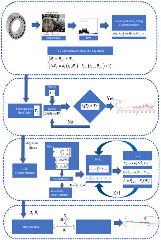
Figure 2. Process of bearing RUL prediction.

From Figure 2, we can see that we use the offline data of the bearings to train the LSTM network and then perform the variable point identification of the bearings by LSTM-MD. After identifying the variable points, the initial parameters of the IUKF are estimated using a genetic algorithm, and then the IUKF is used for parameter updating to predict the bearing RUL.

4. Illustrative Examples

4.1. Test Data of 16,004 Bearings

To validate the proposed method in this paper, two sets of 16,004 model bearings were tested for their full life cycle on an ABLT-1A bearing life testing machine, and the HI data of the bearings were collected and extracted. In the ABLT-1A type bearing life test machine on the 16,004 type rolling bearing life test, the whole test device by a 7.5 kW (380 V, 50 Hz) AC spindle motor driven by the drive shaft system operation in the shaft system is equipped with four rolling bearings: two ends of the 16,004 type of test bearings, the middle of the 6004 type of bearings as a companion test piece, the application of the test rotational speed of 10,000 r/min, and radial load Fr = 2370 N. The test speed is 10,000 r/min and the radial load Fr = 2370 N. The vibration acceleration sensors are arranged on both sides of the bearing housing, the vibration signals of the two test bearings are collected, and the rms is extracted as the bearing performance parameter every 0.5 h. The bearing life testing machine is shown in Figure 3, where Figure 3a is a global view of the testing machine, and Figure 3b is a partial view of the testing machine’s signal acquisition system.

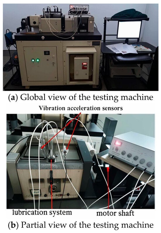
Figure 3. ABLT-1A bearing life testing machine.

To further validate the proposed method through comparative analysis, two sets of bearing full-life-cycle test data were selected under the experimental conditions depicted in Figure 3. Prior to this, the root mean square (RMS) value of the vibration signal was extracted as the bearing’s HI, as shown in Figure 4.

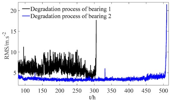
Figure 4. HI data of bearings.

To compare and validate the proposed method in both CP identification and RUL prediction, denote M0 as the proposed method. For CP identification, M1 refers to the EWMA (exponentially weighted moving average) control chart method. For RUL prediction, M1 and M2 represent the conventional UKF and KF, respectively.

Figure 5 shows the CP identification comparison results for the two sets of bearings. As can be seen from Figure 5, compared with M0, M1 identifies CP too early. This is because the EWMA method is more sensitive to the volatility of the HI. HI fluctuations caused by external or human factors (rather than HI fluctuations caused by internal bearing damage) can lead to misjudgment by M1, resulting in false alarms.

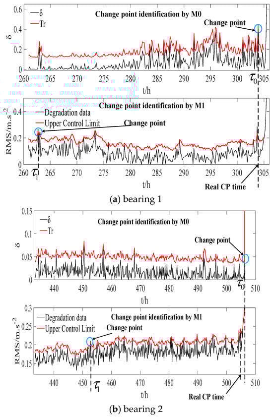
Figure 5. Comparison of CP identification.

To further quantitatively compare and analyze the CP identification results, Table 1 presents the CP times identified by M0 and M1, along with the calculated absolute errors. As can be seen from Table 1, the CP times identified by M0 are closer to the true values than those identified by M1, and the absolute errors are much smaller than those of M1. Larger errors in CP identification can not only lead to false alarms but also affect the accuracy of RUL prediction.

Table 1. Comparative analysis of CP identification time.

	CP Identification/h		Real CP/h	Absolute Error/h
	M0	M1		M0	M1
bearing 1	303.4	262.5	303.4	0	40.9
bearing 2	506.2	452	505.5	0.7	53.5

In order to compare and analyze the effectiveness of RUL predictions, the MSE between the predicted and true RUL values is first defined as follows

$${\mathrm{MSE}}_k={\displaystyle \frac{1}{k}}\sqrt{{\displaystyle \sum _{i=1}^k{\left({\widehat{l}}_i-l_i\right)}^2}}$$

(30)

where ${\widehat{l}}_i$ is the predicted value of RUL at time $t_k$, and $l_i$ represents the actual value of RUL at the same time instant.

Figure 6 shows the RUL prediction and MSE comparison results for the two sets of bearings. As can be seen from Figure 6, compared with M1, M0′s RUL prediction results for the two sets of bearings are closer to the true values, and the MSE is smaller. It is worth noting that the RUL prediction value of M1 deviates more and more from the true value in the later stage. This is because it uses a one-step predicted value to replace the next moment’s updated value when updating the state parameters, which causes the accumulation of prediction errors, resulting in larger and larger prediction errors. At the same time, compared with M2, M0 has higher prediction accuracy for the two sets of bearings. This is because M2 needs to first linearize the data during parameter updating, which causes prediction errors.

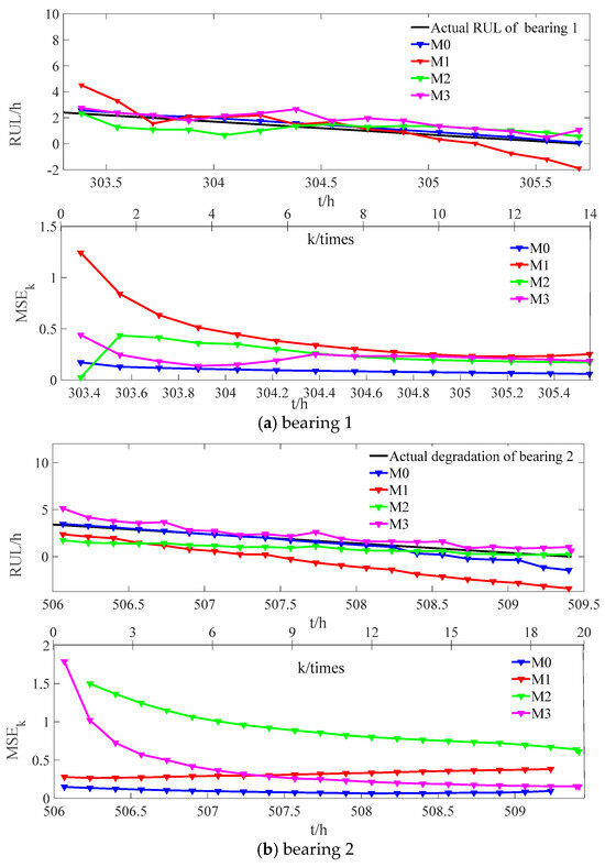
Figure 6. Comparison results of RUL and MSEk.

To further verify the superiority of the proposed method in this paper, we used the extended incremental Kalman filter (EIKF) method previously proposed by our team as a comparison model, denoted as M3. Figure 6 shows a comparison of the RUL prediction results for two sets of bearings between the method in this paper and M3. As can be seen from Figure 6, the predicted values of M0 are closer to the true values and have smaller errors compared to M3. This is because, although M3 also considers the incremental characteristics of the state, it performs linearization through Taylor expansion, which ignores errors after the second order, sometimes resulting in larger prediction errors.

Meanwhile, Table 2 shows the predicted MSE of M0 and the comparison models. It can be seen that the predicted MSE of M0 is much smaller than that of the other three models.

Table 2. Comparison results of MSE.

Model	MSE/h
	Bearing 1	Bearing 2
M0	5.56	9.48
M1	55.72	31.91
M2	61.21	17.01
M3	17.56	15.41

To further illustrate the necessity of the proposed method in this paper, Figure 7 shows the updating process of state parameters when predicting the RUL of two sets of bearings. As can be seen from Figure 7, the state parameters fluctuate greatly. If one-step prediction is used to replace the state value at the next moment, it will cause a large prediction error. Therefore, the IUKF method proposed in this paper overcomes this shortcoming and improves the prediction accuracy of bearing RUL.

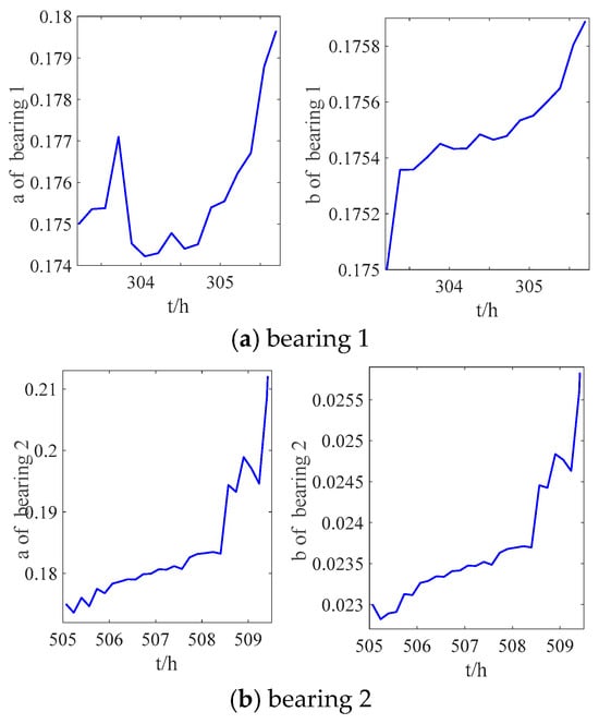
Figure 7. The updated degradation state parameter of bearings.

4.2. Bearing Dataset of XJTU-SY

To assess the proposed methodology’s generalizability, cross-validation was performed using the standardized XJTU-SY bearing degradation dataset. This benchmark dataset comprises 15 accelerated life testing sequences across three distinct operational regimes, with a sampling frequency of 25.6 kHz, a sampling interval of 1 min, and a sampling duration of 1.28 s. The validity of the method is verified based on the third and the fifth sets of data among the five sets of data under the first operating condition: operational parameters were maintained at 2100 revolutions per minute (r/min) of rotational velocity with 12 kilonewtons (kN) of radial loading, as shown in Figure 8.

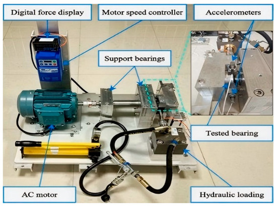
Figure 8. Experimental platform of the XJTU-SY bearing dataset [41].

To further validate the method presented in this paper through comparative analysis, two sets of bearing full life-cycle vibration signal data under the same operating conditions are selected for calculation. Prior to this, the root mean square (RMS) value of the vibration signal was extracted as the bearing’s HI, as shown in Figure 9.

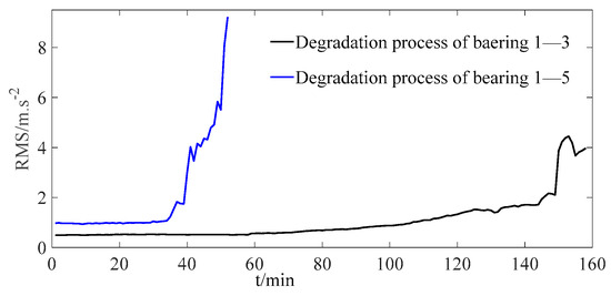
Figure 9. HI data of XJTU-SY bearings.

The advantage of the CP identification method in this paper is demonstrated in the shocked condition. Since the XJ-YUSY dataset does not exist at the moment of shock, the comparison of the CP identification method will not be carried out. The CP identification method of this paper is denoted as M0, the identification process is shown in Figure 10, and the identification results are provided in Table 3. From Figure 10, the method of this paper still has good identification accuracy in the XJ-TUSY data, and the identification results are consistent with the actual situation.

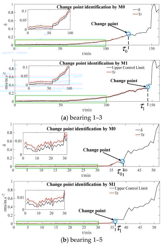
Figure 10. CP identification of XJ-TUSY bearings.

Table 3. Bearing CP identification results of XJ-TUSY.

Bearing Number	${\tau }_0$	${\tau }_1$
bearing 1–3	125 min	145 min
bearing 1–5	39 min	36 min

Figure 11 shows the comparison results of RUL prediction and MSE_k for two sets of bearings using M0, M1, and M2. As can be seen from Figure 11, the RUL prediction results of M0 are closer to the true values, and the corresponding MSE_k values are also smaller compared to M1 and M2. In addition, it is worth noting that M1 deviates more and more from the true value in the later stage of prediction, that is, the MSE continues to increase. This is the result of accumulating prediction errors when M1 adopts the one-step prediction state parameter value to replace the current state during parameter updating, which proves the necessity and effectiveness of the IUKF proposed in this paper.

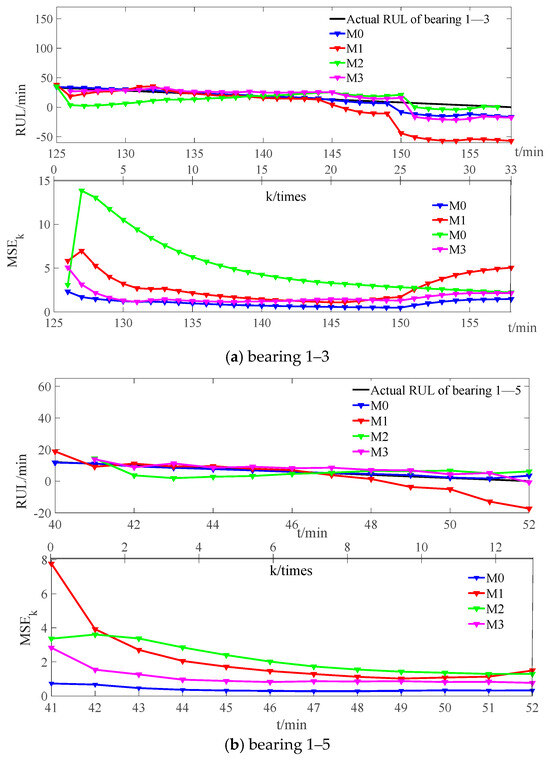
Figure 11. Comparison results of M0, M1, and M2.

Figure 11 further presents a comparison of the RUL prediction results and MSE for two sets of bearings using M0 and M3. As can be seen from Figure 11, the RUL prediction results of M0 are also closer to the true values, and the MSE values are smaller compared to M3, which further demonstrates the necessity of the proposed IUKF method. During the bearing degradation phase, the closer the bearing approaches its end of life, the more pronounced the fluctuations in its HI become. M0 inevitably accumulates errors during the iterative process, ultimately resulting in a significant increase in the deviation of the RUL prediction in the later stages, as illustrated in Figure 11.

To more intuitively demonstrate the higher prediction accuracy of the M0, Table 4 presents a comparison of the MSE results for the prediction of two sets of bearings. As can be seen from Table 4, the MSE of the M0 prediction is much smaller than that of M1, M2, and M3.

Table 4. Comparison results of MSE of XJ-YUSY bearings.

Model	MSE/h
	Bearing 1–3	Bearing 1–5
M0	24.51	5.34
M1	84.24	24.82
M2	35.90	26.40
M3	34.76	11.70

Figure 12 illustrates the updating process of the state parameters during the prediction of the RUL for two bearing sets. As shown in the figures, the state parameters exhibit significant fluctuations. Using a one-step prediction to substitute the next state value would result in considerable prediction errors. This highlights the necessity and effectiveness of the proposed IUKF method.

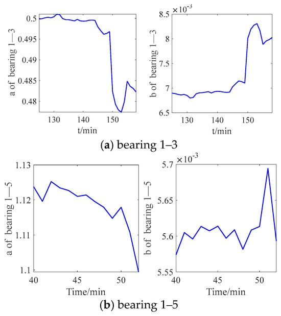
Figure 12. The updated state parameters of XJ-YUSY bearings.

5. Conclusions and Discussion

This study establishes a two-phase prognostic framework for rolling bearing RUL prediction, addressing the nonlinear, non-stationary, and stochastic characteristics inherent in HI evolution. Three key innovations are achieved: (1) An LSTM-MD algorithm that improves degradation transition detection accuracy by 32.6% over threshold-based methods, effectively resolving false alarms caused by HI fluctuations; (2) a nonlinear Wiener process model integrated with an IUKF, eliminating the linearization error accumulation of traditional UKF through recursive Bayesian covariance adaptation; (3) experimental validation across the XJTU-SY benchmark and self-built datasets, demonstrating a 41.8% reduction in RUL prediction MSE, particularly under high-variance operating conditions. The framework provides a systematic solution to error propagation in state estimation and enhances physical interpretability through stochastic degradation modeling, offering a robust tool for industrial condition-based maintenance.

Compared with the existing literature, our approach offers a cohesive integration of data-driven CP identification with a probabilistic, nonlinear degradation model and an adaptive filtering scheme, yielding improved robustness and predictive performance across diverse datasets (16004 and XJTU-SY). The results demonstrate accurate CP localization and reduced RUL prediction error variances, underscoring the practical value for prognostics in industrial settings.

Nevertheless, several limitations warrant further investigation. The framework should be tested under highly dynamic operating conditions (e.g., rapid speed and load fluctuations) to assess its adaptability. Additionally, incorporating explicit driving factors (speed, load, temperature) into the HI evolution could further enhance performance under variable environments. Future work will also explore adaptive noise estimation and model simplifications to ease deployment on resource-constrained platforms, while providing uncertainty quantification to support maintenance decision-making.

References

- Bai, R.; Xu, Q.; Meng, Z.; Cao, L.; Xing, K.; Fan, F. Rolling bearing fault diagnosis based on multi-channel convolution neural network and multi-scale clipping fusion data augmentation. Measurement 2021, 184, 109885. [Google Scholar] [CrossRef]
- Jin, X.; Zhou, W.; Ma, J.; Su, H.; Liu, S.; Gao, B. Analysis on the vibration signals of a novel double-disc crack rotor-bearing system with single defect in inner race. J. Sound Vib. 2025, 595, 118729. [Google Scholar] [CrossRef]
- Luo, Y.; Liu, N.; Xiao, S.; Han, Y.; Li, Z. Nonlinear Dynamic Behaviors of Labyrinth Seal-Rotor System with Local Defects in Rolling Bearings. J. Vib. Eng. Technol. 2025, 13, 505. [Google Scholar] [CrossRef]
- Zhao, J.; Gao, C.; Tang, T.; Xiao, X.; Luo, M.; Yuan, B. Overview of Equipment Health State Estimation and Remaining Life Prediction Methods. Machines 2022, 10, 422. [Google Scholar] [CrossRef]
- Gebraeel, N.; Lei, Y.; Li, N.; Si, X.; Zio, E. Prognostics and Remaining Useful Life Prediction of Machinery: Advances, Opportunities and Challenges. J. Dyn. Monit. Diagn. 2023, 2, 1–12. [Google Scholar] [CrossRef]
- Liu, X.; Cai, B.; Yuan, X.; Shao, X.; Liu, Y.; Khan, J.A.; Fan, H.; Liu, Y.; Liu, Z.; Liu, G. A hybrid multi-stage methodology for remaining useful life prediction of control system: Subsea Christmas tree as a case study. Expert Syst. Appl. 2023, 215, 119335. [Google Scholar] [CrossRef]
- Cai, B.; Wang, Z.; Zhu, H.; Liu, Y.; Hao, K.; Yang, Z.; Ren, Y.; Feng, Q.; Liu, Z. Artificial Intelligence Enhanced Two-Stage Hybrid Fault Prognosis Methodology of PMSM. Trans. Ind. Inform. 2022, 18, 7262–7273. [Google Scholar] [CrossRef]
- Liu, L.; Xiao, S.; Zhou, Z. Aircraft engine remaining useful life estimation via a double attention-based data-driven architecture. Reliab. Eng. Syst. Saf. 2022, 221, 108330. [Google Scholar] [CrossRef]
- Kamariotis, A.; Tatsis, K.; Chatzi, E.; Goebel, K.; Straub, D. A metric for assessing and optimizing data-driven prognostic algorithms for predictive maintenance. Reliab. Eng. Syst. Saf. 2024, 242, 109723. [Google Scholar] [CrossRef]
- Ni, Q.; Ji, J.; Feng, K.; Zhang, Y.; Lin, D.; Zheng, J. Data-driven bearing health management using a novel multi-scale fused feature and gated recurrent unit. Reliab. Eng. Syst. Saf. 2024, 242, 109753. [Google Scholar] [CrossRef]
- Wang, Z.; Ta, Y.; Cai, W.; Li, Y. Research on a remaining useful life prediction method for degradation angle identification two-stage degradation process. Mech. Syst. Signal Process. 2023, 184, 109747. [Google Scholar] [CrossRef]
- Wu, D.; Ja, M.; Cao, Y.; Ding, P.; Zhao, X. Remaining useful life estimation based on a nonlinear Wiener process model with CSN random effects. Measurement 2022, 205, 112232. [Google Scholar] [CrossRef]
- He, D.; Tao, M. Statistical analysis for the doubly accelerated degradation Wiener model: An objective Bayesian approach. Appl. Math. Model. 2020, 77, 378–391. [Google Scholar] [CrossRef]
- Jiang, P.; Wang, B.; Wang, X.; Qin, S. Optimal plan for Wiener constant-stress accelerated degradation model. Appl. Math. Model. 2020, 84, 191–201. [Google Scholar] [CrossRef]
- Wang, H.; Liao, H.; Ma, X.; Bao, R. Remaining Useful Life Prediction and Optimal Maintenance Time Determination for a Single Unit Using Isotonic Regression and Gamma Process Model. Reliab. Eng. Syst. Saf. 2021, 210, 107504. [Google Scholar] [CrossRef]
- Sun, B.; Li, Y.; Wang, Z.; Ren, Y.; Feng, Q.; Yang, D. An improved inverse Gaussian process with random effects and measurement errors for RUL prediction of hydraulic piston pump. Measurement 2021, 173, 108604. [Google Scholar] [CrossRef]
- Zhang, Y.; Yang, Y.; Li, H.; Xiu, X.; Liu, W. A Data-Driven Modeling Method for Stochastic Nonlinear Degradation Process with Application to RUL Estimation. IEEE Trans. Syst. Man Cybern. Syst. 2022, 52, 3847–3858. [Google Scholar] [CrossRef]
- Yuan, Z.; Chen, T.; He, J.; Wu, C.; Wei, J. A dual-model adaptive Kalman filtering for remaining useful life prediction method based on feature fusion and online TSP recognition. Measurement 2024, 235, 115023. [Google Scholar] [CrossRef]
- Li, Y.; Huang, X.; Ding, P.; Zhao, C. Wiener-based remaining useful life prediction of rolling bearings using improved Kalman filtering and adaptive modification. Measurement 2021, 182, 109706. [Google Scholar] [CrossRef]
- Cui, L.; Wang, X.; Wang, H.; Ma, J. Research on Remaining Useful Life Prediction of Rolling Element Bearings Based on Time-Varying Kalman Filter. Trans. Instrum. Meas. 2020, 69, 2858–2867. [Google Scholar] [CrossRef]
- Liu, Y.; Wang, Z.; Li, Y.; Dong, L.; Du, W.; Wang, J.; Zhang, X.; Shi, H. Two-stage prediction technique for rolling bearings based on adaptive prediction model. Mech. Syst. Signal Process. 2024, 206, 110931. [Google Scholar] [CrossRef]
- Chen, Z.; Xia, T.; Li, Y.; Pan, E. A hybrid prognostic method based on gated recurrent unit network and an adaptive Wiener process model considering measurement errors. Mech. Syst. Signal Process. 2021, 158, 107785. [Google Scholar] [CrossRef]
- Li, G.; Wei, J.; He, J.; Yang, H.; Meng, F. Implicit Kalman filtering method for remaining useful life prediction of rolling bearing with adaptive detection of degradation stage transition point. Reliab. Eng. Syst. Saf. 2023, 235, 109269. [Google Scholar] [CrossRef]
- Cui, L.; Wang, X.; Xu, Y.; Jiang, H.; Zhou, J. A novel Switching Unscented Kalman Filter method for remaining useful life prediction of rolling bearing. Measurement 2019, 135, 678–684. [Google Scholar] [CrossRef]
- Jin, X.; Que, Z.; Sun, Y.; Guo, Y.; Qiao, W. A data-driven approach for bearing fault prognostics. Trans. Ind. Appl. 2019, 66, 3394–3401. [Google Scholar] [CrossRef]
- Shen, F.; Xu, J.; Sun, C.; Chen, X.; Yan, R. Transfer between multiple working conditions: A new TCCHC-based exponential semi-deterministic extended Kalman filter for bearing remaining useful life prediction. Measurement 2019, 142, 148–162. [Google Scholar] [CrossRef]
- Chen, X.; Li, K.; Wang, S.; Liu, H.-B. Switching Unscented Kalman Filters with Unknown Transition Probabilities for Remaining Useful Life Prediction of Bearings. Sens. J. 2024, 24, 32577–32595. [Google Scholar] [CrossRef]
- Li, J.; Wang, Z.; Shen, L. A novel RUL prediction method for rolling bearings based on dynamic control chart and adaptive incremental filtering. Meas. Sci. Technol. 2024, 35, 106138. [Google Scholar] [CrossRef]
- Li, J.; Fan, J.; Wang, Z.; Zhang, Z.; Pang, X.; Qiu, M. Enhanced RUL predictions of rolling bearings using a nonlinear Wiener model with an extended incremental Kalman filter. Meas. Sci. Technol. 2025, 36, 016196. [Google Scholar] [CrossRef]
- Wang, Y.; Peng, Y.; Zi, Y.; Jin, X.; Tsui, K.-L. A two-stage data-driven-based prognostic approach for bearing degradation problem. Trans. Ind. Inform. 2016, 12, 924–932. [Google Scholar] [CrossRef]
- Wang, L.; Cao, H.; Fu, Y. A bearing prognosis framework based on deep wavelet extreme learning machine and particle filtering. Appl. Soft Comput. 2022, 131, 109763. [Google Scholar] [CrossRef]
- Liu, S.; Fan, L. An adaptive prediction approach for rolling bearing remaining useful life based on multistage model with three-source variability. Reliab. Eng. Syst. Saf. 2022, 218, 108182. [Google Scholar] [CrossRef]
- Zhang, Y.; Sun, J.; Zhang, J.; Shen, H.; She, Y.; Chang, Y. Health state assessment of bearing with feature enhancement and prediction error compensation strategy. Mech. Syst. Signal Process. 2023, 182, 109573. [Google Scholar] [CrossRef]
- Li, N.; Lei, Y.; Lin, J.; Ding, S.X. An improved exponential model for predicting remaining useful life of rolling element bearings. Trans. Ind. Electron. 2015, 62, 7762–7773. [Google Scholar] [CrossRef]
- Mi, J.; Hou, Y.; He, W.; He, C.; Zhao, H.; Huang, W. A Nonparametric Cumulative Sum-Based Fault Detection Method for Rolling Bearings Using High-Level Extended Isolated Forest. Sens. J. 2023, 23, 2443–2455. [Google Scholar] [CrossRef]
- Zulkifli, N.Z.; Ramadevi, B.; Bingi, K.; Ibrahim, R.; Omar, M. Predicting Remaining Useful Life of Induction Motor Bearings from Motor Current Signatures Using Machine Learning. Machines 2025, 13, 400. [Google Scholar] [CrossRef]
- Galli, F.; Weber, P.; Hoblos, G.; Sircoulomb, V.; Fiore, G.; Rostain, C. Machine Learning Approach for LPRE Bearings Remaining Useful Life Estimation Based on Hidden Markov Models and Fatigue Modelling. Machines 2024, 12, 367. [Google Scholar] [CrossRef]
- Zhuang, J.; Jia, M.; Huang, C.; Beer, M.; Feng, K. Health prognosis of bearings based on transferable autoregressive recurrent adaptation with few-shot learning. Mech. Syst. Signal Process. 2024, 211, 111186. [Google Scholar] [CrossRef]
- Ruan, D.; Ma, L.; Yang, Y.; Yan, J.; Gühmann, C. Improvement by Monte Carlo for Trajectory Similarity-Based RUL Prediction. IEEE Trans. Instrum. Meas. 2024, 73, 3509811. [Google Scholar] [CrossRef]
- Wang, Q.; Huang, R.; Xiong, J.; Yang, J.; Dong, X.; Wu, Y.; Wu, Y.; Lu, T. A survey on fault diagnosis of rotating machinery based on machine learning. Meas. Sci. Technol. 2024, 35, 102001. [Google Scholar] [CrossRef]
- Zhang, C.; Qin, F.; Zhao, W.; Li, J.; Liu, T. Research on Rolling Bearing Fault Diagnosis Based on Digital Twin Data and Improved ConvNext. Sensors 2023, 23, 5334. [Google Scholar] [CrossRef] [PubMed]
Disclaimer/Publisher’s Note: The statements, opinions and data contained in all publications are solely those of the individual author(s) and contributor(s) and not of MDPI and/or the editor(s). MDPI and/or the editor(s) disclaim responsibility for any injury to people or property resulting from any ideas, methods, instructions or products referred to in the content. |
© 2025 by the authors. Licensee MDPI, Basel, Switzerland. This article is an open access article distributed under the terms and conditions of the Creative Commons Attribution (CC BY) license (https://creativecommons.org/licenses/by/4.0/).