Dynamic Modeling and Performance Evaluation of a 5-DOF Hybrid Robot for Composite Material Machining

Abstract

Dynamic performance is an important performance of robots used for machine processing. This paper studies the dynamic modeling and evaluation method of a 5-DOF (Degree of Freedom) hybrid robot used in aerospace composite material processing. With the consideration of the dynamics of the serial part, the complete dynamic model of the hybrid robot is established based on the virtual work principle. In addition to the widely considered acceleration term, a dynamic performance evaluation index that comprehensively considers the acceleration term, velocity term and gravity term in the dynamic model is proposed. Using the dynamic performance index, the effect of the placement direction of the robot and the arrangement of the double symmetric limbs on robot dynamics are investigated. The results indicate that the vertical placement is beneficial to the dynamics of the hybrid robot, and the arrangement of double symmetric limbs has different effects on different limbs.

1. Introduction

Because of high stiffness and good bearing capacity, parallel mechanisms have wide application prospects in the machining field [1,2,3,4]. Despite these advantages, parallel mechanisms also have the obvious disadvantage of poor dexterity and small workspace [5,6,7,8]. Redundancy has been shown to improve the mechanical performance of parallel mechanisms, but control challenges also arise with the introduction of redundancy [9]. On the contrary, serial robots generally have the advantages of good dexterity and a big workspace. The hybrid robot with the merits of both parallel robot and serial robot has great potential in polishing operation [10], pose adjusting system [11], prosthesis and external exoskeleton [12], machining field [13,14,15], etc. One of the most representative hybrid robots is the 5-DOF hybrid robot that consists of a 3-DOF 2R1T (two rotational DOFs and one translational DOF) parallel mechanism and a 2-DOF serial rotating head, such as the Ecospeed [16], Exechon [17] and Tricept [18,19] robots.

Dynamic performance is of great importance for the robots, especially when the robots are applied in machining field, which requires high dynamic performance [20,21]. It is necessary to establish a dynamic model to study the dynamic performance. However, the hybrid robot not only combines the merits of serial and parallel mechanisms but also inherits their complexity of kinematics [22]. Due to the complex kinematics, the velocity and acceleration of the hybrid robot are generally difficult to be obtained such that it is difficult to establish a complete dynamic model of the hybrid robot. Numerical techniques can be used to obtain the dynamic model of a hybrid robot, but numerical methods generally have poor computational performance [23,24]. In general, only the dynamics of the parallel mechanism in the hybrid robot are considered [25,26,27,28]. Han et al. [29] proposed a gain scheduling method based on the dynamic characteristics of the hybrid robot and reduced the overshoot and tracking error. Considering that the driving force of the actuated joints in the serial wrist is weakly coupled with its motion, only the dynamics of the parallel mechanism are taken into consideration. However, the dynamics of the parallel mechanism cannot completely reflect the dynamics of the entire hybrid robot. In order to obtain accurate dynamic characteristics, it is necessary to derive a complete dynamic model of the hybrid robot.

To evaluate the dynamic performance, some dynamic evaluation indices have been presented and they can mainly be classified into two types: ellipsoidal description methods and non-ellipsoidal description methods [30]. The two most classical ellipsoidal description methods are the general inertia ellipsoid (GIE) [31] and the dynamics manipulability ellipsoid (DME) [32]. The GIE represents the easiness of inducing an end-effector velocity with a fixed force, and the DME indicates the easiness of producing an end-effector acceleration by a given set of driving forces. Rao et al. [28] utilized DME to define two performance indices to measure the rotational and translational dynamic characteristics of the 2UPR-PRU (where U, P, and R represent universal, prismatic, and rotating joints, respectively) parallel mechanism. Chen et al. [33] classified the DME into a pure translational DME and a pure rotary DME. A special index was further developed to describe the relationship between the dynamic performances and its pure-translational DOFs. The non-ellipsoidal description method is also a kind of method to describe dynamic performance. Kim and Desa [34] used the acceleration sets to analyze the dynamic performance of a mechanism. Bowing and Kim [35] used dynamic capability hypersurface to analyze the dynamic performance of a mechanism. Xie et al. [36] used the ratio of non-diagonal elements to diagonal elements of the inertia matrix to evaluate the coupling effect of limbs. Most of these evaluation indices generally ignore velocity and gravity in a dynamic model, which will affect the dynamic evaluation. Zhao et al. [37] considered the velocity terms and gravity of the dynamic model when evaluating the dynamic performance of a redundant parallel mechanism. However, there has been no report on the application of evaluation methods considering gravity and velocity in hybrid robots.

In this paper, a complete and analytical dynamic model of the hybrid robot is established, and a dynamic evaluation index that comprehensively considers the acceleration term, velocity term, and gravity term in the dynamic model is proposed. By using the dynamic performance index, the impact of the placement direction of the robot and the arrangement of the double symmetric limbs on the performance of the robot is studied. The rest of this paper is organized as follows: The inverse kinematic model of the hybrid robot is formulated in Section 2. Section 3 establishes the inverse dynamic model of the hybrid robot, and a comprehensive dynamic evaluation index is presented in Section 4. Section 5 studies the effect of the robot placement direction and the arrangement of the double symmetric limbs on dynamic performance. In Section 6, some conclusions are summarized.

2. Inverse Kinematic Analysis

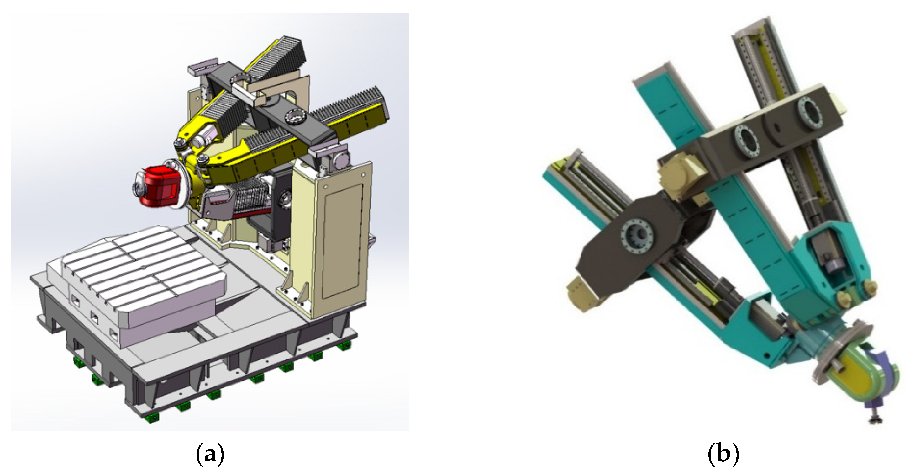
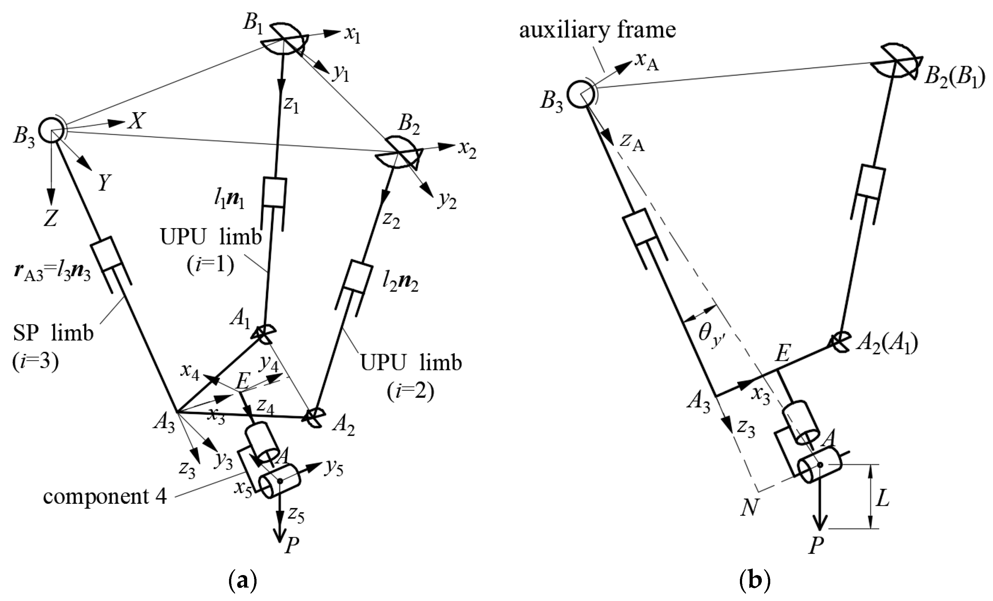
2.1. Structure Description

Figure 1 shows a 5-DOF hybrid robot that is used to machine aerospace structural components with composite material. It consists of a 2-DOF RR rotating head and a 3-DOF 2UPU/SP (where S represents spherical joints) parallel mechanism. The schematic diagram of the robot is shown in Figure 2. As shown in Figure 2a, the 2UPU/SP parallel mechanism consists of a fixed base, three limbs, and a moving platform (MP). Limb 1 and limb 2 are driven by prismatic (P) joints and connected with the MP and the base through universal (U) joints. Limb 3 is driven by a prismatic joint and connected with the base through a spherical (S) joint. The MP is rigidly attached to limb 3. The 2-DOF RR rotating head consists of two rotating joints. As Figure 2 shows, component 4 in RR rotating head is attached to the MP through a rotating joint whose axis is parallel to limb 3. Component 5 in RR rotating head is connected to component 4 through a rotating joint whose axis is perpendicular to the axis of the previous rotating joint.

Figure 1. 5-DOF hybrid robot [38]: (a) 3D model of the hybrid robot; (b) 2UPU/SP-RR mechanism.

Figure 2. Schematic diagram of 2UPU/SP-RR hybrid robot: (a) schematic diagram of the hybrid robot; (b) auxiliary frame.

As Figure 2a shows, B_i (i = 1, 2) denotes the center of the U joints attached to the base, B₃ denotes the center of the S joint, and A_i (i = 1, 2) denotes the center of the U joints connecting the MP. A₃ denotes the intersection of the SP limb and the plane where A_i (i = 1, 2) are located and SP limb is perpendicular to the plane determined by A_i (i = 1, 2, 3). Triangles ∆A₁A₂A₃ and ∆B₁B₂B₃ are isosceles and similar. In the rotating head, E represents the intersection of the axis of the first rotating joint of the rotating head and the plane spanned by A_i (i = 1, 2, 3), A represents the intersection of the two rotating axes of the rotating head and P represents the end point of end-effector. Fixed frame B₃-XYZ is established at point B₃ with the Y axis parallel to the line $B_1{B}_2$ and X axis pointing to the midpoint of the line $B_1{B}_2$. Besides, body fixed frame B_i-x_iy_iz_i (i = 1, 2), A₃-x₃y₃z₃, E-x₄y₄z₄ and A-x₅y₅z₅ are established. Frame B_i-x_iy_iz_i (i = 1, 2) is attached to point B_i with z_i axis pointing from B_i to A_i and y_i axis coincident with the first axis of the U joint. Frame A₃-x₃y₃z₃ is established at A₃ with z₃ axis coincident with the line $B_3{A}_3$ and x₃ axis pointing to the midpoint of the line A₁A₂. In E-x₄y₄z₄, y₄ axis is parallel to the axis of the second rotating joint of the rotating head, and z₄ axis is coincident with the line EA. In A-x₅y₅z₅, the z₅ axis points from A to P, and the y₅ axis coincides with the axis of the second joint of the rotating head. In addition, the axes not mentioned in the aforementioned frames satisfy the right-hand rule.

2.2. Inverse Position Analysis

2.2.1. Position Analysis of the Parallel Mechanism

For the inverse kinematics of the 5-DOF hybrid robot, the position and posture of the end-effector are given. The position vector of the end point can be represented by ${\mathit{r}}_P=(\begin{array}{ccc}{x}_p& y_p& z_p{)}^{\mathrm{T}}\end{array}$ and the posture of the end-effector can be expressed by two rotation angles α and β. The position vector of A, which is denoted by ${\mathit{r}}_A=(\begin{array}{ccc}{x}_A& y_A& z_A{)}^{\mathrm{T}}\end{array}$, can be obtained as

$${\mathit{r}}_A={\mathit{r}}_P-L{\mathit{n}}_P$$

(1)

where L represents the distance from points A to P, ${\mathit{n}}_P$ is the orientation vector of the end-effector and ${\mathit{n}}_P={\left[\begin{array}{ccc}\sin \beta & -\sin \alpha \cos \beta & \cos \alpha \cos \beta \end{array}\right]}^{\mathrm{T}}$. According to the geometric relationship, the length of limb 3 can be written as

$$l_3=\sqrt{x_A{}^2+y_A{}^2+z_A{}^2-d^2}-k$$

(2)

where d represents the distance from point A₃ to E and k represents the distance from E to A.

As Figure 2b shows, an auxiliary frame B₃-x_Ay_Az_A is established with z_A axis pointing from B₃ to A, y_A axis parallel to the y₃ axis of A₃-x₃y₃z₃, and x_A axis satisfying the right-hand rule. The rotation matrix of auxiliary frame B₃-x_Ay_Az_A can be expressed by XYZ Euler angles: firstly rotate ${\theta }_{Ax}$ about X-axis of the local frame; secondly rotate ${\theta }_{Ay}$ about the Y-axis of the new frame; finally rotate ${\theta }_{Az}$ about the Z-axis of the new frame. Based on the B₃-x_Ay_Az_A, the rotation matrix of A₃-x₃y₃z₃ can be obtained by rotating ${\theta }_{y\prime }$ around the y_A axis as [38]

$${\mathit{R}}_3={\mathit{R}}_{{\theta }_{Ax}}{\mathit{R}}_{{\theta }_{Ay}}{\mathit{R}}_{{\theta }_{Az}}{\mathit{R}}_{{\theta }_{y\prime }}$$

(3)

where ${\mathit{R}}_{{\theta }_{Ax}}$ represents the rotation matrix of angle ${\theta }_{Ax}$. According to Figure 2b, ${\theta }_{y\prime }$ can be obtained as

$${\theta }_{y\prime }=\arcsin (\frac{-d}{l_A})$$

(4)

where $l_A=\sqrt{x_A{}^2+y_A{}^2+z_A{}^2}$. The position vector of point A can be written as

$${\mathit{r}}_A={\mathit{R}}_A{\left[\begin{array}{ccc}0& 0& l_A\end{array}\right]}^{\mathrm{T}}={\left[\begin{array}{ccc}{l}_A\sin {\theta }_{Ay}& -l_A\sin {\theta }_{Ax}\cos {\theta }_{Ay}& l_A\cos {\theta }_{Ax}\cos {\theta }_{Ay}\end{array}\right]}^{\mathrm{T}}$$

(5)

Based on Equation (5), the angles ${\theta }_{Ax}$ and ${\theta }_{Ay}$ can be expressed as

$${\theta }_{Ax}=\arctan \left(-\frac{y_A}{z_A}\right),{\theta }_{Ay}=\arcsin \left(\frac{x_A}{l_A}\right)$$

(6)

The angle θ_Az must satisfy the structural constraint of plane A₁A₂B₂B₁ [39]. The plane constraint can be expressed as

$$({\mathit{r}}_{A2}-{\mathit{r}}_{A1})\times ({\mathit{r}}_{B1}-{\mathit{r}}_{A1})\cdot ({\mathit{r}}_{B2}-{\mathit{r}}_{A1})=0$$

(7)

where ${\mathit{r}}_{A1}={\mathit{r}}_{A3}+{\mathit{R}}_3{\left[\begin{array}{ccc}{p}_2& -q_2& 0\end{array}\right]}^{\mathrm{T}}$, ${\mathit{r}}_{A2}={\mathit{r}}_{A3}+{\mathit{R}}_3{\left[\begin{array}{ccc}{p}_2& q_2& 0\end{array}\right]}^{\mathrm{T}}$, ${\mathit{r}}_{A3}={\mathit{R}}_3{\left[\begin{array}{ccc}0& 0& l_3\end{array}\right]}^{\mathrm{T}}$, ${\mathit{r}}_{B1}={\left[\begin{array}{ccc}{p}_1& -q_1& 0\end{array}\right]}^{\mathrm{T}}$, ${\mathit{r}}_{B2}={\left[\begin{array}{ccc}{p}_1& q_1& 0\end{array}\right]}^{\mathrm{T}}$, $p_1$ and $p_2$ are the height of the base side of ∆B₁B₂B₃ and ∆A₁A₂A₃, and q₁ and q₂ are the half of the base side of ∆B₁B₂B₃ and ∆A₁A₂A₃. Based on Equations (3), (4), (6) and (7), the following equation can be obtained

$$\begin{array}{l}{z}_A{l}_A(l_3{}^2+k{l}_3+p_{2}d-p_1{x}_A)\sin {\theta }_{Az}+y_A(p_1{l}_A{}^2-x_A{l}_3{}^2-k{x}_A{l}_3-p_{2}d{x}_A)\cos {\theta }_{Az}\\ =y_A{l}_{Ayz}(p_2{l}_3+p_{2}k-d{l}_3)\end{array}$$

(8)

where $l_{Ayz}=\sqrt{y_A{}^2+z_A{}^2}$. ${\theta }_{Az}$ can be determined by Equation (8)

$${\theta }_{Az}=\arcsin \left(\frac{h_3}{\sqrt{h_1{}^2+h_2{}^2}}\right)-\arctan \left(\frac{h_2}{h_1}\right)$$

(9)

where $h_1=z_A{l}_A(l_3{}^2+k{l}_3+p_{2}d-p_1{x}_A)$, $h_2=y_A(p_1{l}_A{}^2-x_A{l}_3{}^2-k{x}_A{l}_3-p_{2}d{x}_A)$, $h_3=y_A{l}_{Ayz}(p_2{l}_3+p_{2}k-d{l}_3)$.

The position vector of point A₃ can be expressed by

$${\mathit{r}}_{A3}={\mathit{R}}_3{\left[\begin{array}{ccc}0& 0& l_3\end{array}\right]}^{\mathrm{T}}$$

(10)

The closed-loop constraint equation of limbs 1 and 2 can be obtained as

$${\mathit{r}}_{A3}=b_i+l_i{\mathit{n}}_i-{\mathit{a}}_i,i=1,2$$

(11)

where n_i and l_i denote the unit vector and length of the limb i; b_i is the position vector of B_i; ${\mathit{a}}_i={\mathit{R}}_3{}^3\mathit{a}_i$ and ${}^3\mathit{a}_i$ is the position vector of A_i in A₃-x₃y₃z₃. Based on Equations (10) and (11), l_i and n_i can be written as

$$l_i=\left|{\mathit{r}}_{A3}-{\mathit{b}}_i+{\mathit{a}}_i\right|,{\mathit{n}}_i=({\mathit{r}}_{A3}-{\mathit{b}}_i+{\mathit{a}}_i)/l_i,i=1,2$$

(12)

For limbs 1 and 2, the rotation matrix of B_i-x_iy_iz_i can be described by two rotations: first rotate θ_iy about Y-axis of the local frame; then rotate θ_ix about the new X-axis. The rotation matrix of B_i-x_iy_iz_i (i = 1, 2) can be obtained as ${\mathit{R}}_i={\mathit{R}}_{{\theta }_{iy}}{\mathit{R}}_{{\theta }_{ix}}$. Then n_i can be also expressed as

$${\mathit{n}}_i={\mathit{R}}_i{\mathit{e}}_{3,3}={\left[\begin{array}{ccc}\sin {\theta }_{iy}\cos {\theta }_{ix}& -\sin {\theta }_{ix}& \cos {\theta }_{iy}\cos {\theta }_{ix}\end{array}\right]}^{\mathrm{T}}$$

(13)

where e_j,i denotes a j-dimensional column vector in which the i-th element is 1 and the other elements are 0. The angle θ_iy and θ_ix can be obtained by Equation (13) as

$${\theta }_{iy}=\arctan (\frac{n_{ix}}{n_{iz}}),{\theta }_{ix}=\arcsin (-n_{iy})$$

(14)

2.2.2. Position Analysis of the Rotating Head

For the serial rotating head, the angle of the first rotating joint is represented by φ_z, and the angle of the second rotating joint is denoted by φ_y. The orientation vector of the end-effector can be obtained as

$${\mathit{n}}_P={\mathit{R}}_3{\mathit{R}}_{{\phi }_z}{\mathit{R}}_{{\phi }_y}{\mathit{e}}_{3,3}$$

(15)

The joint angles of the rotating head can be obtained by Equation (15) as

$${\phi }_y=\pm \arccos \left(k_3\right)$$

(16)

$${\phi }_z=\arg \left(\frac{k_1}{\sin {\phi }_y}+j\frac{k_2}{\sin {\phi }_y}\right)$$

(17)

where $k_i=({\mathit{R}}_3{}^{\mathrm{T}}{\mathit{n}}_P)\cdot {\mathit{e}}_{3,i}={({\mathit{R}}_3{\mathit{e}}_{3,i})}^{\mathrm{T}}{\mathit{n}}_P(i=1,2,3)$, arg(z) represents the principal argument angle of the complex number z, and j is the imaginary unit. There are two solutions of φ_y of Equation (16), and the solution of φ_y is selected according to the motion trajectory.

2.3. Inverse Velocity Analysis

2.3.1. Velocity Analysis of the Parallel Mechanism

Based on the principle of angular velocity superposition and Equation (3), the angular velocity of limb 3 can be written as

$${\mathit{\omega }}_3={\mathit{e}}_{3,1}{\dot{\theta }}_{Ax}+{\mathit{R}}_{{\theta }_{Ax}}{\mathit{e}}_{3,2}{\dot{\theta }}_{Ay}+{\mathit{R}}_{{\theta }_{Ax}}{\mathit{R}}_{{\theta }_{Ay}}{\mathit{e}}_{3,3}{\dot{\theta }}_{Az}+{\mathit{R}}_{{\theta }_{Ax}}{\mathit{R}}_{{\theta }_{Ay}}{\mathit{R}}_{{\theta }_{Az}}{\mathit{e}}_{3,2}{\dot{\theta }}_{y\prime }={\mathit{J}}_{a3}{\dot{\mathit{\Theta }}}_3$$

(18)

where ${\dot{\mathit{\Theta }}}_3={[\begin{array}{cccc}{\dot{\theta }}_{Ax}& {\dot{\theta }}_{Ay}& {\dot{\theta }}_{Az}& {\dot{\theta }}_{yt}\end{array}]}^{\mathrm{T}}$, ${\mathit{J}}_{a3}={[\begin{array}{cccc}{\mathit{e}}_{3,1}& {\mathit{R}}_{{\theta }_{Ax}}{\mathit{e}}_{3,2}& {\mathit{R}}_{{\theta }_{Ax}}{\mathit{R}}_{{\theta }_{Ay}}{\mathit{e}}_{3,3}& {\mathit{R}}_{{\theta }_{Ax}}{\mathit{R}}_{{\theta }_{Ay}}{\mathit{R}}_{{\theta }_{Az}}{\mathit{e}}_{3,2}\end{array}]}^{\mathrm{T}}$. It can be seen from Equations (4) and (6) that the angles θ_Ax, θ_Ay and θ_y’ are functions of x_A, y_A and z_A. Taking the time derivative of Equations (4) and (6) yields

$${\dot{\theta }}_{y\prime }={\mathit{J}}_{{\theta }_{y\prime }}{\dot{\mathit{r}}}_A,{\dot{\theta }}_{Ax}={\mathit{J}}_{{\theta }_{Ax}}{\dot{\mathit{r}}}_A,{\dot{\theta }}_{Ay}={\mathit{J}}_{{\theta }_{Ay}}{\dot{\mathit{r}}}_A$$

(19)

where

$${\mathit{J}}_{{\theta }_{y\prime }}=\left[\begin{array}{ccc}\frac{\partial {\theta }_{y\prime }}{\partial x_A}& \frac{\partial {\theta }_{y\prime }}{\partial y_A}& \frac{\partial {\theta }_{y\prime }}{\partial z_A}\end{array}\right]=\left[\begin{array}{ccc}\frac{x_{A}d}{l_A{}^2\sqrt{l_A{}^2-d^2}}& \frac{y_{A}d}{l_A{}^2\sqrt{l_A{}^2-d^2}}& \frac{z_{A}d}{l_A{}^2\sqrt{l_A{}^2-d^2}}\end{array}\right]$$

${\mathit{J}}_{{\theta }_{Ax}}$ and ${\mathit{J}}_{{\theta }_{Ay}}$ are given in the Appendix A. It can be seen from Equations (2), (4), (8) and (9) that the angle θ_Az can be expressed as a function of h₁, h₂ and h₃; auxiliary variables h₁, h₂ and h₃ are functions of l_A, l₃, l_Ayz, x_A, y_A and z_A; l_A, l₃ and l_Ayz are functions of x_A, y_A and z_A. Taking time derivative of Equation (9) yields

$${\dot{\theta }}_{Az}={\mathit{J}}_{{\theta }_{Az}1}\mathit{h}={\mathit{J}}_{{\theta }_{Az}1}{\mathit{J}}_{{\theta }_{Az}2}{[{\dot{l}}_A{\dot{l}}_3{\dot{l}}_{Ayz}{\dot{x}}_A{\dot{y}}_A{\dot{z}}_A]}^T={\mathit{J}}_{{\theta }_{Az}}{\dot{\mathit{r}}}_A$$

(20)

where ${\mathit{J}}_{{\theta }_{Az}}={\mathit{J}}_{{\theta }_{Az}1}{\mathit{J}}_{{\theta }_{Az}2}{\mathit{J}}_{{\theta }_{Az}3}$, ${\mathit{J}}_{{\theta }_{Az}1}=\left[\begin{array}{ccc}\frac{\partial {\theta }_{Az}}{\partial h_1}& \frac{\partial {\theta }_{Az}}{\partial h_2}& \frac{\partial {\theta }_{Az}}{\partial h_2}\end{array}\right]$

$${\mathit{J}}_{{\theta }_{Az}2}=\left[\begin{array}{cccccc}\frac{\partial h_1}{\partial l_A}& \frac{\partial h_1}{\partial l_3}& \frac{\partial h_1}{\partial l_{Ayz}}& \frac{\partial h_1}{\partial x_A}& \frac{\partial h_1}{\partial y_A}& \frac{\partial h_1}{\partial z_A}\\ \frac{\partial h_2}{\partial l_A}& \frac{\partial h_2}{\partial l_3}& \frac{\partial h_2}{\partial l_{Ayz}}& \frac{\partial h_2}{\partial x_A}& \frac{\partial h_2}{\partial y_A}& \frac{\partial h_2}{\partial z_A}\\ \frac{\partial h_3}{\partial l_A}& \frac{\partial h_3}{\partial l_3}& \frac{\partial h_3}{\partial l_{Ayz}}& \frac{\partial h_3}{\partial x_A}& \frac{\partial h_3}{\partial y_A}& \frac{\partial h_3}{\partial z_A}\end{array}\right],{\mathit{J}}_{{\theta }_{Az}3}=\left[\begin{array}{c}\begin{array}{ccc}\frac{\partial l_A}{\partial x_A}& \frac{\partial l_A}{\partial y_A}& \frac{\partial l_A}{\partial z_A}\\ \frac{\partial l_3}{\partial x_A}& \frac{\partial l_3}{\partial y_A}& \frac{\partial l_3}{\partial z_A}\\ \frac{\partial l_{Ayz}}{\partial x_A}& \frac{\partial l_{Ayz}}{\partial y_A}& \frac{\partial l_{Ayz}}{\partial z_A}\end{array}\\ E_{3\times 3}\end{array}\right]$$

${\mathit{J}}_{{\theta }_{Az}1}$, ${\mathit{J}}_{{\theta }_{Az}2}$ and ${\mathit{J}}_{{\theta }_{Az}3}$ are given in the Appendix A. ${\mathit{e}}_{3\times 3}$ represents a 3 × 3 identity matrix.

According to Equations (1) and (18)–(20), the angle velocity of limb 3 can be rewritten as

$${\mathit{\omega }}_3={\mathit{J}}_{a3}{\mathit{J}}_{\theta 3}{\dot{\mathit{r}}}_A={\mathit{J}}_{\omega 3}\dot{\mathit{X}}$$

(21)

where ${\mathit{J}}_{\omega 3}={\mathit{J}}_{a3}{\mathit{J}}_{\theta 3}{\mathit{J}}_{AX}$, ${\mathit{J}}_{\theta 3}={[\begin{array}{cccc}{\mathit{J}}_{{\theta }_{Ax}}{}^{\mathrm{T}}& {\mathit{J}}_{{\theta }_{Ay}}{}^{\mathrm{T}}& {\mathit{J}}_{{\theta }_{Az}}{}^{\mathrm{T}}& {\mathit{J}}_{{\theta }_{y\prime }}{}^{\mathrm{T}}\end{array}]}^{\mathrm{T}}$, ${\mathit{J}}_{AX}={\mathit{J}}_P-L{\mathit{J}}_{np}$, ${\mathit{J}}_P=[\begin{array}{cc}{\mathit{E}}_{3\times 3}& 0_{3\times 2}\end{array}]$, $0_{3\times 2}$ is a 3 × 2 null matrix, $\dot{\mathit{X}}={[\begin{array}{ccccc}{\dot{x}}_P& {\dot{y}}_P& {\dot{z}}_P& \dot{\alpha }& \dot{\beta }\end{array}]}^{\mathrm{T}}$ and ${\mathit{J}}_{np}=\left[\begin{array}{ccccc}0& 0& 0& 0& \cos \beta \\ 0& 0& 0& -\cos \alpha \cos \beta & \sin \alpha \sin \beta \\ 0& 0& 0& -\sin \alpha \cos \beta & -\cos \alpha \sin \beta \end{array}\right]$.

Taking time derivative of Equation (10) yields

$${\dot{\mathit{r}}}_{A3}={\mathit{\omega }}_3\times ({\mathit{R}}_3{\mathit{e}}_{3,3}{l}_3)+{\mathit{R}}_3{\mathit{e}}_{3,3}{\dot{l}}_3={\mathit{J}}_{A3}\dot{\mathit{X}}$$

(22)

where ${\mathit{J}}_{A3}=-[({\mathit{R}}_3{\mathit{e}}_{3,3}{l}_3)\times ]{\mathit{J}}_{\omega 3}+{\mathit{R}}_3{\mathit{e}}_{3,3}{\mathit{J}}_3{\mathit{J}}_{AX}$, ${\mathit{J}}_3$ is the third row of ${\mathit{J}}_{{\theta }_{Az}3}$ and $[({\mathit{R}}_3{\mathit{e}}_{3,3}{l}_3)\times ]$ represents the skew-symmetric matrix of vector ${\mathit{R}}_3{\mathit{e}}_{3,3}{l}_3$. For example, for a vector $\mathit{w}={[\begin{array}{ccc}{w}_x& w_y& w_z\end{array}]}^{\mathrm{T}}$, its skew-symmetric matrix is defined as $[\mathit{w}\times ]=\left[\begin{array}{ccc}0& -w_z& w_y\\ w_z& 0& -w_x\\ -w_y& w_x& 0\end{array}\right]$.

Taking the time derivative of Equation (11) leads to

$${\dot{\mathit{r}}}_{A3}={\dot{l}}_i{\mathit{n}}_i+l_i{\dot{\mathit{n}}}_i-{\mathit{\omega }}_3\times {\mathit{a}}_i,i=1,2$$

(23)

Because n_i is a unit vector, ${\dot{\mathit{n}}}_i\cdot {\mathit{n}}_i=0$. Taking the dot product with n_i on both sides of Equation (23) yields

$${\dot{l}}_i={\mathit{n}}_i{}^{\mathrm{T}}{\dot{\mathit{r}}}_{A3}+{({\mathit{a}}_i\times {\mathit{n}}_i)}^{\mathrm{T}}{\mathit{\omega }}_3,i=1,2$$

(24)

Rewriting ${\dot{l}}_i(i=1,2,3)$ in matrix form leads to

$$\dot{\mathit{l}}={\mathit{J}}_l\dot{X}$$

(25)

where $\dot{\mathit{l}}={[\begin{array}{ccc}{\dot{l}}_1& {\dot{l}}_2& {\dot{l}}_3\end{array}]}^{\mathrm{T}}$, ${\mathit{J}}_l={[\begin{array}{ccc}{({\mathit{n}}_1{}^{\mathrm{T}}{\mathit{J}}_{A3}+{({\mathit{a}}_1\times {\mathit{n}}_1)}^{\mathrm{T}}{\mathit{J}}_{\omega 3})}^{\mathrm{T}}& {({\mathit{n}}_2{}^{\mathrm{T}}{\mathit{J}}_{A3}+{({\mathit{a}}_2\times {\mathit{n}}_2)}^{\mathrm{T}}{\mathit{J}}_{\omega 3})}^{\mathrm{T}}& {({\mathit{J}}_3{\mathit{J}}_{AX})}^{\mathrm{T}}\end{array}]}^{\mathrm{T}}$.

According to Equations (14) and (23) and the principle of angular velocity superposition, the angular velocity of limb i (i = 1, 2) is given by

$${\mathit{\omega }}_i={\mathit{e}}_{3,2}{\dot{\theta }}_{iy}+{\mathit{R}}_{{\theta }_{iy}}{\mathit{e}}_{3,1}{\dot{\theta }}_{ix}={\mathit{J}}_{ai}{\dot{\mathit{\Theta }}}_i={\mathit{J}}_{ai}{\mathit{J}}_{\theta i}{\dot{\mathit{n}}}_i={\mathit{J}}_{\omega i}\dot{X}$$

(26)

where ${\mathit{J}}_{\omega i}={\mathit{J}}_{ai}{\mathit{J}}_{\theta i}{\mathit{J}}_{ni}$, ${\mathit{J}}_{ni}=({\mathit{J}}_{A3}-{\mathit{n}}_i{\mathit{J}}_{li}-[{\mathit{a}}_i\times ]{\mathit{J}}_{\omega 3})/l_i$, ${\mathit{J}}_{li}$ is the i-th row of ${\mathit{J}}_l$, ${\mathit{J}}_{ai}=[\begin{array}{cc}{\mathit{e}}_{3,2}& {\mathit{R}}_{{\theta }_{iy}}{\mathit{e}}_{3,1}\end{array}]$, ${\dot{\mathit{\Theta }}}_i={[\begin{array}{cc}{\dot{\theta }}_{iy}& {\dot{\theta }}_{ix}\end{array}]}^{\mathrm{T}}$ and

$${\mathit{J}}_{\theta i}=\left[\begin{array}{ccc}\frac{n_{iz}}{n_{ix}{}^2+n_{iz}{}^2}& 0& \frac{-n_{ix}}{n_{ix}{}^2+n_{iz}{}^2}\\ 0& \frac{-1}{\sqrt{1-n_{iy}{}^2}}& 0\end{array}\right]$$

2.3.2. Velocity Analysis of the Rotating Head

Taking time derivative of Equations (16) and (17) yields

$$\dot{\mathit{\Phi }}={[\begin{array}{cc}{\dot{\phi }}_z& {\dot{\phi }}_y\end{array}]}^{\mathrm{T}}={\mathit{J}}_m\dot{\mathit{k}}={\mathit{J}}_{\phi }\dot{\mathit{X}}$$

(27)

where $\dot{\mathit{k}}={[\begin{array}{ccc}{\dot{k}}_1& {\dot{k}}_2& {\dot{k}}_3\end{array}]}^{\mathrm{T}}$ and ${\mathit{J}}_{\phi }={\mathit{J}}_m{\mathit{J}}_k$. The i-th (i = 1, 2, 3) row of ${\mathit{J}}_k$ can be written as ${(({\mathit{R}}_3{\mathit{e}}_{3,i})\times {\mathit{n}}_P)}^{\mathrm{T}}{\mathit{J}}_{\omega 3}+{({\mathit{R}}_3{\mathit{e}}_{3,i})}^{\mathrm{T}}{\mathit{J}}_{np}$. When ${\phi }_y=\arccos \left(k_3\right)$, ${\mathit{J}}_m$ can be expressed as

$${\mathit{J}}_m=\left[\begin{array}{ccc}\frac{-k_2}{k_1{}^2+k_2{}^2}& \frac{k_1}{k_1{}^2+k_2{}^2}& 0\\ 0& 0& -\frac{1}{\sqrt{1-k_3{}^2}}\end{array}\right]$$

When ${\phi }_y=-\arccos \left(k_3\right)$, the second row of ${\mathit{J}}_m$ becomes its opposite number.

According to the principle of angular velocity superposition, the angular velocity of component 4 can be obtained as

$${\mathit{\omega }}_4={\mathit{\omega }}_3+{\mathit{R}}_3{\mathit{e}}_{3,3}{\dot{\phi }}_z={\mathit{J}}_{\omega 4}\dot{\mathit{X}}$$

(28)

where ${\mathit{J}}_{\omega 4}={\mathit{J}}_{\omega 3}+{\mathit{R}}_3{\mathit{e}}_{3,3}{\mathit{e}}_{2,1}{}^{\mathrm{T}}{\mathit{J}}_{\phi }$. Similarly, the angular velocity of component 5 can be expressed as

$${\mathit{\omega }}_5={\mathit{\omega }}_4+{\mathit{R}}_4{\mathit{e}}_{3,2}{\dot{\phi }}_y={\mathit{J}}_{\omega 5}\dot{\mathit{X}}$$

(29)

where ${\mathit{J}}_{\omega 5}={\mathit{J}}_{\omega 4}+{\mathit{R}}_4{\mathit{e}}_{3,2}{\mathit{e}}_{2,2}{}^{\mathrm{T}}{\mathit{J}}_{\phi }$.

2.4. Inverse Acceleration Analysis

The angle acceleration of limb 3 can be obtained by taking time derivative of Equation (21) as

$${\dot{\mathit{\omega }}}_3={\mathit{J}}_{\omega 3}\ddot{\mathit{X}}+{\dot{\mathit{J}}}_{\omega 3}\dot{\mathit{X}}$$

(30)

where ${\dot{\mathit{J}}}_{\omega 3}={\dot{\mathit{J}}}_{a3}{\mathit{J}}_{\theta 3}{\mathit{J}}_{AX}+{\mathit{J}}_{a3}{\dot{\mathit{J}}}_{\theta 3}{\mathit{J}}_{AX}+{\mathit{J}}_{a3}{\mathit{J}}_{\theta 3}{\dot{\mathit{J}}}_{AX}$. Equation (18) shows that the elements in ${\mathit{J}}_{a3}$ are functions of θ_Ax, θ_Ay and θ_Az. Thus, the elements of the i-th row and j-th column in ${\mathit{J}}_{a3}$ can be expressed as

$$a_{i,j}=a_{i,j}({\theta }_{Ax},{\theta }_{Ay},{\theta }_{Az})$$

(31)

The elements of the i-th row and j-th column in ${\dot{\mathit{J}}}_{a3}$ can be written as

$${\dot{a}}_{i,j}=\frac{\partial a_{i,j}}{\partial {\theta }_{Ax}}{\dot{\theta }}_{Ax}+\frac{\partial a_{i,j}}{\partial {\theta }_{Ay}}{\dot{\theta }}_{Ay}+\frac{\partial a_{i,j}}{\partial {\theta }_{Az}}{\dot{\theta }}_{Az}$$

(32)

${\dot{\mathit{J}}}_{a3}$ can be obtained by Matlab software developed by MathWorks, Inc., the United States. ${\dot{\mathit{J}}}_{\theta 3}$ and ${\dot{\mathit{J}}}_{AX}$ can be obtained through a similar method.

Taking the time derivative of Equation (25) leads to

$$\dot{\mathit{l}}={\mathit{J}}_l\ddot{\mathit{X}}+{\dot{\mathit{J}}}_l\dot{\mathit{X}}$$

(33)

where

$${\dot{\mathit{J}}}_l=\left[\begin{array}{c}{({\mathit{\omega }}_1\times {\mathit{n}}_1)}^{\mathrm{T}}{\mathit{J}}_{A3}+{\mathit{n}}_1{}^{\mathrm{T}}{\dot{\mathit{J}}}_{A3}+{(({\mathit{\omega }}_3\times {\mathit{a}}_1)\times {\mathit{n}}_1)}^{\mathrm{T}}{\mathit{J}}_{\omega 3}+{({\mathit{a}}_1\times ({\mathit{\omega }}_1\times {\mathit{n}}_1))}^{\mathrm{T}}{\mathit{J}}_{\omega 3}+{({\mathit{a}}_1\times {\mathit{n}}_1)}^{\mathrm{T}}{\dot{\mathit{J}}}_{\omega 3}\\ {({\mathit{\omega }}_2\times {\mathit{n}}_2)}^{\mathrm{T}}{\mathit{J}}_{A3}+{\mathit{n}}_2{}^{\mathrm{T}}{\dot{\mathit{J}}}_{A3}+{(({\mathit{\omega }}_3\times {\mathit{a}}_2)\times {\mathit{n}}_2)}^{\mathrm{T}}{\mathit{J}}_{\omega 3}+{({\mathit{a}}_2\times ({\mathit{\omega }}_2\times {\mathit{n}}_2))}^{\mathrm{T}}{\mathit{J}}_{\omega 3}+{({\mathit{a}}_2\times {\mathit{n}}_2)}^{\mathrm{T}}{\dot{\mathit{J}}}_{\omega 3}\\ {\dot{\mathit{J}}}_3{\mathit{J}}_{AX}+{\mathit{J}}_3{\dot{\mathit{J}}}_{AX}\end{array}\right]$$

$$\begin{array}{l}{\dot{\mathit{J}}}_{A3}=-[({\mathit{\omega }}_3\times {\mathit{R}}_3{\mathit{E}}_{3,3}{l}_3)\times ]{\mathit{J}}_{\omega 3}-[({\mathit{R}}_3{\mathit{E}}_{3,3}{\dot{l}}_3)\times ]{\mathit{J}}_{\omega 3}-[({\mathit{R}}_3{\mathit{E}}_{3,3}{l}_3)\times ]{\dot{\mathit{J}}}_{\omega 3}\\ +({\mathit{\omega }}_3\times {\mathit{R}}_3{\mathit{E}}_{3,3}){\mathit{J}}_3{\mathit{J}}_{AX}+{\mathit{R}}_3{\mathit{E}}_{3,3}{\dot{\mathit{J}}}_3{\mathit{J}}_{AX}+{\mathit{R}}_3{\mathit{E}}_{3,3}{\mathit{J}}_3{\dot{\mathit{J}}}_{AX}\end{array}$$

Differentiating Equation (26) with respect to time leads to

$${\dot{\omega }}_i={\mathit{J}}_{\omega i}\ddot{\mathit{X}}+{\dot{\mathit{J}}}_{\omega i}\dot{\mathit{X}}$$

(34)

where ${\dot{\mathit{J}}}_{\omega i}={\dot{\mathit{J}}}_{ai}{\mathit{J}}_{\theta i}{\mathit{J}}_{ni}+{\mathit{J}}_{ai}{\dot{\mathit{J}}}_{\theta i}{\mathit{J}}_{ni}+{\mathit{J}}_{ai}{\mathit{J}}_{\theta i}{\dot{\mathit{J}}}_{ni}$

• ${\dot{\mathit{J}}}_{ni}=({\dot{\mathit{J}}}_{A3}-({\mathit{\omega }}_i\times {\mathit{n}}_i){\mathit{J}}_{li}-{\mathit{n}}_i{\dot{\mathit{J}}}_{li}-[({\mathit{\omega }}_3\times {\mathit{a}}_i)\times ]{\mathit{J}}_{\omega 3}-[{\mathit{a}}_i\times ]{\dot{\mathit{J}}}_{\omega 3}-{\dot{l}}_i{\mathit{J}}_{ni})/l_i$

${\dot{\mathit{J}}}_{ai}$ and ${\dot{\mathit{J}}}_{\theta i}$ can be obtained by a similar method of solving ${\dot{\mathit{J}}}_{a3}$.

Taking the time derivative of Equation (28) yields

$${\dot{\mathit{\omega }}}_4={\mathit{J}}_{\omega 4}\ddot{\mathit{X}}+{\dot{\mathit{J}}}_{\omega 4}\dot{\mathit{X}}$$

(35)

where ${\dot{\mathit{J}}}_{\omega 4}={\dot{\mathit{J}}}_{\omega 3}+({\mathit{\omega }}_3\times {\mathit{R}}_3{\mathit{e}}_{3,3}){\mathit{e}}_{2,1}{}^{\mathrm{T}}{\mathit{J}}_{\phi }+{\mathit{R}}_3{\mathit{e}}_{3,3}{\mathit{e}}_{2,1}{}^{\mathrm{T}}{\dot{\mathit{J}}}_{\phi }$ and ${\dot{\mathit{J}}}_{\phi }={\dot{\mathit{J}}}_m{\mathit{J}}_k+{\mathit{J}}_m{\dot{\mathit{J}}}_k$. ${\dot{\mathit{J}}}_m$ can be obtained by a similar method of solving ${\dot{\mathit{J}}}_{a3}$. The i-th (i = 1, 2, 3) row of ${\dot{\mathit{J}}}_k$ can be obtained as

$$\begin{array}{ll}{\dot{J}}_{ki}=& {(({\mathit{\omega }}_3\times {\mathit{R}}_3{\mathit{e}}_{3,i})\times {\mathit{n}}_P)}^{\mathrm{T}}{\mathit{J}}_{\omega 3}+{(({\mathit{R}}_3{\mathit{e}}_{3,i})\times {\dot{\mathit{n}}}_P)}^{\mathrm{T}}{\mathit{J}}_{\omega 3}+{(({\mathit{R}}_3{\mathit{e}}_{3,i})\times {\mathit{n}}_P)}^{\mathrm{T}}{\dot{\mathit{J}}}_{\omega 3}\\ & +{({\mathit{\omega }}_3\times {\mathit{R}}_3{\mathit{e}}_{3,i})}^{\mathrm{T}}{\mathit{J}}_{np}+{({\mathit{R}}_3{\mathit{e}}_{3,i})}^{\mathrm{T}}{\dot{\mathit{J}}}_{np}\end{array}$$

Taking the time derivative of Equation (29) leads to

$${\dot{\mathit{\omega }}}_5={\mathit{J}}_{\omega 5}\ddot{\mathit{X}}+{\dot{\mathit{J}}}_{\omega 5}\dot{\mathit{X}}$$

(36)

where ${\dot{\mathit{J}}}_{\omega 5}={\dot{\mathit{J}}}_{\omega 4}+({\mathit{\omega }}_4\times {\mathit{R}}_4{\mathit{e}}_{3,2}){\mathit{e}}_{2,2}{}^{\mathrm{T}}{\mathit{J}}_{\phi }+{\mathit{R}}_4{\mathit{e}}_{3,2}{\mathit{e}}_{2,2}{}^{\mathrm{T}}{\dot{\mathit{J}}}_{\phi }$.

3. Inverse Dynamic Analysis

The inverse dynamics is to determine the driving force or driving torque with a given motion and external force of the end-effector. To simplify the analysis, the joint inertia is neglected. As Figure 3 shows, the limb of the parallel mechanism can be divided into two components according to the nature of motion. The motion of the first component S_i1 including the limb body, linear guideway, and motor is a general motion. The motion of the second component S_i2 including the lead-screw, coupler, and motor rotor is the afore-mentioned motion plus a rotation about the n_i axis. The virtual power of limb i can be obtained as

$$\begin{array}{ll}\delta P_i=& \delta {\dot{\mathit{r}}}_{Ci}{}^{\mathrm{T}}(m_i\mathit{g}-m_i{\ddot{\mathit{r}}}_{Ci})+\delta {\mathit{\omega }}_i{}^{\mathrm{T}}(-{\mathit{I}}_i{\dot{\mathit{\omega }}}_i-{\mathit{\omega }}_i\times ({\mathit{I}}_i{\mathit{\omega }}_i))\\ & +\delta {\mathit{\omega }}_{mi}{}^{\mathrm{T}}(-{\mathit{I}}_{mi}{\dot{\mathit{\omega }}}_{mi}-{\mathit{\omega }}_{mi}\times ({\mathit{I}}_{mi}{\mathit{\omega }}_{mi})),i=1,2,3\end{array}$$

(37)

where ${\mathit{I}}_i={\mathit{R}}_i\mathit{I}{\prime }_i{\mathit{R}}_i{}^{\mathrm{T}}$ and $\mathit{I}{\prime }_i$ is the inertia matrix of S_i1 with respect to the centroid; ${\mathit{I}}_{mi}={\mathit{R}}_i\mathit{I}{\prime }_{mi}{\mathit{R}}_i{}^{\mathrm{T}}$ and $\mathit{I}{\prime }_{mi}$ is the inertia matrix of S_i2 with respect to the centroid; g represents the gravitational acceleration; m_i represents the mass of S_i1 and S_i2 as a whole; ${\dot{\mathit{r}}}_{Ci}$ and ${\ddot{\mathit{r}}}_{Ci}$ are the velocity and acceleration of the centroid of limb i which is denoted by C_i; ${\mathit{\omega }}_{mi}$ and ${\dot{\omega }}_{mi}$ represent the angular velocity and acceleration of S_i2. According to Figure 3, we can obtain

$${\mathit{r}}_{C3}=(l_3-e_3){\mathit{n}}_3,{\mathit{r}}_{Ci}={\mathit{b}}_i+(l_i-e_i){\mathit{n}}_i,i=1,2$$

(38)

$${\dot{\mathit{r}}}_{Ci}={\mathit{J}}_{vci}\dot{\mathit{X}},i=1,2,3$$

(39)

$${\ddot{\mathit{r}}}_{Ci}={\mathit{J}}_{vci}\ddot{\mathit{X}}+{\dot{\mathit{J}}}_{vci}\dot{\mathit{X}},i=1,2,3$$

(40)

where ${\mathit{J}}_{vci}={\mathit{n}}_i{\mathit{J}}_{li}-(l_i-e_i)[{\mathit{n}}_i\times ]{\mathit{J}}_{\omega i}$, ${\mathit{J}}_{li}$ represents the i-th row of ${\mathit{J}}_l$, e_i is the distance from A_i to C_i, ${\dot{\mathit{J}}}_{vci}=({\mathit{\omega }}_i\times {\mathit{n}}_i){\mathit{J}}_{li}+{\mathit{n}}_i{\dot{\mathit{J}}}_{li}-{\dot{l}}_i[{\mathit{n}}_i\times ]{\mathit{J}}_{\omega i}-(l_i-e_i)([({\mathit{\omega }}_i\times {\mathit{n}}_i)\times ]{\mathit{J}}_{\omega i}+[{\mathit{n}}_i\times ]{\dot{\mathit{J}}}_{\omega i})$ and ${\dot{\mathit{J}}}_{li}$ is the i-th row of ${\dot{\mathit{J}}}_l$. The angular velocity of S_i2 in B₃-XYZ can be obtained as

$${\mathit{\omega }}_{mi}={\mathit{\omega }}_i+\frac{2\pi {\dot{l}}_i}{p_i}{\mathit{n}}_i={\mathit{J}}_{\omega mi}{\dot{\mathit{r}}}_3,{\mathit{J}}_{\omega mi}={\mathit{J}}_{\omega i}+\frac{2\pi {\mathit{n}}_i{\mathit{J}}_{li}}{p_i}$$

(41)

where p_i is the pitch of the lead-screw. The angular acceleration of S_i2 can be obtained by Differentiating Equation (41) with respect to time as

$${\dot{\mathit{\omega }}}_{mi}={\mathit{J}}_{\omega mi}{\ddot{\mathit{r}}}_3+{\dot{\mathit{J}}}_{\omega mi}{\dot{\mathit{r}}}_3$$

(42)

where ${\dot{\mathit{J}}}_{\omega mi}={\dot{\mathit{J}}}_{\omega i}+\frac{2\pi ({\mathit{\omega }}_i\times {\mathit{n}}_i){\mathit{J}}_{li}}{p_i}+\frac{2\pi {\mathit{n}}_i{\dot{\mathit{J}}}_{li}}{p_i}$.

The virtual power of the components of the rotating head can be expressed as

$$\delta P_i=\delta {\dot{\mathit{r}}}_{Ci}{}^{\mathrm{T}}(m_i\mathit{g}-m_i{\ddot{\mathit{r}}}_{Ci})+\delta {\mathit{\omega }}_i{}^{\mathrm{T}}(-{\mathit{I}}_i{\dot{\mathit{\omega }}}_i-{\mathit{\omega }}_i\times ({\mathit{I}}_i{\mathit{\omega }}_i)),i=4,5$$

(43)

where m_i is the mass of component i; ${\mathit{I}}_i={\mathit{R}}_i\mathit{I}{\prime }_i{\mathit{R}}_i{}^{\mathrm{T}}$ and $\mathit{I}{\prime }_i$ is the inertia matrix of component i with respect to the centroid; ${\dot{\mathit{r}}}_{Ci}$ and ${\ddot{\mathit{r}}}_{Ci}$ are the velocity and acceleration of the centroid of component i. According to Figure 2, we can obtain

$${\mathit{r}}_{C4}={\mathit{r}}_{A3}+{\mathit{R}}_3{}^3\mathit{r}_{C4},{\mathit{r}}_{C5}={\mathit{r}}_A+{\mathit{R}}_5{}^5\mathit{r}_{C5}$$

(44)

$${\dot{\mathit{r}}}_{Ci}={\mathit{J}}_{vci}\dot{\mathit{X}},i=4,5$$

(45)

$${\ddot{\mathit{r}}}_{Ci}={\mathit{J}}_{vci}\ddot{\mathit{X}}+{\dot{\mathit{J}}}_{vci}\dot{\mathit{X}},i=4,5$$

(46)

where ${\mathit{J}}_{vc4}={\mathit{J}}_{A3}-[({\mathit{R}}_3{}^3\mathit{r}_{C4})\times ]{\mathit{J}}_{\omega 3}$

• ${\mathit{J}}_{vc5}={\mathit{J}}_{AX}-[({\mathit{R}}_5{}^5\mathit{r}_{C5})\times ]{\mathit{J}}_{\omega 5}$
• ${\dot{\mathit{J}}}_{vc4}={\dot{\mathit{J}}}_{A3}-[({\mathit{\omega }}_3\times {\mathit{R}}_3{}^3\mathit{r}_{C4})\times ]{\mathit{J}}_{\omega 3}-[({\mathit{R}}_3{}^3\mathit{r}_{C4})\times ]{\dot{\mathit{J}}}_{\omega 3}$
• ${\dot{\mathit{J}}}_{vc5}={\dot{\mathit{J}}}_{AX}-[({\mathit{\omega }}_5\times {\mathit{R}}_5{}^5\mathit{r}_{C5})\times ]{\mathit{J}}_{\omega 5}-[({\mathit{R}}_5{}^5\mathit{r}_{C5})\times ]{\dot{\mathit{J}}}_{\omega 5}$

${}^3\mathit{r}_{C4}$ denotes the position vector of C₄ in A₃-x₃y₃z₃ and ${}^5\mathit{r}_{C5}$ is the position vector of C₅ in A-x₅y₅z₅.

The virtual work principle yields

$${\displaystyle \sum _{i=1}^5\delta P_i}+\delta {\dot{\mathit{q}}}^{\mathrm{T}}\mathit{f}+\delta {\dot{\mathit{r}}}_P{}^{\mathrm{T}}\mathit{F}+\delta {\mathit{\omega }}_5{}^{\mathrm{T}}\mathit{T}=0$$

(47)

where f = [f₁, f₂, f₃, τ₄, τ₅]^T represents the actuating force vector, T and F represent the external torque and external force on end-effector with respect to point P, $\delta \dot{\mathit{q}}={[\begin{array}{ccccc}{\dot{l}}_1& {\dot{l}}_2& {\dot{l}}_3& {\dot{\phi }}_z& {\dot{\phi }}_y\end{array}]}^{\mathrm{T}}$, $\delta \dot{\mathit{q}}={\mathit{J}}_q\delta \dot{\mathit{X}}$, ${\mathit{J}}_q={[\begin{array}{cc}{\mathit{J}}_l{}^{\mathrm{T}}& {\mathit{J}}_{\phi }{}^{\mathrm{T}}\end{array}]}^{\mathrm{T}}$, $\delta {\mathit{v}}_P={\mathit{J}}_{vp}\delta \dot{\mathit{X}}$ and ${\mathit{J}}_{vp}=[\begin{array}{cc}{\mathit{E}}_{3\times 3}& 0_{3\times 2}\end{array}]$. By substituting Equations (37) and (43) into Equation (47), the inverse dynamic equation of the hybrid robot can be written as

$$\mathit{f}={\mathit{f}}_a+{\mathit{f}}_v+{\mathit{f}}_g$$

(48)

where ${\mathit{f}}_a=\mathit{M}(\mathit{X})\ddot{\mathit{X}}$ represents the acceleration term, ${\mathit{f}}_v=\mathit{C}(\mathit{X},\dot{\mathit{X}})\dot{\mathit{X}}$ represents the velocity term, ${\mathit{f}}_g=\mathit{G}(\mathit{X})$ represents the gravity and external force term,

$$\begin{gathered} \mathit{M}={\mathit{J}}_q{}^{-\mathrm{T}}\left[{\displaystyle \sum _{i=1}^5\left(m_i{\mathit{J}}_{vci}{}^{\mathrm{T}}{\mathit{J}}_{vci}+{\mathit{J}}_{\omega i}{}^{\mathrm{T}}{\mathit{I}}_i{\mathit{J}}_{\omega i}\right)}+{\displaystyle \sum _{i=1}^3\left({\mathit{J}}_{\omega mi}{}^{\mathrm{T}}{\mathit{I}}_{mi}{\mathit{J}}_{\omega mi}\right)}\right] \\ \mathit{C}={\mathit{J}}_q{}^{-\mathrm{T}}\left[\begin{array}{l}{\displaystyle \sum _{i=1}^5\left(m_i{\mathit{J}}_{vci}{}^{\mathrm{T}}{\dot{\mathit{J}}}_{vci}+{\mathit{J}}_{\omega i}{}^{\mathrm{T}}{\mathit{I}}_i{\dot{\mathit{J}}}_{\omega i}-{\mathit{J}}_{\omega i}{}^{\mathrm{T}}\left[\left({\mathit{I}}_i{\mathit{\omega }}_i\right)\times \right]{\mathit{J}}_{\omega i}\right)}\\ +{\displaystyle \sum _{i=1}^3\left({\mathit{J}}_{\omega mi}{}^{\mathrm{T}}{\mathit{I}}_{mi}{\dot{\mathit{J}}}_{\omega mi}-{\mathit{J}}_{\omega mi}{}^{\mathrm{T}}\left[\left({\mathit{I}}_{mi}{\mathit{\omega }}_{mi}\right)\times \right]{\mathit{J}}_{\omega mi}\right)}\end{array}\right] \\ \mathit{G}=-{\mathit{J}}_q{}^{-\mathrm{T}}\left({\displaystyle \sum _{i=1}^5{m}_i{\mathit{J}}_{vci}{}^{\mathrm{T}}\mathit{g}}+{\mathit{J}}_{vp}{}^{\mathrm{T}}\mathit{F}+{\mathit{J}}_{\omega 5}{}^{\mathrm{T}}\mathit{T}\right) \end{gathered}$$

Figure 3. Schematic diagrams of limb structure. Reprinted with permission from ref. [40]. Copyright 2021 Elsevier.

4. Dynamic Performance Evaluation

4.1. Dynamic Performance Indices

For the limbs of the parallel mechanism, for given acceleration and velocity range of the end-effector, the driving force demand of each motor for a specific position and posture of end-effector can be written as

$$f_{i,\min }(\mathit{X})\le f_i\le f_{i,\max }(\mathit{X}),i=1,2,3$$

(49)

where $f_{i,\min }$ and $f_{i,\max }$ are the minimum and maximum of $f_i$ at the given position and posture. For the same motion of end-effector, a larger absolute value of driving force means higher requirements for the motor, and it will be more difficult to change the velocity and acceleration of end-effector. At the same time, the robot will bear greater internal force, which will have an adverse impact on the accuracy of the robot. Therefore, a larger absolute value of driving force can be considered as a worse working situation, and a local dynamic performance index can be defined as

$$f_{i\max }=\max \{\left|f_{i,\max }\right|,\left|f_{i,\min }\right|\}$$

(50)

Since the $f_{i\max }$ changes with the robot configuration, a global index to evaluate the average dynamic performance of the robot in the workspace can be defined as

$${\overline{f}}_{i\max }=\frac{{\displaystyle \underset{W_t}{\int }{f}_{i\max }dV}}{{\displaystyle \underset{W_t}{\int }dV}}$$

(51)

where W_t represents the workspace.

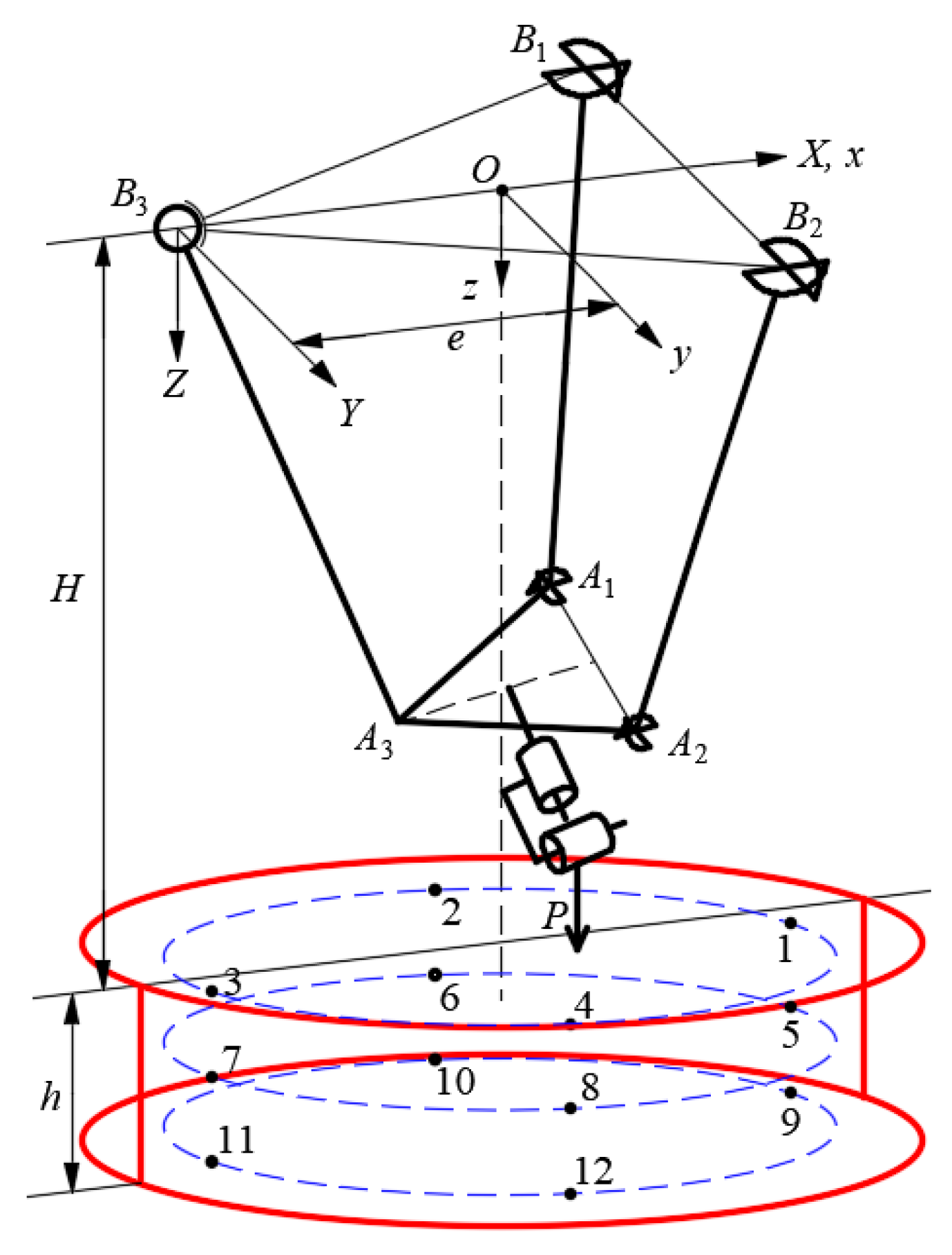
4.2. Task Space and Motion Range of the Hybrid Robot

As shown by the red line in Figure 4, the task workspace of the hybrid robot is a cylinder whose radius is 600 mm. h = 300 mm is the height of the workspace, H = 1650 mm is the distance from O to the upper bound of the workspace and e = 422.5 mm is the distance between the Y to y axes of O-xyz. According to the practical application requirements, the required range of the posture of end-effector is specified as $-20°\le \alpha \le 20°$ and $-20°\le \beta \le 20°$. To ensure that the robot is not singular in the workspace, we investigate the singularity of matrix M in Equation (48). The distribution of the minimum of determinant of matrix M under the required posture range in the lower layer where z = 1900 mm, middle layer where z = 1800 mm and upper layer where z = 1700 mm of the workspace is shown in Figure 5. It can be seen that the determinant of matrix M is far away from zero in the workspace, so matrix M is nonsingular in the workspace, which ensures the rationality of subsequent analysis.

Figure 4. Workspace of the hybrid robot and typical position in the workspace.

Figure 5. Distribution of minimum of determinant of matrix M under the required posture range in the workspace.

The 2UPU/SP-RR hybrid robot has three translational DOFs and two rotational DOFs. In order to calculate the maximum absolute value of driving force at a given position in the workspace, the posture of the end-effector is taken as the limiting condition, whose range is specified as $-20°\le \alpha \le 20°$ and $-20°\le \beta \le 20°$.

According to Equation (48), the driving force of limb i at a given position can be written as

$$f_i=f_{ai}(\ddot{x},\ddot{y},\ddot{z},\ddot{\alpha },\ddot{\beta },\alpha ,\beta )+f_{vi}(\dot{x},\dot{y},\dot{z},\dot{\alpha },\dot{\beta },\alpha ,\beta )+f_{gi}(\alpha ,\beta )$$

(52)

where $f_{ai}={\mathit{M}}_i\ddot{\mathit{X}}$, $f_{vi}={\mathit{C}}_i\dot{\mathit{X}}$, $f_{gi}=G_i$, and M_i, C_i and G_i are the i-th row of M, C and G.

It can be seen from Equation (52) that the acceleration term is determined by the acceleration and posture of the end-effector, the velocity term is determined by the velocity and posture of the end-effector, and the gravity and external force term is determined by posture. To simplify the calculation of the maximum absolute value of f_i, the influence of posture on the acceleration and velocity term is investigated. Twelve typical positions are selected on the circle with a radius of 500 mm in the lower layer, middle layer, and upper layer of the workspace, as shown in Figure 4. The distributions of maximum and minimum values of the acceleration and velocity term with posture at these typical positions are calculated by the MultiStart solver of Matlab 2016b. The ratio of the standard deviation to the mean value, which reflects the effect of the posture of the end-effector on the maximum and minimum acceleration and velocity term, is shown in Figure 6.

Figure 6. The influence of posture of end-effector on acceleration and velocity term: (a) influence on the maximum of acceleration and velocity term; (b) influence on the minimum of acceleration and velocity term.

Figure 6 shows that the posture of the end-effector has little effect on the maximums and minimums of acceleration and velocity items. In order to simplify the calculation, the effect of the posture of the end-effector is ignored to calculate the acceleration and velocity item, namely

$$f_i=f_{ai}(\ddot{x},\ddot{y},\ddot{z},\ddot{\alpha },\ddot{\beta })+f_{vi}(\dot{x},\dot{y},\dot{z},\dot{\alpha },\dot{\beta })+f_{gi}(\alpha ,\beta )$$

(53)

Then, we can obtain that

$$f_{i,\min }=f_{ai,\min }+f_{vi,\min }+f_{gi,\min },f_{i,\max }=f_{ai,\max }+f_{vi,\max }+f_{gi,\max }$$

(54)

According to the practical application requirements, the velocity and acceleration requirements of the hybrid robot are given as $\left|\ddot{x}\right|\le 2.5 \mathrm{m}/{\mathrm{s}}^2$, $\left|\dot{x}\right|\le 0.5 \mathrm{m}/\mathrm{s}$, $\left|\ddot{y}\right|\le 2.5 \mathrm{m}/{\mathrm{s}}^2$, $\left|\dot{y}\right|\le 0.5 \mathrm{m}/\mathrm{s}$, $\left|\ddot{z}\right|\le 2.5 \mathrm{m}/{\mathrm{s}}^2$, $\left|\dot{z}\right|\le 0.5 \mathrm{m}/\mathrm{s}$, $\left|\ddot{\alpha }\right|\le 0.25 \mathrm{rad}/{\mathrm{s}}^2$, $\left|\dot{\alpha }\right|\le 0.05 \mathrm{rad}/\mathrm{s}$, $\left|\ddot{\beta }\right|\le 0.25 \mathrm{rad}/{\mathrm{s}}^2$, $\left|\dot{\beta }\right|\le 0.05 \mathrm{rad}/\mathrm{s}$.

5. Dynamic Performance Comparison

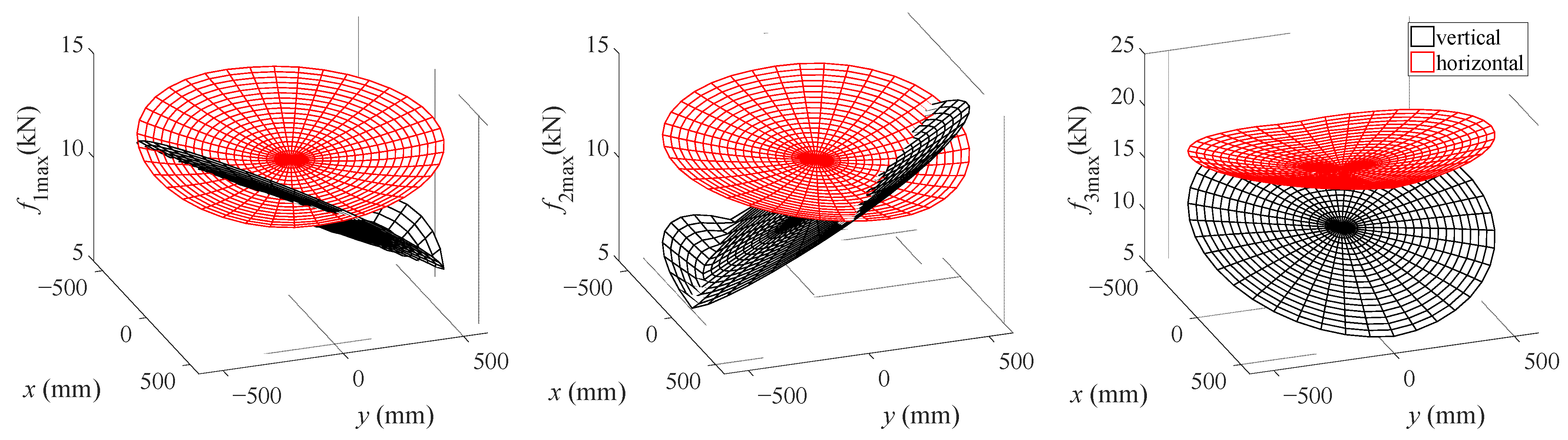
5.1. Influence of Hybrid Robot Placement Direction on Dynamic Performance

In practical application, the hybrid robot can be vertically or horizontally placed as shown in Figure 7. With different placement direction, gravity has a different effect on the dynamic performance. The inertial and geometric parameters of the robot are listed in the Appendix A. The indices f_gi (i = 1, 2, 3) and f_imax (i = 1, 2, 3) in the middle layer of the workspace are calculated by the MultiStart solver of Matlab 2016b, as shown in Figure 8 and Figure 9, and ${\overline{f}}_{i\max }$ is listed in Table 1. Figure 8 shows that when the robot is placed vertically, the motor of a limb needs to provide tension for the gravity term in the workspace near the limb, but to provide thrust in the workspace away from the limb. When the robot is placed horizontally, limbs 1 and 2 always need to provide a greater tension for the gravity term, and limb 3 always needs to provide a greater thrust for the gravity term.

Figure 7. Different placement directions of hybrid robot.

Figure 8. Distributions of gravity term of driving force in the middle layer of the workspace: (a) vertical; (b) horizontal.

Figure 9. Distributions of f_imax in the middle layer of the workspace in vertical and horizontal placement.

Table 1. Global performance indices in vertical and horizontal placement (unit: kN).

Global Index	Vertical	Horizontal
${\overline{f}}_{1\max }$	9.56	12.04
${\overline{f}}_{2\max }$	9.56	12.04
${\overline{f}}_{3\max }$	11.85	18.62

Figure 9 shows that in most workspaces, a smaller maximum absolute value of driving force is required in vertical placement than in horizontal placement. Only when the end-effector is close to a limb, the maximum absolute value of the driving force of the limb in vertical placement will be greater than that in horizontal placement. The results in Table 1 show that the average maximum absolute value of driving force in vertical placement is smaller, especially ${\overline{f}}_{3\max }$ is 36.36% less than that in horizontal placement, which indicates that the vertical placement is beneficial to the dynamics of the hybrid robot.

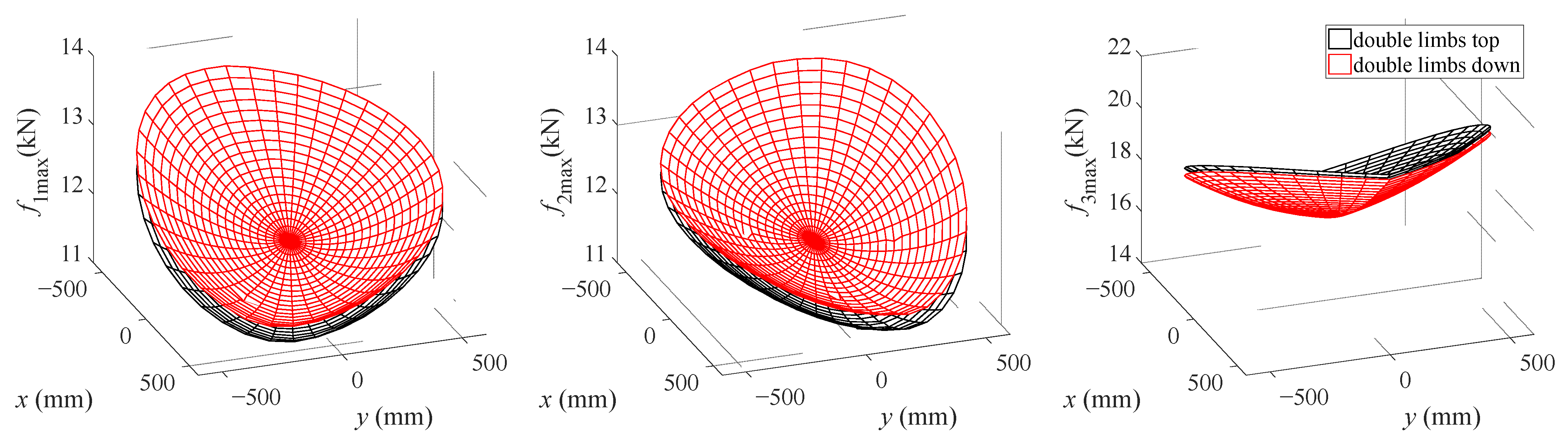
5.2. Effect of the Position of Double Symmetric Limbs on the Dynamic Performance

The arrangement of the limbs in horizontal placement will also affect the dynamic characteristics of the robot. The three limbs of the parallel mechanism in hybrid robot are usually arranged symmetrically due to the symmetrical structure of the mechanism, so there are two cases of double limbs on the top and double limbs on the bottom. The indices f_gi (i = 1, 2, 3) and f_imax (i = 1, 2, 3) in the middle layer of the workspace in the two cases are calculated by the MultiStart solver of Matlab 2016b, as shown in Figure 10 and Figure 11, and ${\overline{f}}_{i\max }$ is listed in Table 2. Figure 10 shows that when the double limbs are on the top, the double limbs need to provide tension for the gravity term of driving force while limb 3 needs to provide thrust for the gravity term of driving force; when the double limbs are on the bottom, the double limbs need to provide thrust for the gravity term of driving force while limb 3 needs to provide tension for the gravity term of driving force.

Figure 10. Distributions of gravity term of driving force in the middle layer of the workspace: (a) double limbs on the top; (b) double limbs on the bottom.

Figure 11. Distributions of f_imax in the middle layer of the workspace in different arrangements of the limbs.

Table 2. Global performance indices in different arrangements of the limbs (unit: kN).

Global index	Double Limbs on the Top	Double Limbs on the Bottom
${\overline{f}}_{1\max }$	12.04	12.26
${\overline{f}}_{2\max }$	12.04	12.26
${\overline{f}}_{3\max }$	18.62	18.36

Figure 11 and Table 2 show that when the double limbs are on the top, limbs 1 and 2 require smaller average maximum absolute values of driving force while limb 3 requires larger average maximum absolute values of the driving force, which indicates that the arrangement of the limbs has different effects on the dynamic performance of different limbs. Considering that the double limbs and the worktable or workpiece are prone to interference when the double limbs are on the bottom, the double limbs are often on the top when the robot is placed horizontally in practical application.

6. Conclusions

In this paper, the complete dynamic equation of a 5-DOF hybrid robot is formulated. A dynamic evaluation index taking velocity and gravity terms in the dynamic model into consideration is proposed. Then, the effect of the placement direction of the robot and the arrangement mode of the double symmetric limbs on the dynamics is investigated. The conclusions are drawn as follows:

(1)

The maximum absolute value of the driving force of the robot at given motion limits of the end-effector can be regarded as the dynamic evaluation index of the hybrid robot.

(2)

The influence of placement direction on the dynamics of the hybrid is investigated, and the results indicate that vertical placement is beneficial to the dynamics of the hybrid robot.

(3)

The effect of the position of the double limbs on the dynamic performance is investigated. The results show that when double limbs are arranged on top, the average dynamic performance of the double limbs can be improved, while the dynamic performance of the third limb will be slightly deteriorated.

References

- Orsino, R.M.M.; Coelho, T.A.H.; Pesce, C.P. Analytical mechanics approaches in the dynamic modelling of Delta mechanism. Robotica 2015, 33, 953–973. [Google Scholar] [CrossRef]
- Wu, J.; Wang, J.S.; You, Z. An overview of dynamic parameter identification of robots. Robot. Cim.-Int. Manuf. 2010, 26, 414–419. [Google Scholar] [CrossRef]
- Si, G.N.; Chen, F.H.; Zhang, X.P. Comparison of the dynamic performance of planar 3-DOF parallel manipulators. Machines 2022, 10, 233. [Google Scholar] [CrossRef]
- Chanal, H.; Guichard, A.; Blaysat, B.; Caro, S. Elasto-dynamic modeling of an over-constrained parallel kinematic machine using a beam model. Machines 2022, 10, 200. [Google Scholar] [CrossRef]
- Lee, G.; Park, S.; Lee, D.; Park, F.C.; Jeong, J.I.; Kim, J. Minimizing energy consumption of parallel mechanisms via redundant actuation. IEEE-ASME Trans. Mech. 2015, 20, 2805–2812. [Google Scholar] [CrossRef]
- Wu, J.; Gao, Y.; Zhang, B.B.; Wang, L. Workspace and dynamic performance evaluation of the parallel manipulators in a spray-painting equipment. Robot. Cim.-Int. Manuf. 2017, 44, 199–207. [Google Scholar] [CrossRef]
- Merlet, J.P. Determination of the orientation workspace of parallel manipulators. J. Intell. Robot. Syst. 1995, 13, 143–160. [Google Scholar] [CrossRef]
- Karger, A.; Husty, M. Classification of all self-motions of the original Stewart-Gough platform. Comput. Aided Des. 1998, 30, 205–215. [Google Scholar] [CrossRef]
- Luces, M.; Mills, J.K.; Benhabib, B. A review of redundant parallel kinematic mechanisms. J. Intell. Robot. Syst. 2017, 86, 175–198. [Google Scholar] [CrossRef]
- Xu, P.; Cheung, C.F.; Li, B.; Wang, C.; Zhao, C. Design, dynamic analysis, and experimental evaluation of a hybrid parallel-serial polishing machine with decoupled motions. J. Mech. Robot. 2021, 13, 061008. [Google Scholar] [CrossRef]
- Liu, S.; Sun, Y.; Peng, G.; Xue, Y.; Hnydiuk-Stefan, A.; Li, Z. Development of a novel 6-DOF hybrid serial-parallel mechanism for pose adjustment of large-volume components. Proc. Inst. Mech. Eng. Part C J. Mech. Eng. Sci. 2021, 236, 2099–2114. [Google Scholar] [CrossRef]
- Wang, Z.; Li, Y.; Sun, P.; Luo, Y.; Chen, B.; Zhu, W. A multi-objective approach for the trajectory planning of a 7-DOF serial-parallel hybrid humanoid arm. Mech. Mach. Theory 2021, 165, 104423. [Google Scholar] [CrossRef]
- Wu, J.; Yu, G.; Gao, Y.; Wang, L. Mechatronics modeling and vibration analysis of a 2-DOF parallel manipulator in a 5-DOF hybrid machine tool. Mech. Mach. Theory 2018, 121, 430–445. [Google Scholar] [CrossRef]
- Gao, Z.; Zhang, D. Performance analysis, mapping, and multiobjective optimization of a hybrid robotic machine tool. IEEE Trans. Ind. Electron. 2015, 62, 423–433. [Google Scholar] [CrossRef]
- Lai, Y.-L.; Liao, C.-C.; Chao, Z.-G. Inverse kinematics for a novel hybrid parallel–serial five-axis machine tool. Robot. Cim.-Int. Manuf. 2018, 50, 63–79. [Google Scholar] [CrossRef]
- Zhang, J.; Zhao, Y.; Dai, J. Compliance modeling and analysis of a 3-RPS parallel kinematic machine module. Chin. J. Mech. Eng. 2014, 27, 703–713. [Google Scholar] [CrossRef]
- Jin, Y.; Bi, Z.M.; Liu, H.T.; Higgins, C.; Price, M.; Chen, W.H.; Huang, T. Kinematic analysis and dimensional synthesis of Exechon parallel kinematic machine for large volume machining. J. Mech. Robot. 2015, 7, 041004. [Google Scholar] [CrossRef]
- Joshi, S.A.; Tsai, L.-W. The kinematics of a class of 3-DOF, 4-legged parallel manipulators. J. Mech. Design. 2003, 125, 52–60. [Google Scholar] [CrossRef]
- Joshi, S.; Tsai, L.-W. A comparison study of two 3-DOF parallel manipulators: One with three and the other with four supporting legs. IEEE Trans. Robot. Autom. 2003, 19, 200–209. [Google Scholar] [CrossRef]
- Liu, X.-J.; Han, G.; Xie, F.; Meng, Q. A novel acceleration capacity index based on motion/force transmissibility for high-speed parallel robots. Mech. Mach. Theory 2018, 126, 155–170. [Google Scholar] [CrossRef]
- Briot, S.; Caro, S.; Germain, C. Design procedure for a fast and accurate parallel manipulator. J. Mech. Robot. 2017, 9, 061012. [Google Scholar] [CrossRef]
- Merlet, J.P. Solving the forward kinematics of a Gough-type parallel manipulator with interval analysis. Int. J. Robot. Res. 2004, 23, 221–235. [Google Scholar] [CrossRef]
- Kumar, S.; Martensen, J.; Mueller, A.; Kirchner, F. Model simplification for dynamic control of series-parallel hybrid robots—A representative study on the effects of neglected dynamics. In Proceedings of the IEEE/RSJ International Conference on Intelligent Robots and Systems (IROS), Macau, China, 4–8 November 2019. [Google Scholar]
- Felis, M.L. RBDL: An efficient rigid-body dynamics library using recursive algorithms. Auton. Robot. 2017, 41, 495–511. [Google Scholar] [CrossRef]
- Li, M.; Huang, T.; Mei, J.; Zhao, X.; Chetwynd, D.G.; Hu, S.J. Dynamic formulation and performance comparison of the 3-DOF modules of two reconfigurable PKM—The Tricept and the TriVariant. J. Mech. Des. 2005, 127, 1129–1136. [Google Scholar] [CrossRef]
- Zhang, H.-Q.; Fang, H.-R.; Jiang, B.-S.; Wang, S.-G. Dynamic performance evaluation of a redundantly actuated and over-constrained parallel manipulator. Int. J. Autom. Comput. 2019, 16, 274–285. [Google Scholar] [CrossRef]
- Shao, H.; Zhang, H.; Yan, W. Dynamic modeling and performance optimization of a 2-PRU-PPRC 2T1R redundant parallel manipulator. In Proceedings of the 9th IEEE Annual International Conference on Cyber Technology in Automation, Control, and Intelligent Systems (IEEE-CYBER), Suzhou, China, 29 July–2 August 2019. [Google Scholar]
- Rao, C.; Xu, L.; Chen, Q.; Ye, W. Dynamic modeling and performance evaluation of a 2UPR-PRU parallel kinematic machine based on screw theory. J. Mech. Sci. Technol. 2021, 35, 2369–2381. [Google Scholar] [CrossRef]
- Han, J.; Shan, X.; Liu, H.; Xiao, J.; Huang, T. Fuzzy gain scheduling PID control of a hybrid robot based on dynamic characteristics. Mech. Mach. Theory 2023, 184, 105283. [Google Scholar] [CrossRef]
- Hao, Q. Optimization Design and Dynamic Control of a 2-DoF Planar Parallel Manipulator. Ph.D. Thesis, Tsinghua University, Beijing, China, 2011. [Google Scholar]
- Asada, H. A geometrical representation of manipulator dynamics and its application to arm design. J. Dyn. Syst.-T ASME 1983, 105, 131–142. [Google Scholar] [CrossRef]
- Yoshikawa, T. Dynamic manipulability of robot manipulators. J. Robot. Syst. 1985, 2, 113–124. [Google Scholar]
- Chen, M.; Zhang, Q.; Qin, X.; Sun, Y. Kinematic, dynamic, and performance analysis of a new 3-DOF over-constrained parallel mechanism without parasitic motion. Mech. Mach. Theory 2021, 162, 104365. [Google Scholar] [CrossRef]
- Kim, Y.; Desa, S. The definition, determination, and characterization of acceleration sets for spatial manipulators. Int. J. Robot. Res. 1993, 12, 572–587. [Google Scholar] [CrossRef]
- Bowling, A.; Kim, C.H. Dynamic performance analysis for non-redundant robotic manipulators in contact. In Proceedings of the 20th IEEE International Conference on Robotics and Automation (ICRA), Taipei, Taiwan, 14–19 September 2003. [Google Scholar]
- Xie, S.; Hu, K.; Liu, H.; Wan, Y. Dynamic modeling and performance analysis of a new redundant parallel rehabilitation robot. IEEE Access 2020, 8, 222211–222225. [Google Scholar] [CrossRef]
- Zhao, Y.J.; Gao, F. Dynamic formulation and performance evaluation of the redundant parallel manipulator. Robot. Cim.-Int. Manuf. 2009, 25, 770–781. [Google Scholar] [CrossRef]
- Ye, H.; Wang, D.; Wu, J.; Yue, Y.; Zhou, Y. Forward and inverse kinematics of a 5-DOF hybrid robot for composite material machining. Robot. Cim.-Int. Manuf. 2020, 65, 101961. [Google Scholar] [CrossRef]
- Zhang, D.; Xu, Y.; Yao, J.; Zhao, Y. Design of a novel 5-DOF hybrid serial-parallel manipulator and theoretical analysis of its parallel part. Robot. Cim.-Int. Manuf. 2018, 53, 228–239. [Google Scholar] [CrossRef]
- Wang, X.J.; Wu, J.; Wang, Y.T. Dynamics evaluation of 2UPU/SP parallel mechanism for a 5-DOF hybrid robot considering gravity. Robot. Auton. Syst. 2021, 135, 103675. [Google Scholar] [CrossRef]
Disclaimer/Publisher’s Note: The statements, opinions and data contained in all publications are solely those of the individual author(s) and contributor(s) and not of MDPI and/or the editor(s). MDPI and/or the editor(s) disclaim responsibility for any injury to people or property resulting from any ideas, methods, instructions or products referred to in the content. |
© 2023 by the authors. Licensee MDPI, Basel, Switzerland. This article is an open access article distributed under the terms and conditions of the Creative Commons Attribution (CC BY) license (https://creativecommons.org/licenses/by/4.0/).