Active Fault Diagnosis and Control of a Morphing Multirotor Subject to a Stuck Arm ^†

Abstract

In this paper, we propose a fault tolerant control law for a morphing quadrotor, where the considered morphing ability is that of extendable/telescopic arms. This quite recent class of systems is able to provide a good trade-off between payload capabilities, maneuverability, and space occupancy. However, such degrees of freedom require dedicated servomotors, which in turn implies more possible faults. Thus, the problem of diagnosis for the telescopic servo motors subject to a stuck fault is considered. System symmetries are exploited and used in a residual generator design, which triggers an active fault isolation/identification phase. External disturbances are also taken into account and estimated through a nonlinear disturbance observer. A classical double-loop controller closes the loop, providing an overall control system structure that follows the disturbance observer-based control paradigm. The control scheme is validated through realistic numerical simulations, and the closed-loop performances are analyzed.

1. Introduction

The size of Unmanned Aerial Vehicles (UAVs) is not a detail, as for different sizes different challenges arise. For example, mini, micro, and nano UAVs [1,2] have been largely studied in the past years, but the downside of miniaturization is the lower payload, which is not acceptable in many applications. On the contrary, maneuvering becomes more involved as the vehicle mass and inertia increase, and, therefore, a trade-off between the system bandwidth and the maximum payload is a current research problem. The solution is investigated through two main layers, the actuation and the mechanical system structure of the UAV. Concerning the first, variable pitch actuators are the most remarkable example [3]. Among the advantages, they show faster time response, leading to reduced power requirements and motor size [4]. It is worth noting that variable pitch configurations allow downward thrusts (without reversing the angular speed of the propellers), thus showing increased fault tolerant capabilities [5,6]. Regarding the second, two alternative ways have been investigated to reduce the size without compromising payload capabilities. The first class to note is the so-called folding multirotors, which can be split into multi-joint structures [7] and continuous deformable structures, such as origami foldable structures [8]. Such systems consist of UAVs being able to be folded/disassembled after the operation, even reaching a pocket-size dimension for a comfortable transportation [9]. During the operation, however, they exhibit a fixed structure, and no system reconfiguration is allowed, except for exceptional triggering events [10]. The second class is represented by reconfigurable or morphing multirotors that allow for in-flight morphing of the UAV [11]. The most common degrees of freedom are represented by extensible arms [12] (telescopic or sliding arms) and rotating arms [13,14]. By transforming its structure, the UAV does modify its space occupancy, its inertia [15], and its maneuverability based on the required task [16]. From a control law perspective, the morphing ability represents an additional degree of freedom [17], which is usually handled by a continuous refresh of the center of mass, the inertia and the allocation matrices, leading to a morphology-dependent control. Thus, assuming the transformation is relatively slow, only minor modifications need to be applied to the most common control techniques, such as proportional integral control [18], linear quadratic regulator [13], and active disturbance rejection control [19]. External disturbances cope with the system dynamics in the same way as standard multirotors. Many estimation methods have been proposed in the literature, ranging from specific oriented solutions (see [20] and references therein) to general purpose solutions such as Disturbance Observer-Based Control (DOBC), where the disturbance attenuation is provided by an observer-based feed-forward law [21]. Finally, the transformation ability implies additional actuation degrees, which in turn means possible additional faults with respect to those of standard multirotors, due to the servomotors involved in the morphing mechanisms. Such an acquired over-actuation brings the need for directional residues, which we can find in the observer-based residual generators [22], a possible solution with strong evidence in the literature and general purpose results.

In this paper, we propose an active fault-tolerant control scheme for morphing quadrotors, where the terminology fault-tolerant refers to a control law which is able to cope with faults, and by active it is meant that the fault is directly estimated and feedforwarded in the control loop [23,24]. The solution extends our previous work [25], where a DOBC scheme which copes with external disturbances was designed by joining a Nonlinear Disturbance Observer (NDO) with an inner/outer loop feedback linearization control law. Thus, the main objective is that of extending [25] by considering stuck faults in the morphology-related servomotors. The considered morphing ability is that of telescopic arms (extendable arms), which represent a promising solution to flight into narrow spaces while keeping payload and maneuvering capabilities [12]. The diagnosis is performed by exploiting the system symmetries. It turns out that a classical bank of observers (i.e., a residual generator) is not sufficient to cope with the problem, which represents a main step for the solution. In particular, after one residual component triggers, an active fault isolation, and identification phase is required, i.e., the isolation/identification is performed by the injection of a specific class of control inputs.

The paper is structured as follows. In Section 2, we propose and detail the mathematical model of a telescopic quadrotor. System symmetries are discussed and exploited in Section 3. Section 4 handles the overall fault diagnosis, both the residual generator and the active fault diagnosis. Section 5 briefly recalls the DOBC solution provided in [25], which closes the loop. Finally, numerical simulations are discussed in Section 6, where masses and dimensions are taken from commercial components, and practical real-world problems (e.g., input saturation, sensor noise, and different sample rate between the two control loops) are also taken into account.

2. Mathematical Model

Remark 1.

From now on, standard basis vectors of ${\mathbb{R}}^n$ are denoted as $e_k$ with $k=1,\dots ,n$, $diag(·)$ denoting the diagonal matrix with the elements of the argument in the main diagonal, and $col(·)$ denoting a column vector whose elements are listed in the argument.

Telescopic quadrotors are quadrotors with extendable (telescopic) arms. The whole system can be considered as a collection of $N=17$ rigid bodies subject to constraints. The frame is denoted with $B_0$, while the remaining bodies are denoted with $B_{i,j}$, where $i\in \{1,2,3,4\}$ denotes the arm and $j\in \{1,2,3,4\}$ denotes the component (Figure 1). For each arm, we denote with $l_i$ the length of the arm.

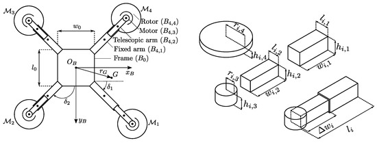
Figure 1. Schematic representations of the morphing quadrotor (left) and the telescopic arm (right). Each arm is independently controlled by a servomotor, possibly leading to an asymmetric structure. The telescopic arm is considered as a union of four bodies, where for each one the geometric dimensions are assumed known. For control purposes, as well as for a better interpretation, the overall arm length $l_i$ will be always made explicit. The bodies’ centers of mass are depicted with a bold point, and we assume they coincide with each body’s geometric center.

Two reference frames are considered. The first reference frame is an earth fixed frame $R_E=(O_E,{\mathcal{T}}_E)$ with a right-handed orthonormal triad ${\mathcal{T}}_E=(x_E,y_E,z_E)$, which is assumed to be inertial for simplicity. Then, a second frame $R_B=(O_B,{\mathcal{T}}_B)$ with a right-handed orthonormal triad ${\mathcal{T}}_B=(x_B,y_B,z_B)$ is placed in the geometric center $O_B$ of the frame $B_0$. Reference frame $R_B$ is a rest frame for the quadrotor frame, i.e., it is a body fixed frame for $B_0$ (see Figure 1). For slowly varying arm lengths, the telescopic quadrotor can be approximated as a rigid body that has its own center of mass, denoted as G, and described by the following equations [26]

$$\begin{array}{cc}\hfill m{\ddot{p}}_F& =-k_t{\dot{p}}_F-m{R}_B^E(\dot{\omega }\times r_G^B\left(l\right)+\omega \times (\omega \times r_G^B\left(l\right)))+F_g^E+R_B^E{F}_m^B\left(l\right)+F_w^E\hfill \\ \hfill J\left(l\right)\dot{\omega }& =-k_r\omega -\omega \times J\left(l\right)\omega +M_m^B\left(l\right)\hfill \\ \hfill \dot{\eta }& =T\left(\eta \right)\omega ,\hfill \end{array}$$

(1)

where each term is as follows:

• $p_F=\overrightarrow{O_E{O}_B}=\mathrm{col}(x_F,y_F,z_F)$ is the position of $R_B$ (decomposed in $R_E$);
• $\omega =\mathrm{col}(p,q,r)$ is the angular velocity of $R_B$ relative to $R_E$ (decomposed in $R_B$);
• m is the total system mass, g is the gravitational acceleration, and $k_t$ and $k_r$ are the linear and angular friction coefficients;
• $F_g^E=mg{e}_3$ and $F_w^E$ are the gravitational and the (unknown) wind forces (decomposed in $R_E$);
• $l=\mathrm{col}(l_1,\dots ,l_4)$ is the vector containing the arm lengths of each motor (see Figure 1);
• $r_G^B\left(l\right)=\overrightarrow{O_{B}G}$ is the arm-dependent center of mass (decomposed in $R_B$);
• $J\left(l\right)$ is the arm-dependent inertia matrix of the overall system, relative to the center of mass;
• $F_m^B\left(l\right)$ and $M_m^B\left(l\right)$ are the arm-dependent thrust and torque due to the actuators (both decomposed in $R_B$);
• $\eta =\mathrm{col}(\phi ,\theta ,\psi )$ is the vector composed by the roll ($\phi$), pitch ($\theta$), and yaw $\left(\psi \right)$ angles, which let us express the rotation matrix from $R_B$ to $R_E$, denoted as $R_B^E$, as

  $$R_B^E=R_B^E\left(\eta \right)=\left[\begin{array}{ccc}{c}_{\psi }{c}_{\theta }& c_{\psi }{s}_{\phi }{s}_{\theta }-c_{\phi }{s}_{\psi }& s_{\phi }{s}_{\psi }+c_{\phi }{c}_{\psi }{s}_{\theta }\\ c_{\theta }{s}_{\psi }& c_{\phi }{c}_{\psi }+s_{\phi }{s}_{\psi }{s}_{\theta }& c_{\phi }{s}_{\psi }{s}_{\theta }-c_{\psi }{s}_{\phi }\\ -s_{\theta }& c_{\theta }{s}_{\phi }& c_{\phi }{c}_{\theta }\end{array}\right],$$

  (2)

  where $cos(·)=c_{(·)}$ and $sin(·)=s_{(·)}$ are considered for the sake of brevity;
• $T\left(\eta \right)$ is the kinematic coordinate transformation related to the adopted roll–pitch–yaw rotation.

Remark 2.

In (1), the time dependencies are omitted for the sake of brevity. We remark that both l and η are time-dependent variables.

Remark 3.

In the following, the arm and angle dependencies are often omitted for the sake of brevity.

Remark 4.

The following common approximations were made in the model [6]:

• no torques due to the wind are considered;
• additional forces and torques due to blade flapping are of a smaller magnitude and neglected;
• the friction force is assumed to be linear, with proportional coefficients $k_t$, $k_r$.

For a brief description, let us denote the mass of the body $B_{i,j}$ with $m_{i,j}$, and the vector connecting the body frame with the body $B_{i,j}$ with $r_{i,j}^B=\overrightarrow{O_B{G}_{i,j}}$ (decomposed in $R_B$). The remaining variables are as follows.

2.1. Total Mass

The total mass m is the constant real number

$$m=m_0+\sum _{i=1}^4\sum _{j=1}^4{m}_{i,j}.$$

(3)

2.2. Center of Mass

The center of mass is the arm-dependent vector

$$r_G^B=\frac{1}{m}\left(m_0{r}_0^B+\sum _{i=1}^4\sum _{j=1}^4{m}_{i,j}{r}_{i,j}^B\right).$$

(4)

2.3. Inertia Matrix

The inertia is the arm-dependent matrix

$$J=J_0+\sum _{i=1}^4\sum _{j=1}^4{J}_{i,j},$$

(5)

where each $J_{i,j}$ denotes the inertia of the body $B_{i,j}$ relative to axes which are parallel to $x_B$, $y_B$, and $z_B$, and which pass through the center of mass, i.e., parallel the $R_B$ axes. In turn, each $J_{i,j}$ is dependent from the geometric dimensions, i.e., from the width $w_{i,j}$, the length $l_{i,j}$, the height $h_{i,j}$, and the orientation of $B_{i,j}$ (see Figure 1). Denoting the angle of the i-th arm with ${\delta }_i$ (around $z_B$, from $x_B$, as depicted in Figure 1), the orientation of the body $B_{i,j}$ is described by the rotation matrix

$$\begin{array}{cccc}\hfill R_{i,j}^B=R_{i,j}^B\left({\delta }_i\right)& =\left[\begin{array}{ccc}cos\left({\delta }_i\right)& -sin\left({\delta }_i\right)& 0\\ sin\left({\delta }_i\right)& cos\left({\delta }_i\right)& 0\\ 0& 0& 1\end{array}\right],\hfill & \hfill i& =1,2,3,4,j=1,2,3,4.\hfill \end{array}$$

(6)

Using the $R_{i,j}^B$s and $r_{i,j}^B$s, it is possible to express the inertia matrices $J_{i,j}$ through the parallel axis theorem. The reader can refer to [13,15,25] for details about the calculation of each $J_{i,j}$.

2.4. Actuation Force and Moment

For each propeller i, let $f_i$ be the (scalar) upward lift force. Then $f_i^B=-f_i{e}_3$ is the vector lift force (decomposed in $R_B$), and the actuation force is

$$F_m^B=\sum _{i=1}^4{f}_i^B=-\sum _{i=1}^4{f}_i{e}_3.$$

(7)

The actuation torque $M_m^B$ can be decomposed into the thrust component and the drag component, namely $M_m^B=M_{thrust}^B+M_{drag}^B$. In particular, we have

$$\begin{array}{cc}\hfill M_{thrust}^B& =-\sum _{i=1}^4\left((r_{i,4}^B-r_G^B)\times f_i{e}_3\right),\hfill \end{array}$$

(8)

$$\begin{array}{cc}\hfill M_{drag}^B& =\sum _{i=1}^4{c}_{w_i}\frac{c_D}{c_L}{f}_i{e}_3,\hfill \end{array}$$

(9)

where $c_L$ and $c_D$ are the lift and drag coefficients, while $c_{w_i}=+1$ if the i-th motor rotates counter-clockwise, and $c_{w_i}=-1$ otherwise.

2.5. Inputs and Faults

Each lift force $f_i$ is assumed directly controlled, hence the vector $u=\mathrm{col}(f_1,f_2,f_3,f_4)$ serves as control input. The extension of each arm $l_i$ is performed by a servomotor, which can be affected by a stuck fault. If $l_{ni}$ denotes the nominal length (the reference for $l_i$), the servomotor provides

$$l_i=\left\{\begin{array}{cc}{l}_{n_i}\hfill & \mathrm{if}\mathrm{the}i\text{-}\mathrm{th}\mathrm{servomotor}\mathrm{is}\mathrm{healthy}\hfill \\ {\overline{l}}_i\hfill & \mathrm{if}\mathrm{the}i\text{-}\mathrm{th}\mathrm{servomotor}\mathrm{is}\mathrm{stuck},\hfill \end{array}\right.$$

(10)

where in case of a stuck fault, the constant ${\overline{l}}_i$ is unknown. Introducing the stuck offset $s_o=\mathrm{col}(s_{01},s_{02},s_{03},s_{04})$, where $s_{oi}={\overline{l}}_i-l_{ni}$ is the stuck offset of the i-th arm, we have

$$l=l_n+s_o.$$

(11)

Remark 5.

In the following, the assumption of at most one stuck fault at a time is made, that is, if $s_{oi}\ne 0$ for some i, then $s_{oj}=0$ for $j\ne i$. In these terms, Fault Detection (FD) consists of determining if $s_{oi}\ne 0$ for some i, Fault Isolation (FI) consists of determining which i is such that $s_{oi}\ne 0$, and Fault Identification (FId) consists of the estimation of ${\overline{l}}_i$.

Remark 6.

Both u and $l_n$ are available inputs. The inputs u are fast and can be used for actual flight control; on the other hand, the inputs $l_n$ are slow, and commonly set by an external module for specific maneuvers (e.g., a supervisory module which commands a shrinking/enlarging phase). As such, only u will be used for the tracking control goal, while $l_n$ will play a main role in the active stuck fault isolation. To this end, let $l^{★}=\mathrm{col}(l_1^{★},l_2^{★},l_3^{★},l_4^{★})$ be the desired/optimal arm lengths provided by the external module; ideally, we would like to achieve $l=l^{★}$ by setting $l_n=l^{★}$. This will be not true during FI.

Remark 7.

In a matrix-like fashion, it is possible to rewrite $F_m^B$ and $M_m^B$ in terms of u as

$$\begin{array}{ccccc}\hfill F_m^B& =F_{1}u,\hfill & & \hfill M_m^B& =F_{2}u,\hfill \end{array}$$

(12)

where $F_1\in {\mathbb{R}}^{3\times 4}$ is the control force input matrix and $F_2$ is the so called control moment input matrix [27]. Trivially,

$$F_1=\left[\begin{array}{cccc}0& 0& 0& 0\\ 0& 0& 0& 0\\ -1& -1& -1& -1\end{array}\right],$$

(13)

while $F_2$ will be exploited later.

Remark 8.

Note that $r_G^B$, J and $F_2$ are arm-dependent and, as such, time-varying. These quantities can be calculated online. As such, in the next sections, their dependence on the arms’ length will be omitted for brevity.

3. Symmetries and Sensitivity

To design the fault detection, isolation, and identification policy of Section 4, the following symmetries are presented and will be exploited later.

• The arms are counter-clockwise numbered and equally distributed on the so-called “x” configuration, leading to the angles

  $$\begin{array}{cccc}\hfill {\delta }_i& =\frac{\pi }{4}+(i-1)\frac{\pi }{2}, \hfill & \hfill i& =1,\dots ,4.\hfill \end{array}$$

  (14)
• The overall geometry of each arm is identical to the others. In particular, the geometry constraints of each fixed arm $B_{i,1}$ and telescopic arm $B_{i,2}$ lead to

  $$w_{i,j}=w_{1,j},i=2,3,4,j=1,2,$$

  (15)

  $$l_{i,j}=l_{1,j},i=2,3,4,j=1,2,$$

  (16)

  $$h_{i,j}=h_{1,j},i=2,3,4,j=1,2,$$

  (17)

  while the geometry constraints of each motor $B_{i,3}$ and rotor $B_{i,4}$ lead to

  $$r_{i,j}=r_{1,j},i=2,3,4,j=3,4,$$

  (18)

  $$h_{i,j}=h_{1,j},i=2,3,4,j=3,4.$$

  (19)
• For each arm, the mass of each component is equal to the corresponding component of the other arms, which leads to

  $$m_{i,j}=m_{1,j},i=2,3,4,j=1,2,3,4.$$

  (20)
• Motors 1 and 3 are counter-clockwise, while 2 and 4 are clockwise, hence

  $$\begin{array}{cccc}\hfill c_{w_i}& ={(-1)}^{i+1}, \hfill & \hfill i& =1,2,3,4.\hfill \end{array}$$

  (21)
  Several implications follow.
• The total mass of the system is

  $$m=m_0+4(m_{1,1}+m_{1,2}+m_{1,3}+m_{1,4}).$$

  (22)
• Since ${\delta }_3={\delta }_1+\pi$ and ${\delta }_4={\delta }_2+\pi$, for each vector $v\in \mathrm{span}\{e_1,e_2\}$ we have

  $$\begin{array}{ccccc}\hfill R_{3,j}^{B}v& =-R_{1,j}^{B}v,\hfill & & \hfill j& =1,2,3,4,\hfill \end{array}$$

  (23)

  $$\begin{array}{ccccc}\hfill R_{4,j}^{B}v& =-R_{2,j}^{B}v,\hfill & & \hfill j& =1,2,3,4.\hfill \end{array}$$

  (24)

Remark 9.

The center of mass $r_G^B$ is linear in l. In particular, we have $r_G^B=K_{G}l$, where

$$K_G=\frac{\sqrt{2}}{2}\frac{m_{1,2}+m_{1,3}+m_{1,4}}{m}\left[\begin{array}{cccc}1& -1& -1& 1\\ 1& 1& -1& -1\\ 0& 0& 0& 0\end{array}\right].$$

(25)

See Appendix A.1 for details.

Remark 10.

The actuation torque $M_m^B$ is affine in l, that is, it can be rewritten as $M_m^B=v\left(u\right)+K_m\left(u\right)l$, where $v\left(u\right)\in {\mathbb{R}}^3$ and $K_m\left(u\right)\in {\mathbb{R}}^{3\times 4}$. Moreover, $v\left(u\right)$ is linear in u and it can be rewritten as $v\left(u\right)=K_{v}u$, where

$$K_v=\left[\begin{array}{cccc}-\frac{l_0}{2}& -\frac{l_0}{2}& \frac{l_0}{2}& \frac{l_0}{2}\\ \frac{w_0}{2}& -\frac{w_0}{2}& -\frac{w_0}{2}& \frac{w_0}{2}\\ \frac{c_D}{c_L}& -\frac{c_D}{c_L}& \frac{c_D}{c_L}& -\frac{c_D}{c_L}\end{array}\right].$$

(26)

Finally, the i-th column of $K_m\left(u\right)$, denoted as $K_m^i\left(u\right)$, is linear in u, that is $K_m^i\left(u\right)=D_{i}u$, where

$$D_i=R_{i,1}^B{E}_{2,i}-\frac{m_{1,2}+m_{1,3}+m_{1,4}}{m}{R}_{i,1}^B(E_{2,1}+E_{2,2}+E_{2,3}+E_{2,4}),$$

(27)

where $E_{i,j}\in {\mathbb{R}}^{3\times 4}$ is defined as a matrix with zero elements but the $i,j$ element which is equal to “1”. See Appendix A.2 for details.

Remark 11.

Defining $\overline{m}=\frac{m_{1,2}+m_{1,3}+m_{1,4}}{m}$, it is possible to rewrite $D_1,D_2,D_3,D_4$ in a matrix fashion as

$$\begin{array}{cccc}\hfill D_1& =R_{1,1}^B\left[\begin{array}{cccc}0& 0& 0& 0\\ 1-\overline{m}& -\overline{m}& -\overline{m}& -\overline{m}\\ 0& 0& 0& 0\end{array}\right],\hfill & \hfill D_2& =R_{2,1}^B\left[\begin{array}{cccc}0& 0& 0& 0\\ -\overline{m}& 1-\overline{m}& -\overline{m}& -\overline{m}\\ 0& 0& 0& 0\end{array}\right],\hfill \end{array}$$

(28)

$$\begin{array}{cccc}\hfill D_3& =R_{3,1}^B\left[\begin{array}{cccc}0& 0& 0& 0\\ -\overline{m}& -\overline{m}& 1-\overline{m}& -\overline{m}\\ 0& 0& 0& 0\end{array}\right],\hfill & \hfill D_4& =R_{4,1}^B\left[\begin{array}{cccc}0& 0& 0& 0\\ -\overline{m}& -\overline{m}& -\overline{m}& 1-\overline{m}\\ 0& 0& 0& 0\end{array}\right].\hfill \end{array}$$

(29)

Remark 12.

The control moment input matrix $F_2$ can be rewritten as

$$F_2=K_v+l_1{D}_1+\dots +l_4{D}_4.$$

(30)

Indeed, we have $M_m^B=F_{2}u$, and, at the same time,

$$\begin{array}{cc}\hfill M_m^B& =K_{v}u+K_m\left(u\right)l\hfill \end{array}$$

(31)

$$\begin{array}{cc}\hfill & =K_{v}u+\sum _{i=1}^4\left(l_i{D}_{i}u\right)\hfill \end{array}$$

(32)

$$\begin{array}{cc}\hfill & =(K_v+\sum _{i=1}^4\left(l_i{D}_i\right))u.\hfill \end{array}$$

(33)

Remark 13.

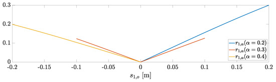
Consider the index

$$\frac{\left|\right|J\left(l_n\right)-J\left(l\right)\left|\right|}{\left|\right|J\left(l\right)\left|\right|},$$

(34)

where the demanded arm lengths $l_n$ differ from the actual ones for one component only. Each arm is demanded a length of α i.e., $l_n=col(\alpha ,\alpha ,\alpha ,\alpha )\triangleq \overline{\alpha }$, and the i-th arm is considered to have a stuck displacement $s_{o_i}$. Therefore, we consider the indexes

$$\begin{array}{cccc}\hfill r_{i,\alpha }\left(s_{oi}\right)& =\frac{\left|\right|J\left(\overline{\alpha }\right)-J(\overline{\alpha }+e_i{s}_{oi})\left|\right|}{\left|\right|J(\overline{\alpha }+e_i{s}_{oi})\left|\right|},\hfill & \hfill i& =1,\dots ,4.\hfill \end{array}$$

(35)

Figure 2 shows the numerical evaluation of the index $r_{1,\alpha }$. The indexes $r_{2,\alpha },r_{3,\alpha },r_{4,\alpha }$ are identical due to the symmetry of the system.

Figure 2. Sensitivity indexes for $J\left(l\right)$. The calculation is performed with the numerical parameters reported in Section 6.

For each index, the evaluation is performed for $\alpha =0.2$ (m), $\alpha =0.3$ (m), and $\alpha =0.4$ (m), which represent the (minimum, average, and maximum) lengths of the arms of the vehicle used in the numerical simulations, as described in Table 1. In the worst case, that is, when the stuck offset is $0.2$ (m), the variation of $\left|\right|J\left(l\right)\left|\right|$ is up to $30\%$. It is, however, reasonable to fix the arm set point in the middle range ($\alpha =0.3$ (m)), leading to a variation up to $15\%$. Thus, for the rest of the paper, the design is performed assuming $J\left(l\right)\approx J\left(l_n\right)$, which will be, therefore, simply written as J.

Table 1. Fault signature matrix of the fault classes ${\mathcal{C}}_1,{\mathcal{C}}_2$ provided by ${\Sigma }_{FDI}$. The isolation is achieved through the evaluation of the non-zero value of $r_1\left(t\right),r_2\left(t\right)$.

	${\mathcal{C}}_0$	${\mathcal{C}}_1$	${\mathcal{C}}_2$
$r_1\left(t\right)$	0	$\ne 0$	0
$r_2\left(t\right)$	0	0	$\ne 0$

4. Fault Detection, Isolation, and Identification

4.1. Fault Detection

Following [22], we approach the problem in the following way.

Definition 1.

A (fault detection) residual generator is a dynamic system with the structure

$$\begin{array}{cc}\hfill \dot{z}& =f(z,u,p_F,{\dot{p}}_F,\omega ,\eta ),\hfill \\ \hfill r& =h(z,u,p_F,{\dot{p}}_F,\omega ,\eta ),\hfill \end{array}$$

(36)

where $z\left(t\right)\in {\mathbb{R}}^{n_z}$ and $r\left(t\right)\in {\mathbb{R}}^{n_r}$, such that

1. 

whenever no fault occurs, $r\left(t\right)$ exhibits convergent dynamics;

2. 

whenever a fault occurs, at least one component of $r\left(t\right)$ does not exhibit convergent dynamics.

If (36) is a (fault detection) residual generator, then $r\left(t\right)$ is an (observer based) fault detection residue.

Remark 14.

In the common definitions, the fault detection residue $r\left(t\right)$ is a scalar one, that is, $r\left(t\right)\in \mathbb{R}$ for each t. This condition can be matched by considering the new residue $\left|\right|r\left(t\right)\left|\right|$.

Consider the dynamical system

$${\Sigma }_{FD}:\begin{array}{cc}\hfill \dot{z}& =-k_r{J}^{-1}\omega -J^{-1}(\omega \times J\omega )+J^{-1}v\left(u\right)+J^{-1}{K}_m\left(u\right)l_n+H(\omega -z)\hfill \\ \hfill r& =\omega -z,\hfill \end{array}$$

(37)

where $-H\in {\mathbb{R}}^{3\times 3}$ is a Hurwitz matrix.

Proposition 1.

If $u\left(t\right)\notin ker\left(D_i\right)$ for $i=1,\dots ,4$, then ${\Sigma }_{FD}$ is a (fault detection) residual generator.

Proof. 

The residue dynamics are

$$\dot{r}=-Hr+J^{-1}{K}_m{s}_o.$$

(38)

If no telescopic arm is stuck, then $s_o=0$, the residue r exhibits asymptotically stable dynamics. Let the j-th arm be the stuck one, i.e., let $s_{oj}\left(t\right)\ne 0$ and $s_{oi}\left(t\right)=0$ for $i\ne j$. The residue dynamics are then

$$\begin{array}{cc}\hfill \dot{r}& =-Hr+\left(J^{-1}{K}_m{e}_j\right)s_{oj}\hfill \end{array}$$

(39)

$$\begin{array}{cc}\hfill & =-Hr+\left(J^{-1}{D}_{j}u\right)s_{oj},\hfill \end{array}$$

(40)

and because $\left(J^{-1}{D}_{j}u\right)s_{oj}\ne 0$, $r\left(t\right)$ does not converge to the origin. □

4.2. Fault Isolation

Following again a simplified version of [22], we approach the fault isolation problem as follows. Let ${\mathcal{C}}_1,\dots ,{\mathcal{C}}_k$ be fault classes to isolate, and let us denote with ${\mathcal{C}}_0$ the absence of faults. We assume in every instant of time one ${\mathcal{C}}_i$ is active for some unknown i, while ${\mathcal{C}}_j$ is not active for every $j\ne i$.

Definition 2.

A (fault isolation) residual generator for ${\mathcal{C}}_1,\dots ,{\mathcal{C}}_k$ is a dynamical system with the structure

$$\begin{array}{cc}\hfill \dot{z}& =f(z,u,p_F,{\dot{p}}_F,\omega ,\eta ),\hfill \\ \hfill r_i& =h_i(z,u,p_F,{\dot{p}}_F,\omega ,\eta ),i=1,\dots ,k,\hfill \end{array}$$

(41)

where $z\left(t\right)\in {\mathbb{R}}^{n_z}$ and $r_i\left(t\right)\in \mathbb{R}$, such that

1. 

whenever ${\mathcal{C}}_0$ occurs, $r_i\left(t\right)$ exhibits convergent dynamics for $i=1,\dots ,k$;

2. 

whenever ${\mathcal{C}}_i$ occurs, for $i\in \{1,\dots ,k\}$, $r_i\left(t\right)$ does not exhibit convergent dynamics, while $r_j\left(t\right)$ exhibits convergent dynamics for each $j\ne i$.

If (41) is a (fault isolation) residual generator for ${\mathcal{C}}_1,\dots ,{\mathcal{C}}_k$, then $r\left(t\right)=\mathrm{col}(r_1\left(t\right),\dots ,r_k\left(t\right))$ is a (directional observer-based) fault isolation residue.

In our purpose, we define the fault classes

$$\begin{array}{cc}\hfill {\mathcal{C}}_0:& \mathrm{if}{s}_{o1}=s_{o2}=s_{o3}=s_{o4}=0,\hfill \end{array}$$

(42)

$$\begin{array}{cc}\hfill {\mathcal{C}}_1:& \mathrm{if}{s}_{o1}\ne 0\mathrm{or}{s}_{o3}\ne 0,\hfill \end{array}$$

(43)

$$\begin{array}{cc}\hfill {\mathcal{C}}_2:& \mathrm{if}{s}_{o2}\ne 0\mathrm{or}{s}_{o4}\ne 0.\hfill \end{array}$$

(44)

Consider the dynamical system

$${\Sigma }_{FDI}:\begin{array}{cc}\hfill {\dot{z}}_1& =-k_r{v}_1^T\omega -v_1^T(\omega \times J\omega )+v_1^{T}v\left(u\right)+v_1^T{K}_m\left(u\right)l_n+H_1(v_1^{T}J\omega -z_1)\hfill \\ \hfill {\dot{z}}_2& =-k_r{v}_2^T\omega -v_2^T(\omega \times J\omega )+v_2^{T}v\left(u\right)+v_2^T{K}_m\left(u\right)l_n+H_2(v_2^{T}J\omega -z_2)\hfill \\ \hfill r_1& =v_1^{T}J\omega -z_1\hfill \\ \hfill r_2& =v_2^{T}J\omega -z_2,\hfill \end{array}$$

(45)

where $H_1,H_2>0$, $v_1=-e_1+e_2$ and $v_2=e_1+e_2$.

Proposition 2.

If $u\notin ker\left(v_1^T{D}_i\right)$ for $i=1,3$ and $u\notin ker\left(v_2^T{D}_j\right)$ for $j=2,4$, then ${\Sigma }_{FDI}$ is a (fault isolation) residual generator for ${\mathcal{C}}_1,{\mathcal{C}}_2$.

Proof. 

We have

$$\begin{array}{cc}\hfill ker\left(D_1^T\right)& =ker\left(D_3^T\right)=\mathrm{span}\left\{e_1+e_2,e_3\right\},\hfill \end{array}$$

(46)

$$\begin{array}{cc}\hfill ker\left(D_2^T\right)& =ker\left(D_4^T\right)=\mathrm{span}\left\{e_1-e_2,e_3\right\},\hfill \end{array}$$

(47)

therefore, $v_1^T{D}_2=v_1^T{D}_4=v_2^T{D}_1=v_2^T{D}_3=0$ and

$$\begin{array}{ccccccccccc}\hfill v_1^T{D}_1& \ne 0\hfill & & \hfill v_1^T{D}_3& \ne 0\hfill & & \hfill v_2^T{D}_2& \ne 0\hfill & & \hfill v_2^T{D}_4& \ne 0.\hfill \end{array}$$

(48)

By differentiation, we have

$$\begin{array}{cc}\hfill {\dot{r}}_1& =-H_1{r}_1+\left(v_1^T{D}_{1}u\right)s_{o1}+\left(v_1^T{D}_{3}u\right)s_{o3}\hfill \end{array}$$

(49)

$$\begin{array}{cc}\hfill {\dot{r}}_2& =-H_2{r}_2+\left(v_2^T{D}_{2}u\right)s_{o2}+\left(v_1^T{D}_{4}u\right)s_{o4}.\hfill \end{array}$$

(50)

In the absence of faults, we have $s_{oi}\left(t\right)=0$ for $i=1,\dots ,4$, and, therefore, both $r_1\left(t\right)$ and $r_2\left(t\right)$ exhibit asymptotically stable (mutually decoupled) dynamics. In case of a fault of class ${\mathcal{C}}_1$, we have $s_{oi}\left(t\right)\ne 0$ for $i\in \{1,3\}$, and the residue dynamics are

$$\begin{array}{cc}\hfill {\dot{r}}_1& =-H_1{r}_1+\left(v_1^T{D}_{i}u\right)s_{oi}\hfill \end{array}$$

(51)

$$\begin{array}{cc}\hfill {\dot{r}}_2& =-H_2{r}_2,\hfill \end{array}$$

(52)

hence $r_2\left(t\right)$ exhibits an asymptotically stable dynamics, while $r_1\left(t\right)$ does not. Finally, in the case of a fault of class ${\mathcal{C}}_2$, we have $s_{oj}\left(t\right)\ne 0$ for $j\in \{2,4\}$, and the residue dynamics are

$$\begin{array}{cc}\hfill {\dot{r}}_1& =-H_1{r}_1\hfill \end{array}$$

(53)

$$\begin{array}{cc}\hfill {\dot{r}}_2& =-H_2{r}_2+\left(v_2^T{D}_{j}u\right)s_{oj},\hfill \end{array}$$

(54)

hence $r_1\left(t\right)$ exhibits an asymptotically stable dynamics, while $r_2\left(t\right)$ does not. □

Remark 15.

The fault signature matrix provided by Proposition (2) is summarized in Table 1. In practice, the isolation is provided through a threshold-based policy.

Remark 16.

Without a specific control input, the filter ${\Sigma }_{FDI}$ is not able to isolate which arm is stuck, but just to isolate the pairs $(1,3)$ and $(2,4)$. This is a consequence of the symmetries of the system, and the motivation for achieving active isolation in the following. The diagnostic information provided by $r_1\left(t\right)$ and $r_2\left(t\right)$ can, however, lead to finer isolation.

Let us split ${\mathcal{C}}_1$ and ${\mathcal{C}}_2$ into two subclasses each, considering that the overall fault classes

$$\begin{array}{cc}\hfill {\mathcal{C}}_0:& \mathrm{if}{s}_{o1}=s_{o2}=s_{o3}=s_{o4}=0,\hfill \end{array}$$

(55)

$$\begin{array}{cc}\hfill {\mathcal{C}}_1^{+}:& \mathrm{if}{s}_{o1}>0\mathrm{or}{s}_{o3}<0,\hfill \end{array}$$

(56)

$$\begin{array}{cc}\hfill {\mathcal{C}}_1^{-}:& \mathrm{if}{s}_{o1}<0\mathrm{or}{s}_{o3}>0,\hfill \end{array}$$

(57)

$$\begin{array}{cc}\hfill {\mathcal{C}}_2^{+}:& \mathrm{if}{s}_{o2}<0\mathrm{or}{s}_{o4}>0,\hfill \end{array}$$

(58)

$$\begin{array}{cc}\hfill {\mathcal{C}}_2^{-}:& \mathrm{if}{s}_{o2}>0\mathrm{or}{s}_{o4}<0.\hfill \end{array}$$

(59)

The residue generator ${\Sigma }_{FDI}$ can be modified for the isolation of the fault classes ${\mathcal{C}}_1^{+},{\mathcal{C}}_1^{-},{\mathcal{C}}_2^{+},{\mathcal{C}}_2^{-}$. To this end, consider the function $ramp:\mathbb{R}\to \mathbb{R}$ defined as

$$ramp\left(x\right)=\left\{\begin{array}{cc}x\hfill & x\ge 0\hfill \\ 0\hfill & x<0.\hfill \end{array}\right.$$

(60)

Note that the function $ramp\left(x\right)$ provides the absolute value of the arguments x whenever x is positive, while the function $ramp(-x)$ provides the absolute value for $x<0$. From now on, we will consider the following assumption.

Assumption 1.

The inequalities

$$\begin{array}{cccc}\hfill f_i\left(t\right)-\overline{m}(f_1\left(t\right)+f_2\left(t\right)+f_3\left(t\right)+f_4\left(t\right))& \ge {\gamma }_i,\hfill & \hfill i& =1,2,3,4,\hfill \end{array}$$

(61)

are satisfied for each t and for some ${\gamma }_1,{\gamma }_2,{\gamma }_3,{\gamma }_4>0$.

Remark 17.

In practice, we have $f_i\left(t\right)\ge 0$ for each i. Then, noting that $f_1\left(t\right)+f_2\left(t\right)+f_3\left(t\right)+f_4\left(t\right)$ is the upward lift force at time t, Assumption (61) bounds the displacement between the $f_i\left(t\right)$s. Thus, it bounds the motor torques, which is coherent with the saturation, as well as with the fact that during the flight the quadrotor exhibits relatively small angles. Additionally, because $f_i\left(t\right)\ne 0$ for each i, strictly positive control inputs are implied.

Lemma 1.

Consider ${\Sigma }_{FDI}$ as in Proposition (2) and let $\mathcal{C}$ be the actual fault class.

1. 

If $\mathcal{C}={\mathcal{C}}_0$, then $r_1\left(t\right)$ and $r_2\left(t\right)$ exhibits asymptotically stable dynamics.

2. 

If $\mathcal{C}={\mathcal{C}}_1^{+}$, then $r_2\left(t\right)$ exhibits asymptotically stable dynamics, while $r_1\left(t\right)>0$ is achieved in finite time.

3. 

If $\mathcal{C}={\mathcal{C}}_1^{-}$, then $r_2\left(t\right)$ exhibits asymptotically stable dynamics, while $r_1\left(t\right)<0$ is achieved in finite time.

4. 

If $\mathcal{C}={\mathcal{C}}_2^{+}$, then $r_1\left(t\right)$ exhibits asymptotically stable dynamics, while $r_2\left(t\right)>0$ is achieved in finite time.

5. 

If $\mathcal{C}={\mathcal{C}}_2^{-}$, then $r_1\left(t\right)$ exhibits asymptotically stable dynamics, while $r_2\left(t\right)<0$ is achieved in finite time.

Proof. 

Point 1 has been proven in Proposition (2), so let us discuss point 2. Direct calculations lead to

$$\begin{array}{cc}\hfill v_1^T{D}_{1}u\left(t\right)& =\sqrt{2}(f_1\left(t\right)-\overline{m}(f_1\left(t\right)+f_2\left(t\right)+f_3\left(t\right)+f_4\left(t\right)))\ge \sqrt{2}{\gamma }_1,\hfill \end{array}$$

(62)

$$\begin{array}{cc}\hfill v_1^T{D}_{3}u\left(t\right)& =-\sqrt{2}(f_3\left(t\right)-\overline{m}(f_1\left(t\right)+f_2\left(t\right)+f_3\left(t\right)+f_4\left(t\right)))\le -\sqrt{2}{\gamma }_3,\hfill \end{array}$$

(63)

$$\begin{array}{cc}\hfill v_2^T{D}_{2}u\left(t\right)& =-\sqrt{2}(f_2\left(t\right)-\overline{m}(f_1\left(t\right)+f_2\left(t\right)+f_3\left(t\right)+f_4\left(t\right)))\le -\sqrt{2}{\gamma }_2,\hfill \end{array}$$

(64)

$$\begin{array}{cc}\hfill v_2^T{D}_{4}u\left(t\right)& =\sqrt{2}(f_4\left(t\right)-\overline{m}(f_1\left(t\right)+f_2\left(t\right)+f_3\left(t\right)+f_4\left(t\right)))\ge \sqrt{2}{\gamma }_4.\hfill \end{array}$$

(65)

Since ${\mathcal{C}}_1^{+}$ is a sub-case of ${\mathcal{C}}_1$, we have already proved that $r_2\left(t\right)$ converges to zero. Let $s_{o1}\left(t\right)$ be strictly positive, that is, let $s_{o1}\left(t\right)\ge s_{min}>0$. The rate of $r_1\left(t\right)$ is

$${\dot{r}}_1=-H_1{r}_1+\left(v_1^T{D}_{1}u\right)s_{o1}\ge -H_1{r}_1+\sqrt{2}{\gamma }_1{s}_{min},$$

(66)

implying

$$r_1\left(t\right)\ge \left(r_1\left(0\right)-\frac{\sqrt{2}{\gamma }_1{s}_{min}}{H_1}\right)e^{-H_{1}t}+\frac{\sqrt{2}{\gamma }_1{s}_{min}}{H_1},$$

(67)

which becomes strictly positive in finite time, depending on $r_1\left(0\right)$ and $H_1$. Let us now explore the remaining possibility for ${\mathcal{C}}_1^{+}$, that is, $s_{o3}\left(t\right)\le -s_{max}$, for some $s_{max}>0$. The rate of $r_1\left(t\right)$ is

$${\dot{r}}_1=-H_1{r}_1+\left(v_1^T{D}_{3}u\right)s_{o3}\le -H_1{r}_1+\sqrt{2}{\gamma }_3{s}_{max},$$

(68)

implying

$$r_1\left(t\right)\ge \left(r_1\left(0\right)-\frac{\sqrt{2}{\gamma }_3{s}_{max}}{H_1}\right)e^{-H_{1}t}+\frac{\sqrt{2}{\gamma }_3{s}_{max}}{H_1},$$

(69)

which becomes strictly positive in finite time, depending on $r_1\left(0\right)$ and $H_1$. The remaining points proceed identically. □

Proposition 3.

Consider $u\left(t\right)\notin ker\left(v_1^T{D}_i\right)$ for $i=1,3$ and $u\left(t\right)\notin ker\left(v_2^T{D}_j\right)$ for $j=2,4$. Then, the system ${\Sigma }_{FDI}$ together with the new output functions

$$\begin{array}{cc}\hfill r_1^{+}& =ramp(v_1^{T}J\omega -z_1)\hfill \end{array}$$

(70)

$$\begin{array}{cc}\hfill r_1^{-}& =ramp(-v_1^{T}J\omega +z_1)\hfill \end{array}$$

(71)

$$\begin{array}{cc}\hfill r_2^{+}& =ramp(v_2^{T}J\omega -z_2)\hfill \end{array}$$

(72)

$$\begin{array}{cc}\hfill r_2^{-}& =ramp(-v_2^{T}J\omega +z_2)\hfill \end{array}$$

(73)

is a (fault isolation) residual generator for ${\mathcal{C}}_1^{+},{\mathcal{C}}_1^{-},{\mathcal{C}}_2^{+},{\mathcal{C}}_2^{-}$.

Proof. 

Just merge Lemma (1) with the fact that

$$\begin{array}{cccc}\hfill r_1^{+}\left(t\right)& =ramp\left(r_1\left(t\right)\right),\hfill & \hfill r_1^{-}\left(t\right)& =ramp(-r_1\left(t\right)),\hfill \end{array}$$

(74)

$$\begin{array}{cccc}\hfill r_2^{+}\left(t\right)& =ramp\left(r_2\left(t\right)\right),\hfill & \hfill r_2^{-}\left(t\right)& =ramp(-r_2\left(t\right)).\hfill \end{array}$$

(75)

□

Remark 18.

The fault signature matrix provided by Lemma (1) and Proposition (3) is summarized in Table 2. In practice, the isolation is provided through a threshold-based policy.

Table 2. Fault signature matrix of the fault classes ${\mathcal{C}}_1^{+},{\mathcal{C}}_1^{-},{\mathcal{C}}_2^{+},{\mathcal{C}}_2^{-}$ provided by ${\Sigma }_{FDI}$. The first part of the table refers to the evaluation through the sign of $r_1\left(t\right),r_2\left(t\right)$, while the lower part refers to the evaluation through the non-zero value of $r_1^{+}\left(t\right),r_1^{-}\left(t\right),r_2^{+}\left(t\right),r_2^{-}\left(t\right)$.

	${\mathcal{C}}_0$	${\mathcal{C}}_1^{+}$	${\mathcal{C}}_1^{-}$	${\mathcal{C}}_2^{+}$	${\mathcal{C}}_2^{-}$
$r_1\left(t\right)$	0	$>0$	$<0$	0	0
$r_2\left(t\right)$	0	0	0	$>0$	$<0$
$r_1^{+}\left(t\right)$	0	$\ne 0$	0	0	0
$r_1^{-}\left(t\right)$	0	0	$\ne 0$	0	0
$r_2^{+}\left(t\right)$	0	0	0	$\ne 0$	0
$r_2^{-}\left(t\right)$	0	0	0	0	$\ne 0$

4.3. Active Fault Isolation and Identification

Based on the residue evaluation, the isolation and identification are here discussed. The isolation is undertaken through an active approach. Fault isolation is said active if the isolation is provided through a restriction of the control input behavior, i.e., the control input is constrained to a subclass of signals. In the study case, the overall control inputs are the lift forces $u=\mathrm{col}(f_1,f_2,f_3,f_4)$ and the nominal arm lengths $l_n=\mathrm{col}(l_{n1},l_{n2},l_{n3},l_{n4})$. Because the overall system stability is strongly affected by forces, the input restriction is inspected for $l_n$ only.

Lemma 2.

Let ${\mathcal{C}}_1^{+}$ be the actual fault class.

1. 

If $s_{o1}\left(t\right)>0$ and $l_{n1}\left(t\right),l_{n3}\left(t\right)$ are strictly increasing, then $r_1^{+}\left(t\right)$ becomes strictly decreasing after a finite time.

2. 

If $s_{o3}\left(t\right)<0$ and $l_{n1}\left(t\right),l_{n3}\left(t\right)$ are strictly decreasing, then $r_1^{+}\left(t\right)$ becomes strictly decreasing after a finite time.

Proof. 

We discuss the first point. Let $s_{o1}\left(t\right)>0$ and ${\dot{l}}_{n1}\left(t\right),{\dot{l}}_{n3}\left(t\right)\ge d_{min}>0$. The stuck arm is the first, and ${\dot{s}}_{01}\left(t\right)={\dot{l}}_1\left(t\right)-{\dot{l}}_{n1}\left(t\right)=-{\dot{l}}_{n1}\left(t\right)\le -d_{min}$. Then

$$s_{01}\left(t\right)=s_{01}\left(t_0\right)+{\int }_{t_0}^t{\dot{s}}_{01}\left(\tau \right)d\tau \le s_{01}\left(t_0\right)-d_{min}(t-t_0),$$

(76)

and

$$\begin{array}{cc}\hfill {\dot{r}}_1^{+}& =-H_1{r}_1^{+}+\left(v_1^T{D}_{1}u\right)s_{01}\hfill \end{array}$$

(77)

$$\begin{array}{cccccccccccccc}& & & & & & & & & & & & & \le +\left(v_1^T{D}_{1}u\right)s_{01}\left(t_0\right)-d_{min}\left(v_1^T{D}_{1}u\right)(t-t_0)\end{array}$$

(78)

$$\begin{array}{cc}\hfill & \le \sqrt{2}{\gamma }_1{s}_{01}\left(t_0\right)-\sqrt{2}{d}_{min}{\gamma }_1(t-t_0).\hfill \end{array}$$

(79)

Point 2 proceeds in the same way. □

Remark 19.

We actively set increasing/decreasing $l_{n1}\left(t\right)$ and $l_{n3}\left(t\right)$, and then the stuck arm is determined based on which motion leads to $r_1^{+}\left(t\right)\approx 0$. Not only the isolation is finally provided, but also an estimation of the stuck arm is provided. Indeed, when $l_{ni}\left(t\right)\approx l_i$ we have $s_{01}\left(t\right)\approx 0$, and as discussed, all the residual components convergence to zero.

Remark 20.

The active isolation is described for the class ${\mathcal{C}}_1^{+}$. However, mirrored results hold for ${\mathcal{C}}_1^{-},{\mathcal{C}}_2^{+},{\mathcal{C}}_2^{-}$ due to the system symmetries, following the same steps.

Then, the supervisor can be described as a discrete event system, where the nominal arm lengths $l_n\left(t\right)$ represents the output, and it depends on the system state. The set of the supervisor states is

$$\mathcal{S}=\{S_0,S_1,S_2,S_3,S_4,S_{13}^{++},S_{13}^{+-},S_{13}^{-+},S_{13}^{--},S_{24}^{++},S_{24}^{+-},S_{24}^{-+},S_{24}^{--}\},$$

(80)

where:

• $S_0$: no fault is detected or isolated. The output is $l_n\left(t\right)=l^{★}\left(t\right)$;
• $S_1,S_2,S_3,S_4$: the i-th arm has been isolated (respectively, for some $i=1,2,3,4$) and the corresponding stuck fault is estimated as $\overline{l}$. Denoting the stuck arm with i, the output is $l_{nj}\left(t\right)=l_j^{★}\left(t\right)$ for $j\ne i$ and $l_{ni}\left(t\right)={\overline{l}}_i$;
• $S_{13}^{++}$ and $S_{13}^{+-}$: the fault class ${\mathcal{C}}_1^{+}$ for the first or ${\mathcal{C}}_1^{-}$ for the second has been isolated (as described by the second “+” and “−” signs, respectively). Denoting the switching time with $t_0$, the supervisor overrides $l_{n1}^{★}\left(t\right)$ and $l_{n3}^{★}\left(t\right)$ with the increasing commands (as described by the first “+” sign in both system states)

  $$\begin{array}{cccc}\hfill l_{ni}\left(t\right)& =l_{ni}\left(t_0\right)+\frac{l_{max}-l_{ni}\left(t_0\right)}{T}(ramp(t-t_0)-ramp(t-t_0-T)),\hfill & \hfill i& =1,3;\hfill \end{array}$$

  (81)
• $S_{13}^{-+}$ and $S_{13}^{--}$: the fault class ${\mathcal{C}}_1^{+}$ (for the first) or ${\mathcal{C}}_1^{-}$ (for the second) has been isolated. Denoting the switching time with $t_0$, the supervisor overrides $l_{n1}^{★}\left(t\right)$ and $l_{n3}^{★}\left(t\right)$ with the decreasing commands

  $$\begin{array}{cccc}\hfill l_{ni}\left(t\right)& =l_{ni}\left(t_0\right)+\frac{l_{min}-l_{ni}\left(t_0\right)}{T}(ramp(t-t_0)-ramp(t-t_0-T)),\hfill & \hfill i& =1,3;\hfill \end{array}$$

  (82)
• $S_{24}^{++}$ and $S_{24}^{+-}$: the fault class ${\mathcal{C}}_2^{+}$ (for the first) or ${\mathcal{C}}_2^{-}$ (for the second) has been isolated. Denoting with $t_0$ the switching time, the supervisor overrides $l_{n2}^{★}\left(t\right)$ and $l_{n3}^{★}\left(t\right)$ with the increasing commands

  $$\begin{array}{cccc}\hfill l_{ni}\left(t\right)& =l_{ni}\left(t_0\right)+\frac{l_{max}-l_{ni}\left(t_0\right)}{T}(ramp(t-t_0)-ramp(t-t_0-T)),\hfill & \hfill i& =2,4;\hfill \end{array}$$

  (83)
• $S_{24}^{-+}$ and $S_{24}^{--}$: the fault class ${\mathcal{C}}_2^{+}$ (for the first) or ${\mathcal{C}}_2^{-}$ (for the second) has been isolated. Denoting the switching time as $t_0$, the supervisor overrides $l_{n2}^{★}\left(t\right)$ and $l_{n4}^{★}\left(t\right)$ with the decreasing commands

  $$\begin{array}{cccc}\hfill l_{ni}\left(t\right)& =l_{ni}\left(t_0\right)+\frac{l_{min}-l_{ni}\left(t_0\right)}{T}(ramp(t-t_0)-ramp(t-t_0-T)),\hfill & \hfill i& =2,4;\hfill \end{array}$$

  (84)

The set of events is

$$E=\{{\mathcal{C}}_0,{\mathcal{C}}_1^{+},{\mathcal{C}}_1^{-},{\mathcal{C}}_2^{+},{\mathcal{C}}_2^{-},l_{13}^{max},l_{13}^{min},l_{24}^{max},l_{24}^{min}\},$$

(85)

where:

• ${\mathcal{C}}_0$: no fault class is currently isolated from the ${\Sigma }_{FDI}$;
• ${\mathcal{C}}_1^{+},{\mathcal{C}}_1^{-},{\mathcal{C}}_2^{+},{\mathcal{C}}_2^{-}$: the corresponding fault class has been isolated from the ${\Sigma }_{FDI}$;
• $l_{13}^{max}$ and $l_{13}^{min}$: $l_{n_1}\left(t\right)=l_{n_3}\left(t\right)=l_{max}$ is achieved for the former, while $l_{n_1}\left(t\right)=l_{n_3}\left(t\right)=l_{min}$ for the latter;
• $l_{24}^{max}$ and $l_{24}^{min}$: $l_{n_2}\left(t\right)=l_{n_4}\left(t\right)=l_{max}$ is achieved for the former, while $l_{n_2}\left(t\right)=l_{n_4}\left(t\right)=l_{min}$ for the latter.

The graphical supervisor transition map is reported in Figure 3.

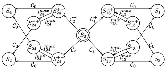
Figure 3. Supervisor. The active fault isolation is undertaken during $S_{13}^{++},S_{13}^{+-},S_{13}^{-+},S_{13}^{--},S_{24}^{++},S_{24}^{+-},$$S_{24}^{-+},S_{24}^{--}$. The events which triggers the active fault isolation are ${\mathcal{C}}_1^{+},{\mathcal{C}}_1^{-},{\mathcal{C}}_2^{+},{\mathcal{C}}_2^{-}$, while the only event which ends it is ${\mathcal{C}}_0$.

Remark 21.

The override signals let the related reference $l_{ni}\left(t\right)$ be piece-wise continuous, with piece-wise constant derivative (i.e., piece-wise constant speed). Moreover, $l_{ni}(t+T)=l_{max}$ (resp. $l_{ni}(t+T)=l_{min}$) is achieved in case of increasing (resp. decreasing) signal.

Remark 22.

The isolation is ideally achieved by the evaluation of the non-zero values of $r_1^{+}\left(t\right)$, $r_1^{-}\left(t\right)$, $r_2^{+}\left(t\right)$, $r_2^{-}\left(t\right)$. However, for robustness issues, a threshold-based evaluation is considered. More precisely, two thresholds are actually set, a first one denoted $t_{h_1}>0$ is considered during $S_0,S_1,S_2,S_3,S_4$ (i.e., when no active isolation is achieved), while a second threshold $t_{h_2}>0$ is considered for the remaining states (i.e., during the active isolation). In order to avoid high-frequency triggering events, we set $t_{h_1}>t_{h_2}$. The difference $t_{h_1}-t_{h_2}$, together with $t_{h_1}$ and $t_{h_2}$ themselves is a trade off between the robustness, the false negative/positive triggering events, and final estimation error of the stuck arm.

Remark 23.

The supervisor should be able to trigger whenever an event occurs. However, due to the noise, the residuals $r_1^{+}\left(t\right),r_1^{-}\left(t\right),r_2^{+}\left(t\right),r_2^{-}\left(t\right)$ can pass the thresholds (up and down) with high frequency, causing high rate triggering events. Then, once a transition to a new state is achieved, a minimum time $t_{min}>0$ is waited before the evaluation of any event. Formally, we could model this by adding a new (temporized) condition

$$o{k}_{t_{min}}=\left\{\begin{array}{cc}true\hfill & \mathit{if}\mathit{the}\mathit{current}\mathit{state}\mathit{is}\mathit{active}\mathit{for}\mathit{at}\mathit{least}{t}_{min}\mathit{seconds},\hfill \\ false\hfill & \mathit{otherwise}.\hfill \end{array}\right.$$

(86)

Then, each event $e\in E$ is replaced with the new one

$$e^{\prime }=e\mathit{and}o{k}_{t_{min}}.$$

(87)

Remark 24.

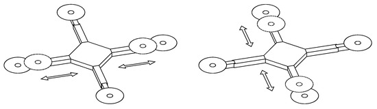
Figure 4 represents the graphical point of view about the active isolation and stuck estimation. Based on the isolated fault class (${\mathcal{C}}_1^{+},{\mathcal{C}}_1^{-},{\mathcal{C}}_2^{+},{\mathcal{C}}_2^{-}$), the supervisor starts to provide increasing or decreasing nominal arm lengths of the involved pair. The procedure stops when all the residual components are under the threshold. As it can be seen in Figure 3, livelocks are, however, possible. Then, a correct evaluation of the thresholds and the residual generator gains $H_1,H_2,H_3,H_4$ is needed.

Figure 4. During the active fault isolation (and estimation), both the arms in the isolated axis are increased/decreased.

Remark 25.

The overall active isolation procedure does not affect $u\left(t\right)$ (directly). Then, there is no need to stop the system motion or force hovering.

5. Fault-Tolerant DOBC Control

The feedback linearization fault-tolerant tracking controller is based on [25], where a DOBC approach is adopted for wind estimation and compensation [21].

Remark 26

(Disturbance observer). Let ${\tilde{F}}_w^E\left(t\right)=F_w^E\left(t\right)-{\widehat{F}}_w^E\left(t\right)$ be the estimation error. The disturbance observer

$${\Sigma }_{DO}:\begin{array}{cc}\hfill \dot{s}& =-Hs-H(\Phi +H{\dot{p}}_F)\hfill \\ \hfill {\widehat{F}}_w^E& =ms+mH{\dot{p}}_F,\hfill \end{array}$$

(88)

where $-H\in {\mathbb{R}}^{3\times 3}$ is a Hurwitz matrix and

$$\begin{array}{cc}\hfill \Phi & =-R_B^{E}S\left(r_G^B\right)J^{-1}S\left(\omega \right)J\omega -R_B^E{S}^2\left(\omega \right)r_G^B+g{e}_3+\frac{1}{m}{f}_z{R}_B^E{e}_3+R_B^{E}S\left(r_G^B\right)J^{-1}{M}_m^B,\hfill \end{array}$$

(89)

makes the estimation error dynamics

$$\begin{array}{cc}\hfill {\dot{\tilde{F}}}_w^E& =-H{\tilde{F}}_w^E+{\dot{F}}_w^E,\hfill \end{array}$$

(90)

which is a bounded input bounded output linear time-invariant system (with respect to ${\dot{F}}_w^E=0$) (see [25] for details).

Remark 27

(Inner loop). Let $v\left(t\right)=\mathrm{col}(v_z\left(t\right),v_{\eta }\left(t\right))$ be an auxiliary input, where $v_z\left(t\right)\in \mathbb{R}$ and $v_{\eta }\left(t\right)\in {\mathbb{R}}^3$. If ${\tilde{F}}_w^E\left(t\right)=0$, the regular static state feedback

$$u=F^{-1}{A}^{-1}(g(\omega ,\eta ,l)+v)$$

(91)

provides the input–output decoupling between $(z_F,\eta )$ and $(v_z,v_{\eta })$, where

$$\begin{array}{cc}\hfill g(\omega ,\eta ,l)& =\left[\begin{array}{c}-e_3^T(-R_B^{E}S\left(r_G^B\right)J^{-1}S\left(\omega \right)J\omega -R_B^E{S}^2\left(\omega \right)r_G^B+g{e}_3)-\frac{1}{m}{e}_3^T{\widehat{F}}_w^E\\ -(\dot{T}\left(\eta \right)\omega -T\left(\eta \right)J^{-1}S\left(\omega \right)J\omega )\end{array}\right],\hfill \end{array}$$

(92)

$$\begin{array}{cc}\hfill A& =\left[\begin{array}{cc}-\frac{1}{m}{e}_3^T{R}_B^E{e}_3& e_3^T{R}_B^{E}S\left(r_G^B\right)J^{-1}\\ 0& T\left(\eta \right)J^{-1}\end{array}\right].\hfill \end{array}$$

(93)

Moreover, let $z_{Fr}\left(t\right)\in \mathbb{R}$ and ${\eta }_r\left(t\right)=\mathrm{col}({\phi }_r\left(t\right),{\theta }_r\left(t\right),{\psi }_r\left(t\right))\in {\mathbb{R}}^3$ be the time varying reference signals for $z_F\left(t\right)$ and $\eta \left(t\right)$. The controls

$$\begin{array}{cc}\hfill v_z& ={\ddot{z}}_{Fr}-{\alpha }_{z1}({\dot{z}}_F-{\dot{z}}_{Fr})-{\alpha }_{z0}(z_F-z_{Fr}),\hfill \end{array}$$

(94)

$$\begin{array}{cc}\hfill v_{\eta }& ={\ddot{\eta }}_r-{\alpha }_{\eta 1}(T\left(\eta \right)\omega -{\dot{\eta }}_r)-{\alpha }_{\eta 0}(\eta -{\eta }_r),\hfill \end{array}$$

(95)

make the overall closed-loop error system bounded input bounded output with respect to ${\dot{F}}_w^E$ whenever the coefficients ${\alpha }_{z1},{\alpha }_{z0},{\alpha }_{\eta 1},{\alpha }_{\eta 0}$ solve the pole placement (see [25] for details).

Remark 28

(Outer loop). Let us assume near hovering conditions (i.e., $\phi \left(t\right)\approx \theta \left(t\right)\approx 0$) and let $e_x\left(t\right)=x_F\left(t\right)-x_{Fr}\left(t\right)$ and $e_y\left(t\right)=y_F\left(t\right)-y_{Fr}\left(t\right)$ be the error variables between $x_F\left(t\right)$ and $y_F\left(t\right)$ and their references $x_{Fr}\left(t\right)$ and $y_{Fr}\left(t\right)$. The control law

$$\left[\begin{array}{c}{\phi }_r\\ {\theta }_r\end{array}\right]=\frac{m}{f_z}\left[\begin{array}{cc}{s}_{\psi }& -c_{\psi }\\ c_{\psi }& s_{\psi }\end{array}\right]\left(-\left[\begin{array}{c}{e}_1^T\\ e_2^T\end{array}\right](\Gamma +\frac{1}{m}{\widehat{F}}_w^E)+\left[\begin{array}{c}{v}_x\\ v_y\end{array}\right]\right),$$

(96)

where

$$\begin{array}{cc}\hfill \Gamma & =-R_B^{E}S\left(r_G^B\right)J^{-1}S\left(\omega \right)J\omega -R_B^E{S}^2\left(\omega \right)r_G^B+g{e}_3+R_B^{E}S\left(r_G^B\right)J^{-1}{M}_m^B,\hfill \end{array}$$

(97)

$$\begin{array}{cccccccccccccccccc}\hfill {\tau }_x& ={\ddot{x}}_{Fr}-{\alpha }_{x1}({\dot{x}}_F-{\dot{x}}_{Fr})-{\alpha }_{x0}(x_F-x_F),\hfill & & & & & & & & & & & & & & & & \end{array}$$

(98)

$$\begin{array}{cccccccccccccccccc}\hfill {\tau }_y& ={\ddot{y}}_{Fr}-{\alpha }_{y1}({\dot{y}}_F-{\dot{y}}_{Fr})-{\alpha }_{y0}(y_F-y_F),\hfill & & & & & & & & & & & & & & & & \end{array}$$

(99)

forces the tracking error dynamics

$$\begin{array}{cc}\hfill {\ddot{e}}_x+{\alpha }_{x1}{\dot{e}}_x+{\alpha }_{x0}{e}_x& \approx e_1^T{\tilde{F}}_w\hfill \end{array}$$

(100)

$$\begin{array}{cc}\hfill {\ddot{e}}_y+{\alpha }_{y1}{\dot{e}}_y+{\alpha }_{y0}{e}_y& \approx e_2^T{\tilde{F}}_w.\hfill \end{array}$$

(101)

The coefficients ${\alpha }_{x1},{\alpha }_{x0},{\alpha }_{y1},{\alpha }_{y0}$ are then chosen according to a pole placement (see [25] for details).

The overall control scheme is reported in Figure 5.

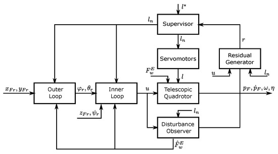
Figure 5. Control scheme. The vector $l^{★}$ describes the optimal/desired arm lengths provided by external software (e.g., an onboard artificial intelligence or a planning algorithm). Based on the residue $r=\mathrm{col}(r_1^{+},r_1^{-},r_2^{+},r_2^{-})$, the supervisor detects/isolates/identificates a fault (${\overline{l}}_i$), and eventually overrides $l^{★}$ with a new reference $l_n$. Based on a stuck fault in the servomotors, the actual arm lengths l could differ from $l_n$.

6. Numerical Simulations

The solution is tested in simulation using MATLAB under the following settings.

• Frequencies. The simulation is carried out for a total of 30 s. According to the double-loop structure, faster inner loop dynamics are achieved by both control parameters and different sample times. This solution takes into consideration computational limitations on a future implementation. In particular, the inner loop is simulated at 1 kHz, while the outer loop runs at 10 Hz. A zero order hold is applied for ${\phi }_r\left(t\right)$ and ${\theta }_r\left(t\right)$ between consecutive samples.
• Plant parameters. The frame and fixed arms are those of a DJI Flamewheel 450, the telescopic arms are of the same size and mass as the fixed ones, and the electric motors are the T-Motor AirGear 350. Table 3 summarizes the geometric dimensions and the dynamic parameters.
  Table 3. Geometric dimensions, dynamical parameters, and control parameters (see [29] for lift and drag coefficients).

  Parameters	Variables	Value	Unit
  Frame width and length	$w_0,l_0$	$0.1$	(m)
  Frame height	$h_0$	$0.5$	(m)
  Fixed and telescopic arm widths	$w_{i,j}$ ($i\le 4$, $j\le 2$)	$0.2$	(m)
  Fixed and telescopic arm lengths	$l_{i,j}$ ($i\le 4$, $j\le 2$)	$0.025$	(m)
  Motor radius	$r_{i,3}$ ($i\le 4$)	$0.012$	(m)
  Rotor radius	$r_{i,4}$ ($i\le 4$)	$0.12$	(m)
  Fixed and telescopic arms heights	$h_{i,j}$ ($i\le 4$, $j\le 2$)	$0.01$	(m)
  Motor heights	$h_{i,3}$ ($i\le 4$)	$0.03$	(m)
  Rotor heights	$h_{i,4}$ ($i\le 4$)	$0.003$	(m)
  Minimum arm length	$l_{min}$	$0.2$	(m)
  Maximum arm length	$l_{max}$	$0.4$	(m)
  Frame mass	$m_0$	$0.8$	(kg)
  Fixed and telescopic arm masses	$m_{i,j}$ ($i\le 4$, $j\le 2$)	$0.05$	(kg)
  Motor masses	$m_{i,3}$ ($i\le 4$)	$0.054$	(kg)
  Rotor masses	$m_{i,4}$ ($i\le 4$)	$0.008$	(kg)
  Total system mass	m	$1.448$	(kg)
  Gravitational acceleration	g	$9.81$	(m/s${}^2$)
  Linear friction coefficient	$k_t$	${10}^{-3}$	(N·s/m)
  Angular friction coefficient	$k_r$	${10}^{-2}$	(N·s·m)
  Lift coefficient	$c_L$	$3.13·{10}^{-5}$	(N·s${}^2$)
  Drag coefficient	$c_D$	$7.5·{10}^{-7}$	(N· m$·{\mathrm{s}}^2$)
  Inner loop frequency		${10}^3$	(Hz)
  Outer loop frequency		10	(Hz)
  Control input lower saturation		0	(N)
  Control input upper saturation		9	(N)
  $x_F$ and $y_F$ closed loop poles		$-1,-2$	$(-)$
  $z_F$ closed loop poles		$-1,-2$	$(-)$
  $\phi$ and $\theta$ closed loop poles		$-10,-20$	$(-)$
  $\psi$ closed loop poles		$-1,-2$	$(-)$
  Residual generator gains	$H_1,H_2$	10	$(-)$
  Observer gain	H	$4I$	$(-)$
  Threshold 1	$t_{h_1}$	10	$(-)$
  Threshold 2	$t_{h_2}$	3	$(-)$
  Minimum time for each state	$t_{min}$	1	(s)

• Sensors and Inertial Measurement Unit (IMU). The commonly adopted MPU-9250 IMU [28] is taken into consideration. Additive white Gaussian noise is applied to accelerations and gyroscopes, with standard deviation $7.8480·{10}^{-2}$ and $5.5192·{10}^{-3}$, respectively. Finally, due to Kalman filtering, a smaller noise is assumed for simplicity on attitude, linear velocity, and linear position (i.e., $2.7596·{10}^{-3}$, $1.5696·{10}^{-2}$, $7.8480·{10}^{-3}$, respectively).
• Input saturation. A saturation $0\le f_i\left(t\right)\le 9N$ is considered for each actual lift force. The total mass of the system is 1.448 kg, resulting in a thrust-to-weight ratio equal to $2.5$.
• Control parameters. All the control parameters have been heuristically set. The parameters for both the control law and the observer are summarized in Table 3.

In the following, four scenarios are simulated using the same tracking reference and the same control law parameters.

6.1. Scenario 1

A stuck fault on $l_1$ is injected at $t=10$ s, meanwhile, all the arm lengths commands $l_i^{★}\left(t\right)$ are decreasing after the fault injection. The overall demanded trajectory is an ascending helix for the first half of the simulation, and a descending helix for the second half of the simulation, as shown in Figure 6. The yaw angle is always kept at zero (i.e., ${\psi }_r\left(t\right)\equiv 0$).

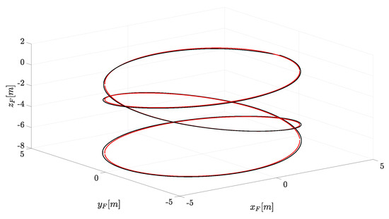
Figure 6. Trajectory of $p_F\left(t\right)$. The red plot represents the reference, while the black one represents the actual position.

The tracking performances of the linear positions and the yaw angle are reported in Figure 7. Linear position tracking errors are negligible, and the error on the yaw angle $\psi$ is acceptable: such error magnitude is up to $0.1$ rad, and this is a consequence of the chosen control law parameters.

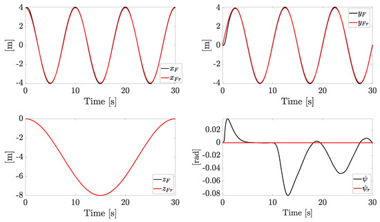
Figure 7. Tracking of $x_F\left(t\right)$, $y_F\left(t\right)$, $z_F\left(t\right)$ and $\psi \left(t\right)$.

The roll and pitch are reported in Figure 8. The effect of the zero-order hold is visible since the references are step-wise signals. The inner loop is able to achieve the goal, almost reaching the reference components before the successive sample time.

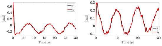
Figure 8. Tracking of $\phi \left(t\right)$ and $\theta \left(t\right)$. The reference signals are provided by the outer loop, which runs at a lower frequency. A zero-order hold is used between consecutive samples.

The actual wind components and their estimations are reported in Figure 9. The disturbance observer is slower than the disturbance (due to the bandwidth of the observer), but it is able to provide a good estimation. Indeed, tracking is achieved with no displacement due to wind.

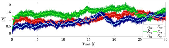
Figure 9. Wind components and their estimations.

The overall control inputs are reported in Figure 10. The saturation constraints are always matched.

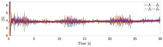
Figure 10. Control inputs.

Let us now compare the active isolation and diagnosis for the simulated scenarios. Actual arm lengths, estimations, and residues are plotted in Figure 11. Each arm starts with its maximum extension, while a shrinking phase on each arm is demanded starting from $t=10$ s. The first arm is stuck, hence the decreasing desired arm length leads to $s_{o1}\left(t\right)>0$, and the triggering of $r_1^{+}\left(t\right)>0$. The supervisor enters the active isolation phase (state $S_{13}^{++}$, precisely) and overrides the arm length command for the pair $(1,3)$. During the increase of $l_{n1}\left(t\right)$ and $l_{n3}\left(t\right)$ the residue $r_1^{+}\left(t\right)$ decreases (while the remaining residues are approximately null), hence when $r_1^{+}\left(t\right)\le t_{h_2}$ the event ${\mathcal{C}}_0$ triggers. The correct isolation is then achieved, together with an estimation of the stuck ${\overline{l}}_1$. The isolation is quite fast since the state $S_{13}^{++}$ directly moves the commanded signals toward the actual stuck arm length.

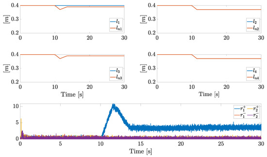
Figure 11. Actual arm lengths, nominal arm lengths, and residual components in Scenario 1.

6.2. Scenario 2

In this scenario, each arm starts with its minimum extension, while an enlarging phase on each arm is demanded starting from $t=10$ s. A stuck fault on $l_1$ is injected at $t=10$ s. Plots about fault isolation are summarized in Figure 12, while the plots about tracking performances will be not analyzed, as they are close to those of the first scenario. The stuck leads to $r_1^{-}\left(t\right)>0$ (in practice, $r_1^{-}\left(t\right)>t_{h_1}$), hence the supervisor enters the active fault isolation phase (state $S_{13}^{+-}$, precisely). The demanded arm lengths $l_{n1}^{★}\left(t\right)$ and $l_{n3}^{★}\left(t\right)$ are then again overrided with increasing signals. However, during this phase, the residues $r_1^{-}\left(t\right)$ will increase. When both $l_{n1}\left(t\right)$ and $l_{n_2}\left(t\right)$ reach the maximum length, the supervisor state transition to $S_{13}^{--}$ happens, leading to decreasing references. Finally, as $l_{n1}\left(t\right)$ approaches to ${\overline{l}}_1$, the residue decreases, until $r_1^{-}\left(t\right)<t_{h_2}$. Then, the events ${\mathcal{C}}_0$ triggers, the first arm is isolated as stuck and the actual arm length is estimated.

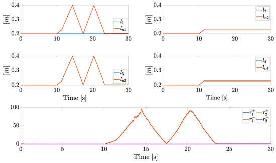
Figure 12. Actual arm lengths, nominal arm lengths, and residual components in Scenario 2.

6.3. Scenario 3

In this scenario, each arm starts with its maximum extension, while a shrinking phase on each arm is demanded starting from $t=10$ s. A stuck fault on $l_3$ is injected at $t=10$ s. From the isolation and identification point of view, this scenario is interesting: even if the stuck fault is on the third arm, the same fault class of Scenario 2 needs to be isolated by the residual generator, while the final result provided by the active fault isolation is expected to be different. Plots about fault isolation are summarized in Figure 13, while the plots about tracking performances will be not analyzed, as they are close to those of the earlier scenarios. The supervisor detects a fault and isolates the fault class ${\mathcal{C}}_1^{+}$. Differently from the Scenario 2, the supervisor policy is now an optimal one: by shrinking each arm, the triggered residue suddenly decreases, the scenario is isolated in less time, and fault isolation is achieved through the states sequence $S_0,S_{13}^{+-},S_3$ (the minimum number of transitions).

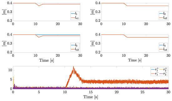
Figure 13. Actual arm lengths, nominal arm lengths, and residual components in Scenario 3.

6.4. Scenario 4

Finally, we consider a scenario where each arm starts with its minimum extension, while an enlarging phase on each arm is demanded starting from $t=10$ s. From the isolation and identification point of view, this scenario is the symmetric counterpart of Scenario 1. Plots about fault isolation are summarized in Figure 14, while the plots about tracking performances will be not analyzed, as they are close to those of the earlier scenarios. The overall isolation is accomplished through the state sequence $S_0,S_{13}^{++},S_{13}^{-+},S_3$. The active policy demands an enlarging phase, which does not lead to a residue reduction: the transition to $S_{13}^{-+}$ (shrinking phase) is required for the goal. The supervisor policy is not optimal, but isolation and identification are achieved, and no stability issues arise during the active isolation.

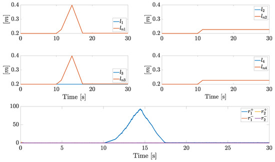
Figure 14. Actual arm lengths, nominal arm lengths, and residual components in Scenario 4.

7. Conclusions

The fault tolerant control of a telescopic quadrotor has been discussed. The fault diagnosis problem has been faced for servo motor stuck faults by exploiting the system symmetries. A residual generator provides the isolation into four fault classes, which in turn triggers an active fault isolation/identification phase, which finally solves the problem without constraining the lift forces. Indeed, such an active policy is handled by the supervisor, which has the main role of directly providing increasing/decreasing arm reference signals, ending the diagnosis. The wind is also taken into account and managed through a DOBC approach. The proposed solution is finally tested in simulation, where it can be seen how the goal is reached even under noise, actuators saturation, and model approximation.

Among the possible limitations which still affect the solution, we mention how the scheme is designed under the assumption of stuck faults only. Then, distinguishing between propeller faults and stuck servo faults is a future work, as well as extending the morphing degree of freedoms, and, finally, a hardware implementation of the solution.

Appendix A.1. Proof of Remark 9

For compactness, consider the functions

$$\begin{array}{cccc}\hfill c_x\left(\delta \right)& =\frac{cos\left(\delta \right)}{|cos(\delta \left)\right|},\hfill & \hfill c_y\left(\delta \right)& =\frac{sin\left(\delta \right)}{|sin(\delta \left)\right|},\hfill \end{array}$$

(A1)

where $\delta \ne k\frac{\pi }{2}$. For the symmetry of the rigid body $B_0\cup B_{1,1}\cup B_{1,2}\cup B_{1,3}\cup B_{1,4}$, we have $r_{1,1}^B=-r_{3,1}^B$, $r_{2,1}^B=-r_{4,1}^B$ and $m_{1,1}=m_{2,1}=m_{3,1}=m_{4,1}$. Moreover, $r_0^B=0$, hence

$$\begin{array}{c}\hfill \frac{1}{m}\left(m_0{r}_0^B+\sum _{i=1}^4{m}_{i,1}{r}_{i,1}^B\right)=0.\end{array}$$

(A2)

Additionally, we have $R_{1,1}^B{e}_1=-R_{1,3}^B{e}_1$ and $R_{2,1}^B{e}_1=-R_{3,3}^B{e}_1$. For each arm i, we have

$$\begin{array}{cc}\hfill r_{i,4}^B& =r_{i,3}^B=c_x\left({\delta }_i\right)\frac{w_0}{2}{e}_1+c_y\left({\delta }_i\right)\frac{l_0}{2}{e}_2+l_i{R}_{i,1}^B{e}_1,\hfill \end{array}$$

(A3)

$$\begin{array}{cccccccccccccccc}\hfill r_{i,2}^B& =r_{i,4}^B-\frac{w_{i,2}}{2}{R}_{i,1}^B{e}_1,\hfill & & & & & & & & & & & & & & \end{array}$$

(A4)

hence

$$\begin{array}{cc}\hfill \sum _{i=1}^4{r}_{i,4}^B=\sum _{i=1}^4{r}_{i,3}^B& =\sum _{i=1}^4{c}_x\left({\delta }_i\right)\frac{w_0}{2}{e}_1+\sum _{i=1}^4{c}_y\left({\delta }_i\right)\frac{l_0}{2}{e}_2+\sum _{i=1}^4{l}_i{R}_{i,1}^B{e}_1\hfill \end{array}$$

(A5)

$$\begin{array}{cc}\hfill & =\sum _{i=1}^4{l}_i{R}_{i,1}^B{e}_1,\hfill \end{array}$$

(A6)

$$\begin{array}{cc}\hfill \sum _{i=1}^4{r}_{i,2}^B& =\sum _{i=1}^4{r}_{i,4}^B-\sum _{i=1}^4\frac{w_{i,2}}{2}{R}_{i,1}^B{e}_1\hfill \end{array}$$

(A7)

$$\begin{array}{cc}\hfill & =\sum _{i=1}^4{r}_{i,4}^B-4\frac{w_{1,2}}{2}\sum _{i=1}^4{R}_{i,1}^B{e}_1\hfill \end{array}$$

(A8)

$$\begin{array}{cc}\hfill & =\sum _{i=1}^4{r}_{i,4}^B.\hfill \end{array}$$

(A9)

Finally,

$$\begin{array}{cc}\hfill r_G^B& =\frac{1}{m}\left(m_0{r}_0^B+\sum _{i=1}^4\sum _{j=1}^4{m}_{i,j}{r}_{i,j}^B\right)\hfill \end{array}$$

(A10)

$$\begin{array}{cc}\hfill & =\frac{1}{m}\left(m_0{r}_0^B+\sum _{i=1}^4{m}_{i,1}{r}_{i,1}^B\right)+\frac{1}{m}\sum _{i=1}^4\sum _{j=2}^4{m}_{i,j}{r}_{i,j}^B\hfill \end{array}$$

(A11)

$$\begin{array}{cc}\hfill & =\frac{1}{m}\left(\sum _{i=1}^4{m}_{i,2}{r}_{i,2}^B+\sum _{i=1}^4{m}_{i,3}{r}_{i,3}^B+\sum _{i=1}^4{m}_{i,4}{r}_{i,4}^B\right)\hfill \end{array}$$

(A12)

$$\begin{array}{cc}\hfill & =\frac{1}{m}\left(m_{1,2}\sum _{i=1}^4{r}_{i,2}^B+m_{1,3}\sum _{i=1}^4{r}_{i,3}^B+m_{1,4}\sum _{i=1}^4{r}_{i,4}^B\right)\hfill \end{array}$$

(A13)

$$\begin{array}{c}=\frac{m_{1,2}+m_{1,3}+m_{1,4}}{m}\sum _{i=1}^4{r}_{i,4}^B\hfill \end{array}$$

(A14)

$$\begin{array}{cc}\hfill & =\frac{m_{1,2}+m_{1,3}+m_{1,4}}{m}\sum _{i=1}^4{l}_i{R}_{i,1}^B{e}_1\hfill \end{array}$$

(A15)

$$\begin{array}{cc}\hfill & =K_{G}l,\hfill \end{array}$$

(A16)

where, in the last step, it is noted that $K_G$ can be rewritten as

$$K_G=\frac{m_{1,2}+m_{1,3}+m_{1,4}}{m}\left[\begin{array}{cccc}{R}_{1,1}^B{e}_1& R_{2,1}^B{e}_1& R_{3,1}^B{e}_1& R_{4,1}^B{e}_1\end{array}\right],$$

(A17)

or, in a matrix fashion, as

$$K_G=\frac{m_{1,2}+m_{1,3}+m_{1,4}}{m}\left[\begin{array}{cccc}cos\left({\delta }_1\right)& cos\left({\delta }_2\right)& cos\left({\delta }_3\right)& cos\left({\delta }_4\right)\\ sin\left({\delta }_1\right)& sin\left({\delta }_2\right)& sin\left({\delta }_3\right)& sin\left({\delta }_4\right)\\ 0& 0& 0& 0\end{array}\right].$$

(A18)

Appendix A.2. Proof of Remark 10

First, note that

$$\left(R_{i,1}^B{e}_1\right)\times e_3=-R_{i,1}^B(e_3\times e_1)=-R_{i,1}^B{e}_2.$$

(A19)

We have

$$\begin{array}{cc}\hfill -\sum _{i=1}^4{r}_{i,4}^B{f}_i\times e_3& =-\sum _{i=1}^4{f}_i\left(c_x\left({\delta }_i\right)\frac{w_0}{2}{e}_1+c_y\left({\delta }_i\right)\frac{l_0}{2}{e}_2\right)\times e_3-\sum _{i=1}^4{f}_i{l}_i{R}_{i,1}^B{e}_1\times e_3\hfill \end{array}$$

(A20)

$$\begin{array}{cccccc}& & & & & =-\sum _{i=1}^4{f}_i\left(c_y\left({\delta }_i\right)\frac{l_0}{2}{e}_1-c_x\left({\delta }_i\right)\frac{w_0}{2}{e}_2\right)+\sum _{i=1}^4{f}_i{l}_i{R}_{i,1}^B{e}_2\hfill \end{array}$$

(A21)

and

$$\begin{array}{cc}\hfill \sum _{i=1}^4{r}_G^B\times f_i{e}_3& =\left(\sum _{i=1}^4{f}_i\right)r_G^B\times e_3=-\left(\sum _{i=1}^4{f}_i\right)S_3{K}_{G}l.\hfill \end{array}$$

(A22)

The thrust torque is

$$\begin{array}{cc}\hfill M_{thrust}^B& =-\sum _{i=1}^4\left((r_{i,4}^B-r_G^B)\times f_i{e}_3\right)\hfill \end{array}$$

(A23)

$$\begin{array}{cc}\hfill & =-\sum _{i=1}^4\left(f_i{r}_{i,4}^B\right)\times e_3+\sum _{i=1}^4{r}_G^B\times f_i{e}_3\hfill \end{array}$$

(A24)

$$\begin{array}{cc}\hfill & =-\sum _{i=1}^4{f}_i\left(c_y\left({\delta }_i\right)\frac{l_0}{2}{e}_1-c_x\left({\delta }_i\right)\frac{w_0}{2}{e}_2\right)+\sum _{i=1}^4{f}_i{l}_i{R}_{i,1}^B{e}_2-\left(\sum _{i=1}^4{f}_i\right)S_3{K}_{G}l,\hfill \end{array}$$

(A25)

and, considering that $M_m^B=M_{drag}^B+M_{torque}^B$, we have $M_m^B=v+K_{m}l$, where

$$\begin{array}{cc}\hfill v& =\sum _{i=1}^4{c}_{w_i}\frac{c_D}{c_L}{f}_i-\sum _{i=1}^4{f}_i\left(c_y\left({\delta }_i\right)\frac{l_0}{2}{e}_1-c_x\left({\delta }_i\right)\frac{w_0}{2}{e}_2\right)\hfill \end{array}$$

(A26)

$$\begin{array}{cc}\hfill & =\sum _{i=1}^4{f}_i\left(c_{w_i}\frac{c_D}{c_L}{e}_3-c_y\left({\delta }_i\right)\frac{l_0}{2}{e}_1+c_x\left({\delta }_i\right)\frac{w_0}{2}{e}_2\right)\hfill \end{array}$$

(A27)

$$\begin{array}{cc}\hfill & =K_{v}u,\hfill \end{array}$$

(A28)

and

$$\begin{array}{cc}\hfill K_m& =\left[\begin{array}{cccc}{f}_1{R}_{11}^B{e}_2& f_2{R}_{21}^B{e}_2& f_3{R}_{31}^B{e}_2& f_4{R}_{41}^B{e}_2\end{array}\right]-\left(\sum _{i=1}^4{f}_i\right)S_3{K}_G.\hfill \end{array}$$

(A29)

It is indeed noted that $K_v$ can be rewritten in a matrix fashion as

$$K_v=\left[\begin{array}{cccc}-c_y\left({\delta }_1\right)\frac{l_0}{2}& -c_y\left({\delta }_2\right)\frac{l_0}{2}& -c_y\left({\delta }_3\right)\frac{l_0}{2}& -c_y\left({\delta }_4\right)\frac{l_0}{2}\\ c_x\left({\delta }_1\right)\frac{w_0}{2}& c_x\left({\delta }_2\right)\frac{w_0}{2}& c_x\left({\delta }_3\right)\frac{w_0}{2}& c_x\left({\delta }_4\right)\frac{w_0}{2}\\ c_{w_1}\frac{c_D}{c_L}& c_{w_2}\frac{c_D}{c_L}& c_{w_3}\frac{c_D}{c_L}& c_{w_4}\frac{c_D}{c_L}\end{array}\right].$$

(A30)

For $i=1,\dots ,4$, we have

$$f_i{R}_{i,1}^B{e}_2=R_{i,1}^B{E}_{2,1}u$$

(A31)

and

$$\begin{array}{cc}\hfill \left(\sum _{j=1}^4{f}_j\right)R_{i,1}^B{e}_2& =\left(\sum _{j=1}^4{f}_j{R}_{i,1}^B{e}_2\right)\hfill \end{array}$$

(A32)

$$\begin{array}{cc}\hfill & =\left[\begin{array}{cccc}{R}_{i,1}^B{e}_2& R_{i,1}^B{e}_2& R_{i,1}^B{e}_2& R_{i,1}^B{e}_2\end{array}\right]u\hfill \end{array}$$

(A33)

$$\begin{array}{cc}\hfill & =R_{i,1}^B(E_{2,1}+E_{2,2}+E_{2,3}+E_{2,4})u.\hfill \end{array}$$

(A34)

Finally, the i-th column of $K_m\left(u\right)$ is

$$\begin{array}{cc}\hfill K_m^i\left(u\right)& =f_i{R}_{i,1}^B{e}_2-\frac{m_{1,2}+m_{1,3}+m_{1,4}}{m}\left(\sum _{j=1}^4{f}_j\right)S_3{R}_{i,1}^B{e}_1\hfill \end{array}$$

(A35)

$$\begin{array}{cc}\hfill & =f_i{R}_{i,1}^B{e}_2-\frac{m_{1,2}+m_{1,3}+m_{1,4}}{m}\left(\sum _{j=1}^4{f}_j\right)R_{i,1}^B{e}_2\hfill \end{array}$$

(A36)

$$\begin{array}{cc}\hfill & =R_{i,1}^B{E}_{2,i}u-\frac{m_{1,2}+m_{1,3}+m_{1,4}}{m}{R}_{i,1}^B(E_{2,1}+E_{2,2}+E_{2,3}+E_{2,4})u\hfill \end{array}$$

(A37)

$$\begin{array}{cc}\hfill & =D_{i}u.\hfill \end{array}$$

(A38)

References

- Pütsep, K.; Rassõlkin, A. Methodology for Flight Controllers for Nano, Micro and Mini Drones Classification. In Proceedings of the 2021 International Conference on Engineering and Emerging Technologies (ICEET), Istanbul, Turkey, 27–28 October 2021; pp. 1–8. [Google Scholar] [CrossRef]
- Longhi, M.; Taylor, Z.; Popović, M.; Nieto, J.; Marrocco, G.; Siegwart, R. RFID-Based Localization for Greenhouses Monitoring Using MAVs. In Proceedings of the 2018 IEEE-APS Topical Conference on Antennas and Propagation in Wireless Communications (APWC), Columbia, SC, USA, 10–14 September 2018; pp. 905–908. [Google Scholar] [CrossRef]
- Cutler, M.; How, J.P. Analysis and control of a variable-pitch quadrotor for agile flight. J. Dyn. Syst. Meas. Control 2015, 137, 101002. [Google Scholar] [CrossRef]
- Niemiec, R.; Gandhi, F.; Lopez, M.; Tischler, M. System identification and handling qualities predictions of an eVTOL urban air mobility aircraft using modern flight control methods. In Proceedings of the Vertical Flight Society 76th Annual Forum, Virtual, 5–8 October 2020. [Google Scholar]
- Wang, Z.; Groß, R.; Zhao, S. Controllability analysis and controller design for variable-pitch propeller quadcopters with one propeller failure. Adv. Control. Appl. Eng. Ind. Syst. 2020, 2, e29. [Google Scholar] [CrossRef]
- Baldini, A.; Felicetti, R.; Freddi, A.; Longhi, S.; Monteriù, A. Actuator fault tolerant control of variable pitch quadrotor vehicles. IFAC-PapersOnLine 2020, 53, 4095–4102. [Google Scholar] [CrossRef]
- Tuna, T.; Ovur, S.E.; Gokbel, E.; Kumbasar, T. Design and development of FOLLY: A self-foldable and self-deployable quadcopter. Aerosp. Sci. Technol. 2020, 100, 105807. [Google Scholar] [CrossRef]
- Peraza-Hernandez, E.A.; Hartl, D.J.; Malak, R.J., Jr.; Lagoudas, D.C. Origami-inspired active structures: A synthesis and review. Smart Mater. Struct. 2014, 23, 094001. [Google Scholar] [CrossRef]
- Mintchev, S.; Floreano, D. A pocket sized foldable quadcopter for situational awareness and reconnaissance. In Proceedings of the 2016 IEEE International Symposium on Safety, Security, and Rescue Robotics (SSRR), Lausanne, Switzerland, 23–27 October 2016; pp. 396–401. [Google Scholar]
- Shu, J.; Chirarattananon, P. A quadrotor with an origami-inspired protective mechanism. IEEE Robot. Autom. Lett. 2019, 4, 3820–3827. [Google Scholar] [CrossRef]
- Avant, T.; Lee, U.; Katona, B.; Morgansen, K. Dynamics, hover configurations, and rotor failure restabilization of a morphing quadrotor. In Proceedings of the 2018 IEEE American Control Conference (ACC), Milwaukee, WI, USA, 27–28 June 2018; pp. 4855–4862. [Google Scholar]
- Brischetto, S.; Ciano, A.; Ferro, C.G. A multipurpose modular drone with adjustable arms produced via the FDM additive manufacturing process. Curved Layer. Struct. 2016, 3, 202–213. [Google Scholar] [CrossRef]
- Falanga, D.; Kleber, K.; Mintchev, S.; Floreano, D.; Scaramuzza, D. The foldable drone: A morphing quadrotor that can squeeze and fly. IEEE Robot. Autom. Lett. 2018, 4, 209–216. [Google Scholar] [CrossRef]
- Desbiez, A.; Expert, F.; Boyron, M.; Diperi, J.; Viollet, S.; Ruffier, F. X-Morf: A crash-separable quadrotor that morfs its X-geometry in flight. In Proceedings of the 2017 Workshop on Research, Education and Development of Unmanned Aerial Systems (RED-UAS), Linkoping, Sweden, 3–5 October 2017; pp. 222–227. [Google Scholar]
- Derrouaoui, S.; Guiatni, M.; Bouzid, Y.; Dib, I.; Moudjari, N. Dynamic modeling of a transformable quadrotor. In Proceedings of the 2020 International Conference on Unmanned Aircraft Systems (ICUAS), Athens, Greece, 1–4 September 2020; pp. 1714–1719. [Google Scholar]
- Zhao, M.; Kawasaki, K.; Chen, X.; Noda, S.; Okada, K.; Inaba, M. Whole-body aerial manipulation by transformable multirotor with two-dimensional multilinks. In Proceedings of the 2017 IEEE International Conference on Robotics and Automation (ICRA), Singapore, 29 May–3 June 2017; pp. 5175–5182. [Google Scholar]
- Pose, C.; Giribet, J. Multirotor fault tolerance based on center-of-mass shifting in case of rotor failure. In Proceedings of the 2021 International Conference on Unmanned Aircraft Systems (ICUAS), Athens, Greece, 15–18 June 2021; pp. 38–46. [Google Scholar]
- Kumar, R.; Deshpande, A.M.; Wells, J.Z.; Kumar, M. Flight control of sliding arm quadcopter with dynamic structural parameters. In Proceedings of the 2020 IEEE/RSJ International Conference on Intelligent Robots and Systems (IROS), Las Vegas, NV, USA, 24 October 2020–24 January 2021; pp. 1358–1363. [Google Scholar]
- Xu, C.; Yang, Z.; Zhang, Z.; Xu, H.; Wu, J.; Zhou, D.; Liao, L.; Zhang, Q. Design and Control of a Deformable Trees-Pruning Aerial Robot. Complexity 2020, 2020, 6627339. [Google Scholar] [CrossRef]
- Tomić, T.; Ott, C.; Haddadin, S. External wrench estimation, collision detection, and reflex reaction for flying robots. IEEE Trans. Robot. 2017, 33, 1467–1482. [Google Scholar] [CrossRef]
- Li, S.; Yang, J.; Chen, W.; Chen, X. Disturbance Observer-Based Control: Methods and Applications; CRC Press: Boca Raton, FL, USA; Taylor & Francis Group: Abingdon, UK, 2017. [Google Scholar]
- De Persis, C.; Isidori, A. A geometric approach to nonlinear fault detection and isolation. IEEE Trans. Autom. Control 2001, 46, 853–865. [Google Scholar] [CrossRef]
- Isermann, R. Fault-Diagnosis Systems: An Introduction from Fault Detection to Fault Tolerance; Springer: Berlin/Heidelberg, Germany, 2005. [Google Scholar]
- Chen, J.; Patton, R. Robust Model-Based Fault Diagnosis for Dynamic Systems; Springer: New York, NY, USA, 2012. [Google Scholar]
- Baldini, A.; Felicetti, R.; Freddi, A.; Longhi, S.; Monteriù, A. Modeling and Control of a Telescopic Quadrotor Using Disturbance Observer Based Control. In Proceedings of the 2022 30th Mediterranean Conference on Control and Automation (MED), Athens, Greece, 28 June–1 July 2022; pp. 396–402. [Google Scholar] [CrossRef]
- Fossen, T. Guidance and Control of Ocean Vehicles; Wiley: Hoboken, NJ, USA, 1994. [Google Scholar]
- Michieletto, G.; Ryll, M.; Franchi, A. Fundamental actuation properties of multirotors: Force–moment decoupling and fail–safe robustness. IEEE Trans. Robot. 2018, 34, 702–715. [Google Scholar] [CrossRef]
- TDK InvenSense. MPU-9250, Nine-Axis (Gyro + Accelerometer + Compass) MEMS MotionTracking™ Device. 2016. Available online: https://invensense.tdk.com/download-pdf/mpu-9250-datasheet/ (accessed on 24 March 2023).
- Becker, M.; Sampaio, R.C.B.; Bouabdallah, S.; Perrot, V.d.; Siegwart, R. In-flight collision avoidance controller based only on OS4 embedded sensors. J. Braz. Soc. Mech. Sci. Eng. 2012, 34, 294–307. [Google Scholar] [CrossRef]
Disclaimer/Publisher’s Note: The statements, opinions and data contained in all publications are solely those of the individual author(s) and contributor(s) and not of MDPI and/or the editor(s). MDPI and/or the editor(s) disclaim responsibility for any injury to people or property resulting from any ideas, methods, instructions or products referred to in the content. |
© 2023 by the authors. Licensee MDPI, Basel, Switzerland. This article is an open access article distributed under the terms and conditions of the Creative Commons Attribution (CC BY) license (https://creativecommons.org/licenses/by/4.0/).