Inertial Iterative Self-Adaptive Step Size Extragradient-Like Method for Solving Equilibrium Problems in Real Hilbert Space with Applications

Abstract

A number of applications from mathematical programmings, such as minimization problems, variational inequality problems and fixed point problems, can be written as equilibrium problems. Most of the schemes being used to solve this problem involve iterative methods, and for that reason, in this paper, we introduce a modified iterative method to solve equilibrium problems in real Hilbert space. This method can be seen as a modification of the paper titled “A new two-step proximal algorithm of solving the problem of equilibrium programming” by Lyashko et al. (Optimization and its applications in control and data sciences, Springer book pp. 315–325, 2016). A weak convergence result has been proven by considering the mild conditions on the cost bifunction. We have given the application of our results to solve variational inequality problems. A detailed numerical study on the Nash–Cournot electricity equilibrium model and other test problems is considered to verify the convergence result and its performance.

1. Introduction

An equilibrium problem (EP) is a generalized concept that unifies several mathematical problems, such as the variational inequality problems, minimization problems, complementarity problems, the fixed point problems, non-cooperative games of Nash equilibrium, the saddle point problems and scalar and vector minimization problems (see e.g., [1,2,3]). The particular form of an equilibrium problem was firstly established in 1992 by Muu and Oettli [4] and then further elaborated by Blum and Oettli [1]. Next, we consider the concept of an equilibrium problem introduced by Blum and Oettli in [1]. Let C be a non-empty, closed and convex subset $\mathbb{H}$ of a real Hilbert space and $f:\mathbb{H}\times \mathbb{H}\to \mathbb{R}$ is bifunction with $f(v,v)=0$, for each $v\in C.$ A equilibrium problem regarding f on the set C is defined in the following way:

$$\mathrm{Find}p\in C\mathrm{such}\mathrm{that}f(p,v)\ge 0,\mathrm{for}\mathrm{all}v\in C.$$

(1)

Many methods have been already established over the past couple of years to figure out the equilibrium problem in Hilbert spaces [5,6,7,8,9,10,11,12,13,14,15], the inertial methods [11,16,17,18] and others in [18,19,20,21,22,23,24]. In particular, Tran et al. introduced an iterative scheme in [8], in that a sequence $\left\{u_n\right\}$ was generated in the following way:

$$\left\{\begin{array}{c}{u}_0\in C,\hfill \\ v_n=argmin\{\lambda f(u_n,y)+\frac{1}{2}\parallel u_n-y{\parallel }^2:y\in C\},\hfill \\ u_{n+1}=argmin\{\lambda f(v_n,y)+\frac{1}{2}\parallel u_n-y{\parallel }^2:y\in C\},\hfill \end{array}\right.$$

(2)

where $0<\lambda <min\left\{\frac{1}{2c_1},\frac{1}{2c_2}\right\}$ and $c_1,c_2$ are Lipschitz constants. Lyashko et al. [25] in 2016 introduced an improvement of the method (2) to solve equilibrium problem and sequence $\left\{u_n\right\}$ was generated in the following way:

$$\left\{\begin{array}{c}{u}_0,v_0\in C,\hfill \\ u_{n+1}=argmin\{\lambda f(v_n,y)+\frac{1}{2}\parallel u_n-y{\parallel }^2:y\in C\},\hfill \\ v_{n+1}=argmin\{\lambda f(v_n,y)+\frac{1}{2}\parallel u_{n+1}-y{\parallel }^2:y\in C\},\hfill \end{array}\right.$$

(3)

where $0<\lambda <\frac{1}{2c_2+4c_1}$ and $c_1,c_2$ are Lipschitz constants.

In this paper, we consider the extragradient method in (3) and to provide its improvement by using the inertial scheme [26] and continue to improve the step size rule for its second step. The step size is not fixed in our case, but it is dependent on a particular formula by using prior information of the bifunction values. A weak convergence theorem dealing with the suggested technique is presented by having the specific bi-functional condition. We have also considered how our results are presented to the problems of a variational inequality. A few other formulations of the problem of variational inequalities are discussed, and many computational examples in finite and infinite dimensions spaces are also presented to demonstrate the applicability of our proposed results.

In this study, we study the equilibrium problem through the following assumptions:

($f_1$)

A bifunction $f:\mathbb{H}\times \mathbb{H}\to \mathbb{R}$ is said to be (see [1,27]) pseudomonotone on C if

$$f(v_1,v_2)\ge 0⟹f(v_2,v_1)\le 0,\mathrm{for}\mathrm{all}{v}_1,v_2\in C.$$

($f_2$)

A bifunction $f:\mathbb{H}\times \mathbb{H}\to \mathbb{R}$ is said to be Lipschitz-type continuous [28] on C if there exist $c_1,c_2>0$ such that

$$f(v_1,v_3)\le f(v_1,v_2)+f(v_2,v_3)+c_1\parallel v_1-v_2{\parallel }^2+c_2{\parallel v_2-v_3\parallel }^2,\mathrm{for}\mathrm{all}{v}_1,v_2,v_3\in C.$$

($f_3$)

$\underset{n\to +\infty }{lim\; sup}f(v_n,z)\le f(v^{*},z)$ for each $z\in C$ and $\left\{v_n\right\}\subset C$ satisfying $v_n\rightharpoonup v^{*};$

($f_4$)

$f(u,·)$ is convex and subdifferentiable on $\mathbb{H}$ for each $u\in \mathbb{H}.$

The rest of this paper will be organized as follows: In Section 2, we give a few definitions and important lemmas to be used in this paper. Section 3 includes the main algorithm involving pseudomonotone bifunction and provides a weak convergence theorem. Section 4 describes some applications in the variational inequality problems. Section 5 sets out the numerical studies to demonstrate the algorithmic efficiency.

2. Preliminaries

In this section, some important lemmas and basic definitions are provided. Moreover, $EP(f,C)$ denotes the solution set of an equilibrium problem on the set C and p is any arbitrary element of $EP(f,C)$.

A metric projection $P_C\left(u\right)$ of u onto a closed, convex subset C of $\mathbb{H}$ is defined by

$$P_C\left(u\right)=\underset{v\in C}{argmin}\{\parallel v-u\parallel \}.$$

Lemma 1

([29]). Let $P_C:\mathbb{H}\to C$ be a metric projection from $\mathbb{H}$ onto $C.$ Then

(i)

For all $u\in C,$$v\in \mathbb{H}$ and

$$\parallel u-P_C{\left(v\right)\parallel }^2+\parallel P_C{\left(v\right)-v\parallel }^2\le {\parallel u-v\parallel }^2.$$

(ii)

$w=P_C\left(u\right)$ if and only if

$$⟨u-w,v-w⟩\le 0,\mathrm{for}\mathrm{all}v\in C.$$

Lemma 2

([29]). For all $u,v\in \mathbb{H}$ with $\daleth \in \mathbb{R}$. Then, the following relationship is holds.

$${\parallel \daleth u+(1-\daleth )v\parallel }^2={\daleth \parallel u\parallel }^2+{(1-\daleth )\parallel v\parallel }^2-\daleth (1-\daleth ){\parallel u-v\parallel }^2.$$

Assume that $g:C\to \mathbb{R}$ be a convex function and subdifferential of g at $u\in C$ is defined by

$$\partial g\left(u\right)=\{w\in C:g(v)-g(u)\ge ⟨w,v-u⟩,\mathrm{for}\mathrm{all}v\in C\}.$$

Given that $f(u,.)$ is convex and subdifferentiable on $\mathbb{H}$ for each fixed $u\in \mathbb{H}$ and subdifferential of $f(u,.)$ at $x\in \mathbb{H}$ defined by

$${\partial }_{2}f(u,.)\left(x\right)={\partial }_{2}f(u,x)=\{z\in \mathbb{H}:f(u,v)-f(u,x)\ge ⟨z,v-x⟩,\mathrm{for}\mathrm{all}v\in \mathbb{H}\}.$$

A normal cone of C at $u\in C$ is defined by

$$N_C\left(u\right)=\{w\in \mathbb{H}:⟨w,v-u⟩\le 0,\mathrm{for}\mathrm{all}v\in C\}.$$

Lemma 3.

([30]). Assume that C is a nonempty, closed and convex subset of a real Hilbert space $\mathbb{H}$ and $h:C\to \mathbb{R}$ be a convex, lower semi-continuous and subdifferentiable function on $C.$ Then, $u\in C$ is a minimizer of a function h if and only if $0\in \partial h\left(u\right)+N_C\left(u\right)$ where $\partial h\left(u\right)$ and $N_C\left(u\right)$ denotes the subdifferential of h at u and the normal cone of C at u, respectively.

Lemma 4

([31]). Let $a_n$, $b_n$ and $c_n$ are non-negative real sequences such that

$$a_{n+1}\le a_n+b_n(a_n-a_{n-1})+c_n,\mathit{for}\mathit{all}n\ge 1,\mathit{with}\sum _{n=1}^{+\infty }{c}_n<+\infty ,$$

where $b>0$ such that $0\le b_n\le b<1$ for all $n\in \mathbb{N}.$ Then, the following relations are true.

(i)

${\displaystyle \sum _{n=1}^{+\infty }{[a_n-a_{n-1}]}_{+}<+\infty ,}$ with ${\left[s\right]}_{+}:=max\{s,0\};$

(ii)

${lim}_{n\to +\infty }{a}_n=a^{*}\in [0,+\infty ).$

Lemma 5

([32]). Let a sequence $\left\{a_n\right\}$ in $\mathbb{H}$ and $C\subset \mathbb{H}$ and the following conditions have been met:

(i)

for each $a\in C,$${lim}_{n\to +\infty }\parallel a_n-a\parallel$ exists;

(ii)

each weak sequentially limit point of $\left\{a_n\right\}$ belongs to set C.

Then, $\left\{a_n\right\}$ weakly converges to an element in $C.$

3. Main Results

In this section, we present our main algorithm and provide a weak convergence theorem for our proposed method. The detailed method is given below.

Remark 1.

By Expression (5), we obtain

$${\lambda }_{n+1}\left[f(v_{n-1},u_{n+1})-f(v_{n-1},v_n)-c_1\parallel v_{n-1}-v_n{\parallel }^2-c_2{\parallel v_n-u_{n+1}\parallel }^2\right]\le \mu f(v_n,u_{n+1}).$$

(4)

Lemma 6.

Let $\left\{u_n\right\}$ be a sequence generated by Algorithm 1. Then, the following inequality holds.

$$\mu {\lambda }_{n}f(v_n,y)-\mu {\lambda }_{n}f(v_n,u_{n+1})\ge ⟨{\rho }_n-u_{n+1},y-u_{n+1}⟩,\mathit{for}\mathit{all}y\in C.$$

Algorithm 1 Modified Popov’s subgradient extragradient-like iterative scheme.

Step 1: Choose $u_{-1},v_{-1},u_0,v_0\in \mathbb{H}$ and a sequence ${\wp }_n$ is non-decreasing such that $0\le {\wp }_n\le \wp <\frac{1}{3}$, ${\lambda }_0>0$ and $0<\sigma <min\left\{\frac{1-3\wp }{{(1-\wp )}^2+4c_1(\wp +{\wp }^2)},\frac{1}{2c_2+4c_1(1+\wp )}\right\}$ and $\mu \in (0,\sigma )$.   Step 2: Evaluate $$u_{n+1}=argmin\{\mu {\lambda }_{n}f(v_n,y)+\frac{1}{2}\parallel {\rho }_n-y{\parallel }^2:y\in C\},$$ where ${\rho }_n=u_n+{\wp }_n(u_n-u_{n-1}).$   Step 3: Updated the step size in the following order: $${\lambda }_{n+1}=\left\{\begin{array}{cc}min\left\{\sigma ,\frac{\mu f(v_n,u_{n+1})}{f(v_{n-1},u_{n+1})-f(v_{n-1},v_n)-c_1\parallel v_{n-1}-v_n{\parallel }^2-c_2{\parallel u_{n+1}-v_n\parallel }^2+1}\right\},\hfill & \\ \mathrm{if}\frac{\mu f(v_n,u_{n+1})}{f(v_{n-1},u_{n+1})-f(v_{n-1},v_n)-c_1\parallel v_{n-1}-v_n{\parallel }^2-c_2{\parallel u_{n+1}-v_n\parallel }^2+1}>0,\hfill & \\ {\lambda }_0\hfill & else.\hfill \end{array}\right.$$ (5)   Step 4: Evaluate $$v_{n+1}=argmin\{{\lambda }_{n+1}f(v_n,y)+\frac{1}{2}\parallel {\rho }_{n+1}-y{\parallel }^2:y\in C\},$$ where ${\rho }_{n+1}=u_{n+1}+{\wp }_{n+1}(u_{n+1}-u_n).$ If $u_{n+1}=v_n={\rho }_n$ or ${\rho }_{n+1}=v_{n+1}=v_n$ then Stop. Else, take $n:=n+1$ and go back to Step 2.

Proof. 

By the use of Lemma 3, we get

$$0\in {\partial }_2\left\{\mu {\lambda }_{n}f(v_n,y)+\frac{1}{2}{\parallel {\rho }_n-y\parallel }^2\right\}\left(u_{n+1}\right)+N_C\left(u_{n+1}\right).$$

From above there is a $\omega \in {\partial }_{2}f(v_n,u_{n+1})$ and $\overline{\omega }\in N_C\left(u_{n+1}\right)$ such that

$$\mu {\lambda }_n\omega +u_{n+1}-{\rho }_n+\overline{\omega }=0.$$

Therefore, we obtain

$$⟨{\rho }_n-u_{n+1},y-u_{n+1}⟩=\mu {\lambda }_n⟨\omega ,y-u_{n+1}⟩+⟨\overline{\omega },y-u_{n+1}⟩,\mathrm{for}\mathrm{all}y\in C.$$

Due to $\overline{\omega }\in N_C\left(u_{n+1}\right)$ then $⟨\overline{\omega },y-u_{n+1}⟩\le 0,$ for each $y\in C.$ It implies that

$$\mu {\lambda }_n⟨\omega ,y-u_{n+1}⟩\ge ⟨{\rho }_n-u_{n+1},y-u_{n+1}⟩,\mathrm{for}\mathrm{all}y\in C.$$

(6)

Given that $\omega \in {\partial }_{2}f(v_n,u_{n+1})$, we have

$$f(v_n,y)-f(v_n,u_{n+1})\ge ⟨\omega ,y-u_{n+1}⟩,\mathrm{for}\mathrm{all}y\in \mathbb{H}.$$

(7)

By combining Expressions (6) and (7), we obtain

$$\mu {\lambda }_{n}f(v_n,y)-\mu {\lambda }_{n}f(v_n,u_{n+1})\ge ⟨{\rho }_n-u_{n+1},y-u_{n+1}⟩,\mathrm{for}\mathrm{all}y\in C.$$

□

Lemma 7.

Let $\left\{v_n\right\}$ be a sequence generated by Algorithm 1. Then, the following inequality holds.

$${\lambda }_{n+1}f(v_n,y)-{\lambda }_{n+1}f(v_n,v_{n+1})\ge ⟨{\rho }_{n+1}-v_{n+1},y-v_{n+1}⟩,\mathit{for}\mathit{all}y\in C.$$

Proof. 

The proof is same as the proof of Lemma 6. □

Lemma 8.

If $u_{n+1}=v_n={\rho }_n$ and ${\rho }_{n+1}=v_{n+1}=v_n$ in Algorithm 1, then $v_n\in EP(f,C).$

Proof. 

The proof of this can easily be seen from Lemmas 6 and 7. □

Lemma 9.

Let $f:\mathbb{H}\times \mathbb{H}\to \mathbb{R}$ be a bifunction and satisfies the conditions($f_1$)–($f_4$). Then, for each $p\in EP(f,C)\ne \varnothing ,$ we have

$$\begin{array}{cc}\hfill & \parallel u_{n+1}{-p\parallel }^2\hfill \\ \hfill & \le \parallel {\rho }_n{-p\parallel }^2-(1-{\lambda }_{n+1})\parallel u_{n+1}-{\rho }_n{\parallel }^2+4c_1{\lambda }_{n+1}{\lambda }_n{\parallel {\rho }_n-v_{n-1}\parallel }^2\hfill \\ \hfill & -{\lambda }_{n+1}(1-4c_1{\lambda }_n)\parallel {\rho }_n-v_n{\parallel }^2-{\lambda }_{n+1}(1-2c_2{\lambda }_n){\parallel u_{n+1}-v_n\parallel }^2.\hfill \end{array}$$

Proof. 

By Lemma 6, we obtain

$$\mu {\lambda }_{n}f(v_n,p)-\mu {\lambda }_{n}f(v_n,u_{n+1})\ge ⟨{\rho }_n-u_{n+1},p-u_{n+1}⟩.$$

(8)

Thus, $p\in EP(f,C)$ and the condition ($f_1$) implies that $f(v_n,p)\le 0.$ From (8), we have

$$⟨{\rho }_n-u_{n+1},u_{n+1}-p⟩\ge \mu {\lambda }_{n}f(v_n,u_{n+1}).$$

(9)

From Expression (4), we obtain

$$\begin{array}{c}\hfill \mu f(v_n,u_{n+1})\ge {\lambda }_{n+1}\left(f(v_{n-1},u_{n+1})-f(v_{n-1},v_n)-c_1\parallel v_{n-1}-v_n{\parallel }^2-c_2{\parallel v_n-u_{n+1}\parallel }^2\right).\end{array}$$

(10)

Combining expression (9) and (10), implies that

$$\begin{array}{cc}\hfill ⟨{\rho }_n-u_{n+1},u_{n+1}-p⟩& \ge {\lambda }_{n+1}[{\lambda }_n\left\{f(v_{n-1},u_{n+1})-f(v_{n-1},v_n)\right\}\hfill \\ \hfill & -c_1{\lambda }_n\parallel v_{n-1}-v_n{\parallel }^2-c_2{\lambda }_n{\parallel u_{n+1}-v_n\parallel }^2].\hfill \end{array}$$

(11)

By Lemma 7, we have

$${\lambda }_n\left\{f(v_{n-1},u_{n+1})-f(v_{n-1},v_n)\right\}\ge ⟨{\rho }_n-v_n,u_{n+1}-v_n⟩.$$

(12)

Thus, combining (11) and (12) we get

$$\begin{array}{cc}\hfill ⟨{\rho }_n-u_{n+1},u_{n+1}-p⟩& \ge {\lambda }_{n+1}[⟨{\rho }_n-v_n,u_{n+1}-v_n⟩\hfill \\ \hfill & -c_1{\lambda }_n\parallel v_{n-1}-v_n{\parallel }^2-c_2{\lambda }_n{\parallel u_{n+1}-v_n\parallel }^2].\hfill \end{array}$$

(13)

We have the following mathematical expressions:

$$2⟨{\rho }_n-u_{n+1},u_{n+1}-p⟩=\parallel {\rho }_n{-p\parallel }^2-\parallel u_{n+1}-{\rho }_n{\parallel }^2-{\parallel u_{n+1}-p\parallel }^2.$$

$$2⟨{\rho }_n-v_n,u_{n+1}-v_n⟩=\parallel {\rho }_n-v_n{\parallel }^2+\parallel u_{n+1}-v_n{\parallel }^2-{\parallel {\rho }_n-u_{n+1}\parallel }^2.$$

From the above equation and (13), we have

$$\begin{array}{cc}\hfill & \parallel u_{n+1}{-p\parallel }^2\hfill \\ \hfill & \le \parallel {\rho }_n{-p\parallel }^2-(1-{\lambda }_{n+1})\parallel u_{n+1}-{\rho }_n{\parallel }^2-{\lambda }_{n+1}(1-2c_2{\lambda }_n){\parallel u_{n+1}-v_n\parallel }^2\hfill \\ \hfill & -{\lambda }_{n+1}\parallel {\rho }_n-v_n{\parallel }^2+{\lambda }_{n+1}\left(2c_1{\lambda }_n\right){\parallel v_{n-1}-v_n\parallel }^2\hfill \end{array}$$

We also have

$$\parallel v_{n-1}-v_n{\parallel }^2\le {\left(\parallel v_{n-1}-{\rho }_n\parallel +\parallel {\rho }_n-v_n\parallel \right)}^2\le 2\parallel v_{n-1}-{\rho }_n{\parallel }^2+2{\parallel {\rho }_n-v_n\parallel }^2.$$

Finally, we get

$$\begin{array}{cc}\hfill & \parallel u_{n+1}{-p\parallel }^2\hfill \\ \hfill & \le \parallel {\rho }_n{-p\parallel }^2-(1-{\lambda }_{n+1})\parallel u_{n+1}-{\rho }_n{\parallel }^2+4c_1{\lambda }_n{\lambda }_{n+1}{\parallel {\rho }_n-v_{n-1}\parallel }^2\hfill \\ \hfill & -{\lambda }_{n+1}(1-4c_1{\lambda }_n)\parallel {\rho }_n-v_n{\parallel }^2-{\lambda }_{n+1}(1-2c_2{\lambda }_n){\parallel u_{n+1}-v_n\parallel }^2.\hfill \end{array}$$

□

Theorem 1.

Assume that $f:\mathbb{H}\times \mathbb{H}\to \mathbb{R}$ satisfies the conditions($f_1$)–($f_4$). Then, for some $p\in EP(f,C)\ne \varnothing ,$ the sequence $\left\{{\rho }_n\right\},$$\left\{u_n\right\}$ and $\left\{v_n\right\}$ generated by Algorithm 1, weakly converge to $p\in EP(f,C).$

Proof. 

By Lemma 9, we obtain

$$\begin{array}{cc}\hfill & \parallel u_{n+1}{-p\parallel }^2\hfill \\ \hfill & \le \parallel {\rho }_n{-p\parallel }^2-(1-{\lambda }_{n+1})\parallel u_{n+1}-{\rho }_n{\parallel }^2+4c_1{\lambda }_n{\lambda }_{n+1}{\parallel {\rho }_n-v_{n-1}\parallel }^2\hfill \\ \hfill & -{\lambda }_{n+1}(1-4c_1{\lambda }_n)\parallel {\rho }_n-v_n{\parallel }^2-{\lambda }_{n+1}(1-2c_2{\lambda }_n){\parallel u_{n+1}-v_n\parallel }^2.\hfill \end{array}$$

(14)

By definition of ${\rho }_n$ in the Algorithm 1, we have

$$\begin{array}{cc}\hfill \parallel {\rho }_n-v_{n-1}{\parallel }^2& =\parallel u_n+{\wp }_n(u_n-u_{n-1})-v_{n-1}{\parallel }^2\hfill \\ \hfill & =\parallel (1+{\wp }_n)(u_n-v_{n-1})-{\wp }_n(u_{n-1}-v_{n-1}){\parallel }^2\hfill \\ \hfill & =(1+{\wp }_n)\parallel u_n-v_{n-1}{\parallel }^2-{\wp }_n\parallel u_{n-1}-v_{n-1}{\parallel }^2+{\wp }_n(1+{\wp }_n){\parallel u_n-u_{n-1}\parallel }^2\hfill \\ \hfill & \le (1+\wp )\parallel u_n-v_{n-1}{\parallel }^2+\wp (1+\wp ){\parallel u_n-u_{n-1}\parallel }^2.\hfill \end{array}$$

(15)

Adding the term $4c_1\sigma {\lambda }_{n+1}(1+\wp ){\parallel u_{n+1}-v_n\parallel }^2$ on both sides in (14) with (15) for $n\ge 1,$ we have

$$\begin{array}{cc}\hfill & \parallel u_{n+1}{-p\parallel }^2+4c_1\sigma {\lambda }_{n+1}(1+\wp ){\parallel u_{n+1}-v_n\parallel }^2\hfill \\ \mathrm{(16)}& \hfill & \le \parallel {\rho }_n{-p\parallel }^2-(1-\sigma )\parallel u_{n+1}-{\rho }_n{\parallel }^2+4c_1\sigma {\lambda }_{n+1}(1+\wp ){\parallel u_{n+1}-v_n\parallel }^2\hfill \hfill & +4c_1\sigma {\lambda }_n\left[(1+\wp )\parallel u_n-v_{n-1}{\parallel }^2+\wp (1+\wp ){\parallel u_n-u_{n-1}\parallel }^2\right]\hfill \\ \hfill & -{\lambda }_{n+1}(1-4c_1\sigma )\parallel {\rho }_n-v_n{\parallel }^2-{\lambda }_{n+1}(1-2c_2\sigma ){\parallel u_{n+1}-v_n\parallel }^2\hfill \\ \hfill & \le \parallel {\rho }_n{-p\parallel }^2-(1-\sigma )\parallel u_{n+1}-{\rho }_n{\parallel }^2+4c_1\sigma {\lambda }_n(1+\wp ){\parallel u_n-v_{n-1}\parallel }^2\hfill \\ \mathrm{(17)}& \hfill & +4c_1\sigma (\wp +{\wp }^2)\parallel u_n-u_{n-1}{\parallel }^2-{\lambda }_{n+1}(1-4c_1\sigma ){\parallel {\rho }_n-v_n\parallel }^2\hfill \hfill & -{\lambda }_{n+1}(1-2c_2\sigma -4c_1\sigma (1+\wp )){\parallel u_{n+1}-v_n\parallel }^2\hfill \\ \hfill & \le \parallel {\rho }_n{-p\parallel }^2-(1-\sigma )\parallel u_{n+1}-{\rho }_n{\parallel }^2+4c_1\sigma {\lambda }_n(1+\wp ){\parallel u_n-v_{n-1}\parallel }^2\hfill \\ \mathrm{(18)}& \hfill & +4c_1\sigma (\wp +{\wp }^2){\parallel u_n-u_{n-1}\parallel }^2\hfill \hfill & -\frac{{\lambda }_{n+1}}{2}(1-2c_2\sigma -4c_1\sigma (1+\wp ))\left[2\parallel u_{n+1}-v_n{\parallel }^2+2{\parallel {\rho }_n-v_n\parallel }^2\right]\hfill \\ \hfill & \le \parallel {\rho }_n{-p\parallel }^2-(1-\sigma )\parallel u_{n+1}-{\rho }_n{\parallel }^2+4c_1\sigma {\lambda }_n(1+\wp ){\parallel u_n-v_{n-1}\parallel }^2\hfill \\ \mathrm{(19)}& \hfill & +4c_1\sigma (\wp +{\wp }^2){\parallel u_n-u_{n-1}\parallel }^2\hfill \hfill & -\frac{{\lambda }_{n+1}}{2}(1-2c_2\sigma -4c_1\sigma (1+\wp )){\parallel u_{n+1}-{\rho }_n\parallel }^2.\hfill \end{array}$$

Given that $0<{\lambda }_n\le \sigma <\frac{1}{2c_2+4c_1(1+\wp )},$ then the last inequality turns into

$$\begin{array}{cc}\hfill & \parallel u_{n+1}{-p\parallel }^2+4c_1\sigma {\lambda }_{n+1}(1+\wp ){\parallel u_{n+1}-v_n\parallel }^2\hfill \\ \hfill & \le \parallel {\rho }_n{-p\parallel }^2-(1-\sigma )\parallel u_{n+1}-{\rho }_n{\parallel }^2+4c_1\sigma {\lambda }_n(1+\wp ){\parallel u_n-v_{n-1}\parallel }^2\hfill \\ \hfill & +4c_1\sigma (\wp +{\wp }^2){\parallel u_n-u_{n-1}\parallel }^2.\hfill \end{array}$$

(20)

From the definition of ${\rho }_n$, we have

$$\begin{array}{cc}\hfill \parallel {\rho }_n{-p\parallel }^2& =\parallel u_n+{\wp }_n(u_n-u_{n-1}){-p\parallel }^2\hfill \\ \hfill & =\parallel (1+{\wp }_n)(u_n-p)-{\wp }_n(u_{n-1}-p){\parallel }^2\hfill \\ \hfill & =(1+{\wp }_n)\parallel u_n{-p\parallel }^2-{\wp }_n\parallel u_{n-1}{-p\parallel }^2+{\wp }_n(1+{\wp }_n){\parallel u_n-u_{n-1}\parallel }^2.\hfill \end{array}$$

(21)

From ${\rho }_{n+1}$, we obtain

$$\begin{array}{cc}\hfill \parallel u_{n+1}-{\rho }_n{\parallel }^2& =\parallel u_{n+1}-u_n-{\wp }_n(u_n-u_{n-1}){\parallel }^2\hfill \\ \mathrm{(22)}& \hfill & =\parallel u_{n+1}-u_n{\parallel }^2+{\wp }_n^2{\parallel u_n-u_{n-1}\parallel }^2-2{\wp }_n⟨u_{n+1}-u_n,u_n-u_{n-1}⟩\hfill \hfill & \ge \parallel u_{n+1}-u_n{\parallel }^2+{\wp }_n^2\parallel u_n-u_{n-1}{\parallel }^2-2{\wp }_n\parallel u_{n+1}-u_n\parallel \parallel u_n-u_{n-1}\parallel \hfill \\ \mathrm{(23)}& \hfill & \ge \parallel u_{n+1}-u_n{\parallel }^2+{\wp }_n^2\parallel u_n-u_{n-1}{\parallel }^2-{\wp }_n\parallel u_{n+1}-u_n{\parallel }^2-{\wp }_n{\parallel u_n-u_{n-1}\parallel }^2\hfill \hfill & =(1-{\wp }_n)\parallel u_{n+1}-u_n{\parallel }^2+({\wp }_n^2-{\wp }_n){\parallel u_n-u_{n-1}\parallel }^2.\hfill \end{array}$$

Combining the Expressions (20), (21) and (23) we have

$$\begin{array}{cc}\hfill & \parallel u_{n+1}{-p\parallel }^2+4c_1\sigma {\lambda }_{n+1}(1+\wp ){\parallel u_{n+1}-v_n\parallel }^2\hfill \\ \hfill & \le (1+{\wp }_n)\parallel u_n{-p\parallel }^2-{\wp }_n\parallel u_{n-1}{-p\parallel }^2+{\wp }_n(1+{\wp }_n){\parallel u_n-u_{n-1}\parallel }^2\hfill \\ \mathrm{(24)}& \hfill & -(1-\sigma )\left[(1-{\wp }_n)\parallel u_{n+1}-u_n{\parallel }^2+({\wp }_n^2-{\wp }_n){\parallel u_n-u_{n-1}\parallel }^2\right]\hfill \hfill & +4c_1\sigma {\lambda }_n(1+\wp )\parallel u_n-v_{n-1}{\parallel }^2+4c_1\sigma (\wp +{\wp }^2){\parallel u_n-u_{n-1}\parallel }^2\hfill \\ \hfill & \le (1+{\wp }_n)\parallel u_n{-p\parallel }^2-{\wp }_n\parallel u_{n-1}{-p\parallel }^2+4c_1\sigma {\lambda }_n(1+\wp ){\parallel u_n-v_{n-1}\parallel }^2\hfill \\ \mathrm{(25)}& \hfill & +\left[\wp (1+\wp )-(1-\sigma )({\wp }_n^2-{\wp }_n)+4c_1\sigma (\wp +{\wp }^2)\right]{\parallel u_n-u_{n-1}\parallel }^2\hfill \hfill & -(1-\sigma )(1-{\wp }_n){\parallel u_{n+1}-u_n\parallel }^2\hfill \\ \mathrm{(26)}& \hfill & \le (1+{\wp }_n)\parallel u_n{-p\parallel }^2-{\wp }_n\parallel u_{n-1}{-p\parallel }^2+4c_1\sigma {\lambda }_n(1+\wp ){\parallel u_n-v_{n-1}\parallel }^2\hfill \hfill & +r_n\parallel u_n-u_{n-1}{\parallel }^2-q_n{\parallel u_{n+1}-u_n\parallel }^2,\hfill \end{array}$$

where

$$r_n=\left[\wp (1+\wp )-(1-\sigma )({\wp }_n^2-{\wp }_n)+4c_1\sigma (\wp +{\wp }^2)\right];$$

$$q_n=(1-\sigma )(1-{\wp }_n).$$

Assume that

$${\Gamma }_n={\Psi }_n+r_n{\parallel u_n-u_{n-1}\parallel }^2,$$

where ${\Psi }_n=\parallel u_n{-p\parallel }^2-{\wp }_n\parallel u_{n-1}{-p\parallel }^2+4c_1\sigma {\lambda }_n(1+\wp ){\parallel u_n-v_{n-1}\parallel }^2.$ Next, (26) implies that

$$\begin{array}{cc}\hfill & {\Gamma }_{n+1}-{\Gamma }_n\hfill \\ \hfill & =\parallel u_{n+1}{-p\parallel }^2-{\wp }_{n+1}\parallel u_n{-p\parallel }^2+4c_1\sigma {\lambda }_{n+1}(1+\wp )\parallel u_{n+1}-v_n{\parallel }^2+r_{n+1}{\parallel u_{n+1}-u_n\parallel }^2\hfill \\ \hfill & -\parallel u_n{-p\parallel }^2+{\wp }_n\parallel u_{n-1}{-p\parallel }^2-4c_1\sigma {\lambda }_n(1+\wp )\parallel u_n-v_{n-1}{\parallel }^2-r_n{\parallel u_n-u_{n-1}\parallel }^2\hfill \\ \hfill & \le \parallel u_{n+1}{-p\parallel }^2-(1+{\wp }_n)\parallel u_n{-p\parallel }^2+{\wp }_n\parallel u_{n-1}{-p\parallel }^2+4c_1\sigma {\lambda }_{n+1}(1+\wp ){\parallel u_{n+1}-v_n\parallel }^2\hfill \\ \hfill & +r_{n+1}\parallel u_{n+1}-u_n{\parallel }^2-4c_1\sigma {\lambda }_n(1+\wp )\parallel u_n-v_{n-1}{\parallel }^2-r_n{\parallel u_n-u_{n-1}\parallel }^2\hfill \\ \hfill & \le -(q_n-r_{n+1}){\parallel u_{n+1}-u_n\parallel }^2.\hfill \end{array}$$

(27)

Next, we have to compute

$$\begin{array}{cc}\hfill (q_n-r_{n+1})& =(1-\sigma )(1-{\wp }_n)-\wp (1+\wp )+(1-\sigma )({\wp }_n^2-{\wp }_n)-4c_1\sigma (\wp +{\wp }^2)\hfill \\ \hfill & \ge (1-\sigma ){(1-\wp )}^2-\wp (1+\wp )-4c_1\sigma (\wp +{\wp }^2)\hfill \\ \hfill & ={(1-\wp )}^2-\wp (1+\wp )-\sigma {(1-\wp )}^2-4c_1\sigma (\wp +{\wp }^2)\hfill \\ \hfill & =1-3\wp -\sigma \left({(1-\wp )}^2+4c_1(\wp +{\wp }^2)\right)\hfill \\ \hfill & \ge 0.\hfill \end{array}$$

(28)

By the use of (27) and (28) for some $\delta \ge 0$ implies that

$${\Gamma }_{n+1}-{\Gamma }_n\le -(q_n-r_{n+1})\parallel u_{n+1}-u_n{\parallel }^2\le -\delta {\parallel u_{n+1}-u_n\parallel }^2\le 0.$$

(29)

The relation (29) implies that $\left\{{\Gamma }_n\right\}$ is non-increasing. From ${\Gamma }_{n+1}$ we have

$$\begin{array}{cc}\hfill {\Gamma }_{n+1}& =\parallel u_{n+1}{-p\parallel }^2-{\wp }_{n+1}\parallel u_n{-p\parallel }^2+r_{n+1}\parallel u_{n+1}-u_n{\parallel }^2+4c_1\sigma {\lambda }_{n+1}(1+\wp ){\parallel u_{n+1}-v_n\parallel }^2\hfill \\ \hfill & \ge -{\wp }_{n+1}{\parallel u_n-p\parallel }^2.\hfill \end{array}$$

(30)

By definition ${\Gamma }_n$, we have

$$\begin{array}{cc}\hfill \parallel u_n{-p\parallel }^2& \le {\Gamma }_n+{\wp }_n{\parallel u_{n-1}-p\parallel }^2\hfill \\ \hfill & \le {\Gamma }_1+\wp {\parallel u_{n-1}-p\parallel }^2\hfill \\ \hfill & \le \cdots \le {\Gamma }_1({\wp }^{n-1}+\cdots +1)+{\wp }^n{\parallel u_0-p\parallel }^2\hfill \\ \hfill & \le \frac{{\Gamma }_1}{1-\wp }+{\wp }^n{\parallel u_0-p\parallel }^2.\hfill \end{array}$$

(31)

From Equations (30) and (31), we obtain

$$\begin{array}{cc}\hfill -{\Gamma }_{n+1}& \le {\wp }_{n+1}{\parallel u_n-p\parallel }^2\hfill \\ \hfill & \le \wp \parallel u_n{-p\parallel }^2\hfill \\ \hfill & \le \wp \frac{{\Gamma }_1}{1-\wp }+{\wp }^{n+1}{\parallel u_0-p\parallel }^2.\hfill \end{array}$$

(32)

It follows (29) and (32) that

$$\begin{array}{cc}\hfill \delta \sum _{n=1}^k{\parallel u_{n+1}-u_n\parallel }^2& \le {\Gamma }_1-{\Gamma }_{k+1}\hfill \\ \hfill & \le {\Gamma }_1+\wp \frac{{\Gamma }_1}{1-\wp }+{\wp }^{k+1}{\parallel u_0-p\parallel }^2\hfill \\ \hfill & \le \frac{{\Gamma }_1}{1-\wp }+{\parallel u_0-p\parallel }^2.\hfill \end{array}$$

(33)

By letting $k\to +\infty$ in (33), we obtain

$$\sum _{n=1}^{+\infty }\parallel u_{n+1}-u_n{\parallel }^2<+\infty \mathrm{implies}\mathrm{that}\underset{n\to +\infty }{lim}\parallel u_{n+1}-u_n\parallel =0.$$

(34)

From Expressions (22) with (34), we obtain

$$\parallel u_{n+1}-{\rho }_n\parallel \to 0\mathrm{as}n\to +\infty .$$

(35)

From (32), we have

$$-{\Psi }_{n+1}\le \wp \frac{{\Gamma }_1}{1-\wp }+{\wp }^{n+1}\parallel u_0{-p\parallel }^2+r_{n+1}{\parallel u_{n+1}-u_n\parallel }^2.$$

(36)

From Expression (18) and using (21), we have

$$\begin{array}{cc}\hfill & {\lambda }_{n+1}(1-2c_2\sigma -4c_1\sigma (1+\wp ))\left[\parallel u_{n+1}-v_n{\parallel }^2+{\parallel {\rho }_n-v_n\parallel }^2\right]\hfill \\ \hfill & \le {\Psi }_n-{\Psi }_{n+1}+\wp (1+\wp )\parallel u_n-u_{n-1}{\parallel }^2+4c_1\sigma \wp (1+\wp ){\parallel u_n-u_{n-1}\parallel }^2.\hfill \end{array}$$

(37)

Fix $k\in \mathbb{N}$ and using above expression for $n=1,2,\cdots ,k.$ Summing them up, we obtain

$$\begin{array}{cc}\hfill & {\lambda }_{n+1}(1-2c_2\sigma -4c_1\sigma (1+\wp ))\sum _{n=1}^k\left[\parallel u_{n+1}-v_n{\parallel }^2+{\parallel {\rho }_n-v_n\parallel }^2\right]\hfill \\ \hfill & \le {\Psi }_0-{\Psi }_{k+1}+\wp (1+\wp )\sum _{n=1}^k\parallel u_n-u_{n-1}{\parallel }^2+4c_1\sigma \wp (1+\wp )\sum _{n=1}^k{\parallel u_n-u_{n-1}\parallel }^2\hfill \\ \hfill & \le {\Psi }_0+\wp \frac{{\Gamma }_1}{1-\wp }+{\wp }^{k+1}\parallel u_0{-p\parallel }^2+r_{k+1}{\parallel u_{k+1}-u_k\parallel }^2\hfill \\ \hfill & +\wp (1+\wp )\sum _{n=1}^k\parallel u_n-u_{n-1}{\parallel }^2+4c_1\sigma \wp (1+\wp )\sum _{n=1}^k{\parallel u_n-u_{n-1}\parallel }^2,\hfill \end{array}$$

(38)

letting $k\to +\infty$, and due to sum of the positive terms series, we obtain

$$\sum _{n=1}^{+\infty }\parallel u_{n+1}-v_n{\parallel }^2<+\infty \mathrm{and}\sum _{n=1}^{+\infty }{\parallel {\rho }_n-v_n\parallel }^2<+\infty .$$

(39)

Moreover, we obtain

$$\underset{n\to +\infty }{lim}\parallel u_{n+1}-v_n\parallel =\underset{n\to +\infty }{lim}\parallel {\rho }_n-v_n\parallel =0.$$

(40)

By using the triangular inequality, we get

$$\underset{n\to +\infty }{lim}\parallel u_n-v_n\parallel =\underset{n\to +\infty }{lim}\parallel u_n-{\rho }_n\parallel =\underset{n\to +\infty }{lim}\parallel v_{n-1}-v_n\parallel =0.$$

(41)

It is follow from the relation (24), we obtain

$$\begin{array}{cc}\hfill & \parallel u_{n+1}{-p\parallel }^2\hfill \\ \hfill & \le (1+{\wp }_n)\parallel u_n{-p\parallel }^2-{\wp }_n\parallel u_{n-1}{-p\parallel }^2+\wp (1+\wp ){\parallel u_n-u_{n-1}\parallel }^2\hfill \\ \hfill & +4c_1\sigma (1+\wp )\parallel u_n-v_{n-1}{\parallel }^2+4c_1\sigma (\wp +{\wp }^2){\parallel u_n-u_{n-1}\parallel }^2,\hfill \end{array}$$

(42)

with (34), (39) and Lemma 4 imply that the sequences $\parallel u_n-p\parallel ,$$\parallel {\rho }_n-p\parallel$ and $\parallel v_n-p\parallel$ limits exist for every $p\in EP(f,C)$. It means that $\left\{u_n\right\}$, $\left\{{\rho }_n\right\}$ and $\left\{v_n\right\}$ are bounded sequences. Take z an arbitrary sequential cluster point of the sequence $\left\{u_n\right\}.$ Now our aim to prove that $z\in EP(f,C).$ By Lemma 6 with Expressions (10) and (12), we write

$$\begin{array}{cc}\hfill \mu {\lambda }_{n_k}f(v_{n_k},y)& \ge \mu {\lambda }_{n_k}f(v_{n_k},u_{n_k+1})+⟨{\rho }_{n_k}-u_{n_k+1},y-u_{n_k+1}⟩\hfill \\ \hfill & \ge {\lambda }_{n_k}{\lambda }_{n_{k+1}}f(v_{n_k-1},u_{n_k+1})-{\lambda }_{n_k}{\lambda }_{n_{k+1}}f(v_{n_k-1},v_{n_k})-c_1{\lambda }_{n_k}{\lambda }_{n_{k+1}}{\parallel v_{n_k-1}-v_{n_k}\parallel }^2\hfill \\ \hfill & -c_2{\lambda }_{n_k}{\lambda }_{n_{k+1}}{\parallel v_{n_k}-u_{n_k+1}\parallel }^2+⟨{\rho }_{n_k}-u_{n_k+1},y-u_{n_k+1}⟩\hfill \\ \hfill & \ge {\lambda }_{n_{k+1}}⟨{\rho }_{n_k}-v_{n_k},u_{n_k+1}-v_{n_k}⟩-c_1{\lambda }_{n_k}{\lambda }_{n_{k+1}}{\parallel v_{n_k-1}-v_{n_k}\parallel }^2\hfill \\ \hfill & -c_2{\lambda }_{n_k}{\lambda }_{n_{k+1}}{\parallel v_{n_k}-u_{n_k+1}\parallel }^2+⟨{\rho }_{n_k}-u_{n_k+1},y-u_{n_k+1}⟩\hfill \end{array}$$

(43)

where y in $C.$ Next, from (35), (40), (41) and due to boundedness of $\left\{u_n\right\}$ gives that the right hand side reaches to zero. Due to $\mu$, ${\lambda }_{n_k}>0$ and $v_{n_k}\rightharpoonup z,$ we have

$$0\le \underset{k\to +\infty }{lim\; sup}f(v_{n_k},y)\le f(z,y),\mathrm{for}\mathrm{all}y\in C.$$

(44)

Thus, $z\in C$ implies that $f(z,y)\ge 0,$ for all $y\in C.$ It proves that $z\in EP(f,C).$ By Lemma 5, the sequence $\left\{u_n\right\}$ converges weakly to $p\in EP(f,C).$ □

If ${\wp }_n=0$ in Algorithm 1, we have a better version of Lyashko et al. [25] extragradient method in terms of step size improvement.

Corollary 1.

Let $f:\mathbb{H}\times \mathbb{H}\to \mathbb{R}$ satisfy the conditions($f_1$)-($f_4$). For some $p\in EP(f,C)\ne \varnothing ,$ the sequence $\left\{u_n\right\}$ and $\left\{v_n\right\}$ generated in the following way:

(i)

Given $u_0,v_{-1},v_0\in \mathbb{H},$$0<\sigma <min\left\{1,\frac{1}{2c_2+4c_1}\right\},$$\mu \in (0,\sigma )$ and ${\lambda }_0>0.$

(ii)

Compute

$$\left\{\begin{array}{c}{u}_{n+1}=\underset{y\in C}{argmin}\{\mu {\lambda }_{n}f(v_n,y)+\frac{1}{2}\parallel u_n-y{\parallel }^2\},\hfill \\ v_{n+1}=\underset{y\in C}{argmin}\{{\lambda }_{n+1}f(v_n,y)+\frac{1}{2}\parallel u_{n+1}-y{\parallel }^2\},\hfill \end{array}\right.$$

where

$$\begin{array}{cc}\hfill {\lambda }_{n+1}=& min\left\{\sigma ,\frac{\mu f(v_n,u_{n+1})}{f(v_{n-1},u_{n+1})-f(v_{n-1},v_n)-c_1\parallel v_{n-1}-v_n{\parallel }^2-c_2{\parallel u_{n+1}-v_n\parallel }^2+1}\right\}.\hfill \end{array}$$

Then, the sequences $\left\{u_n\right\}$ and $\left\{v_n\right\}$ converge weakly to $p\in EP(f,C).$

4. Applications

Now, we consider the applications of Theorem 1 to solve the variational inequality problems involving pseudomonotone and Lipschitz continuous operator. A variational inequality problem is defined in the following way:

$$\mathrm{Find}{p}^{*}\in C\mathrm{such}\mathrm{that}⟨F\left(p^{*}\right),v-p^{*}⟩\ge 0,\mathrm{for}\mathrm{all}v\in C.$$

We consider that F meets the following conditions.

($F_1$)

Solution set $VI(F,C)$ is non-empty and F is pseudomonotone on C, i.e.,

$$⟨F\left(u\right),v-u⟩\ge 0\mathrm{implies}\mathrm{that}⟨F\left(v\right),u-v⟩\le 0,\mathrm{for}\mathrm{all}u,v\in C;$$

($F_2$)

F is L-Lipschitz continuous on C if there exists a positive constants $L>0$ such that

$$\parallel F\left(u\right)-F\left(v\right)\parallel \le L\parallel u-v\parallel ,\mathrm{for}\mathrm{all}u,v\in C.$$

($F_3$)

$\underset{n\to +\infty }{lim\; sup}⟨F\left(u_n\right),v-u_n⟩\le ⟨F\left(p^{*}\right),v-p^{*}⟩$ for every $v\in C$ and $\left\{u_n\right\}\subset C$ satisfying $u_n\rightharpoonup p^{*}.$

Corollary 2.

Assume that $F:C\to \mathbb{H}$ meet the conditions($F_1$)–($F_3$). Let $\left\{{\rho }_n\right\},$$\left\{u_n\right\}$ and $\left\{v_n\right\}$ be the sequences are generated in the following way:

(i)

Choose $u_{-1},v_{-1},u_0,v_0\in \mathbb{H}$ and a sequence ${\wp }_n$ is non-decreasing such that $0\le {\wp }_n\le \wp <\frac{1}{3}$, ${\lambda }_0>0$, $0<\sigma <min\left\{\frac{1-3\wp }{{(1-\wp )}^2+2L(\wp +{\wp }^2)},\frac{1}{3L+2\wp L)}\right\}$ and $\mu \in (0,\sigma )$.

(ii)

Compute

$$\left\{\begin{array}{c}{u}_{n+1}=P_C({\rho }_n-\mu {\lambda }_{n}F\left(v_n\right)),\mathit{where}{\rho }_n=u_n+{\wp }_n(u_n-u_{n-1}),\hfill \\ v_{n+1}=P_C({\rho }_{n+1}-{\lambda }_{n+1}F\left(v_n\right)),\mathit{where}{\rho }_{n+1}=u_{n+1}+{\wp }_{n+1}(u_{n+1}-u_n),\hfill \end{array}\right.$$

while

$$\begin{array}{cc}\hfill {\lambda }_{n+1}=& min\left\{\sigma ,\frac{\mu ⟨F{v}_n,u_{n+1}-v_n⟩}{⟨F{v}_{n-1},u_{n+1}-v_n⟩-\frac{L}{2}\parallel v_{n-1}-v_n{\parallel }^2-\frac{L}{2}{\parallel u_{n+1}-v_n\parallel }^2+1}\right\}.\hfill \end{array}$$

Then, the sequence $\left\{{\rho }_n\right\},$$\left\{u_n\right\}$ and $\left\{v_n\right\}$ converge weakly to p.

Corollary 3.

Assume that $F:C\to \mathbb{H}$ meets the conditions($F_1$)-($F_3$). Let $\left\{u_n\right\}$ and $\left\{v_n\right\}$ be the sequences are generated in the following way:

(i)

Choose $v_{-1},u_0,v_0\in \mathbb{H},$$0<\sigma <min\left\{1,\frac{1}{3L}\right\}$ and ${\lambda }_0>0.$

(ii)

Compute

$$\left\{\begin{array}{c}{u}_{n+1}=P_C(u_n-\mu {\lambda }_{n}F\left(v_n\right)),\hfill \\ v_{n+1}=P_C(u_{n+1}-{\lambda }_{n+1}F\left(v_n\right)),\hfill \end{array}\right.$$

while

$$\begin{array}{cc}\hfill {\lambda }_{n+1}=& min\left\{\sigma ,\frac{\mu ⟨F{v}_n,u_{n+1}-v_n⟩}{⟨F{v}_{n-1},u_{n+1}-v_n⟩-\frac{L}{2}\parallel v_{n-1}-v_n{\parallel }^2-\frac{L}{2}{\parallel u_{n+1}-v_n\parallel }^2+1}\right\}.\hfill \end{array}$$

Then, the sequence $\left\{u_n\right\}$ and $\left\{v_n\right\}$ converge weakly to p.

5. Computational Illustration

Numerical findings are discussed in this section to show the efficiency of our suggested method. Moreover, for Lyashko et al.’s [25] method (L.EgA), our proposed algorithm (Algo.1) and we use error term $D_n=\parallel u_{n+1}-u_n\parallel .$

Example 1.

Consider the Nash–Cournot equilibrium of electricity markets as in [7]. In this problem, there are total three electricity producing firms: i $(i=1,2,3).$ The firm’s 1,2,3 have generating units named as $I_1=\left\{1\right\},$$I_2=\{2,3\}$ and $I_3=\{4,5,6\},$ respectively. Assume that $u_j$ denote the producing power of the unit for $i=\{1,2,3,4,5,6\}.$ Suppose that the value p of electricity can be taken as $p=378.4-2{\sum }_{j=1}^6{u}_j.$ The cost of the manufacture j unit follows:

$$c_j\left(u_j\right):=max\{\stackrel{\circ }{c_j}\left(u_j\right),\stackrel{•}{c_j}\left(u_j\right)\},$$

where $\stackrel{\circ }{c_j}\left(u_j\right):=\frac{\stackrel{\circ }{{\alpha }_j}}{2}{u}_j^2+\stackrel{\circ }{{\beta }_j}{u}_j+\stackrel{\circ }{{\gamma }_j}$ and $\stackrel{•}{c_j}\left(u_j\right):=\stackrel{•}{{\alpha }_j}{u}_j+\frac{\stackrel{•}{{\beta }_j}}{\stackrel{•}{{\beta }_j}+1}{\stackrel{•}{{\gamma }_j}}^{\frac{-1}{\stackrel{•}{{\beta }_j}}}{\left(u_j\right)}^{\frac{(\stackrel{•}{{\beta }_j}+1)}{\stackrel{•}{{\beta }_j}}}.$ The values are provided in $\stackrel{\circ }{{\alpha }_j},$$\stackrel{\circ }{{\beta }_j},$$\stackrel{\circ }{{\gamma }_j},$$\stackrel{•}{{\alpha }_j},$$\stackrel{•}{{\beta }_j}$ and $\stackrel{•}{{\gamma }_j}$ in Table 1. Profit of the firm i is

$$f_i\left(u\right):=p\sum _{j\in I_i}{u}_j-\sum _{j\in I_i}{c}_j\left(u_j\right)=\left(378.4-2\sum _{l=1}^6{u}_l\right)\sum _{j\in I_i}{u}_j-\sum _{j\in I_i}{c}_j\left(u_j\right),$$

where $u={(u_1,\cdots ,u_6)}^T$ with reference to set $u\in C:=\{u\in {\mathbb{R}}^6:u_j^{min}\le u_j\le u_j^{max}\},$ with $u_j^{min}$ and $u_j^{max}$ give in Table 2. Define the equilibrium bifunction f in the following way:

$$f(u,v):=\sum _{i=1}^3\left({\varphi }_i(u,u)-{\varphi }_i(u,v)\right),$$

where

$${\varphi }_i(u,v):=\left[378.4-2\left(\sum _{j\notin I_i}{u}_j+\sum _{j\in I_i}{v}_j\right)\right]\sum _{j\in I_i}{v}_j-\sum _{j\in I_i}{c}_j\left(v_j\right).$$

This model of electricity markets can be viewed as an equilibrium problem

$$Find{u}^{*}\in C\mathit{such}\mathit{that}f(u^{*},v)\ge 0,\mathit{for}\mathit{all}v\in C.$$

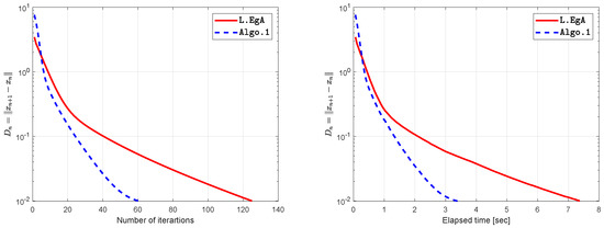
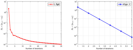
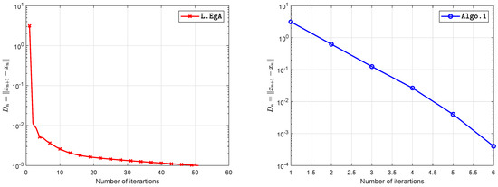
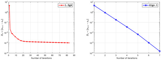
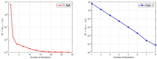
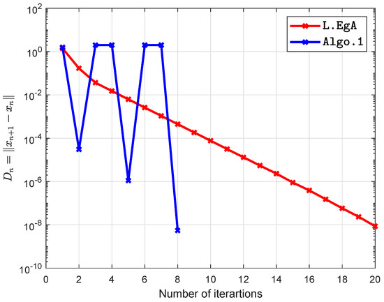
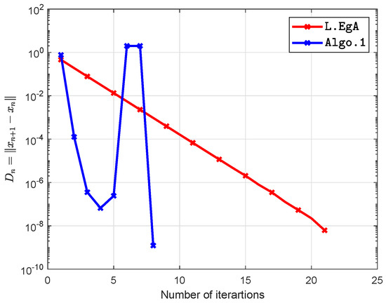
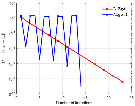
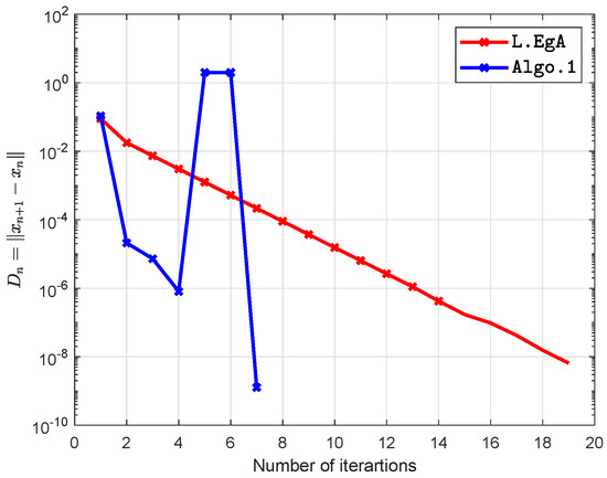
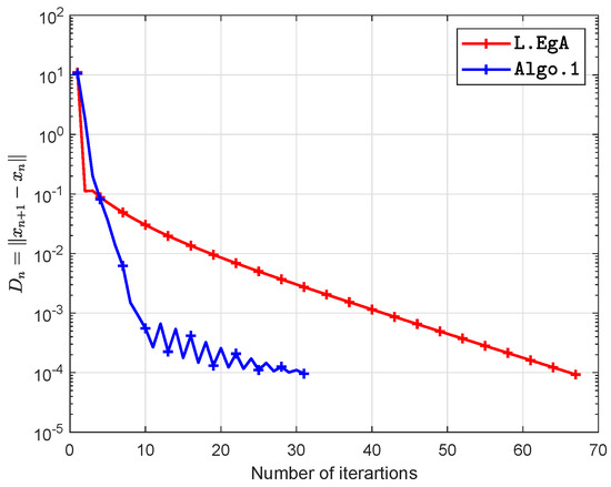
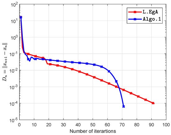
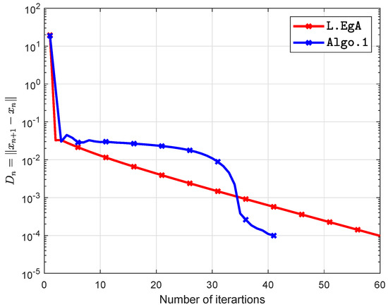
Numerical conclusions have shown in Figure 1, Figure 2, Figure 3 and Figure 4 and Table 3. For these numerical experiments we take $u_{-1}=v_{-1}=u_0=v_0={(48,48,30,27,18,24)}^T$ and $\lambda =0.01,$$\sigma =0.026,$$\mu =0.024,$${\wp }_n=0.20,$${\lambda }_0=0.1.$

Table 1. Parameters for cost bi-function.

Unit j	$\stackrel{\circ }{{\mathit{\alpha }}_{\mathit{j}}}$	$\stackrel{\circ }{{\mathit{\beta }}_{\mathit{j}}}$	$\stackrel{\circ }{{\mathit{\gamma }}_{\mathit{j}}}$	$\stackrel{•}{{\mathit{\alpha }}_{\mathit{j}}}$	$\stackrel{•}{{\mathit{\beta }}_{\mathit{j}}}$	$\stackrel{•}{{\mathit{\gamma }}_{\mathit{j}}}$
1	0.04	2	0	2	1	25
2	0.035	1.75	0	1.75	1	28.5714
3	0.125	1	0	1	1	8
4	0.0116	3.25	0	3.25	1	86.2069
5	0.05	3	0	3	1	20
6	0.05	3	0	3	1	20

Table 2. Values used for constraint set.

j	${\mathit{u}}_{\mathit{j}}^{\mathbf{min}}$	${\mathit{u}}_{\mathit{j}}^{\mathbf{max}}$
1	0	80
2	0	80
3	0	50
4	0	55
5	0	30
6	0	40

Figure 1. Example 1 while tolerance is $0.01.$

Figure 2. Example 1 while tolerance is $0.001.$

Figure 3. Example 1 while tolerance is $0.0001.$

Figure 4. Example 1 while tolerance is $0.00001.$

Table 3. Figure 1, Figure 2, Figure 3 and Figure 4 numerical values.

	L.EgA		Algo.1
TOL	Iter.	time (s)	Iter.	time (s)
0.01	125	7.3692	61	3.4055
$u_{\mathtt{L}.\mathtt{EgA}}^{*}=(47.3245,47.3245,47.3245,47.3245,47.3245,47.3245)$
$u_{\mathtt{Algo}.\mathtt{1}}^{*}=(47.3245,47.3245,47.3245,47.3245,47.3245,47.3245)$
0.001	2761	193.3939	2063	150.6757
$u_{\mathtt{L}.\mathtt{EgA}}^{*}=(47.3245,47.3245,47.3245,47.3245,47.3245,47.3245)$
$u_{\mathtt{Algo}.\mathtt{1}}^{*}=(47.3245,47.3245,47.3245,47.3245,47.3245,47.3245)$
0.0001	11,526	818.7184	4687	324.3571
$u_{\mathtt{L}.\mathtt{EgA}}^{*}=(47.3245,47.3245,47.3245,47.3245,47.3245,47.3245)$
$u_{\mathtt{Algo}.\mathtt{1}}^{*}=(47.3245,47.3245,47.3245,47.3245,47.3245,47.3245)$
0.00001	20,946	1449.3959	7307	526.9766
$u_{\mathtt{L}.\mathtt{EgA}}^{*}=(47.3245,47.3245,47.3245,47.3245,47.3245,47.3245)$
$u_{\mathtt{Algo}.\mathtt{1}}^{*}=(47.3245,47.3245,47.3245,47.3245,47.3245,47.3245)$

Example 2.

Assume that the following cost bifunction f defined by

$$f(u,v)=⟨(A{A}^T+B+C)u,v-u⟩,$$

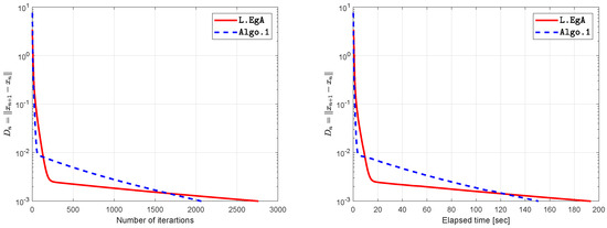
on the convex set $C=\{u\in {\mathbb{R}}^n:Du\le d\}$ while D is an $100\times n$ matrix and d is a non-negative vector. In the above bifunction definition we take A is an $n\times n$ matrix, B is an $n\times n$ skew-symmetric matrix, C is an $n\times n$ diagonal matrix having diagonal entries are non-negative. The matrices are generated as; A = rand(n), K = rand(n), $B=0.5K-0.5K^T$ and C = diag(rand(n,1)). The bifunction f is monotone and having Lipschitz-type constants are $c_1=c_2=\frac{1}{2}\parallel A{A}^T+B+C\parallel .$ Numerical results are presented in the Figure 5, Figure 6, Figure 7 and Figure 8 and Table 4. For these numerical experiments we take $u_{-1}=v_{-1}=u_0=v_0={(1,1,\cdots ,1)}^T$ and $\lambda =\frac{1}{10c_1},$$\sigma =\frac{1}{8c_1},$$\mu =\frac{1}{8.2c_1},$${\wp }_n=\frac{1}{5},$${\lambda }_0=1/4c_1.$

Figure 5. Example 2 for average number of iterations while $n=5.$

Figure 6. Example 2 for average number of iterations while $n=10.$

Figure 7. Example 2 for average number of iterations while $n=20.$

Figure 8. Example 2 for average number of iterations while $n=40.$

Table 4. Numerical results for Figure 5, Figure 6, Figure 7 and Figure 8.

	L.EgA			Algo.1
n	T. Samples	Avg Iter.	Avg time(s)	Avg Iter.	Avg time(s)
5	10	35	0.8066	6	0.1438
10	10	51	1.1779	6	0.1302
20	10	84	1.7441	7	0.1801
40	10	30	0.6859	8	0.1999

Example 3.

Assume that $F:{\mathbb{R}}^2\to {\mathbb{R}}^2$ is defined by

$$F\left(u\right)=\left(\begin{array}{c}0.5u_1{u}_2-2u_2-{10}^7\\ -4u_1-0.1u_2^2-{10}^7\end{array}\right)$$

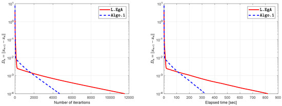
with $C=\{u\in {\mathbb{R}}^2:{(u_1-2)}^2+{(u_2-2)}^2\le 1\}.$ It is not hard to check that F is Lipschitz continuous with $L=5$ and pseudomonotone. The step size $\lambda ={10}^{-6}$ for Lyashko et al. [25] and ${\lambda }_0=0.1$, $\sigma =0.129,$${\wp }_n=0.20$ and $\mu =0.119.$ Computational results are shown in the Table 5 and in Figure 9, Figure 10, Figure 11 and Figure 12.

Table 5. Numerical results for Figure 9, Figure 10, Figure 11 and Figure 12.

	L.EgA		Algo.1
${\mathit{u}}_{\mathbf{0}}$	Iter.	time(s)	Iter.	time(s)
$(1.5,1.7)$	20	0.7506	8	0.5316
$(2.0,3.0)$	21	0.7879	8	0.6484
$(1.0,2.0)$	23	1.1450	14	0.9730
$(2.7,2.6)$	19	0.7254	7	0.5835

Figure 9. Example 3 while $u_0=(1.5,1.7).$

Figure 10. Example 3 while $u_0=(2,3).$

Figure 11. Example 3 while $u_0=(1,2).$

Figure 12. Example 3 while $u_0=(2.7,2.6).$

Example 4.

Let $F:{\mathbb{R}}^2\to {\mathbb{R}}^2$ is defined by

$$F\left(u\right)=\left(\begin{array}{c}(u_1^2+{(u_2-1)}^2)(1+u_2)\\ -u_1^3-u_1{(u_2-1)}^2\end{array}\right)$$

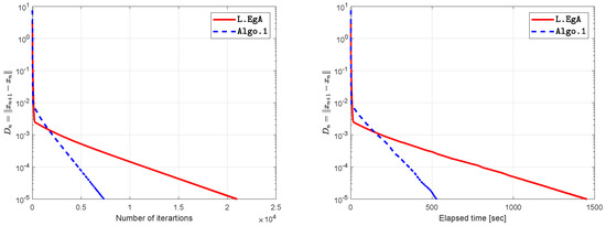
and $C=\{u\in {\mathbb{R}}^2:{(u_1-2)}^2+{(u_2-2)}^2\le 1\}.$ Here, F is not monotone but pseudomonotone on C and L-Lipschitz continuous through $L=5$ (see, e.g., [33]). The stepsize $\lambda ={10}^{-2}$ for Lyashko et al. [25] and ${\lambda }_0=0.01$, $\sigma =0.129$, ${\wp }_n=0.15$ and $\mu =0.119.$ The computational experimental findings are written in Table 6 and in Figure 13, Figure 14 and Figure 15.

Table 6. Figure 13, Figure 14 and Figure 15 numerical values.

	L.EgA		Algo.1
${\mathit{u}}_{\mathbf{0}}$	Iter.	time(s)	Iter.	time(s)
$(10,10)$	67	1.9151	31	1.0752
$(-10,-10)$	92	2.5721	71	2.0469
$(10,20)$	60	1.7689	41	1.1864

Figure 13. Example 4 while $u_0=(10,10).$

Figure 14. Example 4 while $u_0=(-10,-10).$

Figure 15. Example 4 while $u_0=(10,20).$

6. Conclusions

We have established an extragradient-like method to solve pseudomonotone equilibrium problems in real Hilbert space. The main advantage of the proposed method is that an iterative sequence has been incorporated with a certain step size evaluation formula. The step size formula is updated for each iteration based on the previous iterations. Numerical findings were presented to show our algorithm’s numerical efficiency compared with other methods. Such numerical investigations indicate that inertial effects often generally improve the effectiveness of the iterative sequence in this context.

References

- Blum, E. From optimization and variational inequalities to equilibrium problems. Math. Stud. 1994, 63, 123–145. [Google Scholar]
- Facchinei, F.; Pang, J.S. Finite-Dimensional Variational Inequalities and Complementarity Problems; Springer Science & Business Media: Berlin/Heidelberg, Germany, 2007. [Google Scholar]
- Konnov, I. Equilibrium Models and Variational Inequalities; Elsevier: Amsterdam, The Netherlands, 2007; Volume 210. [Google Scholar]
- Muu, L.D.; Oettli, W. Convergence of an adaptive penalty scheme for finding constrained equilibria. Nonlinear Anal. Theory Methods Appl. 1992, 18, 1159–1166. [Google Scholar]
- Combettes, P.L.; Hirstoaga, S.A. Equilibrium programming in Hilbert spaces. J. Nonlinear Convex Anal. 2005, 6, 117–136. [Google Scholar]
- Flåm, S.D.; Antipin, A.S. Equilibrium programming using proximal-like algorithms. Math. Program. 1996, 78, 29–41. [Google Scholar]
- Quoc, T.D.; Anh, P.N.; Muu, L.D. Dual extragradient algorithms extended to equilibrium problems. J. Glob. Optim. 2012, 52, 139–159. [Google Scholar]
- Quoc Tran, D.; Le Dung, M.; Nguyen, V.H. Extragradient algorithms extended to equilibrium problems. Optimization 2008, 57, 749–776. [Google Scholar]
- Santos, P.; Scheimberg, S. An inexact subgradient algorithm for equilibrium problems. Comput. Appl. Math. 2011, 30, 91–107. [Google Scholar]
- Takahashi, S.; Takahashi, W. Viscosity approximation methods for equilibrium problems and fixed point problems in Hilbert spaces. J. Math. Anal. Appl. 2007, 331, 506–515. [Google Scholar]
- Ur Rehman, H.; Kumam, P.; Kumam, W.; Shutaywi, M.; Jirakitpuwapat, W. The Inertial Sub-Gradient Extra-Gradient Method for a Class of Pseudo-Monotone Equilibrium Problems. Symmetry 2020, 12, 463. [Google Scholar] [CrossRef]
- Ur Rehman, H.; Kumam, P.; Argyros, I.K.; Alreshidi, N.A.; Kumam, W.; Jirakitpuwapat, W. A Self-Adaptive Extra-Gradient Methods for a Family of Pseudomonotone Equilibrium Programming with Application in Different Classes of Variational Inequality Problems. Symmetry 2020, 12, 523. [Google Scholar] [CrossRef]
- Ur Rehman, H.; Kumam, P.; Shutaywi, M.; Alreshidi, N.A.; Kumam, W. Inertial Optimization Based Two-Step Methods for Solving Equilibrium Problems with Applications in Variational Inequality Problems and Growth Control Equilibrium Models. Energies 2020, 13, 3293. [Google Scholar] [CrossRef]
- Hieu, D.V. New extragradient method for a class of equilibrium problems in Hilbert spaces. Appl. Anal. 2017, 97, 811–824. [Google Scholar] [CrossRef]
- Hammad, H.A.; ur Rehman, H.; De la Sen, M. Advanced Algorithms and Common Solutions to Variational Inequalities. Symmetry 2020, 12, 1198. [Google Scholar] [CrossRef]
- Ur Rehman, H.; Kumam, P.; Cho, Y.J.; Yordsorn, P. Weak convergence of explicit extragradient algorithms for solving equilibirum problems. J. Inequalities Appl. 2019, 2019. [Google Scholar] [CrossRef]
- Ur Rehman, H.; Kumam, P.; Abubakar, A.B.; Cho, Y.J. The extragradient algorithm with inertial effects extended to equilibrium problems. Comput. Appl. Math. 2020, 39. [Google Scholar] [CrossRef]
- Ur Rehman, H.; Kumam, P.; Argyros, I.K.; Deebani, W.; Kumam, W. Inertial Extra-Gradient Method for Solving a Family of Strongly Pseudomonotone Equilibrium Problems in Real Hilbert Spaces with Application in Variational Inequality Problem. Symmetry 2020, 12, 503. [Google Scholar] [CrossRef]
- Koskela, P.; Manojlović, V. Quasi-Nearly Subharmonic Functions and Quasiconformal Mappings. Potential Anal. 2012, 37, 187–196. [Google Scholar] [CrossRef]
- Ur Rehman, H.; Kumam, P.; Argyros, I.K.; Shutaywi, M.; Shah, Z. Optimization Based Methods for Solving the Equilibrium Problems with Applications in Variational Inequality Problems and Solution of Nash Equilibrium Models. Mathematics 2020, 8, 822. [Google Scholar] [CrossRef]
- Rehman, H.U.; Kumam, P.; Dong, Q.L.; Peng, Y.; Deebani, W. A new Popov’s subgradient extragradient method for two classes of equilibrium programming in a real Hilbert space. Optimization 2020, 1–36. [Google Scholar] [CrossRef]
- Yordsorn, P.; Kumam, P.; ur Rehman, H.; Ibrahim, A.H. A Weak Convergence Self-Adaptive Method for Solving Pseudomonotone Equilibrium Problems in a Real Hilbert Space. Mathematics 2020, 8, 1165. [Google Scholar] [CrossRef]
- Todorčević, V. Harmonic Quasiconformal Mappings and Hyperbolic Type Metrics; Springer International Publishing: Berlin/Heidelberg, Germany, 2019. [Google Scholar] [CrossRef]
- Yordsorn, P.; Kumam, P.; Rehman, H.U. Modified two-step extragradient method for solving the pseudomonotone equilibrium programming in a real Hilbert space. Carpathian J. Math. 2020, 36, 313–330. [Google Scholar]
- Lyashko, S.I.; Semenov, V.V. A new two-step proximal algorithm of solving the problem of equilibrium programming. In Optimization and Its Applications in Control and Data Sciences; Springer: Berlin/Heidelberg, Germany, 2016; pp. 315–325. [Google Scholar]
- Polyak, B.T. Some methods of speeding up the convergence of iteration methods. USSR Comput. Math. Math. Phys. 1964, 4, 1–17. [Google Scholar] [CrossRef]
- Bianchi, M.; Schaible, S. Generalized monotone bifunctions and equilibrium problems. J. Optim. Theory Appl. 1996, 90, 31–43. [Google Scholar] [CrossRef]
- Mastroeni, G. On Auxiliary Principle for Equilibrium Problems. In Nonconvex Optimization and Its Applications; Springer: New York, NY, USA, 2003; pp. 289–298. [Google Scholar] [CrossRef]
- Bauschke, H.H.; Combettes, P.L. Convex Analysis and Monotone Operator Theory in Hilbert Spaces; Springer: Berlin/Heidelberg, Germany, 2011; Volume 408. [Google Scholar]
- Tiel, J.V. Convex Analysis; John Wiley: Hoboken, NJ, USA, 1984. [Google Scholar]
- Alvarez, F.; Attouch, H. An inertial proximal method for maximal monotone operators via discretization of a nonlinear oscillator with damping. Set Valued Anal. 2001, 9, 3–11. [Google Scholar] [CrossRef]
- Opial, Z. Weak convergence of the sequence of successive approximations for nonexpansive mappings. Bull. Am. Math. Soc. 1967, 73, 591–597. [Google Scholar] [CrossRef]
- Shehu, Y.; Dong, Q.L.; Jiang, D. Single projection method for pseudo-monotone variational inequality in Hilbert spaces. Optimization 2019, 68, 385–409. [Google Scholar] [CrossRef]
Publisher’s Note: MDPI stays neutral with regard to jurisdictional claims in published maps and institutional affiliations. |
© 2020 by the authors. Licensee MDPI, Basel, Switzerland. This article is an open access article distributed under the terms and conditions of the Creative Commons Attribution (CC BY) license (http://creativecommons.org/licenses/by/4.0/).