Computational Study of Singularly Perturbed Neurodynamical Models via Cubic B-Spline

Abstract

This work focuses on solving the singularly perturbed generalized Hodgkin-Huxley (HH) problem. The HH equation is numerically solved by a collocation approach using third-degree splines. The forward difference technique is utilized for time discretization, while $\theta$-weighted schemes are employed for space discretization. Solving non-linear models using discretization and quasi-linearization results in a set of linear algebraic equations, which are solved using matrices. Furthermore, Von Neumann’s (VN) stability and Spectral Radius (S.R) reveal that the suggested technique is unconditionally stable. To assess the performance and accuracy of this method, absolute error (AE), $L_2$, and $L_{\infty }$ norms are offered. The results align with the literature. Simulation results show that the proposed strategy produces accurate results.

1. Introduction

Alan Hodgkin and Andrew Huxley’s investigation into the ionic currents that generate neuron action potentials is considered one of the most significant scientific breakthroughs of the 20th century. Not surprisingly, that case has attracted the attention of historians, neuroscientists, and philosophers of science. In 1963, the Nobel Prize in Physiology and Medicine was awarded to Hodgkin and Huxley for their remarkable achievements. They established the model using data from several tests on nerve conduction in the squid Loligo’s enormous axon. According to their description, the axon is a separate cable composed of a neural core encased in a membrane that permits currents to move back and forth through ion and capacitive transport mechanisms [1]. In 1952, a well-known nonlinear one-dimensional response diffusion system that approximated nerve conduction in the massive squid Logilo axon was devised. They came to the following systems:

$$\begin{array}{cc}\hfill & {\displaystyle \frac{\partial \mathrm{u}}{\partial \mathrm{t}}}-{\displaystyle \frac{{\partial }^2\mathrm{u}}{\partial {\zeta }^2}}=g_{N_a}{m}^{3}h({\mathrm{u}}_{N_a}-\mathrm{u})+g_k{n}^4({\mathrm{u}}_k-\mathrm{u})+g_L({\mathrm{u}}_L-\mathrm{u})\hfill \\ & {\displaystyle \frac{\partial \mathrm{m}}{\partial \mathrm{t}}}={\displaystyle \frac{({\mathrm{m}}_{\infty }\left(\mathrm{u}\right)-\mathrm{m})}{{\tau }_m\left(\mathrm{u}\right)}}\hfill \\ \hfill & {\displaystyle \frac{\partial \mathrm{h}}{\partial \mathrm{t}}}={\displaystyle \frac{({\mathrm{h}}_{\infty }\left(\mathrm{u}\right)-\mathrm{h})}{{\tau }_h\left(\mathrm{u}\right)}}\hfill \\ \hfill & {\displaystyle \frac{\partial \mathrm{n}}{\partial \mathrm{t}}}={\displaystyle \frac{({\mathrm{n}}_{\infty }\left(\mathrm{u}\right)-\mathrm{n})}{{\tau }_n\left(\mathrm{u}\right)}}\hfill \end{array}$$

(1)

where $\mathrm{t}$, the time, and $\zeta$, the length of the axon longitudinally, are the independent variables. The transmembrane potential $\mathrm{u}$ is the dependent variable, whereas the other variables $\mathrm{m}$, $\mathrm{h}$, and $\mathrm{n}$ stand for certain conductance. The axon membrane potential’s logical dynamics are denoted by Equation (1). Evans and Shenk [2] studied the system provided by Equation (1), and the following equation was presented:

$${\displaystyle \frac{\partial \mathrm{u}}{\partial \mathrm{t}}}-ϵ{\displaystyle \frac{{\partial }^2\mathrm{u}}{\partial {\zeta }^2}}=\varpi \mathrm{u}(1-{\mathrm{u}}^{\delta })({\mathrm{u}}^{\delta }-\gamma ),\zeta \in (a,b),\mathrm{t}\ge 0,$$

(2)

where $\varpi$ is a real number, $\delta =1,2,3,\dots ,\gamma \in (0,1)$ and $ϵ\ll 1$.

The conditions associated with the exact solutions are

$$\begin{array}{cc}\hfill & \mathrm{u}(\zeta ,0)={\left[{\displaystyle \frac{\gamma }{2}}+{\displaystyle \frac{\gamma }{2}}tanh\left(\varphi \gamma \left({\displaystyle \frac{\zeta }{\sqrt{ϵ}}}\right)\right)\right]}^{{\displaystyle \frac{1}{\delta }}},\zeta \in (a,b)\hfill \\ \hfill & \mathrm{u}(a,\mathrm{t})={\left[{\displaystyle \frac{\gamma }{2}}+{\displaystyle \frac{\gamma }{2}}tanh\left(\varphi \gamma \left({\displaystyle \frac{a}{\sqrt{ϵ}}}+{\displaystyle \frac{\left(1+\delta -\gamma \right)\rho \mathrm{t}}{2\left(1+\delta \right)}}\right)\right)\right]}^{{\displaystyle \frac{1}{\delta }}},\mathrm{t}\ge 0\hfill \\ \hfill & \mathrm{u}(b,\mathrm{t})={\left[{\displaystyle \frac{\gamma }{2}}+{\displaystyle \frac{\gamma }{2}}tanh\left(\varphi \gamma \left({\displaystyle \frac{b}{\sqrt{ϵ}}}+{\displaystyle \frac{\left(1+\delta -\gamma \right)\rho \mathrm{t}}{2\left(1+\delta \right)}}\right)\right)\right]}^{{\displaystyle \frac{1}{\delta }}},\mathrm{t}\ge 0\hfill \end{array}$$

(3)

The exact solution is given by

$$\mathrm{u}(\zeta ,\mathrm{t})={\left[{\displaystyle \frac{\gamma }{2}}+{\displaystyle \frac{\gamma }{2}}tanh\left(\varphi \gamma \left({\displaystyle \frac{\zeta }{\sqrt{ϵ}}}+{\displaystyle \frac{\left(1+\delta -\gamma \right)\rho \mathrm{t}}{2\left(1+\delta \right)}}\right)\right)\right]}^{{\displaystyle \frac{1}{\delta }}},$$

(4)

where $\varphi ={\displaystyle \frac{\delta \rho }{4(1+\delta )}}$ and $\rho =\sqrt{4\varpi (1+\delta )}$.

The solution of the generalized Huxley (GH) equation was suggested by Hashim et al. [3] using the Adomian decomposition method (ADM). Batiha et al. [4] employed the Variational iteration method (VIM) to simulate the GH equation. Sangwan et al. suggested a three-step Taylor Galerkin approach [5]. They examined how the HH equation behaved when $ϵ\to 0$. The boundary layer has been more sharply captured using the Shishkin mesh. The HH equation was solved by Aderogba and Chapwanya [6] using a positive and bounded nonstandard finite difference method (FDM). Macias-Díaz et al. [7] have presented a non-standard FDM to estimate the solution of an extended Burgers-Huxley (BH) equation. To solve the generalized BH equation, Sari et al. [8] combined a fourth-order Runge–Kutta approach with an up to tenth-order FDM. A uniform convergent technique with piecewise uniform mesh was introduced by Kaushik and Sharma [9] for the singularly perturbed unsteady generalized BH problem. This scheme combines the FDM and the Euler implicit method. Numerous other numerical methods, like VIM [10], the Galerkin method [11], etc., are developed to solve the HH equation.

Several numerical methods, such as finite difference methods, finite element methods, and collocation-based schemes, have recently been proposed to solve singularly perturbed differential equations arising in neurodynamical and biological models. Many of these techniques have drawbacks, such as decreased stability in the presence of boundary layers, higher processing costs, or loss of smoothness in the numerical solution, even if they have shown respectable accuracy [12,13,14].

To overcome these difficulties, the current study uses a cubic B-spline collocation method (CBSCM). Compared with current methods, the proposed strategy has several advantages. First, higher-order continuity is offered by cubic B-splines, which is especially advantageous for neurodynamical models where smooth solution profiles have physical significance. Second, compared to global polynomial-based techniques, the local support property of B-spline basis functions results in sparse and well-conditioned algebraic systems, improving computational efficiency. Additionally, without the need for extremely fine meshes or unique layer-adapted grids, the technique successfully captures sharp boundary layers caused by minor perturbation factors [12,14,15]. B-spline is used in various fields, especially in finding approximate solutions. A regularized CBSCM for calculating the impact force time history is shown in a study in [16], mitigating the limitations of the well-posed problem. The cubic B-spline (CBS) function, which controls collocation point mesh size, follows a typical impact event profile. The numerical solution of the non-linear Foam-Drainage model (FDM) was estimated using the collocation approach in connection with the CBS basis [17,18]. The B-spline collocation method (BSCM) is also utilized for the solution of incompressible Navier–Stokes equations [19]. Akbar et al. use the quintic BSCM to find the solution of third-order equations, utilizing finite difference and theta-weighted schemes [20]. A fourth-order BSCM was used for the numerical investigation of the Burgers-Fisher problem [21]. Dag and Saka investigated the numerical solution of an equal-width equation using CBSCM [22]. The modified quintic B-spline approach is used to solve Burgers’ equations and the convection-diffusion equation [23]. Dhiman et al. present an implicit collocation algorithm for Caputo time-fractional PDE, utilizing extended CBS functions to discretize derivatives for the space variable [24]. A trigonometric and exponential CBS technique for the evaluation of the time-fractional diffusion equation is also reported [25,26].

The remaining paper is organized in the following manner. The CBS is defined in the Section 2. Then, in Section 3, we discuss the numerical scheme. In Section 4, the stability analysis is covered. Section 5 will give numerical experiments for various test problems. In the, Section 6 we conclude our article.

2. Formulation of Third Degree B-Spline

In this section, the introduction of CBS is discussed. The region $\left[a,b\right]$ is divided into uniform-sized finite elements of length h by the knots ${\zeta }_m$ such that $a={\zeta }_0<{\zeta }_1<{\zeta }_2<···<{\zeta }_m=b$. Where $h=(b-a)/N$ and a and b are the lower and upper limits. The set of splines $\left\{B_0,B_1,\dots ,B_N,B_{N+1}\right\}$ forms a basis for functions defined over $\left[a,b\right]$. Thus, an approximation solution $u_N(\zeta ,t)$ can be expressed in terms of the CBS functions as

$$u_N(\zeta ,t)=\sum _{m=-1}^{N+1}{C}_m\left(t\right)B_m\left(\zeta \right),$$

(5)

where $C\left(t\right)$ are the time-dependent quantities that need to be evaluated and $B_m\left(\zeta \right)$ are CBS functions.

The CBS basis function for $i=-1,\dots ,N+1$, is defined as

$$B_m\left(\zeta \right)={\displaystyle \frac{1}{6h^3}}\left\{\begin{array}{cc}{\left(\zeta -{\zeta }_{m-2}\right)}^3,\hfill & \left[{\zeta }_{m-2},{\zeta }_{m-1}\right)\hfill \\ -3{\left(\zeta -{\zeta }_{m-1}\right)}^3+3h{\left(\zeta -{\zeta }_{m-1}\right)}^2+3h^2\left(\zeta -{\zeta }_{m-1}\right)+h^3,\hfill & \left[{\zeta }_{m-1},{\zeta }_m\right)\hfill \\ -3{\left({\zeta }_{m+1}-\zeta \right)}^3+3h{\left({\zeta }_{m+1}-\zeta \right)}^2+3h^2\left({\zeta }_{m+1}-\zeta \right)+h^3,\hfill & \left[{\zeta }_m,{\zeta }_{m+1}\right)\hfill \\ {\left({\zeta }_{m+2}-\zeta \right)}^3,\hfill & \left[{\zeta }_{m+1},{\zeta }_{m+2}\right)\hfill \\ 0,\hfill & \mathrm{otherwise}.\hfill \end{array}\right.$$

(6)

Using approximate Function (5) and CBS (6), the values of B-spline at different $\zeta$ are displayed in Table 1. The values of $u\left(\zeta \right)$, $u^{\prime }\left(\zeta \right)$, and $u^{″}\left(\zeta \right)$ at the knots are determined in terms of $C_m$ by

$$\begin{array}{cc}\hfill u_m\left(\zeta \right)& ={\displaystyle \frac{1}{6}}(C_{m-1}+4C_m+C_{m+1}),\hfill \\ \hfill u_m^{\prime }\left(\zeta \right)& ={\displaystyle \frac{1}{2h}}(C_{m+1}-C_{m-1}),\hfill \\ \hfill u_m^{″}\left(\zeta \right)& ={\displaystyle \frac{1}{h^2}}(C_{m-1}-2C_m+C_{m+1}),\hfill \end{array}$$

(7)

where $u_m^{\prime }\left(\zeta \right)$ and $u_m^{″}\left(\zeta \right)$ denote the first and second differentiation, respectively, concerning $\zeta$.

Table 1. $B_i\left(\zeta \right)$ and its derivatives at nodal points.

	${\mathit{\zeta }}_{\mathit{i}-2}$	${\mathit{\zeta }}_{\mathit{i}-1}$	${\mathit{\zeta }}_{\mathit{i}}$	${\mathit{\zeta }}_{\mathit{i}+1}$	${\mathit{\zeta }}_{\mathit{i}+2}$
$B_i\left(\zeta \right)$	0	1	4	1	0
$B_i^{\prime }\left(\zeta \right)$	0	${\displaystyle \frac{-3}{h}}$	0	${\displaystyle \frac{3}{h}}$	0
$B_i^{″}\left(\zeta \right)$	0	${\displaystyle \frac{6}{h^2}}$	${\displaystyle \frac{-12}{h^2}}$	${\displaystyle \frac{6}{h^2}}$	0

3. Numerical Scheme

Consider the generalized HH equation,

$${\mathrm{u}}_{\mathrm{t}}-ϵ{\mathrm{u}}_{\zeta \zeta }=\varpi \mathrm{u}(1-{\mathrm{u}}^{\delta })({\mathrm{u}}^{\delta }-\gamma ),$$

(8)

After rearranging

$${\mathrm{u}}_{\mathrm{t}}-ϵ{\mathrm{u}}_{\zeta \zeta }-\varpi \left(\left(1+\gamma \right){\mathrm{u}}^{\delta +1}-{\mathrm{u}}^{2\delta +1}-\gamma \mathrm{u}\right)=0,$$

(9)

The time derivative has been approximated by the finite difference formula, and using the $\theta$-weighted scheme for space discretization, Equation (9) takes the following form:

$$\begin{array}{cc}\hfill & {\displaystyle \frac{{\mathrm{u}}^{n+1}-{\mathrm{u}}^n}{d\mathrm{t}}}+\theta \left(-ϵ{\mathrm{u}}_{\zeta \zeta }^{n+1}-\varpi \left(\left(1+\gamma \right){\left({\mathrm{u}}^{\delta +1}\right)}^{n+1}-{\left({\mathrm{u}}^{2\delta +1}\right)}^{n+1}-\gamma {\mathrm{u}}^{n+1}\right)\right)\hfill \\ & =-\left(1-\theta \right)\left(-ϵ{\mathrm{u}}_{\zeta \zeta }^n-\varpi \left(\left(1+\gamma \right){\left({\mathrm{u}}^{\delta +1}\right)}^n-{\left({\mathrm{u}}^{2\delta +1}\right)}^n-\gamma {\mathrm{u}}^n\right)\right),\hfill \end{array}$$

(10)

Using quasi linearization described below, the non-linear terms ${\left({\mathrm{u}}^{\delta +1}\right)}^{n+1}$ and ${\left({\mathrm{u}}^{2\delta +1}\right)}^{n+1}$ are linearized.

$$\begin{array}{cc}\hfill & {\left({\mathrm{u}}^{\delta +1}\right)}^{n+1}={\left({\mathrm{u}}^{\delta +1}\right)}^n+\left(\delta +1\right){\left({\mathrm{u}}^{\delta }\right)}^n\left({\mathrm{u}}^{n+1}-{\mathrm{u}}^n\right),\hfill \\ \hfill & {\left({\mathrm{u}}^{2\delta +1}\right)}^{n+1}={\left({\mathrm{u}}^{2\delta +1}\right)}^n+\left(2\delta +1\right){\left({\mathrm{u}}^{2\delta }\right)}^n\left({\mathrm{u}}^{n+1}-{\mathrm{u}}^n\right).\hfill \end{array}$$

(11)

Substituting Equation (11) into Equation (10), which gives

$$\begin{array}{cc}\hfill & \left(1-\theta d\mathrm{t}\varpi \left(1+\gamma \right)\left(\delta +1\right){\left({\mathrm{u}}^{\delta }\right)}^n-\theta d\mathrm{t}\varpi \left(2\delta +1\right){\left({\mathrm{u}}^{2\delta }\right)}^n-\gamma \right){\mathrm{u}}^{n+1}\hfill \\ & -\left(\theta d\mathrm{t}ϵ\right){\mathrm{u}}_{\zeta \zeta }^{n+1}={\mathrm{u}}^n-\varpi \theta d\mathrm{t}\left(\delta \left(1+\gamma \right){\left({\mathrm{u}}^{\delta +1}\right)}^n-2\delta {\left({\mathrm{u}}^{2\delta +1}\right)}^n\right)\hfill \\ & -\left(1-\theta \right)d\mathrm{t}\left(-ϵ{\mathrm{u}}_{\zeta \zeta }^n-\varpi \left(\left(1+\gamma \right){\left({\mathrm{u}}^{\delta +1}\right)}^n-{\left({\mathrm{u}}^{2\delta +1}\right)}^n-\gamma {\mathrm{u}}^n\right)\right).\hfill \end{array}$$

(12)

Subsequently, the approximate solution, 1st and 2nd derivatives are obtained using the CBS as follows:

$$\begin{array}{cc}\hfill & \mathrm{u}(\zeta ,\mathrm{t})=\sum _{i=-1}^{N+1}{\mathrm{C}}_i\left(\mathrm{t}\right){\mathrm{B}}_i\left(\zeta \right),\hfill \\ \hfill & {\mathrm{u}}_{\zeta }(\zeta ,\mathrm{t})=\sum _{i=-1}^{N+1}{\mathrm{C}}_i\left(\mathrm{t}\right){\mathrm{B}}_i^{\prime }\left(\zeta \right),\hfill \\ \hfill & {\mathrm{u}}_{\zeta \zeta }(\zeta ,\mathrm{t})=\sum _{i=-1}^{N+1}{\mathrm{C}}_i\left(\mathrm{t}\right){\mathrm{B}}_i^{″}\left(\zeta \right).\hfill \end{array}$$

(13)

Substituting Equation (13) into Equation (12) with $\zeta ={\zeta }_j$ yields the following system:

$$\begin{array}{cc}\hfill & \left(1-\theta d\mathrm{t}\varpi \left(1+\gamma \right)\left(\delta +1\right){\left({\mathrm{u}}^{\delta }\right)}^n-\theta d\mathrm{t}\varpi \left(2\delta +1\right){\left({\mathrm{u}}^{2\delta }\right)}^n-\gamma \right)\hfill \\ & \sum _{i=-1}^{N+1}{\mathrm{C}}_i^{n+1}{\mathrm{B}}_i\left({\zeta }_{\mathrm{j}}\right)-\left(\theta d\mathrm{t}ϵ\right)\sum _{i=-1}^{N+1}{\mathrm{C}}_i^{n+1}{\mathrm{B}}_i^{″}\left({\zeta }_{\mathrm{j}}\right)=\sum _{i=-1}^{N+1}{\mathrm{C}}_i^n\left(\mathrm{t}\right){\mathrm{B}}_i\left({\zeta }_{\mathrm{j}}\right)\hfill \\ & -\varpi \theta d\mathrm{t}\left(\delta \left(1+\gamma \right){\left({\mathrm{u}}^{\delta }\right)}^n-2\delta {\left({\mathrm{u}}^{2\delta }\right)}^n\right)\sum _{i=-1}^{N+1}{\mathrm{C}}_i^n{\mathrm{B}}_i\left({\zeta }_{\mathrm{j}}\right)-\left(1-\theta \right)d\mathrm{t}\hfill \\ & \left(-ϵ\sum _{i=-1}^{N+1}{\mathrm{C}}_i^n{\mathrm{B}}_i^{″}\left({\zeta }_{\mathrm{j}}\right)-\varpi \left(\left(1+\gamma \right){\left({\mathrm{u}}^{\delta }\right)}^n-{\left({\mathrm{u}}^{2\delta }\right)}^n-\gamma \right)\sum _{i=-1}^{N+1}{\mathrm{C}}_i^n{\mathrm{B}}_i\left({\zeta }_{\mathrm{j}}\right)\right).\hfill \end{array}j=1,\dots ,N+1$$

(14)

After rearranging

$$\begin{array}{cc}\hfill & \left(1-\theta d\mathrm{t}\varpi \left(1+\gamma \right)\left(\delta +1\right){\left({\mathrm{u}}^{\delta }\right)}^n-\theta d\mathrm{t}\varpi \left(2\delta +1\right){\left({\mathrm{u}}^{2\delta }\right)}^n-\gamma \right)\hfill \\ \hfill & \sum _{i=-1}^{N+1}{\mathrm{C}}_i^{n+1}{\mathrm{B}}_i\left({\zeta }_{\mathrm{j}}\right)-\left(\theta d\mathrm{t}ϵ\right)\sum _{i=-1}^{N+1}{\mathrm{C}}_i^{n+1}{\mathrm{B}}_i^{″}\left({\zeta }_{\mathrm{j}}\right)=\left[1-\varpi \theta d\mathrm{t}\left(\delta \left(1+\gamma \right){\left({\mathrm{u}}^{\delta }\right)}^n-2\delta {\left({\mathrm{u}}^{2\delta }\right)}^n\right)\right.\hfill \\ \hfill & \left.+\left(1-\theta \right)d\mathrm{t}\varpi \left(\left(1+\gamma \right){\left({\mathrm{u}}^{\delta }\right)}^n-{\left({\mathrm{u}}^{2\delta }\right)}^n-\gamma \right)\right]\sum _{i=-1}^{N+1}{\mathrm{C}}_i^n{\mathrm{B}}_i\left({\zeta }_{\mathrm{j}}\right)+\left(1-\theta \right)d\mathrm{t}ϵ\sum _{i=-1}^{N+1}{\mathrm{C}}_i^n{\mathrm{B}}_i^{″}\left({\zeta }_{\mathrm{j}}\right)\hfill \end{array}$$

(15)

The above system represents $N+1$ equations in $N+3$ unknowns ${\mathrm{C}}^{n+1}=({\mathrm{C}}_{-1}^{n+1}$, ${\mathrm{C}}_0^{n+1},\dots ,{\mathrm{C}}_{N+1}^{n+1})$. Two more equations are required to complete the system. For this purpose, boundary conditions are as follows:

$$\begin{array}{cc}\hfill & {\displaystyle \frac{1}{6}}(C_{-1}+4C_0+C_1)={\alpha }_1\left(\mathrm{t}\right),\hfill \\ \hfill & {\displaystyle \frac{1}{6}}(C_{N-1}+4C_N+C_{N+1})={\alpha }_2\left(\mathrm{t}\right).\hfill \end{array}$$

(16)

For finding a solution $\mathrm{u}(\zeta ,\mathrm{t})$, for simplicity we write $\mathrm{u}$ by utilizing CBS

$$\begin{array}{cc}\hfill & \mathrm{u}\left(\zeta ,\mathrm{t}\right)={\displaystyle \frac{1}{6}}\left({\mathrm{C}}_{i-1}+4{\mathrm{C}}_i+{\mathrm{C}}_{i+1}\right).\hfill \\ \hfill & {\mathrm{u}}_{\zeta }(\zeta ,\mathrm{t})={\displaystyle \frac{1}{2h}}\left(-{\mathrm{C}}_{i-1}+{\mathrm{C}}_{i+1}\right).\hfill \\ \hfill & {\mathrm{u}}_{\zeta \zeta }(\zeta ,\mathrm{t})={\displaystyle \frac{1}{h^2}}\left({\mathrm{C}}_{i-1}-2{\mathrm{C}}_i+{\mathrm{C}}_{i+1}\right).\hfill \end{array}$$

(17)

$$\begin{array}{cc}\hfill & \left({\displaystyle \frac{1}{6}}{P}_1+{\displaystyle \frac{1}{h^2}}{P}_2\right){\mathrm{C}}_{i-1}+\left(4P_1-{\displaystyle \frac{2}{h^2}}{P}_2\right){\mathrm{C}}_i+\left(P_1+{\displaystyle \frac{1}{h^2}}{P}_2\right){\mathrm{C}}_{i+1}=\hfill \\ \hfill & \left({\displaystyle \frac{1}{6}}{P}_3+{\displaystyle \frac{1}{h^2}}{P}_4\right){\mathrm{C}}_{i-1}+\left(4P_3-{\displaystyle \frac{2}{h^2}}{P}_4\right){\mathrm{C}}_i+\left(P_3+{\displaystyle \frac{1}{h^2}}{P}_4\right){\mathrm{C}}_{i+1}\hfill \end{array}$$

(18)

The above equation can also be written as

$$\begin{array}{cc}\hfill & Q_1{\mathrm{C}}_{i-1}+Q_2{\mathrm{C}}_i+Q_3{\mathrm{C}}_{i+1}=Q_4{\mathrm{C}}_{i-1}+Q_5{\mathrm{C}}_i+Q_6{\mathrm{C}}_{i+1}\hfill \end{array}$$

(19)

where

$$\begin{array}{cc}\hfill & Q_1={\displaystyle \frac{1}{6}}{P}_1+{\displaystyle \frac{1}{h^2}}{P}_2,Q_2=4P_1-{\displaystyle \frac{2}{h^2}}{P}_2,\hfill \\ & Q_3=P_1+{\displaystyle \frac{1}{h^2}}{P}_2,Q_4={\displaystyle \frac{1}{6}}{P}_3+{\displaystyle \frac{1}{h^2}}{P}_4\hfill \\ & Q_5=4P_3-{\displaystyle \frac{2}{h^2}}{P}_4,Q_6=P_3+{\displaystyle \frac{1}{h^2}}{P}_4\hfill \end{array}$$

(20)

and

$$\begin{array}{cc}\hfill & P_1=1-\theta d\mathrm{t}\varpi \left(1+\gamma \right)\left(\delta +1\right){\left({\mathrm{u}}^{\delta }\right)}^n-\theta d\mathrm{t}\varpi \left(2\delta +1\right){\left({\mathrm{u}}^{2\delta }\right)}^n-\gamma ,P_2=-\theta d\mathrm{t}ϵ,\hfill \\ & P_3=1-\varpi \theta d\mathrm{t}\left(\delta \left(1+\gamma \right){\left({\mathrm{u}}^{\delta }\right)}^n-2\delta {\left({\mathrm{u}}^{2\delta }\right)}^n\right)\hfill \\ & +\left(1-\theta \right)d\mathrm{t}\varpi \left(\left(1+\gamma \right){\left({\mathrm{u}}^{\delta }\right)}^n-{\left({\mathrm{u}}^{2\delta }\right)}^n-\gamma \right),\hfill \\ & P_4=\left(1-\theta \right)d\mathrm{t}ϵ\hfill \end{array}$$

(21)

In compact form the system can be written as

$${\mathrm{Z}}_1{\mathrm{C}}^{n+1}={\mathrm{Z}}_2{\mathrm{C}}^n,$$

(22)

where ${\mathrm{C}}^{n+1}$ represents the column matrix having dimensions $(N+3)\times 1$, and the coefficient matrices are the square matrices with dimensions $(N+3)\times (N+3)$.

Where

$$Z_1=\left[\begin{array}{ccccccc}0& 0& 0& 0& 0& \cdots & 0\\ Q_1\left({\zeta }_0\right)& Q_2\left({\zeta }_0\right)& Q_3\left({\zeta }_0\right)& 0& 0& \cdots & 0\\ 0& Q_1\left({\zeta }_1\right)& Q_2\left({\zeta }_1\right)& Q_3\left({\zeta }_1\right)& 0& \cdots & 0\\ ⋮& & \ddots & \ddots & \ddots & & ⋮\\ & & & Q_1\left({\zeta }_{m-1}\right)& Q_2\left({\zeta }_{m-1}\right)& Q_3\left({\zeta }_{m-1}\right)& 0\\ 0& \cdots & & 0& Q_1\left({\zeta }_m\right)& Q_2\left({\zeta }_m\right)& Q_3\left({\zeta }_m\right)\\ 0& \cdots & & 0& 0& 0& 0\end{array}\right]$$

$$Z_2=\left[\begin{array}{ccccccc}0& 0& 0& 0& 0& \cdots & 0\\ Q_4\left({\zeta }_0\right)& Q_5\left({\zeta }_0\right)& Q_6\left({\zeta }_0\right)& 0& 0& \cdots & 0\\ 0& Q_4\left({\zeta }_1\right)& Q_5\left({\zeta }_1\right)& Q_6\left({\zeta }_1\right)& 0& \cdots & 0\\ ⋮& & \ddots & \ddots & \ddots & & ⋮\\ & & & Q_4\left({\zeta }_{m-1}\right)& Q_5\left({\zeta }_{m-1}\right)& Q_6\left({\zeta }_{m-1}\right)& 0\\ 0& \cdots & & 0& Q_4\left({\zeta }_m\right)& Q_5\left({\zeta }_m\right)& Q_6\left({\zeta }_m\right)\\ 0& \cdots & & 0& 0& 0& 0\end{array}\right]$$

The first and the last rows of $Z_1$ and $Z_2$ can be replced by utilizing the boundary conditions using the definition CBS, defined in Equation (16).

To initialize the process, we use the initial condition; in this case, the system reduces to

$${\mathrm{I}}_1{\mathrm{C}}^0={\mathrm{I}}_2,$$

(23)

where

$${\mathrm{I}}_1=\left[\begin{array}{cccccc}{\displaystyle \frac{-3}{h}}& 0& {\displaystyle \frac{3}{h}}& \cdots & \cdots & 0\\ 1& 4& 1& & & ⋮\\ 0& 1& 4& 1& & ⋮\\ ⋮& & \ddots & \ddots & \ddots & ⋮\\ ⋮& & 1& 4& 1& ⋮\\ ⋮& & & 1& 4& 1\\ 0& \cdots & \cdots & {\displaystyle \frac{-3}{h}}& 0& {\displaystyle \frac{3}{h}}\end{array}\right],{\mathrm{C}}^0=\left[\begin{array}{c}{\mathrm{C}}_{-1}\\ {\mathrm{C}}_0\\ {\mathrm{C}}_1\\ ⋮\\ {\mathrm{C}}_{N-1}\\ {\mathrm{C}}_N\\ {\mathrm{C}}_{N+1}\end{array}\right],{\mathrm{I}}_2=\left[\begin{array}{c}{\mathrm{f}}^{\prime }\left({\zeta }_0\right)\\ \mathrm{f}\left({\zeta }_0\right)\\ \mathrm{f}\left({\zeta }_1\right)\\ ⋮\\ \mathrm{f}\left({\zeta }_{N-1}\right)\\ \mathrm{f}\left({\zeta }_N\right)\\ {\mathrm{f}}^{\prime }\left({\zeta }_N\right)\end{array}\right].$$

(24)

The system provided in Equation (22) can be used to obtain the unknown constant. Equation (5) can be used to estimate the numerical solution once these constants have been obtained.

4. Stability Analysis

The stability of the proposed approach is evaluated using VN stability analysis. To linearize the nonlinear terms, take ${\lambda }_1=max\left({\mathrm{u}}^{\delta }\right)$ and ${\lambda }_2=max\left({\mathrm{u}}^{2\delta }\right)$ as the local constants. Further, applying the Crank–Nicolson scheme, as follows:

$${\displaystyle \frac{{\mathrm{u}}^{n+1}-{\mathrm{u}}^n}{\delta \mathrm{t}}}-{\displaystyle \frac{ϵ}{2}}\left[{\mathrm{u}}_{\zeta \zeta }^{n+1}+{\mathrm{u}}_{\zeta \zeta }^n\right]={\displaystyle \frac{\varpi }{2}}\left[\left(1+\gamma \right){\lambda }_1\left({\mathrm{u}}^{n+1}+{\mathrm{u}}^n\right)-{\lambda }_2\left({\mathrm{u}}^{n+1}+{\mathrm{u}}^n\right)-\gamma \left({\mathrm{u}}^{n+1}+{\mathrm{u}}^n\right)\right],$$

(25)

Rearranging of terms gives

$${\displaystyle \frac{{\mathrm{u}}^{n+1}}{\delta \mathrm{t}}}-{\displaystyle \frac{ϵ}{2}}{\mathrm{u}}_{\zeta \zeta }^{n+1}-{\displaystyle \frac{\varpi }{2}}{\mathrm{u}}^{n+1}\left({\lambda }_1\left(1+\gamma \right)-{\lambda }_2-\gamma \right)={\displaystyle \frac{{\mathrm{u}}^n}{\delta \mathrm{t}}}-{\displaystyle \frac{ϵ}{2}}{\mathrm{u}}_{\zeta \zeta }^n-{\displaystyle \frac{\varpi }{2}}{\mathrm{u}}^n\left({\lambda }_1\left(1+\gamma \right)-{\lambda }_2-\gamma \right),$$

(26)

After using the CBS and taking $P_1=\left({\lambda }_1\left(1+\gamma \right)-{\lambda }_2-\gamma \right)$ we get

$$a_1{\mathrm{C}}_{i-1}^{n+1}+a_2{\mathrm{C}}_i^{n+1}+a_1{\mathrm{C}}_{i+1}^{n+1}=a_3{\mathrm{C}}_{i-1}^n+a_4{\mathrm{C}}_i^n+a_3{C}_{i+1}^n,$$

(27)

where

$$\begin{array}{cc}\hfill & a_1=\left(1-{\displaystyle \frac{3}{h^2}}ϵ\delta \mathrm{t}-{\displaystyle \frac{\varpi }{2}}{P}_1\delta \mathrm{t}\right),a_2=\left(4+{\displaystyle \frac{6}{h^2}}ϵ\delta \mathrm{t}-2\varpi P_1\delta \mathrm{t}\right),\hfill \\ \hfill & a_3=\left(1+{\displaystyle \frac{3}{h^2}}ϵ\delta \mathrm{t}+{\displaystyle \frac{\varpi }{2}}{P}_1\delta \mathrm{t}\right),a_4=\left(4-{\displaystyle \frac{6}{h^2}}ϵ\delta \mathrm{t}+2\varpi P_1\delta \mathrm{t}\right).\hfill \end{array}$$

(28)

Substituting the following into Equation (27)

$${\mathrm{C}}^n=e^{ijkh}{\delta }^n$$

(29)

The amplification factor is $\delta$, and k and h are the mode number and element size, respectively. By putting Equation (28) into Equation (27) and after further simplification we get

$${\displaystyle \frac{{\delta }^{n+1}}{{\delta }^n}}={\displaystyle \frac{B}{A}}$$

(30)

where

$$\begin{array}{c}\hfill \begin{array}{cc}\hfill & A=\left(2-{\displaystyle \frac{6}{h^2}}ϵ\delta \mathrm{t}-\varpi P_1\delta \mathrm{t}\right)cos\left(kh\right)+\left(4+{\displaystyle \frac{6}{h^2}}ϵ\delta \mathrm{t}-2\varpi P_1\delta \mathrm{t}\right),\hfill \\ \hfill & B=\left(2+{\displaystyle \frac{6}{h^2}}ϵ\delta \mathrm{t}+\varpi P_1\delta \mathrm{t}\right)cos\left(kh\right)+\left(4-{\displaystyle \frac{6}{h^2}}ϵ\delta \mathrm{t}+2\varpi P_1\delta \mathrm{t}\right).\hfill \end{array}\end{array}$$

(31)

Taking the modulus of Equation (30) gives $\left|\delta \right|\le 1$, Consequently, the approach is unconditionally stable.

5. Examples and Discussion

In order to verify the accuracy as well as efficiency of the approach, we examine numerical examples of generalized HH in this section. Here, $u_E$ and $u_A$ denote the exact and the proposed solutions, respectively. The calculation was performed using the following error norms:

• Maximum error norm:

  $$L_{\infty }=ma{x}_i|{\mathrm{u}}_E({\mathrm{x}}_{\mathrm{i}},{\mathrm{t}}_{\mathrm{i}})-{\mathrm{u}}_A({\mathrm{x}}_{\mathrm{i}},{\mathrm{t}}_{\mathrm{i}})|,$$
• $L_2$ error norm:

  $$L_2=\sqrt{h\sum _{i=1}^N{({\mathrm{u}}_E({\mathrm{x}}_{\mathrm{i}},{\mathrm{t}}_{\mathrm{i}})-{\mathrm{u}}_A({\mathrm{x}}_{\mathrm{i}},{\mathrm{t}}_{\mathrm{i}}))}^2},$$
• AE:

  $$AE=|{\mathrm{u}}_E({\mathrm{x}}_{\mathrm{i}},{\mathrm{t}}_{\mathrm{i}})-{\mathrm{u}}_A({\mathrm{x}}_{\mathrm{i}},{\mathrm{t}}_{\mathrm{i}})|,$$

The Rate of Convergence (ROC) is determined by

$$ROC={\displaystyle \frac{L_{\infty }\left(\delta t_i\right)}{L_{\infty }\left(\delta t_{i+1}\right)}}$$

(32)

The (S.R) is also provided, and the ROC in time is calculated using the formula above. The Haier Core m³ 7th Gen Y11-C system is utilized for the computational tasks, and MATLAB (R2020a) software is employed to complete them.

5.1. Example 1

Consider Equations (2)–(4) with various values of $\delta$. Here, $\gamma =0.001$, $ϵ=1$, and $\varpi =1$. The numerical solution obtained by CBS is compared with the exact solution and the solution obtained from ADM [3], VIM [10], and FDM [8]. The results of the proposed technique are better than the VIM and ADM but comparable with the FDM. At some points their results are slightly better, and at some points our results are good. In Table 2, a comparison of AE for the case $\delta =1$ is shown. Spatial and temporal step sizes are $h=0.1$ and $d\mathrm{t}=0.01$, respectively. Similarly, for the case $\delta =2$ and $\delta =3$ comparison of AE is shown in Table 3 and Table 4, respectively. Figure 1 shows the surface profile of AE at different values of $\delta =1,2,3$, which shows the agreement with [3]. Table 5 mentions $L_2$, $L_{\infty }$ error norms along the ROC and (S.R). The ROC shows that it converges linearly and the (S.R) is less than one and confirms that the given method is stable. Furthermore, by increasing the value of $\delta$, it is found that the accuracy of the CBS decreases.

Table 2. Comparison of AE for $\varpi =1$, $\gamma =0.001$, $ϵ=1$, and $\delta =1$ of Example 1.

$\mathit{\zeta }$	t	Exact	Approximate	AE	ADM [3]	VIM [10]	FDM [8]
0.1	0.05	5.0003E-04	5.0008E-04	5.2129E-08	2.4988E-08	2.4987E-08	1.0303E-08
	0.1	5.0004E-04	5.0009E-04	5.4500E-08	4.9975E-08	2.4987E-08	1.5063E-08
	1	5.0027E-04	5.0025E-04	1.8753E-08	4.9975E-07	2.4988E-08	2.2488E-08
0.5	0.05	5.0010E-04	5.0010E-04	1.8820E-09	2.4988E-08	4.9975E-08	2.3138E-08
	0.1	5.0011E-04	5.0012E-04	1.1324E-08	4.9975E-08	4.9975E-08	3.8441E-08
	1	5.0034E-04	5.0029E-04	4.7163E-08	4.9975E-07	4.9976E-08	6.2465E-08
0.9	0.05	5.0017E-04	5.0022E-04	5.2107E-08	2.4988E-08	4.9975E-07	1.0303E-08
	0.1	5.0018E-04	5.0024E-04	5.1813E-08	4.9975E-08	4.9975E-07	1.5063E-08
	1	5.0041E-04	5.0039E-04	1.8774E-08	4.9975E-07	4.9975E-07	2.2488E-08

Table 3. Comparison of AE for $\varpi =1$, $\gamma =0.001$, $ϵ=1$, and $\delta =2$ of Example 1.

$\mathit{\zeta }$	t	Exact	Approximate	AE	ADM [3]	VIM [10]	FDM [8]
0.1	0.05	2.2362E-02	2.2364E-02	1.9159E-06	1.1176E-06	1.1177E-06	4.6083E-07
0.1	0.05	7.9374E-02	7.9380E-02	6.2796E-06	3.9673E-06	3.9673E-06	1.6358E-06
	0.1	7.9376E-02	7.9382E-02	6.0961E-06	7.9346E-06	3.9664E-06	2.3913E-06
	1	7.9411E-02	7.9410E-02	7.0000E-07	7.9346E-05	3.9657E-05	3.5670E-06
0.5	0.05	7.9382E-02	7.9383E-02	1.1442E-06	3.9665E-06	7.9344E-06	3.6729E-06
	0.1	7.9384E-02	7.9387E-02	3.0611E-06	7.9330E-06	7.9328E-06	6.1020E-06
	1	7.9420E-02	7.9416E-02	3.6179E-06	7.9330E-05	7.9313E-05	9.9079E-06
0.9	0.05	7.9390E-02	7.9396E-02	6.3103E-06	3.9657E-06	7.9326E-05	1.6353E-06
	0.1	7.9392E-02	7.9398E-02	6.0276E-06	7.9315E-06	7.9310E-05	2.3908E-06
	1	7.9428E-02	7.9426E-02	1.4442E-06	7.9315E-05	7.9295E-05	3.5665E-06

Table 4. Comparison of AE for $\varpi =1$, $\gamma =0.001$, $ϵ=1$, and $\delta =3$ of Example 1.

$\mathit{\zeta }$	t	Exact	Approximate	AE	ADM [3]	VIM [10]	FDM [8]
0.1	0.05	7.9384E-02	7.9380E-02	3.5000E-06	3.9673E-06	3.9673E-06	1.6358E-06
	0.1	7.9383E-02	7.9382E-02	1.0000E-06	7.9346E-06	3.9664E-06	2.3913E-06
	1	7.9412E-02	7.9410E-02	1.8000E-06	7.9346E-05	3.9657E-05	3.5670E-06
0.5	0.05	7.9391E-02	7.9383E-02	8.0000E-06	3.9665E-06	7.9344E-06	3.6729E-06
	0.1	7.9411E-02	7.9387E-02	2.4000E-05	7.9330E-06	7.9328E-06	6.1020E-06
	1	7.9421E-02	7.9416E-02	5.0000E-06	7.9330E-05	7.9313E-05	9.9079E-06
0.9	0.05	7.9399E-02	7.9396E-02	2.9000E-06	3.9657E-06	7.9326E-05	1.6353E-06
	0.1	7.9399E-02	7.9398E-02	1.2000E-06	7.9315E-06	7.9310E-05	2.3908E-06
	1	7.9428E-02	7.9426E-02	2.0000E-06	7.9315E-05	7.9295E-05	3.5665E-06

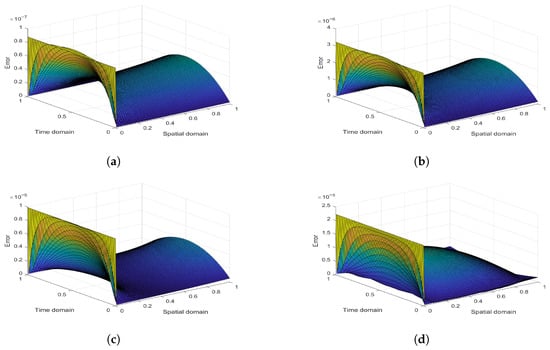
Figure 1. Surface Plots of AE with $dt=0.01$, $\gamma =0.001$, $\varpi =15$, $h=0.01$, and $ϵ=1$: (a) $\delta =1$, (b) $\delta =2$, (c) $\delta =3$, (d) $\delta =5$ for Example 1.

Table 5. The convergence order for different $dt$ and at fixed $h=0.01$.

$\mathit{d}\mathit{t}$	${\mathit{L}}_2$	${\mathit{L}}_{\mathit{\infty }}$	ROC	S.R
0.05	1.027E-07	1.300E-07		5.115E-04
0.025	8.740E-08	1.144E-07	0.18422	5.123E-04
0.016	8.186E-08	1.087E-07	0.11475	5.135E-04
0.01	7.817E-08	1.048E-07	0.07650	5.152E-04

5.2. Example 2

Consider Equations (2)–(4) with $d\mathrm{t}=0.01$, $h=0.01$. In Figure 2a–d, for various values of $ϵ$, $\delta =1$, $\varpi =1$, and $\gamma =0.001$, a comparison between the exact and CBS solutions is displayed. Figure 3a–d, shows the surface plot of the NS for various values of $ϵ$. In Figure 4a,b, Comparison for $ϵ={10}^{-10},{10}^{-20}$, $\delta =5$ and $\gamma =0.0001$ is shown. In this case, $d\mathrm{t}=0.1$, and $N=30$. Each plot makes it clear that when the $ϵ$ declines, the boundary layer becomes sharper. Figure 5 shows the surface plots for two different values of $ϵ$.

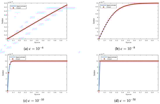
Figure 2. $u_E$ vs. $u_A$ for Example 2 with $dt=0.01$, $h=0.01$, $\gamma =0.001$, $\varpi =1$, and $\delta =1$.

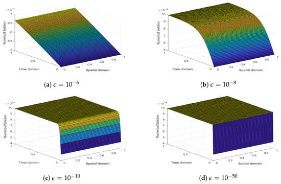
Figure 3. Surface plots of $u_A$ for Example 2.

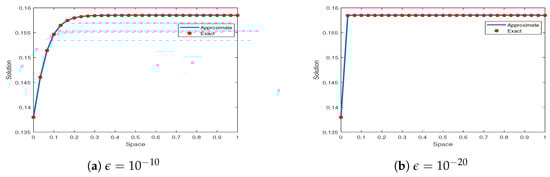
Figure 4. $u_E$ vs. $u_A$ for Example 2 ($dt=0.1$, $N=30$, $\gamma =0.0001$, $\varpi =1$, $\delta =5$).

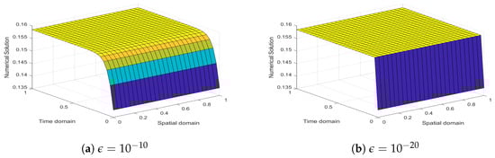
Figure 5. Surface plots for different values of $ϵ$ for Example 2.

5.3. Example 3

Consider Equations (2)–(4) where $ϵ=1$, $\varpi =1$, and various values of $\gamma$ and $\delta$. A comparison between $L_2$ and $L_{\infty }$ for $\gamma =0.001$ and $\delta =1,2$ with [27] is provided in Table 6 and Table 7, which shows the superiority of our results over the ISF-Galerkin method (ISF-Gm1,2) and the collocation method mixed with finite difference (MFDCM) [27]. Similarly, comparisons of $L_2$ and $L_{\infty }$ for $\gamma =0.0001$ and various values of $\delta =1,2$ are presented in Table 8 and Table 9, respectively. Table 10 shows $L_2$ and $L_{\infty }$ error norms for different temporal sizes. The (S.R) shows that the given method is stable, and the ROC gives the convergence of the proposed scheme.

Table 6. Errors comparison for Example 3 ($ϵ=1$, $\gamma =0.001$, $\varpi =1$, and $\delta =1$).

	Present Method		ISF-Gm1 [27]		ISF-Gm2 [27]		MFDCM [27]
t	${\mathit{L}}_{\mathbf{2}}$	${\mathit{L}}_{\infty }$	${\mathit{L}}_{\mathbf{2}}$	${\mathit{L}}_{\infty }$	${\mathit{L}}_{\mathbf{2}}$	${\mathit{L}}_{\infty }$	${\mathit{L}}_{\mathbf{2}}$	${\mathit{L}}_{\infty }$
0.3	0.248E-10	0.327E-10	0.431E-09	0.592E-09	0.324E-09	0.421E-09	0.433E-09	0.750E-09
0.6	0.258E-10	0.339E-10	0.455E-09	0.623E-09	0.295E-09	0.411E-09	0.455E-09	0.782E-09
1	0.331E-10	0.434E-10	0.456E-09	0.624E-09	0.287E-09	0.449E-09	0.456E-09	0.784E-09

Table 7. Comparison of errors for $ϵ=1$, $\gamma =0.001$, $\varpi =1$, and $\delta =2$ of Example 3.

	Present Method		ISF-Gm1 [27]		ISF-Gm2 [27]		MFDCM [27]
t	${\mathit{L}}_{\mathbf{2}}$	${\mathit{L}}_{\infty }$	${\mathit{L}}_{\mathbf{2}}$	${\mathit{L}}_{\infty }$	${\mathit{L}}_{\mathbf{2}}$	${\mathit{L}}_{\infty }$	${\mathit{L}}_{\mathbf{2}}$	${\mathit{L}}_{\infty }$
0.3	0.654E-08	0.885E-08	0.193E-07	0.265E-07	0.154E-07	0.203E-07	0.193E-07	0.322E-07
0.6	0.759E-08	0.101E-07	0.203E-07	0.278E-07	0.145E-07	0.201E-07	0.203E-07	0.337E-07
1	0.124E-07	0.165E-07	0.204E-07	0.279E-07	0.141E-07	0.215E-07	0.204E-07	0.337E-07

Table 8. Comparison of errors for $ϵ=1$, $\gamma =0.0001$, $\varpi =1$, and $\delta =1$ of Example 3.

	Present Method		ISF-Gm1 [27]		ISF-Gm2 [27]		MFDCM [27]
t	${\mathit{L}}_{\mathbf{2}}$	${\mathit{L}}_{\infty }$	${\mathit{L}}_{\mathbf{2}}$	${\mathit{L}}_{\infty }$	${\mathit{L}}_{\mathbf{2}}$	${\mathit{L}}_{\infty }$	${\mathit{L}}_{\mathbf{2}}$	${\mathit{L}}_{\infty }$
0.3	0.261E-12	0.355E-12	0.432E-11	0.592E-11	0.323E-11	0.423E-11	0.434E-11	0.752E-11
0.6	0.272E-12	0.367E-12	0.454E-11	0.623E-11	0.296E-11	0.412E-11	0.456E-11	0.782E-11
1	0.350E-12	0.472E-12	0.456E-11	0.625E-11	0.288E-11	0.448E-11	0.456E-11	0.785E-11

Table 9. Comparison of errors for $ϵ=1$, $\gamma =0.0001$, $\varpi =1$, and $\delta =2$ of Example 3.

	Present Method		ISF-Gm1 [27]		ISF-Gm2 [27]		MFDCM [27]
t	${\mathit{L}}_{\mathbf{2}}$	${\mathit{L}}_{\infty }$	${\mathit{L}}_{\mathbf{2}}$	${\mathit{L}}_{\infty }$	${\mathit{L}}_{\mathbf{2}}$	${\mathit{L}}_{\infty }$	${\mathit{L}}_{\mathbf{2}}$	${\mathit{L}}_{\infty }$
0.3	0.208E-09	0.281E-09	0.610E-09	0.737E-09	0.487E-09	0.641E-09	0.612E-09	0.102E-08
0.6	0.241E-09	0.322E-09	0.643E-09	0.881E-09	0.459E-09	0.636E-09	0.644E-09	0.106E-08
1	0.392E-09	0.524E-09	0.645E-09	0.883E-09	0.446E-09	0.681E-09	0.645E-09	0.107E-08

Table 10. $L_2$ and $L_{\infty }$ norms along with rate of convergence and spectral radius at fixed $h=0.01$.

$\mathbf{dt}$	${\mathit{L}}_2$	${\mathit{L}}_{\mathit{\infty }}$	ROC	S.R
0.2	1.913E-09	2.155E-09		5.409E-05
0.1	1.336E-09	1.599E-09	0.43068	5.460E-05
0.08	1.215E-09	1.481E-09	0.34340	5.477E-05
0.04	9.682E-10	1.237E-09	0.25913	5.575E-05
0.01	8.442E-10	1.112E-09	0.15455	5.842E-05

5.4. Example 4

HH successfully simulates various neural behaviors; however, its complexity, involving a number of dynamic variables, produces challenges for network simulations. To overcome this, Fitzhugh [28] In 1961, they proposed the Fitzhugh–Nagumo neuron (FHN), which Nagumo, along with their co-workers, refined in 1962 [29]. It is the streamlined version of the HH model. The FHN focuses on the basic aspects of the excitable systems and provides insights into threshold behavior, recovery process, and oscillations. Now by taking $ϵ=\varpi =\delta =1$ in Equation (2), we obtain the FH equation, given as

$${\displaystyle \frac{\partial \mathrm{u}}{\partial \mathrm{t}}}-{\displaystyle \frac{{\partial }^2\mathrm{u}}{\partial {\zeta }^2}}=\mathrm{u}(1-\mathrm{u})(\mathrm{u}-\gamma ),\zeta \in (a,b),\mathrm{t}\ge 0,$$

(33)

The exact solution is

$$u(\zeta ,\mathrm{t})={\displaystyle \frac{1}{2}}+{\displaystyle \frac{1}{2}}tanh\left[{\displaystyle \frac{1}{2\sqrt{2}}}\left(\zeta -{\displaystyle \frac{2\gamma -1}{\sqrt{2}}}\mathrm{t}\right)\right].$$

(34)

The associated initial and boundary conditions are

$$\begin{array}{cc}\hfill u(\zeta ,0)& ={\displaystyle \frac{1}{2}}+{\displaystyle \frac{1}{2}}tanh\left({\displaystyle \frac{\zeta }{2\sqrt{2}}}\right),\hfill \\ \hfill u(a,\mathrm{t})& ={\displaystyle \frac{1}{2}}+{\displaystyle \frac{1}{2}}tanh\left[{\displaystyle \frac{1}{2\sqrt{2}}}\left(a-{\displaystyle \frac{2\gamma -1}{\sqrt{2}}}\mathrm{t}\right)\right],\hfill \\ \hfill u(b,\mathrm{t})& ={\displaystyle \frac{1}{2}}+{\displaystyle \frac{1}{2}}tanh\left[{\displaystyle \frac{1}{2\sqrt{2}}}\left(b-{\displaystyle \frac{2\gamma -1}{\sqrt{2}}}\mathrm{t}\right)\right].\hfill \end{array}$$

(35)

$\zeta \in [-1,1]$ and $\mathrm{t}\in [0,1]$. Table 11 and Table 12 are given at various times and $\gamma =0.4$. The time step size is $0.001$ and $0.0001$, respectively, and $h=0.1$. The results of CBS are compared with the septic B-Spline (SBS) using $L_2$ and $L_{\infty }$ error norms. As SBS required a lot of computational work and computational time. Furthermore, additional spline conditions are required in SBS to obtain a consistent algebraic system, which are obtained by taking the derivatives of the initial and boundary conditions; still, the results clearly show that CBS outperforms SBS. In Table 13, the $L_2$ and $L_{\infty }$ error norms for $dt=0.0001$, $h=0.1$ and $\gamma =0.7$. Figure 6 displays the exact and CBS comparison, which concludes that both are in good agreement. The results show that CBS is efficient and more reliable to deal with the neurodynamical models.

Table 11. Error values $L_2$ and $L_{\infty }$ at various times for $dt=0.001$ and $\gamma =0.4$.

$\mathit{dt}=0.001,\mathit{h}=0.1,\mathit{\gamma }=0.4$
$\mathrm{t}$	${\mathit{L}}_{\mathbf{2}}$	[30]	${\mathit{L}}_{\infty }$	[30]
0.01	1.1030E-05	6.797E-03	2.2125E-05	3.500E-03
0.02	1.2083E-05	1.359E-02	2.2133E-05	6.999E-03
0.03	1.2864E-05	2.039E-02	2.2140E-05	1.050E-02
0.04	1.3497E-05	2.719E-02	2.2148E-05	1.400E-02
0.05	1.4035E-05	3.398E-02	2.2155E-05	1.749E-02
0.1	1.5994E-05	6.796E-02	2.2192E-05	3.498E-02
1	3.1715E-05	6.796E-01	2.3511E-05	3.363E-01

Table 12. Error values $L_2$ and $L_{\infty }$ at various times for $dt=0.0001$ and $\gamma =0.4$.

$\mathit{dt}=0.0001,\mathit{h}=0.1,\mathit{\gamma }=0.4$
$\mathrm{t}$	${\mathit{L}}_{\mathbf{2}}$	[30]	${\mathit{L}}_{\infty }$	[30]
0.01	1.1291E-06	4.1173E-05	2.2126E-06	6.528E-05
0.02	1.2757E-06	7.8889E-05	2.2133E-06	1.017E-04
0.03	1.4060E-06	1.1690E-04	2.2141E-06	1.366E-04
0.04	2.2148E-06	1.5503E-04	2.2148E-06	1.710E-04
0.05	1.6372E-06	1.9329E-04	2.2156E-06	2.054E-04
1	5.1024E-06	6.5867E-03	5.1024E-06	6.611E-03

Table 13. Error values $L_2$ and $L_{\infty }$ at various times for $dt=0.0001$ and $\gamma =0.7$.

$\mathit{dt}=0.0001,\mathit{h}=0.1,\mathit{\gamma }=0.7$
$\mathrm{t}$	${\mathit{L}}_{\mathbf{2}}$	[30]	${\mathit{L}}_{\infty }$	[30]
0.01	2.2273E-06	4.12E-05	4.4266E-06	6.53E-05
0.02	2.4561E-06	7.89E-05	4.4296E-06	1.02E-04
0.03	2.6380E-06	1.17E-04	4.4326E-06	1.37E-04
0.04	2.7939E-06	1.55E-04	4.4356E-06	1.71E-04
0.05	2.9323E-06	1.93E-04	4.4386E-06	2.05E-04
1	8.8243E-06	6.59E-03	8.0353E-06	6.61E-03

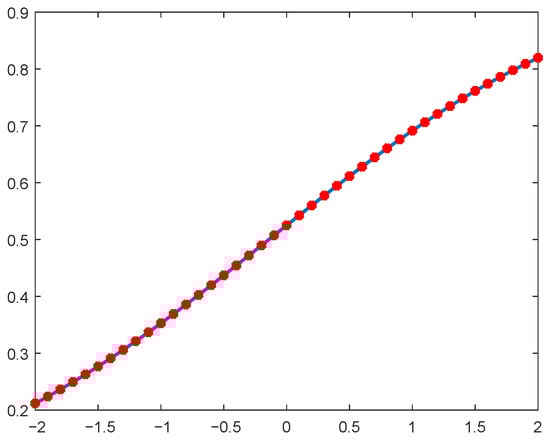
Figure 6. Exact vs. approximate 2D plot at $dt=0.01$.

6. Conclusions

This work uses the CBSCM to solve the singularly perturbed generalized HH problem. To evaluate the effectiveness of the current approach, several examples are discussed. The CBS approach yields findings that are consistent with the exact answers. When compared to conventional finite difference and collocation techniques documented in the literature, the results show enhanced accuracy and stability. These findings show how effective and powerful this approach is for numerically analyzing a wide range of complex nonlinear PDEs. The Von Neumann stability of the proposed method and spectral radius showed that it is unconditionally stable. Overall, the proposed technique proved to be an efficient, accurate, and mesh-based approach for solving neurodynamical models and holds strong potential for future extensions to nonlinear, and fractional problems.

References

- Cavaterra, C.; Grasselli, M. Robust Exponential Attractors for Singularly Perturbed Hodgkin–Huxley Equations. J. Differ. Equ. 2009, 246, 4670–4701. [Google Scholar] [CrossRef]
- Evans, J.; Shenk, N. Solutions to Axon Equations. Biophys. J. 1970, 10, 1090–1101. [Google Scholar] [CrossRef]
- Hashim, I.; Noorani, M.S.M.; Batiha, B. A Note on the Adomian Decomposition Method for the Generalized Huxley Equation. Appl. Math. Comput. 2006, 181, 1439–1445. [Google Scholar] [CrossRef]
- Batiha, B.; Noorani, M.S.M.; Hashim, I. Numerical Simulation of the Generalized Huxley Equation by He’s Variational Iteration Method. Appl. Math. Comput. 2007, 186, 1322–1325. [Google Scholar] [CrossRef]
- Sangwan, V.; Kumar, B.V.R.; Murthy, S.V.S.S.N.V.G.K.; Nigam, M. Three-Step Taylor Galerkin Method for Singularly Perturbed Generalized Hodgkin–Huxley Equation. Int. J. Model. Simul. Sci. Comput. 2010, 1, 257–276. [Google Scholar] [CrossRef]
- Aderogba, A.A.; Chapwanya, M. Positive and Bounded Nonstandard Finite Difference Scheme for the Hodgkin–Huxley Equations. Jpn. J. Ind. Appl. Math. 2018, 35, 773–785. [Google Scholar] [CrossRef]
- Macías-Díaz, J.E.; Ruiz-Ramírez, J.; Villa, J. The Numerical Solution of a Generalized Burgers–Huxley Equation through a Conditionally Bounded and Symmetry-Preserving Method. Comput. Math. Appl. 2011, 61, 3330–3342. [Google Scholar] [CrossRef]
- Sari, M.; Gürarslan, G.; Zeytinoğlu, A. High-Order Finite Difference Schemes for Numerical Solutions of the Generalized Burgers–Huxley Equation. Numer. Methods Part. Differ. Equ. 2011, 27, 1313–1326. [Google Scholar] [CrossRef]
- Kaushik, A.; Sharma, M.D. A Uniformly Convergent Numerical Method on Non-Uniform Mesh for Singularly Perturbed Unsteady Burger–Huxley Equation. Appl. Math. Comput. 2008, 195, 688–706. [Google Scholar] [CrossRef]
- Batiha, B.; Noorani, M.S.M.; Hashim, I. Application of Variational Iteration Method to the Generalized Burgers–Huxley Equation. Chaos Solitons Fractals 2008, 36, 660–663. [Google Scholar] [CrossRef]
- El-Kady, M.; El-Sayed, S.M.; Fathy, H.E. Development of Galerkin Method for Solving the Generalized Burger’s–Huxley Equation. Math. Probl. Eng. 2013, 2013, 165492. [Google Scholar] [CrossRef]
- Roos, H.G.; Stynes, M.; Tobiska, L. Robust Numerical Methods for Singularly Perturbed Differential Equations; Springer: Berlin/Heidelberg, Germany, 2008. [Google Scholar]
- Jain, M.K.; Iyengar, S.R.K.; Jain, R.K. Numerical Methods for Scientific and Engineering Computation; New Age International: New Delhi, India, 1997. [Google Scholar]
- Talwar, J.; Mohanty, R.K. Spline in tension method for nonlinear two-point boundary value problems on a geometric mesh. Math. Model. 2015, 27, 33–48. [Google Scholar]
- Rubin, S.G.; Khosla, P.K. Higher-order numerical solutions using cubic splines. AIAA J. 1977, 15, 421–424. [Google Scholar] [CrossRef]
- Qiao, B.; Chen, X.; Xue, X.; Luo, X.; Liu, R. The Application of Cubic B-Spline Collocation Method in Impact Force Identification. Mech. Syst. Signal Process. 2015, 64, 413–427. [Google Scholar] [CrossRef]
- Yousafzai, A.; Haq, S.; Ghafoor, A.; Shah, K.; Abdeljawad, T. Solution of the Foam-Drainage Equation with Cubic B-Spline Hybrid Approach. Phys. Scr. 2024, 99, 075279. [Google Scholar] [CrossRef]
- Iqbal, A.; Abd Hamid, N.N.; Md. Ismail, A.I. Soliton solution of Schrödinger equation using cubic B-spline Galerkin method. Fluids 2019, 4, 108. [Google Scholar] [CrossRef]
- Botella, O. On a Collocation B-Spline Method for the Solution of the Navier–Stokes Equations. Comput. Fluids 2002, 31, 397–420. [Google Scholar] [CrossRef]
- Akbar, T.; Haq, S.; Arifeen, S.U.; Iqbal, A. Numerical Solution of Third-Order Rosenau–Hyman and Fornberg–Whitham Equations via B-Spline Interpolation Approach. Axioms 2024, 13, 501. [Google Scholar] [CrossRef]
- Singh, A.; Dahiya, S.; Singh, S.P. A Fourth-Order B-Spline Collocation Method for Nonlinear Burgers–Fisher Equation. Math. Sci. 2020, 14, 75–85. [Google Scholar] [CrossRef]
- Dağ, İ.; Saka, B. A Cubic B-Spline Collocation Method for the EW Equation. Math. Comput. Appl. 2004, 9, 381–392. [Google Scholar] [CrossRef]
- Tamsir, M.; Dhiman, N.; Chauhan, A.; Chauhan, A. Solution of Parabolic PDEs by Modified Quintic B-Spline Crank–Nicolson Collocation Method. Ain Shams Eng. J. 2021, 12, 2073–2082. [Google Scholar] [CrossRef]
- Dhiman, N.; Tamsir, M.; Chauhan, A.; Nigam, D. An Implicit Collocation Algorithm Based on Cubic Extended B-Splines for Caputo Time-Fractional PDE. Mater. Today Proc. 2021, 46, 11094–11097. [Google Scholar] [CrossRef]
- Dhiman, N.; Huntul, M.J.; Tamsir, M. A Modified Trigonometric Cubic B-Spline Collocation Technique for Solving the Time-Fractional Diffusion Equation. Eng. Comput. 2021, 38, 2921–2936. [Google Scholar] [CrossRef]
- Tamsir, M.; Dhiman, N.; Nigam, D.; Chauhan, A. Approximation of Caputo Time-Fractional Diffusion Equation Using Redefined Cubic Exponential B-Spline Collocation Technique. AIMS Math. 2021, 6, 3805–3820. [Google Scholar] [CrossRef]
- Dehghan, M.; Nemati-Saray, B.; Lakestani, M. Three Methods Based on Interpolation Scaling Functions and Mixed Collocation Finite Difference Schemes for the Nonlinear Generalized Burgers–Huxley Equation. Math. Comput. Model. 2012, 55, 1129–1142. [Google Scholar] [CrossRef]
- FitzHugh, R. Impulses and physiological states in theoretical models of nerve membrane. Biophys. J. 1961, 1, 445–466. [Google Scholar] [CrossRef] [PubMed]
- Nagumo, J.; Arimoto, S.; Yoshizawa, S. An active pulse transmission line simulating nerve axon. Proc. IRE 1962, 50, 2061–2070. [Google Scholar] [CrossRef]
- Sucu, D.Y.; Karakoç, S.B.G.; Güngör, M. Investigation on the new numerical soliton solutions of FitzHugh–Nagumo equation with collocation method. Fundam. J. Math. Appl. 2025, 8, 180–186. [Google Scholar] [CrossRef]
Disclaimer/Publisher’s Note: The statements, opinions and data contained in all publications are solely those of the individual author(s) and contributor(s) and not of MDPI and/or the editor(s). MDPI and/or the editor(s) disclaim responsibility for any injury to people or property resulting from any ideas, methods, instructions or products referred to in the content. |
© 2025 by the authors. Licensee MDPI, Basel, Switzerland. This article is an open access article distributed under the terms and conditions of the Creative Commons Attribution (CC BY) license.