Efficient Layer-Resolving Fitted Mesh Finite Difference Approach for Solving a System of n Two-Parameter Singularly Perturbed Convection–Diffusion Delay Differential Equations

Abstract

This paper presents a robust fitted mesh finite difference method for solving a system of n singularly perturbed two parameter convection–reaction–diffusion delay differential equations defined on the interval $[0,2]$. Leveraging a piecewise uniform Shishkin mesh, the method adeptly captures the solution’s behavior arising from delay term and small perturbation parameters. The proposed numerical scheme is rigorously analyzed and proven to be parameter-robust, exhibiting nearly first-order convergence. A numerical illustration is included to validate the method’s efficiency and to confirm the theoretical predictions.

1. Introduction

Singularly perturbed differential equations (SPDEs) are integral to many fields, including fluid dynamics, chemical reactor theory, population dynamics and control systems [1,2]. Within this class, singularly perturbed delay differential equations (SPDDEs) present additional complexities due to boundary and interior layers that arise from small perturbation parameters and delay terms, making numerical solutions challenging. Established techniques like fitted mesh [3] and fitted operator methods [4] have provided accurate solutions for SPDEs, such as within the work of Cen [5], who used a hybrid scheme with a Shishkin mesh to achieve near-second-order convergence. Similarly, Gracia et al. [6] developed a monotone method for SPDEs with two parameters influencing convection and diffusion. SPDDEs typically involve boundary value problems influenced by two small parameters, $\mu$ and ${ϵ}_i(i=1,2,\cdots ,n)$, whose interactions generate complex layer behavior governed by the ratio ${\mu }^2/{ϵ}_i$. This work aims to construct a parameter-robust numerical method for a system of n SPDDEs as both parameters approach zero, addressing boundary and interior layers accurately regardless of perturbation values. Stability is established, and bounds for the solution’s derivatives are derived, supporting the convergence of the fitted mesh finite difference approach, which attains nearly first-order accuracy. Numerous studies have explored singular perturbation problems, emphasizing their asymptotic behavior, the development of parameter uniform methods and challenges in introduced delay differential equations to achieve robust and accurate solutions across varying perturbation parameters [7,8,9,10,11,12]. The novelty of this research lies in addressing a system of n SPDDEs involving two small parameters in a convection–diffusion context, contrasting with prior studies that either considered single delay equations [13], a system of two equations without delay terms [14] and a system of two equations with delay terms [15]. This paper considers interacting variables affected by both delay and two distinct small perturbation parameters, ${ϵ}_i(i=1,2,\cdots ,n)$ and $\mu$, introducing challenges in boundary and interior layer formation. To overcome these challenges, this paper presents advanced mesh techniques and robust numerical schemes that effectively resolve layers and achieve parameter uniform convergence, significantly enhancing the numerical analysis of SPDDEs.

2. Formulation of the Problem

The following system of singularly perturbed delay differential equations involving two small parameters is under consideration:

$$E{\overrightarrow{\mathfrak{u}}}^{\prime \prime }\left(\varkappa \right)+\mu \mathcal{A}\left(\varkappa \right){\overrightarrow{\mathfrak{u}}}^{\prime }\left(\varkappa \right)-\mathcal{B}\left(\varkappa \right)\overrightarrow{\mathfrak{u}}\left(\varkappa \right)+\mathcal{D}\left(\varkappa \right)\overrightarrow{\mathfrak{u}}(\varkappa -1)=\overrightarrow{\mathit{f}}\left(\varkappa \right)\mathrm{for}\mathrm{all}\varkappa \in \mathrm{\Omega }=(0,2),$$

(1)

$$\overrightarrow{\mathfrak{u}}=\overrightarrow{\phi }\mathrm{on}[-1,0],\overrightarrow{\mathfrak{u}}\left(2\right)=\overrightarrow{\iota }.$$

Here, $\overrightarrow{\mathfrak{u}}=\left(\begin{array}{c}{\mathfrak{u}}_1\\ {\mathfrak{u}}_2\\ ⋮\\ {\mathfrak{u}}_n\end{array}\right),\overrightarrow{\mathit{f}}=\left(\begin{array}{c}{f}_1\\ f_2\\ ⋮\\ f_n\end{array}\right),$ $E=\left(\begin{array}{cccc}{ϵ}_1& 0& \cdots & 0\\ 0& {ϵ}_2& \cdots & 0\\ ⋮& ⋮& \ddots & ⋮\\ 0& 0& \cdots & {ϵ}_n\end{array}\right),\mathcal{A}\left(\varkappa \right)=\left(\begin{array}{cccc}{\mathfrak{a}}_1\left(\varkappa \right)& 0& \cdots & 0\\ 0& {\mathfrak{a}}_2\left(\varkappa \right)& \cdots & 0\\ ⋮& ⋮& \ddots & ⋮\\ 0& 0& \cdots & {\mathfrak{a}}_n\left(\varkappa \right)\end{array}\right),$ $\mathcal{B}\left(\varkappa \right)=\left(\begin{array}{cccc}{\mathfrak{b}}_{11}\left(\varkappa \right)& -{\mathfrak{b}}_{12}\left(\varkappa \right)& \cdots & -{\mathfrak{b}}_{1n}\left(\varkappa \right)\\ -{\mathfrak{b}}_{21}\left(\varkappa \right)& {\mathfrak{b}}_{22}\left(\varkappa \right)& \cdots & -{\mathfrak{b}}_{2n}\left(\varkappa \right)\\ ⋮& ⋮& \ddots & ⋮\\ -{\mathfrak{b}}_{n1}\left(\varkappa \right)& -{\mathfrak{b}}_{n2}\left(\varkappa \right)& \cdots & {\mathfrak{b}}_{nn}\left(\varkappa \right)\end{array}\right),$ $\mathcal{D}\left(\varkappa \right)=\left(\begin{array}{cccc}{\mathfrak{d}}_1\left(\varkappa \right)& 0& \cdots & 0\\ 0& {\mathfrak{d}}_2\left(\varkappa \right)& \cdots & 0\\ ⋮& ⋮& \ddots & ⋮\\ 0& 0& \cdots & {\mathfrak{d}}_n\left(\varkappa \right)\end{array}\right),$ where ${ϵ}_i$,$i=1,2,\cdots ,n$ are small parameters satisfying $0<{ϵ}_1<{ϵ}_2<\cdots <{ϵ}_n\le 1$, and $\mu$ is another small parameter with $0<\mu \le 1$. The coefficient functions ${\mathfrak{a}}_i\left(\varkappa \right)$, ${\mathfrak{b}}_{ij}\left(\varkappa \right)$, ${\mathfrak{d}}_i\left(\varkappa \right)$ and $f_i\left(\varkappa \right)$ are all sufficiently smooth throughout the domain $\overline{\mathrm{\Omega }}=[0,2]$ and ${\mathfrak{a}}_i\left(\varkappa \right)\ge \alpha >0,{\mathfrak{b}}_{ii}\left(\varkappa \right)+{\sum }_{j=1}^n{\mathfrak{b}}_{ij}\left(\varkappa \right)\ge \beta >0,{\mathfrak{d}}_i\left(\varkappa \right)>0,$ ${\mathfrak{b}}_{ii}\left(\varkappa \right)+{\sum }_{j=1}^n{\mathfrak{b}}_{ij}\left(\varkappa \right)-{\mathfrak{d}}_i\left(\varkappa \right)\ge \kappa >0,\mathrm{for}i,j=1,2,\cdots ,n\mathrm{and}i\ne j.$ The $\overrightarrow{\phi }\left(x\right)$ is sufficiently smooth over the interval $[-1,0]$. The value of $\gamma$ is determined as $\gamma ={min}_{\varkappa \in \overline{\mathrm{\Omega }}}\left({\displaystyle \frac{{\sum }_{j=1}^n{\mathfrak{b}}_{ij}\left(\varkappa \right)-{\mathfrak{d}}_i\left(\varkappa \right)}{{\mathfrak{a}}_i\left(\varkappa \right)}}\right)\mathrm{for}i=1,2,\cdots ,n\mathrm{and}i\ne j.$ When $\mu =0$, the above problem without a delay term has been considered in [16]. The problem demonstrates boundary layers influenced by both ${ϵ}_i$ and $\mu$; in particular, the layers are influenced by the ratio of ${\displaystyle \frac{{\mu }^2}{{ϵ}_i}}$. If ${\displaystyle \frac{{\mu }^2}{{ϵ}_i}}\le {\displaystyle \frac{\gamma }{\alpha }}$, $1\le i\le n$, the reduced problem can be expressed as

$$-\mathcal{B}\left(\varkappa \right)\overrightarrow{\mathfrak{u}}\left(\varkappa \right)+\mathcal{D}\left(\varkappa \right)\overrightarrow{\mathfrak{u}}(\varkappa -1)=\overrightarrow{\mathit{f}}\left(\varkappa \right),\varkappa \in (0,2],$$

(2)

with boundary conditions $\overrightarrow{\mathfrak{u}}\left(\varkappa \right)=\overrightarrow{\phi }\left(\varkappa \right)\mathrm{on}[-1,0].$ This predicts that there will be a boundary layer of width $O\left(\sqrt{{ϵ}_i}\right)$ near $\varkappa =0$ and an interior layer at $\varkappa =1$, arising from the unit delay component, under the assumption that $\overrightarrow{\mathfrak{u}}\left(0\right)\ne \overrightarrow{\phi }\left(0\right)$. Additionally, a similar boundary layer of width $O\left(\sqrt{{ϵ}_i}\right)$ is anticipated near $\varkappa =2$, along with an interior layer at $\varkappa =1$, if $\overrightarrow{\mathfrak{u}}\left(2\right)\ne \overrightarrow{\iota }$. If ${\displaystyle \frac{{\mu }^2}{{ϵ}_j}}\ge {\displaystyle \frac{\gamma }{\alpha }}$, $1<i<j\le n$, the reduced problem is

$$\mu \mathcal{A}\left(\varkappa \right){\overrightarrow{\mathfrak{u}}}^{\prime }\left(\varkappa \right)-\mathcal{B}\left(\varkappa \right)\overrightarrow{\mathfrak{u}}\left(\varkappa \right)+\mathcal{D}\left(\varkappa \right)\overrightarrow{\mathfrak{u}}(\varkappa -1)=\overrightarrow{\mathit{f}}\left(\varkappa \right),\varkappa \in (0,2),$$

(3)

with boundary conditions $\overrightarrow{\mathfrak{u}}\left(\varkappa \right)=\overrightarrow{\phi }\left(\varkappa \right)\mathrm{on}[-1,0],\overrightarrow{\mathfrak{u}}\left(2\right)=\overrightarrow{\iota }.$ This problem remains to exhibit singular perturbation behavior due to the parameter $\mu$. It is expected that a boundary layer with a width $O\left(\mu \right)$ is anticipated near $\varkappa =2$, and an interior layer at $\varkappa =1$ (due to the delay), unless the solution at $\varkappa =2$ differs from $\overrightarrow{\iota }$. Additionally, a boundary layer of width $O\left({\displaystyle \frac{{ϵ}_i}{\mu }}\right)$ is anticipated near $\varkappa =0$, with an interior layer at $\varkappa =1$, if $\overrightarrow{\mathfrak{u}}\left(0\right)\ne \overrightarrow{\phi }\left(0\right)$. Numerical experiments indicate that the interior right layer weakens considerably when ${ϵ}_i\ll {\mu }^2$. Consider the problem

$${\overrightarrow{L}}_1\overrightarrow{\mathit{z}}\left(\varkappa \right)=E{\overrightarrow{\mathit{z}}}^{\prime \prime }\left(\varkappa \right)+\mu \mathcal{A}\left(\varkappa \right){\overrightarrow{\mathit{z}}}^{\prime }\left(\varkappa \right)-\mathcal{B}\left(\varkappa \right)\overrightarrow{\mathit{z}}\left(\varkappa \right)=\overrightarrow{\mathcal{g}}\left(\varkappa \right),\varkappa \in {\mathrm{\Omega }}_1,$$

(4)

$${\overrightarrow{L}}_2\overrightarrow{\mathit{z}}\left(\varkappa \right)=E{\overrightarrow{\mathit{z}}}^{\prime \prime }\left(\varkappa \right)+\mu \mathcal{A}\left(\varkappa \right){\overrightarrow{\mathit{z}}}^{\prime }\left(\varkappa \right)-\mathcal{B}\left(\varkappa \right)\overrightarrow{\mathit{z}}\left(\varkappa \right)+\mathcal{D}\left(\varkappa \right)\overrightarrow{\mathit{z}}(\varkappa -1)=\overrightarrow{\mathit{f}}\left(\varkappa \right),\varkappa \in {\mathrm{\Omega }}_2,$$

(5)

with boundary conditions $\overrightarrow{\mathit{z}}\left(0\right)=\overrightarrow{\phi }\left(0\right),\overrightarrow{\mathit{z}}(1-)=\overrightarrow{\mathit{z}}(1+),{\overrightarrow{\mathit{z}}}^{\prime }(1-)={\overrightarrow{\mathit{z}}}^{\prime }(1+),\overrightarrow{\mathit{z}}\left(2\right)=\overrightarrow{\iota },$ where $\overrightarrow{\mathcal{g}}\left(\varkappa \right)=\overrightarrow{\mathit{f}}\left(\varkappa \right)-\mathcal{D}\left(\varkappa \right)\overrightarrow{\phi }(\varkappa -1),$ for $\varkappa \in {\mathrm{\Omega }}_1$, ${\mathrm{\Omega }}_1=(0,1)$ and ${\mathrm{\Omega }}_2=(1,2)$.

3. Analytical Results

This section presents a minimum principle, establishes a stability result for the problem described by Equation (1) and provides its estimates for the derivatives of the solution.

Lemma 1.

Let $\overrightarrow{\mathit{\psi }}={({\mathit{\psi }}_1,{\mathit{\psi }}_2,\cdots ,{\mathit{\psi }}_n)}^T$ be such that $\overrightarrow{\mathit{\psi }}\left(0\right)\ge \overrightarrow{0}$, $\overrightarrow{\mathit{\psi }}\left(2\right)\ge \overrightarrow{0}$, ${\overrightarrow{L}}_1\overrightarrow{\mathit{\psi }}\le \overrightarrow{0}$ on $(0,1)$ and ${\overrightarrow{L}}_2\overrightarrow{\mathit{\psi }}\le \overrightarrow{0}$ on $(1,2)$, $\overrightarrow{\mathit{\psi }}\left(1\right)=\overrightarrow{0}$, ${\overrightarrow{\mathit{\psi }}}^{\prime }\left(1\right)\le \overrightarrow{0}$; then, $\overrightarrow{\mathit{\psi }}\ge \overrightarrow{0}$ on $[0,2]$.

Proof. 

Assume that ${\varkappa }^{*}$ and $s^{*}$ are such that ${\displaystyle {\mathit{\psi }}_{s^{*}}\left({\varkappa }^{*}\right)=\underset{\varkappa \in \mathrm{\Omega },s=1,2,\cdots ,n}{min}{\mathit{\psi }}_s\left(\varkappa \right)}$. Suppose ${\mathit{\psi }}_{s^{*}}\left({\varkappa }^{*}\right)<0$. Then, ${\varkappa }^{*}$ cannot be at the boundaries 0 or 2. At ${\varkappa }^{*}$, the first derivative of ${\mathit{\psi }}_{s^{*}}$ is denoted as ${\mathit{\psi }}_{s^{*}}^{\prime }\left({\varkappa }^{*}\right)=0$ and the second derivative is denoted as ${\mathit{\psi }}_{s^{*}}^{\prime \prime }\left({\varkappa }^{*}\right)\ge 0$.

• Claim (i): ${\varkappa }^{*}\notin (0,1)$. If ${\varkappa }^{*}\in (0,1)$, then

  $${\left({\overrightarrow{L}}_1\overrightarrow{\mathit{\psi }}\right)}_{s^{*}}\left({\varkappa }^{*}\right)={ϵ}_{s^{*}}{\mathit{\psi }}_{s^{*}}^{\prime \prime }\left({\varkappa }^{*}\right)+\mu {\mathfrak{a}}_{s^{*}}\left({\varkappa }^{*}\right){\mathit{\psi }}_{s^{*}}^{\prime }\left({\varkappa }^{*}\right)-\sum _{j=1}^n{\mathfrak{b}}_{s^{*}j}\left({\varkappa }^{*}\right){\mathit{\psi }}_j\left({\varkappa }^{*}\right)>0,$$

  which contradicts the assumption that ${\overrightarrow{L}}_1\overrightarrow{\mathit{\psi }}\le \overrightarrow{0}$ on $(0,1)$. Thus, ${\varkappa }^{*}\notin (0,1)$.
• Claim (ii): ${\varkappa }^{*}\notin [1,2)$. If ${\varkappa }^{*}\in [1,2)$, then

  $${\left({\overrightarrow{L}}_2\overrightarrow{\mathit{\psi }}\right)}_{s^{*}}\left({\varkappa }^{*}\right)={ϵ}_{s^{*}}{\mathit{\psi }}_{s^{*}}^{\prime \prime }\left({\varkappa }^{*}\right)+\mu {\mathfrak{a}}_{s^{*}}\left({\varkappa }^{*}\right){\mathit{\psi }}_{s^{*}}^{\prime }\left({\varkappa }^{*}\right)-\sum _{j=1}^n\left[{\mathfrak{b}}_{s^{*}j}\left({\varkappa }^{*}\right)\right]{\mathit{\psi }}_j\left({\varkappa }^{*}\right)-{\mathfrak{d}}_{s^{*}}\left({\varkappa }^{*}\right){\mathit{\psi }}_{s^{*}}({\varkappa }^{*}-1)>0,$$

  which contradicts the assumption that ${\overrightarrow{L}}_2\overrightarrow{\mathit{\psi }}\le \overrightarrow{0}$ on $[1,2)$. Hence, ${\varkappa }^{*}\notin [1,2)$. When ${\varkappa }^{*}=1$, the differentiability of ${\mathit{\psi }}_{s^{*}}$ at $\varkappa =1$. If ${\mathit{\psi }}_{s^{*}}^{\prime }\left(1\right)$ does not exist, then ${\mathit{\psi }}_{s^{*}}^{\prime }\left(1\right)={\mathit{\psi }}_{s^{*}}^{\prime }(1+)-{\mathit{\psi }}_{s^{*}}^{\prime }(1-)>0$, which contradicts the condition ${\mathit{\psi }}_{s^{*}}^{\prime }\left(1\right)\le 0$. If ${\mathit{\psi }}_{s^{*}}$ is differentiable at $\varkappa =1$, then $\mu {\mathfrak{a}}_{s^{*}}\left(1\right){\mathit{\psi }}_{s^{*}}^{\prime }\left(1\right)-{\sum }_{j=1}^n{\mathfrak{b}}_{s^{*}j}\left(1\right){\mathit{\psi }}_j\left(1\right)>0.$ Since all entries of $\mathcal{A}\left(\varkappa \right)$, $\mathcal{B}\left(\varkappa \right)$ and ${\mathit{\psi }}_j\left(\varkappa \right)$ are continuous on $[0,2]$, there exists an interval $[1-h,1)$ where

  $$\mu {\mathfrak{a}}_{s^{*}}\left(\varkappa \right){\mathit{\psi }}_{s^{*}}^{\prime }\left(\varkappa \right)-\sum _{j=1}^n{\mathfrak{b}}_{s^{*}j}\left(\varkappa \right){\mathit{\psi }}_j\left(\varkappa \right)>0.$$

  Next, the second derivative ${\mathit{\psi }}_{s^{*}}^{\prime \prime }\left(\varkappa \right)$ is examined. If ${\mathit{\psi }}_{s^{*}}^{\prime \prime }\left(p\right)\ge 0$ for any $p\in [1-h,1)$, then ${\left({\overrightarrow{L}}_1\overrightarrow{\mathit{\psi }}\right)}_{s^{*}}\left(p\right)\ge 0$, which leads to a contradiction. Therefore, we assume ${\mathit{\psi }}_{s^{*}}^{\prime \prime }\left(\varkappa \right)<0$ on the interval $[1-h,1)$. This indicates that ${\mathit{\psi }}_{s^{*}}^{\prime }\left(\varkappa \right)$ is strictly decreasing over $[1-h,1)$. Given that ${\mathit{\psi }}_{s^{*}}^{\prime }\left(1\right)=0$ and ${\mathit{\psi }}_{s^{*}}^{\prime }$ is continuous on $(0,2)$, it follows that ${\mathit{\psi }}_{s^{*}}^{\prime }\left(\varkappa \right)>0$ on $[1-h,1)$. As a result, the continuous function ${\mathit{\psi }}_{s^{*}}\left(\varkappa \right)$ cannot attain a minimum at $\varkappa =1$, which contradicts the assumption that ${\varkappa }^{*}=1$. Thus, $\overrightarrow{\mathit{\psi }}\ge \overrightarrow{0}$ on $[0,2]$. The proof of the lemma is completed. □

Lemma 2

(Stability Result). Let $\overrightarrow{\mathit{\psi }}\in C^2\left(\overline{\mathrm{\Omega }}\right)$. For $\varkappa \in \overline{\mathrm{\Omega }}$,

$$|{\mathit{\psi }}_i\left(\varkappa \right)|\le max\left\{|\overrightarrow{\mathit{\psi }}\left(0\right)|,|\overrightarrow{\mathit{\psi }}\left(2\right)|,{\displaystyle \frac{1}{\kappa }}\parallel \overrightarrow{L_1}\overrightarrow{\mathit{\psi }}{\parallel }_{{\mathrm{\Omega }}_1},{\displaystyle \frac{1}{\kappa }}{\parallel \overrightarrow{L_2}\overrightarrow{\mathit{\psi }}\parallel }_{{\mathrm{\Omega }}_2}\right\}.$$

Proof. 

Define

$$M=max\left\{|\overrightarrow{\mathit{\psi }}\left(0\right)|,|\overrightarrow{\mathit{\psi }}\left(2\right)|,{\displaystyle \frac{1}{\kappa }}\parallel \overrightarrow{L_1}\overrightarrow{\mathit{\psi }}{\parallel }_{{\mathrm{\Omega }}_1},{\displaystyle \frac{1}{\kappa }}{\parallel \overrightarrow{L_2}\overrightarrow{\mathit{\psi }}\parallel }_{{\mathrm{\Omega }}_2}\right\}.$$

Consider the functions ${\overrightarrow{\theta }}^{\pm }\left(\varkappa \right)=M\overrightarrow{e}\pm \overrightarrow{\mathit{\psi }}\left(\varkappa \right)$, where $\overrightarrow{e}={(1,1,\cdots ,1)}^T$. Clearly, ${\overrightarrow{\theta }}^{\pm }\left(0\right)\ge \overrightarrow{0}$, ${\overrightarrow{\theta }}^{\pm }\left(2\right)\ge \overrightarrow{0}$, ${\overrightarrow{L}}_1{\overrightarrow{\theta }}^{\pm }\left(\varkappa \right)\le \overrightarrow{0}$ and ${\overrightarrow{L}}_2{\overrightarrow{\theta }}^{\pm }\left(\varkappa \right)\le \overrightarrow{0}$ for all $\varkappa \in \mathrm{\Omega }$. Hence, by Lemma 1, it is proven that $|{\mathit{\psi }}_i\left(\varkappa \right)|\le M$, which yields the required result. The proof of the lemma is completed. □

Theorem 1.

Let $\overrightarrow{u}$ be the solution of (1); then, its derivatives satisfy the following bounds on Ω:

$$|{\mathfrak{u}}_i^{\left(k\right)}\left(\varkappa \right)|\le {\displaystyle \frac{C}{{\left({\sqrt{ϵ}}_i\right)}^k}}\left(1+{\left({\displaystyle \frac{\mu }{\sqrt{{ϵ}_i}}}\right)}^k\right)max\{\parallel \overrightarrow{\mathfrak{u}}\parallel ,\parallel \overrightarrow{f}\parallel \},$$

(6)

$$\left|{{\mathfrak{u}}_i}^{\left(3\right)}\left(\varkappa \right)\right|\le {\displaystyle \frac{C}{{\left(\sqrt{{ϵ}_i}\right)}^3}}\left(1+{\left({\displaystyle \frac{\mu }{\sqrt{{ϵ}_i}}}\right)}^3\right)max\left\{\parallel \overrightarrow{\mathfrak{u}}\parallel ,\parallel \overrightarrow{f}\parallel ,\parallel {\overrightarrow{f}}^{\prime }\parallel \right\},$$

(7)

$$|{\mathfrak{u}}_i^{\left(4\right)}\left(\varkappa \right)|\le {\displaystyle \frac{C}{{\left(\sqrt{{ϵ}_i}\right)}^4}}\left(1+{\left({\displaystyle \frac{\mu }{\sqrt{{ϵ}_i}}}\right)}^4\right)max\left\{\parallel \overrightarrow{\mathfrak{u}}\parallel ,\parallel \overrightarrow{f}\parallel ,\parallel {\overrightarrow{f}}^{\prime }\parallel ,\parallel {\overrightarrow{f}}^{\prime \prime }\parallel \right\}$$

(8)

where the constant C is independent of ${ϵ}_i$ and μ, $i=1,2,\cdots ,n$ and $k=1,2$.

Proof. 

The proof follows the methodology outlined in Lemma 2.2 of [8]. For any $\varkappa \in (0,1)$, a neighborhood $N_p=(p,p+\sqrt{{ϵ}_i})$ such that $\varkappa \in N_p$ and $N_p\subset (0,1)$. According to the mean value theorem, there exists a $y\in N_p$ satisfying

$${\mathfrak{u}}_i^{\prime }\left(y\right)={\displaystyle \frac{{\mathfrak{u}}_i(p+\sqrt{{ϵ}_i})-{\mathfrak{u}}_i\left(p\right)}{\sqrt{{ϵ}_i}}}\Rightarrow |{\mathfrak{u}}_i^{\prime }\left(y\right)|\le {\displaystyle \frac{2\parallel {\mathfrak{u}}_i\parallel }{\sqrt{{ϵ}_i}}}.$$

Now, it follows that ${\mathfrak{u}}_i^{\prime }\left(\varkappa \right)={\mathfrak{u}}_i^{\prime }\left(y\right)+{\int }_y^{\varkappa }{\mathfrak{u}}_i^{\prime \prime }(\aleph )d\aleph .$ Thus,

$$|{\mathfrak{u}}_i^{\prime }\left(\varkappa \right)|\le {\displaystyle \frac{C}{{\sqrt{ϵ}}_i}}\left(1+{\displaystyle \frac{\mu }{{\sqrt{ϵ}}_i}}\right)max\{\parallel \overrightarrow{\mathfrak{u}}\parallel ,\parallel \overrightarrow{f}\parallel \}.$$

The bounds for ${\mathfrak{u}}_i^{\prime \prime }$ are obtained from Equation (1). Similarly, the bounds of ${\mathfrak{u}}_i^{\left(3\right)}$ and ${\mathfrak{u}}_i^{\left(4\right)}$ can be established for higher-order derivatives through analogous manipulations. The proof of the theorem is completed. □

4. Shishkin Decomposition of the Solution

For each of the cases $\alpha {\mu }^2\le \gamma {ϵ}_i$ and $\alpha {\mu }^2\ge \gamma {ϵ}_j$, $\overrightarrow{\mathfrak{u}}$ is expressed by $\overrightarrow{\mathfrak{u}}=\overrightarrow{\mathfrak{v}}+{\overrightarrow{w}}^L+{\overrightarrow{w}}^R,$ where

$$\overrightarrow{\mathfrak{v}}\left(\varkappa \right)=\left\{\begin{array}{cc}\overrightarrow{r}\left(\varkappa \right),\hfill & \mathrm{for}\varkappa \in [0,1)\hfill \\ \overrightarrow{s}\left(\varkappa \right),\hfill & \mathrm{for}\varkappa \in [1,2]\hfill \end{array}\right.,$$

(9)

$${\overrightarrow{w}}^L\left(\varkappa \right)=\left\{\begin{array}{cc}{\overrightarrow{w}}^{L_1}\left(\varkappa \right)=\left\{\begin{array}{c}{w_1}^{L_1}\left(\varkappa \right)\hfill \\ {w_2}^{L_1}\left(\varkappa \right)\hfill \\ ⋮\hfill \\ {w_n}^{L_1}\left(\varkappa \right)\hfill \end{array}\right.,\hfill & \mathrm{for}\varkappa \in [0,1)\hfill \\ {\overrightarrow{w}}^{L_2}\left(\varkappa \right)=\left\{\begin{array}{c}{w_1}^{L_2}\left(\varkappa \right)\hfill \\ {w_2}^{L_2}\left(\varkappa \right)\hfill \\ ⋮\hfill \\ {w_n}^{L_2}\left(\varkappa \right)\hfill \end{array}\right.,\hfill & \mathrm{for}\varkappa \in [1,2]\hfill \end{array}\right.,{\overrightarrow{w}}^R\left(\varkappa \right)=\left\{\begin{array}{cc}{\overrightarrow{w}}^{R_1}\left(\varkappa \right)=\left\{\begin{array}{c}{w_1}^{R_1}\left(\varkappa \right)\hfill \\ {w_2}^{R_1}\left(\varkappa \right)\hfill \\ ⋮\hfill \\ {w_n}^{R_1}\left(\varkappa \right)\hfill \end{array}\right.,\hfill & \mathrm{for}\varkappa \in [0,1)\hfill \\ {\overrightarrow{w}}^{R_2}\left(\varkappa \right)=\left\{\begin{array}{c}{w_1}^{R_2}\left(\varkappa \right)\hfill \\ {w_2}^{R_2}\left(\varkappa \right)\hfill \\ ⋮\hfill \\ {w_n}^{R_2}\left(\varkappa \right)\hfill \end{array}\right.,\hfill & \mathrm{for}\varkappa \in [1,2]\hfill \end{array}\right.$$

• Case (i): $\alpha {\mu }^2\le \gamma {ϵ}_i$

In this case, for $1\le i\le n$,

$$\begin{array}{cc}\hfill {\overrightarrow{L}}_1\overrightarrow{r}\left(\varkappa \right)& =\overrightarrow{g}\left(\varkappa \right),\mathrm{for}\varkappa \in (0,1),\overrightarrow{r}\left(0\right)\mathrm{and}\overrightarrow{r}\left(1\right)\mathrm{are}\mathrm{selected},\hfill \end{array}$$

(10)

$$\begin{array}{cc}\hfill {\overrightarrow{L}}_2\overrightarrow{s}\left(\varkappa \right)& =\overrightarrow{f}\left(\varkappa \right),\mathrm{for}\varkappa \in (1,2),\overrightarrow{s}\left(1\right)\mathrm{and}\overrightarrow{s}\left(2\right)\mathrm{are}\mathrm{selected},\hfill \end{array}$$

(11)

$$\begin{array}{cc}\hfill \overrightarrow{s}\left(\varkappa \right)& =\overrightarrow{r}\left(\varkappa \right)\mathrm{on}[0,1),\hfill \end{array}$$

(12)

$$\begin{array}{cc}\hfill {\overrightarrow{L}}_1{\overrightarrow{w}}^{L_1}\left(\varkappa \right)& =\overrightarrow{0},\mathrm{for}\varkappa \in (0,1),{\overrightarrow{w}}^{L_1}\left(0\right)=\overrightarrow{\mathfrak{u}}\left(0\right)-\overrightarrow{\mathfrak{v}}\left(0\right)-c_1({ϵ}_i,\mu ),{\overrightarrow{w}}^{L_1}\left(1\right)=\overrightarrow{0},\hfill \end{array}$$

(13)

$$\begin{array}{cc}\hfill {\overrightarrow{L}}_2{\overrightarrow{w}}^{L_2}\left(\varkappa \right)& =\overrightarrow{0},\mathrm{for}\varkappa \in (1,2),{\overrightarrow{w}}^{L_2}\left(1\right)=k_1({ϵ}_i,\mu )-c_2({ϵ}_i,\mu ),{\overrightarrow{w}}^{L_2}\left(2\right)=\overrightarrow{0},\hfill \end{array}$$

(14)

$$\begin{array}{cc}\hfill {\overrightarrow{w}}^{L_2}\left(\varkappa \right)& ={\overrightarrow{w}}^{L_1}\left(\varkappa \right),\mathrm{for}\varkappa \in [0,1),\hfill \end{array}$$

(15)

$$\begin{array}{cc}\hfill {\overrightarrow{L}}_1{\overrightarrow{w}}^{R_1}\left(\varkappa \right)& =\overrightarrow{0},\mathrm{for}\varkappa \in (0,1),{\overrightarrow{w}}^{R_1}\left(0\right)=c_1({ϵ}_i,\mu ),{\overrightarrow{w}}^{R_1}\left(1\right)=k_2({ϵ}_i,\mu ),\hfill \end{array}$$

(16)

$$\begin{array}{cc}\hfill {\overrightarrow{L}}_2{\overrightarrow{w}}^{R_2}\left(\varkappa \right)& =\overrightarrow{0},\mathrm{for}\varkappa \in (1,2),{\overrightarrow{w}}^{R_2}\left(1\right)=c_2({ϵ}_i,\mu ),{\overrightarrow{w}}^{R_2}\left(2\right)=\overrightarrow{\mathfrak{u}}\left(2\right)-\overrightarrow{\mathfrak{v}}\left(2\right),\hfill \end{array}$$

(17)

$$\begin{array}{cc}\hfill {\overrightarrow{w}}^{R_2}\left(\varkappa \right)& ={\overrightarrow{w}}^{R_1}\left(\varkappa \right),\mathrm{for}\varkappa \in [0,1).\hfill \end{array}$$

(18)

• Case (ii): $\alpha {\mu }^2\ge \gamma {ϵ}_j$

In this case, for $1<i<j\le n$,

$$\begin{array}{cc}\hfill {\overrightarrow{L}}_1\overrightarrow{r}\left(\varkappa \right)& =\overrightarrow{g}\left(\varkappa \right),\mathrm{for}\varkappa \in (0,1),\overrightarrow{r}\left(0\right)\mathrm{and}\overrightarrow{r}\left(1\right)\mathrm{are}\mathrm{selected},\hfill \end{array}$$

(19)

$$\begin{array}{cc}\hfill {\overrightarrow{L}}_2\overrightarrow{s}\left(\varkappa \right)& =\overrightarrow{f}\left(\varkappa \right),\mathrm{for}\varkappa \in (1,2),\overrightarrow{s}\left(1\right)\mathrm{and}\overrightarrow{s}\left(2\right)\mathrm{are}\mathrm{selected},\hfill \end{array}$$

(20)

$$\begin{array}{cc}\hfill \overrightarrow{s}\left(\varkappa \right)& =\overrightarrow{r}\left(\varkappa \right)\mathrm{on}[0,1),\hfill \end{array}$$

(21)

$$\begin{array}{cc}\hfill {\overrightarrow{L}}_1{\overrightarrow{w}}^{L_1}& =\overrightarrow{0},\mathrm{for}\varkappa \in (0,1),{\overrightarrow{w}}^{L_1}\left(0\right)=\overrightarrow{\mathfrak{u}}\left(0\right)-\overrightarrow{\mathfrak{v}}\left(0\right)-c_1({ϵ}_i,\mu ),{\overrightarrow{w}}^{L_1}\left(1\right)=\overrightarrow{0},\hfill \end{array}$$

(22)

$$\begin{array}{cc}\hfill {\overrightarrow{L}}_2{\overrightarrow{w}}^{L_2}& =\overrightarrow{0},\mathrm{for}\varkappa \in (1,2),{\overrightarrow{w}}^{L_2}\left(1\right)=k_1({ϵ}_i,\mu )-c_2({ϵ}_i,\mu ),{\overrightarrow{w}}^{L_2}\left(2\right)=\overrightarrow{0},\hfill \end{array}$$

(23)

$$\begin{array}{cc}\hfill {\overrightarrow{w}}^{L_2}\left(\varkappa \right)& ={\overrightarrow{w}}^{L_1}\left(\varkappa \right),\mathrm{for}\varkappa \in [0,1),\hfill \end{array}$$

(24)

$$\begin{array}{cc}\hfill {\overrightarrow{L}}_1{\overrightarrow{w}}^{R_1}& =\overrightarrow{0},\mathrm{for}\varkappa \in (0,1),{\overrightarrow{w}}^{R_1}\left(0\right)=c_1({ϵ}_i,\mu ),{\overrightarrow{w}}^{R_1}\left(1\right)=k_2({ϵ}_i,\mu ),\hfill \end{array}$$

(25)

$$\begin{array}{cc}\hfill {\overrightarrow{L}}_2{\overrightarrow{w}}^{R_2}& =\overrightarrow{0},\mathrm{for}\varkappa \in (1,2),{\overrightarrow{w}}^{R_2}\left(1\right)=c_2({ϵ}_i,\mu ),{\overrightarrow{w}}^{R_2}\left(2\right)=\overrightarrow{\mathfrak{u}}\left(2\right)-\overrightarrow{\mathfrak{v}}\left(2\right),\hfill \end{array}$$

(26)

$$\begin{array}{cc}\hfill {\overrightarrow{w}}^{R_2}\left(\varkappa \right)& ={\overrightarrow{w}}^{R_1}\left(\varkappa \right),\mathrm{for}\varkappa \in [0,1).\hfill \end{array}$$

(27)

To ensure that the jump conditions at $\varkappa =1$ in Equations (10) and (19) are satisfied, the constants $k_1({ϵ}_i,\mu )$ and $k_2({ϵ}_i,\mu )$ must be selected appropriately. Additionally, the constants $c_1({ϵ}_i,\mu )$ and $c_2({ϵ}_i,\mu )$ should be determined separately for the two cases $\alpha {\mu }^2\le \gamma {ϵ}_i$ and $\alpha {\mu }^2\ge \gamma {ϵ}_j$, ensuring they meet the bounds required for the singular component. Given that $\overrightarrow{\mathfrak{u}}\left(0\right)$ and $\overrightarrow{\mathfrak{u}}\left(1\right)$ are bounded by constants that do not depend on ${ϵ}_i$ and $\mu$, even though $c_1$, $c_2$, $k_1$ and $k_2$ are functions of ${ϵ}_i$ and $\mu$, the magnitudes $|c_1|$, $|c_2|$, $|k_1|$ and $|k_2|$ are constants independent of ${ϵ}_i$ and $\mu$.

5. Bounds on the Regular Component and Its Derivatives

To establish the result, we estimate the bounds for the smooth components and their derivatives on the interval $[0,1]$ and then use these bounds to extend the estimates to the interval $[1,2]$. Specifically, decompose each component with respect to ${ϵ}_n$ and then apply ${ϵ}_{n-1}$ to the first $n-1$ components, followed by ${ϵ}_{n-2}$ for the first $n-2$ components, and so on. This step-by-step decomposition approach is as follows for both cases:

• Case (i): $\alpha {\mu }^2\le \gamma {ϵ}_i$

Establishing the bounds of the regular components $\overrightarrow{r}$ and $\overrightarrow{s}$, it is broken down as in [17]:

$$\overrightarrow{r}={\overrightarrow{\mathfrak{y}}}_n+\sqrt{{ϵ}_n}{\overrightarrow{\mathfrak{z}}}_n+{\sqrt{{ϵ}_n}}^2{\overrightarrow{\mathfrak{q}}}_n+{\sqrt{{ϵ}_n}}^3{\overrightarrow{\mathfrak{p}}}_n,\overrightarrow{s}={\overrightarrow{\wp }}_n+\sqrt{{ϵ}_n}{\overrightarrow{\mathfrak{g}}}_n+{\sqrt{{ϵ}_n}}^2{\overrightarrow{\ell }}_n+{\sqrt{{ϵ}_n}}^3{\overrightarrow{\mathfrak{t}}}_n$$

where ${\overrightarrow{\mathfrak{y}}}_n={({\mathfrak{y}}_{n1},{\mathfrak{y}}_{n2},...,{\mathfrak{y}}_{nn})}^T,{\overrightarrow{\wp }}_n={({\wp }_{n1},{\wp }_{n2},...,{\wp }_{nn})}^T$ is the solution of

$$\begin{array}{cc}\hfill -{\mathcal{B}}_{\mathit{n}}\left(\varkappa \right){\overrightarrow{\mathfrak{y}}}_n\left(\varkappa \right)& =\overrightarrow{\mathit{g}}\left(\varkappa \right),\mathrm{for}\varkappa \in [0,1],\hfill \end{array}$$

(28)

$$\begin{array}{cc}\hfill -{\mathcal{B}}_{\mathit{n}}\left(\varkappa \right){\overrightarrow{\wp }}_n\left(\varkappa \right)+{\mathcal{D}}_{\mathit{n}}\left(\varkappa \right){\overrightarrow{\mathfrak{y}}}_n(\varkappa -1)& =\overrightarrow{\mathit{f}}\left(\varkappa \right),\mathrm{for}\varkappa \in [1,2],\hfill \end{array}$$

(29)

where ${\overrightarrow{\mathfrak{z}}}_n={({\mathfrak{z}}_{n1},{\mathfrak{z}}_{n2},...,{\mathfrak{z}}_{nn})}^T,{\overrightarrow{\mathfrak{g}}}_n={({\mathfrak{g}}_{n1},{\mathfrak{g}}_{n2},...,{\mathfrak{g}}_{nn})}^T$ is the solution of

$$\begin{array}{cc}\hfill {\mathcal{B}}_{\mathit{n}}\left(\varkappa \right){\overrightarrow{\mathfrak{z}}}_n\left(\varkappa \right)& ={\sqrt{ϵ}}_n^{-1}E{\overrightarrow{\mathfrak{y}}}_n^{\prime \prime }+\mu {\sqrt{ϵ}}_n^{-1}{\mathcal{A}}_{\mathit{n}}{\overrightarrow{\mathfrak{y}}}_n^{\prime },\mathrm{for}\varkappa \in [0,1],\hfill \end{array}$$

(30)

$$\begin{array}{cc}\hfill {\mathcal{B}}_{\mathit{n}}\left(\varkappa \right){\overrightarrow{\mathfrak{g}}}_n\left(\varkappa \right)-{\mathcal{D}}_{\mathit{n}}\left(\varkappa \right){\overrightarrow{\mathfrak{z}}}_n(\varkappa -1)& ={\sqrt{ϵ}}_n^{-1}E{\overrightarrow{\wp }}_n^{\prime \prime }+\mu {\sqrt{ϵ}}_n^{-1}{\mathcal{A}}_{\mathit{n}}{\overrightarrow{\wp }}_n^{\prime },\mathrm{for}\varkappa \in [1,2],\hfill \end{array}$$

(31)

where ${\overrightarrow{\mathfrak{q}}}_n={({\mathfrak{q}}_{n1},{\mathfrak{q}}_{n2},...,{\mathfrak{q}}_{nn})}^T,{\overrightarrow{\ell }}_n={({\ell }_{n1},{\ell }_{n2},...,{\ell }_{nn})}^T$ is the solution of

$$\begin{array}{cc}\hfill {\mathcal{B}}_{\mathit{n}}\left(\varkappa \right){\overrightarrow{\mathfrak{q}}}_n\left(\varkappa \right)& ={\sqrt{ϵ}}_n^{-1}E{\overrightarrow{\mathfrak{z}}}_n^{\prime \prime }+\mu {\sqrt{ϵ}}_n^{-1}{\mathcal{A}}_{\mathit{n}}{\overrightarrow{\mathfrak{z}}}_n^{\prime },\mathrm{for}\varkappa \in [0,1],\hfill \end{array}$$

(32)

$$\begin{array}{cc}\hfill {\mathcal{B}}_{\mathit{n}}\left(\varkappa \right){\overrightarrow{\ell }}_n\left(\varkappa \right)-{\mathcal{D}}_{\mathit{n}}\left(\varkappa \right){\overrightarrow{\mathfrak{q}}}_n(\varkappa -1)& ={\sqrt{ϵ}}_n^{-1}E{\overrightarrow{\mathfrak{g}}}_n^{\prime \prime }+\mu {\sqrt{ϵ}}_n^{-1}{\mathcal{A}}_{\mathit{n}}{\overrightarrow{\mathfrak{g}}}_n^{\prime },\mathrm{for}\varkappa \in [1,2],\hfill \end{array}$$

(33)

where ${\overrightarrow{\mathfrak{p}}}_n={({\mathfrak{p}}_{n1},{\mathfrak{p}}_{n2},...,{\mathfrak{p}}_{nn})}^T,{\overrightarrow{\mathfrak{t}}}_n={({\mathfrak{t}}_{n1},{\mathfrak{t}}_{n2},...,{\mathfrak{t}}_{nn})}^T$ is the solution of

$${\overrightarrow{L}}_1{\overrightarrow{\mathfrak{p}}}_n\left(\varkappa \right)={\sqrt{ϵ}}_n^{-1}E{\overrightarrow{\mathfrak{q}}}_n^{\prime \prime }+\mu {\sqrt{ϵ}}_n^{-1}{\mathcal{A}}_{\mathit{n}}{\overrightarrow{\mathfrak{q}}}_n^{\prime }\mathrm{on}(0,1)$$

(34)

$${\overrightarrow{L}}_2{\overrightarrow{\mathfrak{t}}}_n\left(\varkappa \right)={\sqrt{ϵ}}_n^{-1}E{\overrightarrow{\ell }}_n^{\prime \prime }+\mu {\sqrt{ϵ}}_n^{-1}{\mathcal{A}}_{\mathit{n}}{\overrightarrow{\ell }}_n^{\prime }\mathrm{on}(1,2),{\overrightarrow{z}}_n\left(2\right)=\overrightarrow{0}\mathrm{and}{\overrightarrow{z}}_n\left(0\right)\mathrm{remains}\mathrm{to}\mathrm{be}\mathrm{chosen}.$$

(35)

Since the matrix ${\sqrt{{ϵ}_n}}^{-1}E$ has entries that are bounded, it follows that, for $0\le k\le 3$,

$$\Vert {\overrightarrow{\mathfrak{y}}}_n^{\left(k\right)}\Vert \le C,\Vert {\overrightarrow{\wp }}_n^{\left(k\right)}\Vert \le C,\Vert {\overrightarrow{\mathfrak{z}}}_n^{\left(k\right)}\Vert \le C,\Vert {\overrightarrow{\mathfrak{g}}}_n^{\left(k\right)}\Vert \le C,\Vert {\overrightarrow{\mathfrak{q}}}_n^{\left(k\right)}\Vert \le C,\Vert {\overrightarrow{\ell }}_n^{\left(k\right)}\Vert \le C.$$

(36)

Now, using Theorem 1 as well as (34) and (35) for the choice of ${\mathfrak{p}}_{nn}\left(0\right)=0,{\mathfrak{t}}_{nn}\left(0\right)=0$, we have

$$\begin{array}{c}\hfill |{\mathfrak{p}}_{nn}^{\left(k\right)}|\le C{\sqrt{ϵ}}_n^{-k},|{\mathfrak{t}}_{nn}^{\left(k\right)}|\le C{\sqrt{ϵ}}_n^{-k}.\end{array}$$

(37)

Then, from (36) and (37), we can obtain

$$\begin{array}{c}\hfill |r_n^{\left(k\right)}|\le C(1+{\left({\sqrt{ϵ}}_n\right)}^{3-k}),|s_n^{\left(k\right)}|\le C(1+{\left({\sqrt{ϵ}}_n\right)}^{3-k}).\end{array}$$

(38)

Next, establish the estimation of the bounds $r_i^{\left(k\right)}$ and $s_i^{\left(k\right)}$ for $1\le i\le n-1$ and the notations that are defined for $1\le l\le n$ as follows: $E_l=\left[\begin{array}{cccc}{ϵ}_1& 0& \cdots & 0\\ 0& {ϵ}_2& \cdots & 0\\ ⋮& ⋮& \ddots & ⋮\\ 0& 0& \cdots & {ϵ}_l\end{array}\right],$ ${\mathcal{A}}_{\mathbf{l}}=\left[\begin{array}{cccc}{\mathfrak{a}}_1& 0& \cdots & 0\\ 0& {\mathfrak{a}}_2& \cdots & 0\\ ⋮& ⋮& \ddots & ⋮\\ 0& 0& \cdots & {\mathfrak{a}}_l\end{array}\right],$ ${\mathcal{B}}_{\mathbf{l}}=\left[\begin{array}{cccc}{\mathfrak{b}}_{11}& -{\mathfrak{b}}_{12}& \cdots & -{\mathfrak{b}}_{1l}\\ -{\mathfrak{b}}_{21}& {\mathfrak{b}}_{22}& \cdots & -{\mathfrak{b}}_{2l}\\ ⋮& ⋮& \ddots & ⋮\\ -{\mathfrak{b}}_{l1}& -{\mathfrak{b}}_{l2}& \cdots & {\mathfrak{b}}_{ll}\end{array}\right],$ ${\mathcal{D}}_{\mathbf{l}}=\left[\begin{array}{cccc}{\mathfrak{d}}_1& 0& \cdots & 0\\ 0& {\mathfrak{d}}_2& \cdots & 0\\ ⋮& ⋮& \ddots & ⋮\\ 0& 0& \cdots & {\mathfrak{d}}_l\end{array}\right],$ ${\overrightarrow{\tilde{\mathfrak{p}}}}_l={({\mathfrak{p}}_{l1},{\mathfrak{p}}_{l2},\cdots ,{\mathfrak{p}}_{l(l-1)})}^T,{\overrightarrow{\mathit{g}}}_{(l-1)}={(g_{(l-1)1},g_{(l-1)2},\cdots ,g_{(l-1)(l-1)})}^T,$ with $g_{(l-1)j}=-{\displaystyle \frac{{ϵ}_j}{{\sqrt{ϵ}}_l}}{\mathfrak{q}}_{lj}^{\prime \prime }+{\displaystyle \frac{\mu }{{\sqrt{ϵ}}_l}}{\mathcal{A}}_{\mathbf{l}}{\mathfrak{q}}_{lj}^{\prime }+{\mathfrak{b}}_{jl}{\mathfrak{p}}_{ll}$. To proceed with the analysis, let us focus on the first $n-1$ equations of the system described by Equations (34) and (35). It follows that

$${\overrightarrow{\tilde{L}}}_{1,\left(n\right)}{\overrightarrow{\tilde{\mathfrak{p}}}}_n\equiv E_{n-1}{\overrightarrow{\tilde{\mathfrak{p}}}}_n^{\prime \prime }\left(\varkappa \right)+{\mathcal{A}}_{n-1}\left(\varkappa \right){\overrightarrow{\tilde{\mathfrak{p}}}}_n^{\prime }\left(\varkappa \right)-{\mathcal{B}}_{n-1}\left(\varkappa \right){\overrightarrow{\tilde{\mathfrak{p}}}}_n\left(\varkappa \right)={\overrightarrow{\mathbf{g}}}_{n-1}\left(\varkappa \right),$$

$${\overrightarrow{\tilde{L}}}_{2,\left(n\right)}{\overrightarrow{\tilde{\mathfrak{p}}}}_n\equiv E_{n-1}{\overrightarrow{\tilde{\mathfrak{t}}}}_n^{\prime \prime }\left(x\right)+{\mathcal{A}}_{n-1}\left(x\right){\overrightarrow{\tilde{\mathfrak{t}}}}_n^{\prime }\left(x\right)-{\mathcal{B}}_{n-1}\left(x\right){\overrightarrow{\tilde{\mathfrak{t}}}}_n\left(x\right)+{\mathcal{D}}_{n-1}\left(\varkappa \right){\overrightarrow{\tilde{\mathfrak{t}}}}_n(\varkappa -1)={\overrightarrow{\mathit{f}}}_{n-1}\left(x\right).$$

The next step involves decomposing ${\overrightarrow{\tilde{\mathfrak{p}}}}_n$, similarly to the equation above, as follows:

$${\overrightarrow{\tilde{\mathfrak{p}}}}_n={\overrightarrow{\mathfrak{y}}}_{n-1}+\sqrt{{ϵ}_{n-1}}{\overrightarrow{\mathfrak{z}}}_{n-1}+{\sqrt{{ϵ}_{n-1}}}^2{\overrightarrow{\mathfrak{q}}}_{n-1}+{\sqrt{{ϵ}_{n-1}}}^3{\overrightarrow{\mathfrak{p}}}_{n-1}.$$

Proceeding like above, the problem associated with ${\overrightarrow{\mathfrak{p}}}_{n-1}$ is similar as in (34) and (35). By applying the estimates, the bound on the solution is obtained for $0\le k\le 3$ as follows: $\parallel {\overrightarrow{\mathfrak{y}}}_{n-1}^{\left(k\right)}\parallel \le C(1+{\left({\sqrt{ϵ}}_n\right)}^{1-k}),$ $\parallel {\overrightarrow{\mathfrak{z}}}_{n-1}^{\left(k\right)}\parallel \le C{\left({\sqrt{ϵ}}_n\right)}^{-k},$ $\parallel {\overrightarrow{\mathfrak{q}}}_{n-1}^{\left(k\right)}\parallel \le C{\left({\sqrt{ϵ}}_n\right)}^{-k-1}$. Then, by applying Theorem 1, ${\overrightarrow{\mathfrak{q}}}_{n-1}^{\left(k\right)}$ yields $|{\mathfrak{p}}_{(n-1)(n-1)}^{\left(k\right)}|\le C{\sqrt{ϵ}}_n^{-3}{\sqrt{ϵ}}_{n-1}^{-k}$. Therefore, $|r_{n-1}^{\left(k\right)}|\le C(1+{\left({\sqrt{ϵ}}_{n-1}\right)}^{3-k}),$. Similarly, for $[1,2]$, the bounds imply $|s_{n-1}^{\left(k\right)}|\le C(1+{\left({\sqrt{ϵ}}_{n-1}\right)}^{3-k})$. In an analogous way, singularly perturbed systems of l equations are derived, where $l=n-2,n-3,\cdots ,2,1$, as follows:

$${\overrightarrow{\tilde{L}}}_{1,(l+1)}{\overrightarrow{\tilde{\mathfrak{p}}}}_{l+1}\equiv E_l{\overrightarrow{\tilde{\mathfrak{p}}}}_{l+1}^{\prime \prime }\left(\varkappa \right)+{\mathcal{A}}_l\left(\varkappa \right){\overrightarrow{\tilde{\mathfrak{p}}}}_{l+1}^{\prime }\left(\varkappa \right)-{\mathcal{B}}_l\left(\varkappa \right){\overrightarrow{\tilde{\mathfrak{p}}}}_{l+1}\left(\varkappa \right)={\overrightarrow{\mathbf{g}}}_l\left(\varkappa \right),$$

$${\overrightarrow{\tilde{L}}}_{2,\left(l+1\right)}{\overrightarrow{\tilde{\mathfrak{p}}}}_{l+1}\equiv E_l{\overrightarrow{\tilde{\mathfrak{t}}}}_{l+1}^{\prime \prime }\left(x\right)+{\mathcal{A}}_l\left(x\right){\overrightarrow{\tilde{\mathfrak{t}}}}_{l+1}^{\prime }\left(x\right)-{\mathcal{B}}_l\left(x\right){\overrightarrow{\tilde{\mathfrak{t}}}}_{l+1}\left(x\right)+{\mathcal{D}}_{\mathbf{l}}\left(\varkappa \right){\overrightarrow{\tilde{\mathfrak{t}}}}_{l+1}(\varkappa -1)={\overrightarrow{\mathit{f}}}_l\left(x\right).$$

Using similar decomposition, it can be found that $|r_l^{\left(k\right)}|\le C(1+{\left({\sqrt{ϵ}}_l\right)}^{3-k})$. Similarly, for $[1,2]$, it follows that $|s_l^{\left(k\right)}|\le C(1+{\left({\sqrt{ϵ}}_l\right)}^{3-k})$. Thus, this satisfies the following bound for $1\le i\le n$ and $0\le k\le 3$:

$$\begin{array}{c}\hfill |r_i^{\left(k\right)}|\le C(1+{\left({\sqrt{ϵ}}_i\right)}^{3-k}),|s_i^{\left(k\right)}|\le C(1+{\left({\sqrt{ϵ}}_i\right)}^{3-k}).\end{array}$$

(39)

• Case (ii): $\alpha {\mu }^2\ge \gamma {ϵ}_j$

By establishing the bounds of the regular components $\overrightarrow{r}$ and $\overrightarrow{s}$, it is broken down as

$$\overrightarrow{r}={\overrightarrow{\mathfrak{y}}}_n+{ϵ}_n{\overrightarrow{\mathfrak{z}}}_n+{{ϵ}_n}^2{\overrightarrow{\mathfrak{q}}}_n+{{ϵ}_n}^3{\overrightarrow{\mathfrak{p}}}_n,\overrightarrow{s}={\overrightarrow{\wp }}_n+{ϵ}_n{\overrightarrow{\mathfrak{g}}}_n+{{ϵ}_n}^2{\overrightarrow{\ell }}_n+{{ϵ}_n}^3{\overrightarrow{\mathfrak{t}}}_n.$$

Furthermore, the maximum principle for a linear first-order operator is established and demonstrated within the framework of a terminal value problem. Define the operators

$$\begin{array}{cc}\hfill {\overrightarrow{L}}_3& \equiv \mu \mathcal{A}\left(\varkappa \right){\overrightarrow{\mathfrak{u}}}^{\prime }\left(\varkappa \right)-\mathcal{B}\left(\varkappa \right)\overrightarrow{\mathfrak{u}}\left(\varkappa \right),\hfill \end{array}$$

(40)

$$\begin{array}{cc}\hfill {\overrightarrow{L}}_4& \equiv \mu \mathcal{A}\left(\varkappa \right){\overrightarrow{\mathfrak{u}}}^{\prime }\left(\varkappa \right)-\mathcal{B}\left(\varkappa \right)\overrightarrow{\mathfrak{u}}\left(\varkappa \right)+\mathcal{D}\left(\varkappa \right)\overrightarrow{\mathfrak{u}}(\varkappa -1).\hfill \end{array}$$

(41)

Decompose ${\overrightarrow{\mathfrak{y}}}_n,{\overrightarrow{\mathfrak{z}}}_n,{\overrightarrow{\mathfrak{q}}}_n,{\overrightarrow{\wp }}_n,{\overrightarrow{\mathfrak{g}}}_n,{\overrightarrow{\ell }}_n$ individually. Similarly, proceeding as in Case (i), the following bounds are established for all i in the range $1\le i\le n$ and k in the range $0\le k\le 3$:

$$\begin{array}{c}\hfill |r_i^{\left(k\right)}|\le C(1+{ϵ}_i^{3-k}{\mu }^{k-3}),|s_i^{\left(k\right)}|\le C(1+{ϵ}_i^{3-k}{\mu }^{k-3}).\end{array}$$

(42)

6. Layer Functions

The functions for the layers are denoted by ${\mathfrak{B}}_i^{l_1}\left(\varkappa \right)$, and ${\mathfrak{B}}_i^{r_1}\left(\varkappa \right),1\le i\le n$ are specified over the interval $[0,1]$ as follows:

$$\begin{array}{c}\hfill {\mathfrak{B}}_i^{l_1}\left(\varkappa \right)=\left\{\begin{array}{cc}{e}^{-{\theta }_i\varkappa },\hfill & \alpha {\mu }^2\le \gamma {ϵ}_i\hfill \\ e^{-{\lambda }_i\varkappa },\hfill & \alpha {\mu }^2\ge \gamma {ϵ}_j\hfill \end{array}\right.,{\mathfrak{B}}_i^{r_1}\left(\varkappa \right)=\left\{\begin{array}{cc}{e}^{-{\theta }_i(1-\varkappa )},\hfill & \alpha {\mu }^2\le \gamma {ϵ}_i\hfill \\ e^{-\kappa (1-\varkappa )},\hfill & \alpha {\mu }^2\ge \gamma {ϵ}_j\hfill \end{array}\right..\end{array}$$

(43)

The layer functions ${\mathfrak{B}}_i^{l_2}\left(\varkappa \right),{\mathfrak{B}}_i^{r_2}\left(\varkappa \right),1\le i\le n$ are specified over $[1,2]$ as follows:

$$\begin{array}{c}\hfill {\mathfrak{B}}_i^{l_2}\left(\varkappa \right)=\left\{\begin{array}{cc}{e}^{-{\theta }_i(\varkappa -1)},\hfill & \alpha {\mu }^2\le \gamma {ϵ}_i\hfill \\ e^{-{\lambda }_i(\varkappa -1)},\hfill & \alpha {\mu }^2\ge \gamma {ϵ}_j\hfill \end{array}\right.,{\mathfrak{B}}_i^{r_2}\left(\varkappa \right)=\left\{\begin{array}{cc}{e}^{-{\theta }_i(2-\varkappa )},\hfill & \alpha {\mu }^2\le \gamma {ϵ}_i\hfill \\ e^{-\kappa (2-\varkappa )},\hfill & \alpha {\mu }^2\ge \gamma {ϵ}_j\hfill \end{array}\right.,\end{array}$$

(44)

where ${\theta }_i=\sqrt{{\displaystyle \frac{\gamma \alpha }{{ϵ}_i}}}$; ${\lambda }_i={\displaystyle \frac{\alpha \mu }{{ϵ}_i}}$; $\kappa ={\displaystyle \frac{\gamma }{2\mu }}$, for $1\le i\le n$. Following Lemma 5, which is presented in [16], the points ${\varkappa }_s\in \left(0,{\displaystyle \frac{1}{2}}\right)$ which satisfy the conditions ${\mathfrak{B}}_i^{l_p},{\mathfrak{B}}_j^{l_p},{\mathfrak{B}}_i^{r_p},{\mathfrak{B}}_j^{r_p},1\le i<j\le n,p=1,2$ and for the case $\alpha {\mu }^2\le \gamma {ϵ}_i$ can be proved.

$${\displaystyle \frac{{\mathfrak{B}}_i^{l_1}\left({\varkappa }_{i,j}^{\left(k\right)}\right)}{{ϵ}_i^k}}={\displaystyle \frac{{\mathfrak{B}}_j^{l_1}\left({\varkappa }_{i,j}^{\left(k\right)}\right)}{{ϵ}_j^k}}\mathrm{on}[0,1],{\displaystyle \frac{{\mathfrak{B}}_i^{l_2}({\varkappa }_{i,j}^{\left(k\right)}-1)}{{ϵ}_i^k}}={\displaystyle \frac{{\mathfrak{B}}_j^{l_2}({\varkappa }_{i,j}^{\left(k\right)}-1)}{{ϵ}_j^k}}\mathrm{on}[1,2],$$

$${\displaystyle \frac{{\mathfrak{B}}_i^{r_1}(1-{\varkappa }_{i,j}^{\left(k\right)})}{{ϵ}_i^k}}={\displaystyle \frac{{\mathfrak{B}}_j^{r_1}(1-{\varkappa }_{i,j}^{\left(k\right)})}{{ϵ}_j^k}}\mathrm{on}[0,1],{\displaystyle \frac{{\mathfrak{B}}_i^{r_2}(2-{\varkappa }_{i,j}^{\left(k\right)})}{{ϵ}_i^k}}={\displaystyle \frac{{\mathfrak{B}}_j^{r_2}(2-{\varkappa }_{i,j}^{\left(k\right)})}{{ϵ}_j^k}}\mathrm{on}[1,2],0\le k\le 2.$$

Similarly, for the case $\alpha {\mu }^2\ge \gamma {ϵ}_j$, it can be shown that there exist points ${\varkappa }_{i,j}^{\left(s\right)},s=1,2,3$ in $\left(0,{\displaystyle \frac{1}{2}}\right)$ such that

$${\displaystyle \frac{{\mathfrak{B}}_i^{l_p}\left({\varkappa }_{i,j}^{\left(s\right)}\right)}{{ϵ}_i^s}}={\displaystyle \frac{{\mathfrak{B}}_j^{l_p}\left({\varkappa }_{i,j}^{\left(s\right)}\right)}{{ϵ}_j^s}}.$$

7. Bounds on the Singular Component and Its Derivatives

Theorem 2.

Let ${\overrightarrow{w}}^L,{\overrightarrow{w}}^R$ satisfy Problems (13), (16), (22), and (25) for the cases $\alpha {\mu }^2\le \gamma {ϵ}_i$ and $\alpha {\mu }^2\ge \gamma {ϵ}_j$, respectively. Consequently, the components of ${\overrightarrow{w}}^{L_p}$ and ${\overrightarrow{w}}^{R_p}$, p=1,2 satisfy the following bounds on $(0,1)$: For the case $\alpha {\mu }^2\le \gamma {ϵ}_i,1\le i\le n$,

$$\begin{array}{cc}\hfill |w_i^{L_p}\left(\varkappa \right)|\le & C{\mathfrak{B}}_n^{l_p}\left(\varkappa \right),\hfill \\ \hfill |w_i^{L_p,\left(1\right)}\left(\varkappa \right)|& \le C\left({ϵ}_i^{-1/2}{\mathfrak{B}}_i^{l_p}\left(\varkappa \right)+{ϵ}_n^{-1/2}{\mathfrak{B}}_n^{l_p}\left(\varkappa \right)\right),\hfill \\ \hfill |w_i^{L_p,\left(2\right)}\left(\varkappa \right)|& {\displaystyle \le C\sum _{k=i}^n{ϵ}_k^{-1/2}{\mathfrak{B}}_k^{l_p}\left(\varkappa \right),}\hfill \\ \hfill |w_i^{L_p,\left(3\right)}\left(\varkappa \right)|& \le C{ϵ}_i^{-1}\left({\displaystyle \sum _{k=1}^{i-1}{ϵ}_k^{-1/2}{\mathfrak{B}}_k^{l_p}\left(\varkappa \right)+\sum _{k=i}^n{ϵ}_k^{-1/2}{\mathfrak{B}}_k^{l_p}\left(\varkappa \right)}\right).\hfill \end{array}$$

For the case $\alpha {\mu }^2\ge \gamma {ϵ}_j,1<i<j\le n$,

$$\begin{array}{cc}\hfill |w_i^{L_p}\left(\varkappa \right)|\le & C{\mathfrak{B}}_n^{l_p}\left(\varkappa \right),\hfill \\ \hfill |w_i^{L_p,\left(1\right)}\left(\varkappa \right)|& \le C\mu \left({ϵ}_i^{-1}{\mathfrak{B}}_i^{l_p}\left(\varkappa \right)+{ϵ}_n^{-1}{\mathfrak{B}}_n^{l_p}\left(\varkappa \right)\right),\hfill \\ \hfill |w_i^{L_p,\left(2\right)}\left(\varkappa \right)|& {\displaystyle \le C{\mu }^2\sum _{k=j}^n{ϵ}_k^{-2}{\mathfrak{B}}_k^{l_p}\left(\varkappa \right),}\hfill \\ \hfill |w_i^{L_p,\left(3\right)}\left(\varkappa \right)|& \le C{\mu }^3\left({\displaystyle {ϵ}_i^{-1}\sum _{k=1}^{j-1}{ϵ}_k^{-2}{\mathfrak{B}}_k^{l_p}\left(\varkappa \right)+\sum _{k=j}^n{ϵ}_k^{-3}{\mathfrak{B}}_k^{l_p}\left(\varkappa \right)}\right).\hfill \end{array}$$

Moreover, the components satisfy the following bounds of ${\overrightarrow{w}}^{R_1}$: For the case $\alpha {\mu }^2\le \gamma {ϵ}_i$,

$$\begin{array}{cc}\hfill |w_i^{R_p}\left(\varkappa \right)|\le & C{\mathfrak{B}}_n^{r_p}\left(\varkappa \right),\hfill \\ \hfill |w_i^{R_p,\left(1\right)}\left(\varkappa \right)|& \le C\left({ϵ}_i^{-1/2}{\mathfrak{B}}_i^{r_p}\left(\varkappa \right)+{ϵ}_n^{-1/2}{\mathfrak{B}}_n^{r_p}\left(\varkappa \right)\right),\hfill \\ \hfill |w_i^{R_p,\left(2\right)}\left(\varkappa \right)|& {\displaystyle \le C\sum _{k=i}^n{ϵ}_k^{-1/2}{\mathfrak{B}}_k^{r_p}\left(\varkappa \right),}\hfill \\ \hfill |w_i^{R_p,\left(3\right)}\left(\varkappa \right)|& \le C{ϵ}_i^{-1}\left({\displaystyle \sum _{k=1}^{i-1}{ϵ}_k^{-1/2}{\mathfrak{B}}_k^{r_p}\left(\varkappa \right)+\sum _{k=i}^n{ϵ}_k^{-1/2}{\mathfrak{B}}_k^{r_p}\left(\varkappa \right)}\right).\hfill \end{array}$$

For the case $\alpha {\mu }^2\ge \gamma {ϵ}_j$,

$$\begin{array}{cc}\hfill |w_i^{R_p}\left(\varkappa \right)|& \le C{\mathfrak{B}}_n^{r_p}\left(\varkappa \right),\hfill \\ \hfill |w_i^{R_p,\left(k\right)}\left(\varkappa \right)|& \le C{\mu }^{-k}{\mathfrak{B}}_i^{r_p}\left(\varkappa \right),k=1,2,3.\hfill \end{array}$$

Proof. 

For the case $\alpha {\mu }^2\ge \gamma {ϵ}_j$, we define the barrier functions ${\overrightarrow{\psi }}^{\pm }=\left(\begin{array}{c}{\psi }_1^{\pm },{\psi }_2^{\pm },\cdots ,{\psi }_n^{\pm }\end{array}\right)$, where ${\psi }_i^{\pm }=C{\mathfrak{B}}_n^{l_1}\pm w_i^{L_1}$ for $i=1,2,\cdots ,n$. It is evident that ${\psi }_i^{\pm }\left(0\right)\ge 0$ and ${\psi }_i^{\pm }\left(1\right)\ge 0$. Additionally, ${\left({\overrightarrow{L}}_1{\overrightarrow{\psi }}^{\pm }\right)}_i\left(\varkappa \right)\le 0$ for all x in the interval $(0,1)$. Therefore, it can be demonstrated that $|w_i^{L_1}\left(\varkappa \right)|\le C{\mathfrak{B}}_n^{l_1}\left(\varkappa \right)$. Considering the equation of $w_i^{L_1}$ from (22),

$${\displaystyle {ϵ}_i{w}_i^{L_1{,}^{\prime \prime }}\left(\varkappa \right)+\mu {\mathfrak{a}}_i\left(\varkappa \right)w_i^{L_1{,}^{\prime }}\left(\varkappa \right)+\sum _{j=1}^n{\mathfrak{b}}_{ij}\left(\varkappa \right)w_j^{L_1}\left(\varkappa \right)=0.}$$

(45)

This can also be written as ${\displaystyle w_i^{L_1{,}^{\prime \prime }}\left(\varkappa \right)+\frac{\mu }{{ϵ}_i}{\mathfrak{a}}_i\left(\varkappa \right)w_i^{L_1{,}^{\prime }}\left(\varkappa \right)=\frac{1}{{ϵ}_i}\sum _{j=1}^n{\mathfrak{b}}_{ij}\left(\varkappa \right)w_j^{L_1}\left(\varkappa \right)\equiv \frac{1}{{ϵ}_i}{h}_i\left(\varkappa \right),}$ where ${\displaystyle h_i\left(\varkappa \right)=\sum _{j=1}^n{\mathfrak{b}}_{ij}\left(\varkappa \right)w_j^{L_1}\left(\varkappa \right).}$ Now, taking $A_i\left(0\right)=a_i$,

$$w_i^{L_1{,}^{\prime }}\left(\varkappa \right)=w_i^{L_1{,}^{\prime }}\left(0\right)e^{-{\displaystyle \frac{\mu }{{ϵ}_i}}\left(A_i\left(\varkappa \right)\right)}+{ϵ}_i^{-1}{\int }_0^x{h}_i\left(s\right)e^{{\displaystyle \frac{\mu }{{ϵ}_j}}(A_i\left(s\right)-A_i\left(\varkappa \right))}ds,$$

where $A_i\left(\varkappa \right)$ is the indefinite integral of $a_i\left(\varkappa \right)$. Using the bounds on $\overrightarrow{\mathfrak{u}}$, it is established that $|w_i^{L_1{,}^{\prime }}\left(0\right)|\le C{ϵ}_i^{-1}$. Using the inequality $e^{-{\displaystyle \frac{\mu }{{ϵ}_i}}(A_i\left(s\right)-A_i\left(\varkappa \right))}\le e^{-{\displaystyle \frac{\mu }{{ϵ}_i}}\beta (\varkappa -s)}$ and using integration by parts, it follows from the above that

$$|w_i^{L_1{,}^{\prime }}\left(\varkappa \right)|\le C\left({ϵ}_i^{-1}{\mathfrak{B}}_i^{l_1}\left(\varkappa \right)+{ϵ}_n^{-1}{\mathfrak{B}}_n^{l_1}\left(\varkappa \right)\right).$$

Using a similar argument, it is clear that ${\displaystyle |w_i^{L_1{,}^{\prime \prime }}\left(\varkappa \right)|\le C\sum _{k=j}^n{ϵ}_k^{-2}{\mathfrak{B}}_k^{l_1}\left(\varkappa \right).}$ Differentiating the equation and using a similar procedure as above, it can be shown that

$$|w_i^{L_1{,}^{\prime \prime \prime }}\left(\varkappa \right)|\le C\left({\displaystyle {ϵ}_i^{-1}\sum _{k=1}^{j-1}{ϵ}_k^{-2}{\mathfrak{B}}_k^{l_1}\left(\varkappa \right)+\sum _{k=j}^n{ϵ}_k^{-3}{\mathfrak{B}}_k^{l_1}\left(\varkappa \right)}\right).$$

It has been established that $|w_i^{L_1{,}^{\prime }}\left(\varkappa \right)|\le C\left({ϵ}_i^{-1}{\mathfrak{B}}_i^{l_1}\left(\varkappa \right)+{ϵ}_n^{-1}{\mathfrak{B}}_n^{l_1}\left(\varkappa \right)\right).$ Consequently,

$$|{\overrightarrow{L}}_1{w}_i^{L_1{,}^{\prime }}\left(\varkappa \right)|\le C\left({\displaystyle \frac{\mu }{{ϵ}_i}}{\mathfrak{B}}_i^{l_1}\left(\varkappa \right)+{\displaystyle \frac{\mu }{{ϵ}_n}}{\mathfrak{B}}_n^{l_1}\left(\varkappa \right)\right).$$

By introducing the barrier function, ${\psi }^{\pm }\left(\varkappa \right)=C\left({\displaystyle \frac{\mu }{{ϵ}_i}}{\mathfrak{B}}_i^{l_1}\left(\varkappa \right)+{\displaystyle \frac{\mu }{{ϵ}_n}}{\mathfrak{B}}_n^{l_1}\left(\varkappa \right)\right)\pm w_i^{L_1{,}^{\prime }}\left(\varkappa \right),$ it can be demonstrated that ${\overrightarrow{\psi }}^{\pm }\ge \overrightarrow{0}$ on $[0,1]$ and ${\overrightarrow{L}}_1{\overrightarrow{\psi }}^{\pm }\left(\varkappa \right)\le \overrightarrow{0}\mathrm{on}[0,1],$ which implies

$$|w_i^{L_1{,}^{\prime }}\left(\varkappa \right)|\le C\left({\displaystyle \frac{\mu }{{ϵ}_i}}{\mathfrak{B}}_i^{l_1}\left(\varkappa \right)+{\displaystyle \frac{\mu }{{ϵ}_n}}{\mathfrak{B}}_n^{l_1}\left(\varkappa \right)\right).$$

By introducing another barrier function, ${\varphi }^{\pm }\left(\varkappa \right)=C\left({\displaystyle {\mu }^2\sum _{k=1}^{j-1}{ϵ}_k^{-2}{\mathfrak{B}}_k^{l_1}\left(\varkappa \right)+{\mu }^2\sum _{k=j}^n{ϵ}_k^{-2}{\mathfrak{B}}_k^{l_1}\left(\varkappa \right)}\right)\pm w_1^{L_1{,}^{\prime \prime }}\left(\varkappa \right),$ it can be derived that ${\displaystyle |w_i^{L_1{,}^{\prime \prime }}\left(\varkappa \right)|\le C{\mu }^2\sum _{k=j}^n{ϵ}_k^{-2}{\mathfrak{B}}_k^{l_1}\left(\varkappa \right).}$ Differentiating the equations of $w_i^{L_1}$ once and applying the bounds of $w_i^{L_1{,}^{\prime }}$ and $w_i^{L_1{,}^{\prime \prime }}$ yields

$$|w_i^{L_1{,}^{\prime \prime \prime }}\left(\varkappa \right)|\le C{\mu }^3\left({\displaystyle {ϵ}_i^{-1}\sum _{k=1}^{j-1}{ϵ}_k^{-2}{\mathfrak{B}}_k^{l_1}\left(\varkappa \right)+\sum _{k=j}^n{ϵ}_k^{-3}{\mathfrak{B}}_k^{l_1}\left(\varkappa \right)}\right).$$

Similarly, this leads to analogous results for ${\overrightarrow{w}}^{L_2}$ on $[1,2]$. Next, the bounds on ${\overrightarrow{w}}^{L_1}$ for the case $\alpha {\mu }^2\le \gamma {ϵ}_i$ are derived. The bounds on $w_i^{L_1}\left(\varkappa \right)$ can be derived by defining the barrier functions as follows: ${\psi }_i^{\pm }\left(\varkappa \right)=C{\mathfrak{B}}_n^{l_1}\left(\varkappa \right)\pm w_i^{L_1}\left(\varkappa \right),i=1,2,\cdots ,n.$ To bound $w_i^{L_1{,}^{\prime }}\left(\varkappa \right)$, the argument proceeds by examining the equation of $w_i^{L_1}$ in (13). We proceed by applying the result from Theorem 1, as follows: $|w_i^{L_1{,}^{\prime }}\left(\varkappa \right)|\le C{ϵ}_i^{-1/2}{\mathfrak{B}}_i^{l_1}\left(\varkappa \right).$ To improve the above bound on $|w_i^{L_1}\left(\varkappa \right)|$, this process continues by differentiating $w_i^{L_1}$ from (13) once, which leads to $|{\left({\overrightarrow{L}}_1{\overrightarrow{w}}^{L_1{,}^{\prime }}\right)}_i\left(\varkappa \right)|\le C{ϵ}_i^{-1/2}{\mathfrak{B}}_i^{l_1}\left(x\right).$ To establish the necessary bounds, the barrier functions is defined as follows:

$${\varphi }_i^{\pm }\left(x\right)=C\left({ϵ}_i^{-1/2}{\mathfrak{B}}_i^{l_1}\left(\varkappa \right)+{ϵ}_n^{-1/2}{\mathfrak{B}}_n^{l_1}\left(\varkappa \right)\right)\pm w_i^{L_1{,}^{\prime }}\left(\varkappa \right),i=1,2,\cdots ,n.$$

The bound on $w_i^{L_1{,}^{\prime \prime }}\left(\varkappa \right)$ is obtained from the equation of $w_i^{L_1}$ in (13). To derive the bounds $w_i^{L_1{,}^{\prime \prime }}\left(\varkappa \right)$, we must differentiate the equation twice and thrice, respectively. Applying an argument analogous to the one used to bound $w_i^{L_1{,}^{\prime }}\left(\varkappa \right)$ leads to the bounds which are required. The bound on $w_i^{L_1{,}^{\prime \prime \prime }}\left(\varkappa \right)$ is obtained by differentiating the equation of $w_i^{L_1}$ in (13) once and using the bounds of $w_i^{L_1{,}^{\prime \prime }}\left(\varkappa \right)$ and $w_i^{L_1{,}^{\prime }}\left(\varkappa \right)$. This approach enables us to obtain

$$|w_i^{L_1{,}^{\prime \prime \prime }}\left(\varkappa \right)|\le C{ϵ}_i^{-1}\left({\displaystyle \sum _{k=1}^{i-1}{ϵ}_k^{-1/2}{\mathfrak{B}}_k^{l_1}\left(\varkappa \right)+\sum _{k=i}^n{ϵ}_k^{-1/2}{\mathfrak{B}}_k^{l_1}\left(\varkappa \right)}\right).$$

Similarly, it can be derived for ${\overrightarrow{w}}^{L_2}$ on [1,2]. The bounds on ${\overrightarrow{w}}^{R_1}$ are established, and its derivatives for the case $\alpha {\mu }^2\ge \gamma {ϵ}_j$ are obtained. In this scenario, ${\overrightarrow{w}}^{R_1}$ is decomposed over the interval $(0,1)$.

$${\overrightarrow{w}}^{R_1}={\overrightarrow{q}}_n^{R_1}+{ϵ}_n{\overrightarrow{p}}_n^{R_1}+{ϵ}_n^2{\overrightarrow{z}}_n^{R_1}+{ϵ}_n^3{\overrightarrow{y}}_n^{R_1},$$

(46)

$$\mu \mathcal{A}\left(\varkappa \right){\overrightarrow{q}}_n^{R_1{,}^{\prime }}-\mathcal{B}\left(\varkappa \right){\overrightarrow{q}}_n^{R_1}=\overrightarrow{0},$$

(47)

$$\mu \mathcal{A}\left(\varkappa \right){\overrightarrow{p}}_n^{R_1,\prime }-\mathcal{B}\left(\varkappa \right){\overrightarrow{p}}_n^{R_1}=-{ϵ}_n^{-1}E{\overrightarrow{\mathfrak{q}}}_n^{\prime \prime },$$

(48)

$$\mu \mathcal{A}\left(\varkappa \right){\overrightarrow{z}}_n^{R_1,\prime }-\mathcal{B}\left(\varkappa \right){\overrightarrow{z}}_n^{R_1}=-{ϵ}_n^{-1}E{\overrightarrow{\mathfrak{p}}}_n^{\prime \prime },$$

(49)

$${\overrightarrow{L}}_1{\overrightarrow{y}}_n^{R_1}\left(\varkappa \right)=-{ϵ}_n^{-1}E{\overrightarrow{\mathfrak{z}}}_n^{\prime \prime }.$$

(50)

${\sqrt{{ϵ}_n}}^{-1}E$ is a matrix with bounded entries. Thus, for $0\le k\le 3$, it is implied that

$$\Vert {\overrightarrow{q}}_n^{R_1,\left(k\right)}\Vert \le C{\mu }^{-k},\Vert {\overrightarrow{p}}_n^{R_1,\left(k\right)}\Vert \le C{\mu }^{-(k+2)},\Vert {\overrightarrow{z}}_n^{R_1,\left(k\right)}\Vert \le C{\mu }^{-(k+4)}.$$

(51)

Now, using Theorem 1 and (50), for the choice of $y_{nn}^{R_1}\left(0\right)=0$, we have

$$\begin{array}{c}\hfill |{\mathfrak{y}}_{nn}^{R_1,\left(k\right)}|\le C{ϵ}_n^{-k}{\mu }^{k-6}.\end{array}$$

(52)

Then, from (51) and (52), we have

$$\begin{array}{c}\hfill |w_n^{R_1,\left(k\right)}|\le C{\mu }^{-k}.\end{array}$$

(53)

The decomposition for each component with respect to ${ϵ}_n$ is given. Then, apply ${ϵ}_{n-1}$ to the first $n-1$ components, followed by ${ϵ}_{n-2}$ for the first $n-2$ components, and so on. Thus, the bound for all i in the range $1\le i\le n$ and k in the range $0\le k\le 3$ is as follows: $|w_i^{R_1,\left(k\right)}|\le C{\mu }^{-k}.$ Utilizing the previous derivations by deriving $|{\overrightarrow{w}}^{R_1}\left(\varkappa \right)|\le C{\mathfrak{B}}_i^{r_1}\left(\varkappa \right)\le C{e}^{-{\displaystyle \frac{\gamma }{\mu }}(1-\varkappa )}.$ Similarly, we find $|{w_i}^{R_1,\left(k\right)}\left(\varkappa \right)|\le C{\mu }^{-k}{\mathfrak{B}}_i^{r_1}\left(\varkappa \right)\mathrm{for}k=1,2,3.$ Similarly, derive for ${\overrightarrow{w}}^{R_2}$. For the case $\alpha {\mu }^2\le \gamma {ϵ}_i$, the bounds on ${\overrightarrow{w}}^R$ are obtained by the above analogous arguments to those applied in bounding ${\overrightarrow{w}}^L$. The proof of the theorem is completed. □

8. Sharper Bounds for ${\mathit{w}}_{\mathit{i}}^{{\mathit{L}}_{\mathbf{1}}}$ and ${\mathit{w}}_{\mathit{i}}^{{\mathit{L}}_{\mathit{2}}}$

To achieve sharper bounds on the derivatives of the singular components $w_i^{L_1}$ and $w_i^{L_2}$, these components are further decomposed for the intervals [0,1] and [1,2]. This refinement will help in demonstrating nearly first-order convergence of the proposed method. Now, the case $\alpha {\mu }^2\ge \gamma {ϵ}_j$ is focused. In addition to that, the following ordering holds:

$${\varkappa }_{i,j}^{\left(k\right)}<{\varkappa }_{i+1,j}^{\left(k\right)},\mathrm{if}i+1<j\mathrm{and}{\varkappa }_{i,j}^{\left(k\right)}<{\varkappa }_{i,j+1}^{\left(k\right)},\mathrm{if}i<j.$$

For ${\overrightarrow{w}}^{L_1}$ and ${\overrightarrow{w}}^{L_2}$, it is decomposed as follows: ${\displaystyle w_i^{L_1}=\sum _{\rho =1}^n{w}_{i,\rho }^{L_1}}$ on [0,1] and ${\displaystyle w_i^{L_2}=\sum _{\rho =1}^n{w}_{i,\rho }^{L_2}}$ on [1,2], where the components $w_{i,\rho }^{L_1}$ are defined, on the interval $[0,1]$, by

$$w_{i,n}^{L_1}\left(\varkappa \right)=\left\{\begin{array}{cc}{\displaystyle \sum _{k=0}^3\left(\frac{{(\varkappa -{\varkappa }_{n-1,n}^{\left(2\right)})}^k}{k!}\right)w_i^{L_1,\left(k\right)}\left({\varkappa }_{n-1,n}^{\left(2\right)}\right),}\hfill & \mathrm{on}[0,{\varkappa }_{n-1,n}^{\left(2\right)}),\hfill \\ w_i^{L_1}\left(\varkappa \right)\hfill & \mathrm{on}({\varkappa }_{n-1,n}^{\left(2\right)},1],\hfill \end{array}\right.$$

(54)

for $n-1\ge \rho \ge i$,

$$w_{i,\rho }^{L_1}\left(\varkappa \right)=\left\{\begin{array}{cc}{\displaystyle \sum _{k=0}^3\left(\frac{{(\varkappa -{\varkappa }_{\rho -1,\rho }^{\left(2\right)})}^k}{k!}\right){\varrho }_{i,\rho }^{\left(k\right)}\left({\varkappa }_{\rho -1,\rho }^{\left(2\right)}\right),}\hfill & \mathrm{on}[0,{\varkappa }_{\rho -1,\rho }^{\left(2\right)}),\hfill \\ {\varrho }_{i,\rho }\left(\varkappa \right)\hfill & \mathrm{on}({\varkappa }_{\rho -1,\rho }^{\left(2\right)},1],\hfill \end{array}\right.$$

(55)

and for $i-1\ge \rho \ge 2$,

$$w_{i,\rho }^{L_1}\left(\varkappa \right)=\left\{\begin{array}{cc}{\displaystyle \sum _{k=0}^3\left(\frac{{(\varkappa -{\varkappa }_{\rho -1,\rho }^{\left(1\right)})}^k}{k!}\right){\varrho }_{i,\rho }^{\left(k\right)}\left({\varkappa }_{\rho -1,\rho }^{\left(1\right)}\right),}\hfill & \mathrm{on}[0,{\varkappa }_{\rho -1,\rho }^{\left(1\right)}),\hfill \\ {\varrho }_{i,\rho }\left(\varkappa \right)\hfill & \mathrm{on}({\varkappa }_{\rho -1,\rho }^{\left(1\right)},1].\hfill \end{array}\right.$$

(56)

On the interval $[1,2],$

$$w_{i,n}^{L_2}\left(\varkappa \right)=\left\{\begin{array}{cc}{\displaystyle \sum _{k=0}^3\left(\frac{{(\varkappa -({\varkappa }_{n-1,n}^{\left(2\right)}-1))}^k}{k!}\right)w_i^{L_2,\left(k\right)}({\varkappa }_{n-1,n}^{\left(2\right)}-1),}\hfill & \mathrm{on}[1,{\varkappa }_{n-1,n}^{\left(2\right)}-1),\hfill \\ w_i^{L_2}\left(\varkappa \right)\hfill & \mathrm{on}({\varkappa }_{n-1,n}^{\left(2\right)}-1,2],\hfill \end{array}\right.$$

(57)

for $n-1\ge \rho \ge i$,

$$w_{i,\rho }^{L_2}\left(\varkappa \right)=\left\{\begin{array}{cc}{\displaystyle \sum _{k=0}^3\left(\frac{{(\varkappa -({\varkappa }_{\rho -1,\rho }^{\left(2\right)}-1))}^k}{k!}\right){\varrho }_{i,\rho }^{\left(k\right)}({\varkappa }_{\rho -1,\rho }^{\left(2\right)}-1),}\hfill & \mathrm{on}[1,{\varkappa }_{\rho -1,\rho }^{\left(2\right)}-1),\hfill \\ {\varrho }_{i,\rho }\left(\varkappa \right)\hfill & \mathrm{on}({\varkappa }_{\rho -1,\rho }^{\left(2\right)}-1,2],\hfill \end{array}\right.$$

(58)

and for $i-1\ge \rho \ge 2$,

$$w_{i,\rho }^{L_2}\left(\varkappa \right)=\left\{\begin{array}{cc}{\displaystyle \sum _{k=0}^3\left(\frac{(\varkappa -{({\varkappa }_{\rho -1,\rho }^{\left(1\right)}-1)}^k}{k!}\right)){\varrho }_{i,\rho }^{\left(k\right)}({\varkappa }_{\rho -1,\rho }^{\left(1\right)}-1),}\hfill & \mathrm{on}[{\varkappa }_{\rho -1,\rho }^{\left(1\right)}-1,1),\hfill \\ {\varrho }_{i,\rho }\left(\varkappa \right)\hfill & \mathrm{on}({\varkappa }_{\rho -1,\rho }^{\left(1\right)}-1,2],\hfill \end{array}\right.$$

(59)

with ${\displaystyle {\varrho }_{i,\rho }=\sum _{k=\rho +1}^n{w}_{i,k}^{L_p}}$ and ${\displaystyle w_{i,1}^{L_p}=w_i^{L_p}-\sum _{k=2}^n{w}_{i,k}^{L_p}}$, $p=1,2$ on $[0,2]$.

Lemma 3.

Given the decompositions of component $w_{i,\rho }^{L_1}$ for each ρ and i, $1\le i\le n$, $1\le \rho \le n$, the following estimates on [0,1] are satisfied:

$$|w_{i,\rho }^{L_1{,}^{\prime \prime \prime }}\left(\varkappa \right)|\le C{\mu }^3{ϵ}_i^{-1}{ϵ}_{\rho }^{-2}{\mathfrak{B}}_{\rho }^{l_1}\left(\varkappa \right),\mathit{if}i\le \rho ,|w_{i,\rho }^{L_1{,}^{\prime \prime \prime }}\left(\varkappa \right)|\le C{\mu }^3{ϵ}_i^{-2}{ϵ}_{\rho }^{-1}{\mathfrak{B}}_{\rho }^{l_1}\left(\varkappa \right),\mathit{if}i>\rho ,$$

$$|w_{i,\rho }^{L_1{,}^{\prime \prime }}\left(\varkappa \right)|\le C{\mu }^2{ϵ}_i^{-1}{ϵ}_{\rho }^{-1}{\mathfrak{B}}_{\rho }^{l_1}\left(\varkappa \right),\mathit{if}i\le \rho <n,|w_{i,\rho }^{L_1{,}^{\prime \prime }}\left(\varkappa \right)|\le C{\mu }^2{ϵ}_i^{-2}{\mathfrak{B}}_{\rho }^{l_1}\left(\varkappa \right),\mathit{if}i>\rho ,$$

$$|w_{i,\rho }^{L_1{,}^{\prime }}\left(\varkappa \right)|\le C\mu {ϵ}_i^{-1}{\mathfrak{B}}_{\rho }^{l_1}\left(\varkappa \right),\mathit{if}i<\rho ,$$

and the following estimates hold on [1,2]:

$$|w_{i,\rho }^{L_2{,}^{\prime \prime \prime }}\left(\varkappa \right)|\le C{\mu }^3{ϵ}_i^{-1}{ϵ}_{\rho }^{-2}{\mathfrak{B}}_{\rho }^{l_2}\left(\varkappa \right),\mathit{if}i\le \rho ,|w_{i,\rho }^{L_2{,}^{\prime \prime \prime }}\left(\varkappa \right)|\le C{\mu }^3{ϵ}_i^{-2}{ϵ}_{\rho }^{-1}{\mathfrak{B}}_{\rho }^{l_2}\left(\varkappa \right),\mathit{if}i>\rho ,$$

$$|w_{i,\rho }^{L_2{,}^{\prime \prime }}\left(\varkappa \right)|\le C{\mu }^2{ϵ}_i^{-1}{ϵ}_{\rho }^{-1}{\mathfrak{B}}_{\rho }^{l_2}\left(\varkappa \right),\mathit{if}i\le \rho <n,|w_{i,\rho }^{L_2{,}^{\prime \prime }}\left(\varkappa \right)|\le C{\mu }^2{ϵ}_i^{-2}{\mathfrak{B}}_{\rho }^{l_2}\left(\varkappa \right),\mathit{if}i>\rho ,$$

$$|w_{i,\rho }^{L_2{,}^{\prime }}\left(\varkappa \right)|\le C\mu {ϵ}_i^{-1}{\mathfrak{B}}_{\rho }^{l_2}\left(\varkappa \right),\mathit{if}i<\rho .$$

Proof. 

For the interval [0,1], differentiating (54) thrice leads to

$$|w_{i,n}^{L_1{,}^{\prime \prime \prime }}\left(\varkappa \right)|=\left\{\begin{array}{cc}|w_i^{L_1{,}^{\prime \prime \prime }}\left({\varkappa }_{n-1,n}^{\left(2\right)}\right)|,\hfill & \mathrm{on}[0,{\varkappa }_{n-1,n}^{\left(2\right)}),\hfill \\ |w_i^{L_1{,}^{\prime \prime \prime }}\left(\varkappa \right)|\hfill & \mathrm{on}({\varkappa }_{n-1,n}^{\left(2\right)},1],\hfill \end{array}\right.$$

Then, for $\varkappa \in [0,{\varkappa }_{n-1,n}^{\left(2\right)})$, using Theorem 2, we obtain

$$|w_{i,n}^{L_1{,}^{\prime \prime \prime }}\left(\varkappa \right)|\le C{\mu }^3\left({ϵ}_i^{-1}\sum _{k=1}^{i-1}{ϵ}_k^{-2}{\mathfrak{B}}_k^{l_1}\left({\varkappa }_{n-1,n}^{\left(2\right)}\right)+\sum _{k=i}^n{ϵ}_k^{-2}{\mathfrak{B}}_k^{l_1}\left({\varkappa }_{n-1,n}^{\left(2\right)}\right)\right).$$

Since ${\varkappa }_{k,n}^{\left(2\right)}\le {\varkappa }_{n-1,n}^{\left(2\right)}$ for $k<n$, ${ϵ}_k^{-2}{\mathfrak{B}}_k^{l_1}\left({\varkappa }_{n-1,n}^{\left(2\right)}\right)\le {ϵ}_n^{-2}{\mathfrak{B}}_n^{l_1}\left({\varkappa }_{n-1,n}^{\left(2\right)}\right)$, we have

$$|w_{i,n}^{L_1{,}^{\prime \prime \prime }}\left(\varkappa \right)|\le C{\mu }^3{ϵ}_i^{-1}{ϵ}_n^{-2}{\mathfrak{B}}_n^{l_1}\left({\varkappa }_{n-1,n}^{\left(2\right)}\right)\le C{\mu }^3{ϵ}_i^{-1}{ϵ}_n^{-2}{\mathfrak{B}}_n^{l_1}\left(\varkappa \right).$$

For $\varkappa \in [{\varkappa }_{n-1,n}^{\left(2\right)},1]$, $|w_{i,n}^{L_1{,}^{\prime \prime \prime }}\left(\varkappa \right)|=|w_i^{L_1{,}^{\prime \prime \prime }}\left(x\right)|\le C{\mu }^3{ϵ}_i^{-1}\left({\sum }_{k=1}^{i-1}{ϵ}_k^{-2}{\mathfrak{B}}_k^{l_1}\left(\varkappa \right)+{\sum }_{k=i}^n{ϵ}_k^{-3}{\mathfrak{B}}_k^{l_1}\left(\varkappa \right)\right).$ As $\varkappa \ge {\varkappa }_{n-1,n}^{\left(2\right)}$, ${ϵ}_k^{-2}{\mathfrak{B}}_k^{l_1}\left(\varkappa \right)\le {ϵ}_n^{-2}{\mathfrak{B}}_n^{l_1}\left(\varkappa \right)$, and hence for $\varkappa \in [{\varkappa }_{n-1,n}^{\left(2\right)},1]$, $|w_{i,n}^{L_1{,}^{\prime \prime \prime }}\left(\varkappa \right)|\le C{\mu }^3{ϵ}_i^{-1}{ϵ}_n^{-2}{\mathfrak{B}}_n^{l_1}\left(\varkappa \right).$ From (55) and (56), it is evident that for each $\rho$, $n-1\ge \rho \ge i$ and $\varkappa \in [{\varkappa }_{\rho ,\rho +1}^{\left(2\right)},1]$

$$w_{i,\rho }^{L_1}\left(\varkappa \right)={\varrho }_{i,\rho }\left(\varkappa \right)=w_i^{L_1}\left(x\right)-\sum _{k=\rho +1}^n{w}_{i,k}^{L_1}\left(\varkappa \right)=w_i^{L_1}\left(\varkappa \right)-w_i^{L_1}\left(\varkappa \right)=0.$$

Differentiating (55) thrice on $\varkappa \in [0,{\varkappa }_{\rho -1,\rho }^{\left(2\right)})$ leads to $|w_{i,\rho }^{L_1{,}^{\prime \prime \prime }}\left(\varkappa \right)|=|{\varrho }_{i,\rho }^{\prime \prime \prime }\left({\varkappa }_{\rho -1,\rho }^{\left(2\right)}\right)|\le C{\mu }^3{ϵ}_i^{-1}{ϵ}_{\rho }^{-2}{\mathfrak{B}}_{\rho }^{l_1}\left(\varkappa \right).$ For $\varkappa \in [{\varkappa }_{\rho -1,\rho }^{\left(2\right)},{\varkappa }_{\rho ,\rho +1}^{\left(2\right)})$,

$$|w_{i,\rho }^{L_1{,}^{\prime \prime \prime }}\left(\varkappa \right)|\le C{\mu }^3{ϵ}_i^{-1}{ϵ}_{\rho }^{-2}{\mathfrak{B}}_{\rho }^{l_1}\left(\varkappa \right).$$

From (55) and (56), it is evident that for each $\rho$, $i-1\ge \rho \ge 2$, and $\varkappa \in [{\varkappa }_{\rho ,\rho +1}^{\left(1\right)},1]$, $w_{i,\rho }^{L_1}\left(\varkappa \right)=0.$ Differentiating (56) thrice on $\varkappa \in [0,{\varkappa }_{\rho -1,\rho }^{\left(1\right)})$, we have

$$|w_{i,\rho }^{L_1{,}^{\prime \prime \prime }}\left(\varkappa \right)|=|{\varrho }_{i,\rho }^{\prime \prime \prime }\left({\varkappa }_{\rho -1,\rho }^{\left(1\right)}\right)|\le C{\mu }^3{ϵ}_i^{-1}\left(\sum _{k=1}^{i-1}{ϵ}_k^{-2}{\mathfrak{B}}_k^{l_1}\left({\varkappa }_{\rho -1,\rho }^{\left(1\right)}\right)+\sum _{k=i}^n{ϵ}_k^{-2}{\mathfrak{B}}_k^{l_1}\left({\varkappa }_{\rho -1,\rho }^{\left(1\right)}\right)\right)$$

$$\le C{\mu }^3{ϵ}_i^{-2}{ϵ}_{\rho }^{-1}{\mathfrak{B}}_{\rho }^{l_1}\left({\varkappa }_{\rho -1,\rho }^{\left(1\right)}\right)\le C{\mu }^3{ϵ}_i^{-2}{ϵ}_{\rho }^{-1}{\mathfrak{B}}_{\rho }^{l_1}\left(\varkappa \right).$$

For $\varkappa \in [{\varkappa }_{\rho -1,\rho }^{\left(1\right)},{\varkappa }_{\rho ,\rho +1}^{\left(1\right)})$,

$$|w_{i,\rho }^{L_1{,}^{\prime \prime \prime }}\left(\varkappa \right)|\le C{\mu }^3{ϵ}_i^{-2}{ϵ}_{\rho }^{-1}{\mathfrak{B}}_{\rho }^{l_1}\left(\varkappa \right).$$

From (56) and ${\displaystyle w_{i,1}^{L_1}=w_i^{L_1}-\sum _{k=2}^n{w}_{i,k}^{L_1}}$, it is evident that $w_{i,1}^{L_1}\left(\varkappa \right)=0$ for $\varkappa \in [{\varkappa }_{1,2}^{\left(1\right)},1]$, and for $\varkappa \in [0,{\varkappa }_{1,2}^{\left(1\right)})$, $|w_{i,1}^{L_1{,}^{\prime \prime \prime }}\left(x\right)|\le |w_i^{L_1{,}^{\prime \prime \prime }}\left(\varkappa \right)|\le C{\mu }^3{ϵ}_i^{-1}\left({\sum }_{k=1}^{i-1}{ϵ}_k^{-2}{\mathfrak{B}}_k^{l_1}\left(\varkappa \right)+{\sum }_{k=i}^n{ϵ}_k^{-2}{\mathfrak{B}}_k^{l_1}\left(\varkappa \right)\right)$ $\le C{\mu }^3{ϵ}_i^{-2}{ϵ}_1^{-1}{\mathfrak{B}}_1^{l_1}\left(\varkappa \right).$ Since $w_{i,\rho }^{L_1{,}^{\prime \prime }}\left(1\right)=0$ for $\rho <n$, it can be concluded that for any $\varkappa \in [0,1]$ and $i>\rho$,

$$|w_{i,\rho }^{L_1{,}^{\prime \prime }}\left(\varkappa \right)|=|{\int }_{\varkappa }^1{w}_{i,\rho }^{L_1{,}^{\prime \prime \prime }}\left(s\right)ds|\le C{\mu }^2{\int }_{\varkappa }^1{ϵ}_i^{-2}{ϵ}_{\rho }^{-1}{\mathfrak{B}}_{\rho }^{l_1}\left(s\right)ds\le C{\mu }^2{ϵ}_i^{-2}{\mathfrak{B}}_{\rho }^{l_1}\left(\varkappa \right).$$

Hence, $|w_{i,\rho }^{L_1{,}^{\prime \prime }}\left(\varkappa \right)|\le C{\mu }^2{ϵ}_i^{-2}{\mathfrak{B}}_{\rho }^{l_1}\left(\varkappa \right),\mathrm{for}i>\rho .$ Similar arguments lead to $|w_{i,\rho }^{L_1{,}^{\prime \prime }}\left(\varkappa \right)|\le C{\mu }^2{ϵ}_i^{-1}{ϵ}_{\rho }^{-1}$ ${\mathfrak{B}}_{\rho }^{l_1}\left(\varkappa \right),\mathrm{for}i\le \rho ,$ and $|w_{i,\rho }^{L_1{,}^{\prime }}\left(\varkappa \right)|\le C\mu {ϵ}_i^{-1}{\mathfrak{B}}_{\rho }^{l_1}\left(\varkappa \right),1\le i\le n,1\le \rho \le n.$ Similarly, it is not hard to find this for the interval [1,2]. The proof of the lemma is completed. □

Lemma 4.

Given the decompositions of component $w_{i,\rho }^{L_1}$ for each ρ and i, $1\le i\le n$, $1\le \rho \le n$, for $\alpha {\mu }^2\le \gamma {ϵ}_i$, the following estimates on $[0,2],p=1$ for $[0,1]$ and $p=2$ for $[1,2]$ are satisfied:

$$|w_{i,\rho }^{L_p{,}^{\prime \prime \prime }}\left(\varkappa \right)|\le C{ϵ}_{\rho }^{-3/2}{\mathfrak{B}}_{\rho }^{l_p}\left(\varkappa \right),\mathrm{if}i\le \rho ,|w_{i,\rho }^{L_p{,}^{\prime \prime \prime }}\left(\varkappa \right)|\le C{ϵ}_{\rho }^{-3/2}{\mathfrak{B}}_{\rho }^{l_p}\left(\varkappa \right),\mathrm{if}i>\rho ,$$

$$|w_{i,\rho }^{L_1{,}^{\prime \prime }}\left(\varkappa \right)|\le C{ϵ}_{\rho }^{-1}{\mathfrak{B}}_{\rho }^{l_1}\left(\varkappa \right),\mathrm{if}i\le \rho <n,|w_{i,\rho }^{L_1{,}^{\prime \prime }}\left(\varkappa \right)|\le C{\mu }^2{ϵ}_{\rho }^{-1}{\mathfrak{B}}_{\rho }^{l_1}\left(\varkappa \right),\mathrm{if}i>\rho ,$$

Proof. 

The proof follows the same logic as Lemma 3. Analogously, the decompositions can be made for ${\overrightarrow{w}}^{R_1}$ and ${\overrightarrow{w}}^{R_2}$ in both cases. The corresponding bounds for these components can be demonstrated in a similar manner. □

9. Numerical Method

This section explains the numerical method proposed for (1).

Shishkin Mesh

For cases $\alpha {\mu }^2\le \gamma {ϵ}_i$ and $\alpha {\mu }^2\ge \gamma {ϵ}_j$, appropriate Shishkin meshes are developed over the interval $[0,2]$.

• Case (i): $\alpha {\mu }^2\le \gamma {ϵ}_i$

A piecewise uniform Shishkin mesh is constructed over the interval $[0,2]$. The interval is partitioned into subintervals based on transition points, as follows: $[0,{\daleth }_1]\cup [{\daleth }_1,{\daleth }_2]\cup \cdots \cup [{\daleth }_{n-1},{\daleth }_n]\cup [{\daleth }_n,1-{\daleth }_n]\cup [1-{\daleth }_n,1-{\daleth }_{n-1}]\cup \cdots \cup (1-{\daleth }_2,1-{\daleth }_1]\cup [1-{\daleth }_1,1]\cup [1,1+{\daleth }_1]\cup [1+{\daleth }_1,1+{\daleth }_2]\cup \cdots \cup [1+{\daleth }_{n-1},1+{\daleth }_n]\cup [1+{\daleth }_n,2-{\daleth }_n]\cup [2-{\daleth }_n,2-{\daleth }_{n-1}]\cup \cdots \cup (2-{\daleth }_2,2-{\daleth }_1]\cup [2-{\daleth }_1,2].$ The transition points ${\daleth }_q$ for $1\le q\le n$ are defined as

$$\begin{array}{c}\hfill {\daleth }_n=min\left({\displaystyle \frac{1}{4}},{\displaystyle \frac{2\sqrt{{ϵ}_n}}{\sqrt{\gamma \alpha }}}lnN\right),{\daleth }_q=min\left({\displaystyle \frac{q{\daleth }_{q+1}}{q+1}},{\displaystyle \frac{2\sqrt{{ϵ}_q}}{\sqrt{\gamma \alpha }}}lnN\right)\end{array}$$

(60)

for $q=n-1,\cdots ,1$, ensuring finer mesh density near layer regions. The intervals are populated with points. For ${\displaystyle \frac{N}{4n}}$ points on all inner regions and for $[{\daleth }_n,1-{\daleth }_n]$, a uniform mesh of ${\displaystyle \frac{N}{2}}$ is placed. If each ${\daleth }_q$ takes the left choice in its definition, the mesh becomes a classical uniform mesh, with ${\daleth }_q={\displaystyle \frac{q}{4n}}$ and a constant step size $h_j=N^{-1}$. The step sizes in the intervals are defined as $H_1={\displaystyle \frac{4n}{N}}{\daleth }_1$, $H_q={\displaystyle \frac{4n}{N}}({\daleth }_q-{\daleth }_{q-1})$ for $2\le q\le n$, and $H_{n+1}={\displaystyle \frac{2}{N}}(1-2*{\daleth }_n)$. At each transition point ${\daleth }_q$, the change in step size from $h_q^{-}$ to $h_q^{+}$ is given by $h_q^{+}-h_q^{-}={\displaystyle \frac{4n}{N}}\left({\displaystyle \frac{q+1}{q}}(d_q-d_{q-1})\right)$, where $d_q={\displaystyle \frac{q{\daleth }_{q+1}}{q+1}}-{\daleth }_q$, with $d_n=0$ when ${\daleth }_n={\displaystyle \frac{1}{4}}$. The mesh ${\mathrm{\Omega }}^N$ becomes a classical uniform mesh when $d_q=0$ for all $q=1,\cdots ,n$, ensuring uniformly spaced transition points and a constant step size throughout the interval. Then, from (60), ${\daleth }_q\le C\sqrt{{ϵ}_q}lnN,1\le q\le n$ and also ${\daleth }_q={\displaystyle \frac{q}{m}}{\daleth }_m,d_q=\cdots =d_m=0,1\le q\le m\le n.$

• Case (ii):$\alpha {\mu }^2\ge \gamma {ϵ}_j$

A piecewise uniform Shishkin mesh is constructed over the interval $[0,2]$. The interval is partitioned into subintervals based on transition points, as follows: $[0,{\daleth }_1]\cup [{\daleth }_1,{\daleth }_2]\cup \cdots \cup [{\daleth }_{n-1},{\daleth }_n]\cup [{\daleth }_n,1-{\sigma }_1]\cup \cdots \cup [1-{\sigma }_1,1]\cup [1,1+{\daleth }_1]\cup [1+{\daleth }_1,1+{\daleth }_2]\cup \cdots \cup [1+{\daleth }_{n-1},1+{\daleth }_n]\cup [1+{\daleth }_n,2-{\sigma }_1]\cup \cdots \cup [2-{\sigma }_1,2].$ The transition points ${\daleth }_q$ for $1\le q\le n$ are defined as

$$\begin{array}{c}\hfill {\daleth }_n=min\left({\displaystyle \frac{1}{4}},{\displaystyle \frac{2{ϵ}_n}{\mu \alpha }}lnN\right),{\daleth }_q=min\left({\displaystyle \frac{q{\daleth }_{q+1}}{q+1}},{\displaystyle \frac{2{ϵ}_q}{\mu \alpha }}lnN\right),{\sigma }_1=min\left({\displaystyle \frac{1}{4}},{\displaystyle \frac{\mu }{\gamma }}lnN\right)\end{array}$$

(61)

for $q=n-1,\cdots ,1$, ensuring finer mesh density near layer regions. The intervals are populated with points. For ${\displaystyle \frac{N}{4n}}$ points on all inner regions and for $[1-{\sigma }_1,1]$, a mesh of ${\displaystyle \frac{N}{4}}$ is placed and for $[{\daleth }_n,1-{\sigma }_1]$ a mesh of ${\displaystyle \frac{N}{2}}$ is placed. If each ${\daleth }_q$ takes the left choice in its definition, the mesh becomes a classical uniform mesh, with ${\daleth }_q={\displaystyle \frac{q}{2n}}$ and a constant step size $h_j=N^{-1}$. The step sizes in the intervals are defined as $H_1={\displaystyle \frac{4n}{N}}{\daleth }_1$, $H_q={\displaystyle \frac{4n}{N}}({\daleth }_q-{\daleth }_{q-1})$ for $2\le q\le n$, $H_{n+1}={\displaystyle \frac{2}{N}}(1-{\sigma }_1-{\daleth }_n)$ and $H_s={\displaystyle \frac{4}{N}}{\sigma }_1$ for $[1-{\sigma }_1,1]$. At each transition point ${\daleth }_q$, the change in the step size from $h_q^{-}$ to $h_q^{+}$ is given by $h_q^{+}-h_q^{-}={\displaystyle \frac{4n}{N}}\left({\displaystyle \frac{q+1}{q}}(d_q-d_{q-1})\right)$, where $d_q={\displaystyle \frac{q{\daleth }_{q+1}}{q+1}}-{\daleth }_q$, with $d_n=0$ when ${\daleth }_n={\displaystyle \frac{1}{4}}$. The mesh ${\mathrm{\Omega }}^N$ becomes a classical uniform mesh when $d_q=0$ for all $q=1,\cdots ,n$, ensuring uniformly spaced transition points throughout the interval. Then, from (61), ${\daleth }_q\le C{ϵ}_{q}lnN,1\le q\le n$, and ${\daleth }_q={\displaystyle \frac{q}{m}}{\daleth }_m,d_q=\cdots =d_m=0,1\le q\le m\le n.$

10. The Discrete Problem

The discrete problem is defined as follows:

$$\begin{array}{c}\hfill {\overrightarrow{L}}^N\overrightarrow{\mathfrak{u}}\left({\varkappa }_j\right)\equiv E{\delta }^2\overrightarrow{\mathfrak{u}}\left({\varkappa }_j\right)+\mu \mathcal{A}\left({\varkappa }_j\right){\mathfrak{D}}^{+}\overrightarrow{\mathfrak{u}}\left({\varkappa }_j\right)-\mathcal{B}\left({\varkappa }_j\right)\overrightarrow{\mathfrak{u}}\left({\varkappa }_j\right)+\mathcal{D}\left({\varkappa }_j\right)\overrightarrow{\mathfrak{u}}({\varkappa }_j-1)=\overrightarrow{\mathit{f}}\left({\varkappa }_j\right)\mathrm{on}{\mathrm{\Omega }}^N,\end{array}$$

(62)

$0\le j\le N-1,$ with boundary conditions specified as follows: $\overrightarrow{\mathfrak{u}}({\varkappa }_j-1)=\overrightarrow{\phi }({\varkappa }_j-1),\mathrm{for}0\le j\le {\displaystyle \frac{N}{2}},\overrightarrow{\mathfrak{u}}\left({\varkappa }_N\right)=\overrightarrow{\mathfrak{u}}\left({\varkappa }_N\right),$ where $\overrightarrow{\mathfrak{u}}={({\mathfrak{u}}_1,{\mathfrak{u}}_{\mathfrak{2}}2,\cdots ,{\mathfrak{u}}_n)}^T.$ Let

$$\begin{array}{c}\hfill {\overrightarrow{L}}_1^N\overrightarrow{\mathfrak{u}}\left({\varkappa }_j\right)=E{\delta }^2\overrightarrow{\mathfrak{u}}\left({\varkappa }_j\right)+\mu \mathcal{A}\left({\varkappa }_j\right){\mathfrak{D}}^{+}\overrightarrow{\mathfrak{u}}\left({\varkappa }_j\right)-\mathcal{B}\left({\varkappa }_j\right)\overrightarrow{\mathfrak{u}}\left({\varkappa }_j\right)=\overrightarrow{\mathit{g}}\left({\varkappa }_j\right)\mathrm{on}{\mathrm{\Omega }}_1^N,\end{array}$$

(63)

$$\begin{array}{c}\hfill {\overrightarrow{L}}_2^N\overrightarrow{\mathfrak{u}}\left({\varkappa }_j\right)=E{\delta }^2\overrightarrow{\mathfrak{u}}\left({\varkappa }_j\right)+\mu \mathcal{A}\left({\varkappa }_j\right){\mathfrak{D}}^{+}\overrightarrow{\mathfrak{u}}\left({\varkappa }_j\right)-\mathcal{B}\left({\varkappa }_j\right)\overrightarrow{\mathfrak{u}}\left({\varkappa }_j\right)+\mathfrak{D}\left({\varkappa }_j\right)\overrightarrow{\mathfrak{u}}({\varkappa }_j-1)=\overrightarrow{\mathit{f}}\left({\varkappa }_j\right)\mathrm{on}{\mathrm{\Omega }}_2^N.\end{array}$$

(64)

The discrete derivatives are defined as follows:

$${\mathfrak{D}}^{+}\overrightarrow{\mathfrak{u}}\left({\varkappa }_j\right)={\displaystyle \frac{\overrightarrow{\mathfrak{u}}\left({\varkappa }_{j+1}\right)-\overrightarrow{\mathfrak{u}}\left({\varkappa }_j\right)}{h_{j+1}}},{\mathfrak{D}}^{-}\overrightarrow{\mathfrak{u}}\left({\varkappa }_j\right)={\displaystyle \frac{\overrightarrow{\mathfrak{u}}\left({\varkappa }_j\right)-\overrightarrow{\mathfrak{u}}\left({\varkappa }_{j-1}\right)}{h_j}},{\delta }^2\overrightarrow{\mathfrak{u}}\left({\varkappa }_j\right)={\displaystyle \frac{1}{{\overline{h}}_j}}({\mathfrak{D}}^{+}\overrightarrow{\mathfrak{u}}\left({\varkappa }_j\right)-{\mathfrak{D}}^{-}\overrightarrow{\mathfrak{u}}\left({\varkappa }_j\right)),$$

with $h_j={\varkappa }_j-{\varkappa }_{j-1},{\overline{h}}_j={\displaystyle \frac{h_j+h_{j+1}}{2}},{\varkappa }_j\in {\overline{\mathrm{\Omega }}}^N.$

11. Theoretical Analysis and Error Estimation

This section establishes a discrete minimum principle, demonstrates a discrete stability analysis of the proposed numerical method, and proves its first-order convergence.

Lemma 5

(Discrete Minimum Principle). Assume that the mesh function $\overrightarrow{\mathrm{\Psi }}\left({\varkappa }_j\right)=({\mathrm{\Psi }}_1\left({\varkappa }_j\right),{\mathrm{\Psi }}_2\left({\varkappa }_j\right)$, $\cdots ,{\mathrm{\Psi }}_n\left({\varkappa }_j\right){)}^T$ satisfies $\overrightarrow{\mathrm{\Psi }}\left({\varkappa }_0\right)\ge \overrightarrow{0}$ and $\overrightarrow{\mathrm{\Psi }}\left({\varkappa }_N\right)\ge \overrightarrow{0}$. Then, if ${\overrightarrow{L}}_1^N\overrightarrow{\mathrm{\Psi }}\left({\varkappa }_j\right)\le \overrightarrow{0}$ for $1\le j\le {\displaystyle \frac{N}{2}}-1$ and ${\overrightarrow{L}}_2^N\overrightarrow{\mathrm{\Psi }}\left({\varkappa }_j\right)\le \overrightarrow{0}$ for ${\displaystyle \frac{N}{2}}\le j\le N-1$ and ${\mathfrak{D}}^{+}\overrightarrow{\mathrm{\Psi }}\left({\varkappa }_{{\displaystyle \frac{N}{2}}}\right)-{\mathfrak{D}}^{-}\overrightarrow{\mathrm{\Psi }}\left({\varkappa }_{{\displaystyle \frac{N}{2}}}\right)\le \overrightarrow{0}$, it implies that $\overrightarrow{\mathrm{\Psi }}\left({\varkappa }_j\right)\ge \overrightarrow{0}$ for all $0\le j\le N$.

Proof. 

Let $i^{*}$ and $j^{*}$ be such that ${\displaystyle {\mathrm{\Psi }}_{i^{*}}\left({\varkappa }_{j^{*}}\right)=\underset{i,j}{min}{\mathrm{\Psi }}_i\left({\varkappa }_j\right)}$ and suppose ${\mathrm{\Psi }}_{i^{*}}\left({\varkappa }_{j^{*}}\right)<0$. Then, $j^{*}\notin \{0,N\}$, ${\mathrm{\Psi }}_{i^{*}}\left({\varkappa }_{j^{*}}\right)\le {\mathrm{\Psi }}_{i^{*}}\left({\varkappa }_{j^{*}+1}\right)$, and ${\mathrm{\Psi }}_{i^{*}}\left({\varkappa }_{j^{*}}\right)\le {\mathrm{\Psi }}_{i^{*}}\left({\varkappa }_{j^{*}-1}\right)$. Therefore, ${\delta }^2{\mathrm{\Psi }}_{i^{*}}\left({\varkappa }_{j^{*}}\right)\ge 0$. Consider the two cases for $1\le j^{*}\le {\displaystyle \frac{N}{2}}-1$. If ${\varkappa }_{j^{*}}\in {\mathrm{\Omega }}_1^N$, then

$${\left({\overrightarrow{L}}_1^N\overrightarrow{\mathrm{\Psi }}\right)}_{i^{*}}\left({\varkappa }_{j^{*}}\right)={ϵ}_{i^{*}}{\delta }^2{\mathrm{\Psi }}_{i^{*}}\left({\varkappa }_{j^{*}}\right)+\mu {\mathfrak{a}}_{i^{*}}\left({\varkappa }_{j^{*}}\right){\mathfrak{D}}^{+}{\mathrm{\Psi }}_{i^{*}}\left({\varkappa }_{j^{*}}\right)-\sum _{j=1}^n{\mathfrak{b}}_{i^{*}j}\left({\varkappa }_{j^{*}}\right){\mathrm{\Psi }}_j\left({\varkappa }_{j^{*}}\right)>0$$

which is a contradiction, which gives ${\left({\overrightarrow{L}}_1^N\overrightarrow{\mathrm{\Psi }}\right)}_{i^{*}}\left({\varkappa }_{j^{*}}\right)\le 0$. For ${\displaystyle \frac{N}{2}}\le j^{*}\le N-1$, if ${\varkappa }_{j^{*}}\in {\mathrm{\Omega }}_2^N$, then

$${\left({\overrightarrow{L}}_2^N\overrightarrow{\mathrm{\Psi }}\right)}_{i^{*}}\left({\varkappa }_{j^{*}}\right)={ϵ}_{i^{*}}{\delta }^2{\mathrm{\Psi }}_{i^{*}}\left({\varkappa }_{j^{*}}\right)+\mu {\mathfrak{a}}_{i^{*}}\left({\varkappa }_{j^{*}}\right){\mathfrak{D}}^{+}{\mathrm{\Psi }}_{i^{*}}\left({\varkappa }_{j^{*}}\right)-\sum _{j=1}^n{\mathfrak{b}}_{i^{*}j}\left({\varkappa }_{j^{*}}\right){\mathrm{\Psi }}_j\left({\varkappa }_{j^{*}}\right)-{\mathfrak{d}}_{i^{*}}\left(x_{j^{*}}\right){\mathrm{\Psi }}_{i^{*}}({\varkappa }_{j^{*}}-1)>0$$

which is a contradiction, which gives ${\left({\overrightarrow{L}}_2^N\overrightarrow{\mathrm{\Psi }}\right)}_{i^{*}}\left({\varkappa }_{j^{*}}\right)\le 0$. The only remaining possibility is that ${\varkappa }_{j^{*}}={\varkappa }_{{\displaystyle \frac{N}{2}}}$. Thus, by hypothesis, it follows that ${\mathfrak{D}}^{-}{\mathrm{\Psi }}_{i^{*}}\left({\varkappa }_{{\displaystyle \frac{N}{2}}}\right)\le 0\mathrm{and}{\mathfrak{D}}^{+}{\mathrm{\Psi }}_{i^{*}}\left({\varkappa }_{{\displaystyle \frac{N}{2}}}\right)\ge 0.$ This implies ${\mathfrak{D}}^{+}{\mathrm{\Psi }}_{i^{*}}\left({\varkappa }_{{\displaystyle \frac{N}{2}}}\right)-{\mathfrak{D}}^{-}{\mathrm{\Psi }}_{i^{*}}\left({\varkappa }_{{\displaystyle \frac{N}{2}}}\right)\le 0,$ and since ${\mathfrak{D}}^{-}{\mathrm{\Psi }}_{i^{*}}\left({\varkappa }_{{\displaystyle \frac{N}{2}}}\right)\le 0\le {\mathfrak{D}}^{+}{\mathrm{\Psi }}_{i^{*}}\left({\varkappa }_{{\displaystyle \frac{N}{2}}}\right)$, it holds that ${\mathfrak{D}}^{+}{\mathrm{\Psi }}_{i^{*}}\left({\varkappa }_{{\displaystyle \frac{N}{2}}}\right)\le {\mathfrak{D}}^{-}{\mathrm{\Psi }}_{i^{*}}\left({\varkappa }_{{\displaystyle \frac{N}{2}}}\right).$ Consequently, it follows that ${\mathrm{\Psi }}_{i^{*}}\left({\varkappa }_{{\displaystyle \frac{N}{2}}-1}\right)={\mathrm{\Psi }}_{i^{*}}\left({\varkappa }_{{\displaystyle \frac{N}{2}}}\right)={\mathrm{\Psi }}_{i^{*}}\left({\varkappa }_{{\displaystyle \frac{N}{2}}+1}\right)<0.$ Now, consider the operator acting on the solution at ${\varkappa }_{N/2-1}$

$$\begin{array}{cc}\hfill {\left({\overrightarrow{L}}_1^N\overrightarrow{\mathrm{\Psi }}\right)}_{i^{*}}\left({\varkappa }_{{\displaystyle \frac{N}{2}}-1}\right)& ={ϵ}_{i^{*}}{\delta }^2{\mathrm{\Psi }}_{i^{*}}\left({\varkappa }_{{\displaystyle \frac{N}{2}}-1}\right)+{\mathfrak{a}}_{i^{*}}\left({\varkappa }_{{\displaystyle \frac{N}{2}}-1}\right){\mathrm{\Psi }}_{i^{*}}^{\prime }\left({\varkappa }_{{\displaystyle \frac{N}{2}}-1}\right)-\sum _{j=1}^n{\mathfrak{b}}_{i^{*}j}\left({\varkappa }_{{\displaystyle \frac{N}{2}}-1}\right){\mathrm{\Psi }}_j\left({\varkappa }_{{\displaystyle \frac{N}{2}}-1}\right)\hfill \\ \hfill & ={ϵ}_{i^{*}}{\delta }^2{\mathrm{\Psi }}_{i^{*}}\left({\varkappa }_{{\displaystyle \frac{N}{2}}-1}\right)-\sum _{j=1,j\ne i^{*}}^n{\mathfrak{b}}_{i^{*}j}\left({\varkappa }_{{\displaystyle \frac{N}{2}}-1}\right){\mathrm{\Psi }}_{i^{*}}\left({\varkappa }_{N/2-1}\right)>0,\hfill \end{array}$$

leading to a contradiction, implying that $\overrightarrow{\mathrm{\Psi }}\left({\varkappa }_j\right)\ge \overrightarrow{0}$ for all $0\le j\le N$. The proof of the lemma is completed. □

Lemma 6

(Discrete Stability Result). If $\overrightarrow{\mathrm{\Psi }}\left({\varkappa }_j\right)=({\mathrm{\Psi }}_1\left({\varkappa }_j\right),{\mathrm{\Psi }}_2\left({\varkappa }_j\right)$, $\cdots ,{\mathrm{\Psi }}_n\left({\varkappa }_j\right){)}^T$ is any mesh function, then

$$|{\mathrm{\Psi }}_i\left({\varkappa }_j\right)|\le max\left(|\overrightarrow{\mathrm{\Psi }}\left({\varkappa }_0\right)|,|\overrightarrow{\mathrm{\Psi }}\left({\varkappa }_N\right)|,\underset{1\le j\le {\displaystyle \frac{N}{2}}-1}{max}|L_1^N\overrightarrow{\mathrm{\Psi }}\left({\varkappa }_j\right)|,\underset{{\displaystyle \frac{N}{2}}\le j\le N-1}{max}|L_2^N\overrightarrow{\mathrm{\Psi }}\left({\varkappa }_j\right)|\right).$$

Error Estimate

Analogous to the continuous case, the discrete solution $\overrightarrow{\mathfrak{u}}$ can be decomposed into $\overrightarrow{V}$ and $\overrightarrow{W}$, as defined below.

$$\begin{array}{c}\hfill {\overrightarrow{L}}_1^N{\overrightarrow{V}}_1\left({\varkappa }_j\right)=\overrightarrow{g}\left({\varkappa }_j\right),\mathrm{for}0<j<{\displaystyle \frac{N}{2}}-1,{\overrightarrow{V}}_1\left({\varkappa }_0\right)=\overrightarrow{r}\left(0\right),{\overrightarrow{V}}_1\left({\varkappa }_{{\displaystyle \frac{N}{2}}}\right)=\overrightarrow{r}\left(1\right),\end{array}$$

(65)

$$\begin{array}{c}\hfill {\overrightarrow{L}}_2^N{\overrightarrow{V}}_2\left({\varkappa }_j\right)=\overrightarrow{f}\left({\varkappa }_j\right),\mathrm{for}{\displaystyle \frac{N}{2}}<j<N-1,{\overrightarrow{V}}_2\left({\varkappa }_{{\displaystyle \frac{N}{2}}}\right)=\overrightarrow{s}\left(1\right),{\overrightarrow{V}}_2\left({\varkappa }_N\right)=\overrightarrow{s}\left(2\right),\end{array}$$

(66)

$${\overrightarrow{V}}_2({\varkappa }_j-1)={\overrightarrow{V}}_1\left({\varkappa }_{j-{\displaystyle \frac{N}{2}}}\right),\mathrm{for}{\displaystyle \frac{N}{2}}\le j<N,$$

$$\begin{array}{c}\hfill {\overrightarrow{L}}_1^N{\overrightarrow{W}}^{L_1}\left({\varkappa }_j\right)=\overrightarrow{0},\mathrm{for}0<j<{\displaystyle \frac{N}{2}}-1,{\overrightarrow{W}}^{L_1}\left({\varkappa }_0\right)={\overrightarrow{w}}^{L_1}\left(0\right),{\overrightarrow{W}}^{L_1}\left({\varkappa }_{{\displaystyle \frac{N}{2}}}\right)={\overrightarrow{w}}^{L_1}\left(1\right),\end{array}$$

(67)

$$\begin{array}{c}\hfill {\overrightarrow{L}}_2^N{\overrightarrow{W}}^{L_2}\left({\varkappa }_j\right)=\overrightarrow{0},\mathrm{for}{\displaystyle \frac{N}{2}}<j<N-1,{\overrightarrow{W}}^{L_2}\left({\varkappa }_{{\displaystyle \frac{N}{2}}}\right)={\overrightarrow{w}}^{L_2}\left(1\right),{\overrightarrow{W}}^{L_2}\left({\varkappa }_N\right)={\overrightarrow{w}}^{L_2}\left(2\right),\end{array}$$

(68)

$${\overrightarrow{W}}^{L_1}({\varkappa }_j-1)={\overrightarrow{W}}^{L_1}\left({\varkappa }_{j-{\displaystyle \frac{N}{2}}}\right),\mathrm{for}{\displaystyle \frac{N}{2}}\le j<N.$$

It is clear that

$$\overrightarrow{V}\left({\varkappa }_j\right)=\left\{\begin{array}{cc}{\overrightarrow{V}}_1\left({\varkappa }_j\right),\hfill & \mathrm{for}0\le j\le {\displaystyle \frac{N}{2}}-1\hfill \\ {\overrightarrow{V}}_2\left({\varkappa }_j\right),\hfill & \mathrm{for}{\displaystyle \frac{N}{2}}\le j\le N\hfill \end{array}\right.,{\overrightarrow{W}}^L\left({\varkappa }_j\right)=\left\{\begin{array}{cc}{\overrightarrow{W}}^{L_1}\left({\varkappa }_j\right),\hfill & \mathrm{for}0\le j\le {\displaystyle \frac{N}{2}}-1\hfill \\ {\overrightarrow{W}}^{L_2}\left({\varkappa }_j\right),\hfill & \mathrm{for}{\displaystyle \frac{N}{2}}\le j\le N\hfill \end{array}\right..$$

Lemma 7.

If $\overrightarrow{v}$ is the solution of (9), (10) and (19), and $\overrightarrow{V}$ is the solution of (65) and (66), then

$$|(\overrightarrow{V}-\overrightarrow{\mathfrak{v}})\left({\varkappa }_j\right)|\le C{N}^{-1},\mathrm{for}0\le j\le N.$$

Proof. 

$$|(\overrightarrow{V}-\overrightarrow{\mathfrak{v}})\left({\varkappa }_j\right)|=\left\{\begin{array}{cc}|({\overrightarrow{V}}_1-\overrightarrow{r})\left({\varkappa }_j\right)|,\hfill & \mathrm{for}0\le j\le {\displaystyle \frac{N}{2}}-1\hfill \\ |({\overrightarrow{V}}_2-\overrightarrow{s})\left({\varkappa }_j\right)|,\hfill & \mathrm{for}{\displaystyle \frac{N}{2}}\le j\le N\hfill \end{array}\right.,$$

$$\begin{array}{cc}\hfill {\overrightarrow{L}}_1^N(\overrightarrow{V}-\overrightarrow{r})\left(x_j\right)& =\overrightarrow{g}\left({\varkappa }_j\right)-{\overrightarrow{L}}_1^N\overrightarrow{r}\left({\varkappa }_j\right)=({\overrightarrow{L}}_1-{\overrightarrow{L}}_1^N)\overrightarrow{r}\left({\varkappa }_j\right)\hfill \end{array}$$

(69)

$$\begin{array}{cc}\hfill & =E\left({\displaystyle \frac{d^2}{d{\varkappa }^2}}-{\delta }^2\right)\overrightarrow{r}\left({\varkappa }_j\right)+\mu \left({\displaystyle \frac{d}{d\varkappa }}-{\mathfrak{D}}^{+}\right)\mathcal{A}\left({\varkappa }_j\right)\overrightarrow{r}\left(x_j\right).\hfill \end{array}$$

(70)

Determining the local truncation error

$$\left|{ϵ}_i\left({\displaystyle \frac{d^2}{d{\varkappa }^2}}-{\delta }^2\right)r_i\left({\varkappa }_j\right)+\mu {\mathfrak{a}}_i\left({\varkappa }_j\right)\left({\displaystyle \frac{d}{d\varkappa }}-{\mathfrak{D}}^{+}\right)r_i\left({\varkappa }_j\right)\right|\le C({\varkappa }_{j+1}-{\varkappa }_{j-1})({ϵ}_i\parallel r_i^{\prime \prime \prime }\parallel +\mu \parallel r_i^{\prime \prime }\parallel ),$$

for $i=1,2,\cdots ,n$. It is established that $({\varkappa }_{j+1}-{\varkappa }_{j-1})\le C{N}^{-1}$. In this case, where $\alpha {\mu }^2\le \gamma {ϵ}_i$, we have the following based on (39) and (42): $|{\overrightarrow{L}}_1^N(\overrightarrow{V_1}-\overrightarrow{r})\left({\varkappa }_j\right)|\le C{N}^{-1},|{\overrightarrow{L}}_2^N(\overrightarrow{V_1}-\overrightarrow{s})\left({\varkappa }_j\right)|\le C{N}^{-1}.$ Using Lemma 6, consider the following mesh functions: ${\overrightarrow{\mathrm{\Psi }}}^{\pm }\left({\varkappa }_j\right)=C{N}^{-1}\left({\overrightarrow{e}}^T\right)\pm ({\overrightarrow{V}}_1-\overrightarrow{r})\left({\varkappa }_j\right),0\le j\le {\displaystyle \frac{N}{2}}.$ Provided that the value of C is sufficiently large, it follows that ${\overrightarrow{L}}_1^N{\overrightarrow{\mathrm{\Psi }}}^{\pm }\left({\varkappa }_j\right)\le \overrightarrow{0},\mathrm{for}1\le j\le {\displaystyle \frac{N}{2}}-1,{\overrightarrow{\mathrm{\Psi }}}^{\pm }\left({\varkappa }_0\right)\ge \overrightarrow{0}\mathrm{and}{\overrightarrow{\mathrm{\Psi }}}^{\pm }\left({\varkappa }_{{\displaystyle \frac{N}{2}}}\right)\ge \overrightarrow{0}$. Thus, $|({\overrightarrow{V}}_1-\overrightarrow{r})\left({\varkappa }_j\right)|\le C{N}^{-1},\mathrm{for}0\le j\le {\displaystyle \frac{N}{2}}.$ Similarly, $|({\overrightarrow{V}}_1-\overrightarrow{s})\left({\varkappa }_j\right)|\le C{N}^{-1},\mathrm{for}{\displaystyle \frac{N}{2}}\le j\le N.$ For the case $\alpha {\mu }^2\ge \gamma {ϵ}_j$, $|({\overrightarrow{V}}_2-\overrightarrow{r})\left({\varkappa }_j\right)|\le C{N}^{-1},\mathrm{for}0\le j\le {\displaystyle \frac{N}{2}}.$ Similarly, $|({\overrightarrow{V}}_2-\overrightarrow{s})\left({\varkappa }_j\right)|\le C{N}^{-1},\mathrm{for}{\displaystyle \frac{N}{2}}\le j\le N.$ Thus,

$$\begin{array}{c}\hfill |(\overrightarrow{V}-\overrightarrow{\mathfrak{v}})\left({\varkappa }_j\right)|\le C{N}^{-1},\mathrm{for}0\le j\le N.\end{array}$$

(71)

The proof of the lemma is completed. □

The bounds on the error in the singular components ${\overrightarrow{w}}^{L_1}$ and ${\overrightarrow{w}}^{L_2}$ are estimated for the case $\alpha {\mu }^2\ge \gamma {ϵ}_j$. These estimates are derived by utilizing the mesh functions ${\mathit{B}}_i^{(l_p,N)}\left({\varkappa }_j\right)$, where $1\le i\le n$, which are defined over ${\overline{\mathrm{\Omega }}}^N$ as follows:

$${\mathit{B}}_i^{(l_p,N)}\left({\varkappa }_j\right)=\prod _{k=1}^j{\left(1+{\displaystyle \frac{\alpha \mu h_k}{2{ϵ}_i}}\right)}^{-1}\mathrm{with}{\mathit{B}}_i^{(l_p,N)}\left({\varkappa }_0\right)=1.$$

Lemma 8.

For $\alpha {\mu }^2\ge \gamma {ϵ}_j$, the layer components ${W_i}^{L_1}$ and ${W_i}^{L_2}$, $1\le i\le n$ satisfy the following bounds on ${\overline{\mathrm{\Omega }}}^N$:

$$|W_i^{L_1}\left({\varkappa }_j\right)|\le C{\mathit{B}}_n^{(l_1,N)}\left({\varkappa }_j\right),|W_i^{L_2}\left({\varkappa }_j\right)|\le C{\mathit{B}}_n^{(l_2,N)}\left({\varkappa }_j\right).$$

Proof. 

This result can be demonstrated by defining the appropriate mesh functions ${\psi }_i^{\pm }\left({\varkappa }_j\right)=C{\mathit{B}}_n^{(l_p,N)}\left({\varkappa }_j\right)\pm W_i^{L_p}\left({\varkappa }_j\right)$, $i=1,2,\cdots ,n$ and $p=1,2$ and noticing that ${\psi }_i^{\pm }\left({\varkappa }_0\right)\ge 0$ and ${\psi }_i^{\pm }\left({\varkappa }_N\right)\ge 0$. Furthermore, ${\left({\overrightarrow{L}}_1^N{\overrightarrow{\psi }}^{\pm }\right)}_i\left({\varkappa }_j\right)\le 0,$ and ${\left({\overrightarrow{L}}_2^N{\overrightarrow{\psi }}^{\pm }\right)}_i\left({\varkappa }_j\right)\le 0,j=1,2,\cdots ,N-1$. Consequently, the discrete minimum principle yields the expected result. The proof of the lemma is completed. □

Lemma 9.

Assume that $d_q=0$, for $q=1,2,\cdots ,n$. Let ${\overrightarrow{w}}^{L_1}$ and ${\overrightarrow{w}}^{L_2}$ satisfy (22), ${\overrightarrow{W}}^{L_1}$ and let ${\overrightarrow{W}}^{L_2}$ satisfy (67) and (68). Then,

$$\parallel {\overrightarrow{W}}^{L_1}-{\overrightarrow{w}}^{L_1}\parallel \le C{N}^{-1}lnN,\parallel {\overrightarrow{W}}^{L_2}-{\overrightarrow{w}}^{L_2}\parallel \le C{N}^{-1}lnN.$$

Proof. 

The local truncation error is given by

$$|{\overrightarrow{L}}_1^N({\overrightarrow{W}}^{L_1}-{\overrightarrow{w}}^{L_1})\left({\varkappa }_j\right)|\le C({\varkappa }_{j+1}-{\varkappa }_{j-1})\left(\begin{array}{c}{ϵ}_i\parallel w_i^{L_1{,}^{\prime \prime \prime }}{\parallel }_D+\mu {\parallel w_i^{L_1{,}^{\prime \prime }}\parallel }_D\end{array}\right)$$

(72)

$$|{\overrightarrow{L}}_2^N({\overrightarrow{W}}^{L_2}-{\overrightarrow{w}}^{L_2})\left({\varkappa }_j\right)|\le C({\varkappa }_{j+1}-{\varkappa }_{j-1})\left(\begin{array}{c}{ϵ}_i\parallel w_i^{L_2{,}^{\prime \prime \prime }}{\parallel }_D+\mu {\parallel w_i^{L_2{,}^{\prime \prime }}\parallel }_D\end{array}\right)$$

(73)

where $D=[{\varkappa }_{j-1},{\varkappa }_{j+1}]$. Since $d_q=0$, the mesh ${\overline{\mathrm{\Omega }}}^N$ is uniform; thus, $h=N^{-1}$. In this instance, $\mu {ϵ}_k^{-1}\le ClnN$ and ${\mu }^{-1}\le ClnN$.

$$\begin{array}{c}\hfill |{\left({\overrightarrow{L}}_1^N({\overrightarrow{W}}^{L_1}-{\overrightarrow{w}}^{L_1})\right)}_i\left({\varkappa }_j\right)|\le C{N}^{-1}{\mu }^{2}lnN\left({\displaystyle \sum _{k=1}^{i-1}{ϵ}_k^{-1}{\mathfrak{B}}_k^{l_1}\left({\varkappa }_{j-1}\right)+\sum _{k=i}^n{ϵ}_k^{-1}{\mathfrak{B}}_k^{l_1}\left({\varkappa }_{j-1}\right)}\right).\end{array}$$

(74)

Similarly, $|{\left({\overrightarrow{L}}_2^N({\overrightarrow{W}}^{L_2}-{\overrightarrow{w}}^{L_2})\right)}_i\left({\varkappa }_j\right)|\le C{N}^{-1}{\mu }^{2}lnN\left({\displaystyle \sum _{k=1}^{i-1}{ϵ}_k^{-1}{\mathfrak{B}}_k^{l_2}\left({\varkappa }_{j-1}\right)+\sum _{k=i}^n{ϵ}_k^{-1}{\mathfrak{B}}_k^{l_2}\left({\varkappa }_{j-1}\right)}\right).$ Let the barrier function $\overrightarrow{\varphi }\left({\varkappa }_j\right)={({\varphi }_1\left({\varkappa }_j\right),{\varphi }_2\left({\varkappa }_j\right),\cdots ,{\varphi }_n\left({\varkappa }_j\right))}^T$ be given by

$${\varphi }_i\left({\varkappa }_j\right)={\displaystyle \frac{C{N}^{-1}lnN}{\nu (\alpha -\nu )}}(\sum _{k=1}^{i-1}{e}^{{\displaystyle \frac{2\nu \mu h}{{ϵ}_k}}}{Y}_k\left({\varkappa }_j\right)+\sum _{k=i}^n{e}^{{\displaystyle \frac{2\nu \mu h}{{ϵ}_k}}}{Z}_k\left({\varkappa }_j\right)),$$

on ${\mathrm{\Omega }}_N$, where $\nu$ is a constant and it satisfies $0<\nu <\alpha$, as follows: $Y_k\left({\varkappa }_j\right)={\displaystyle \frac{{\lambda }_k^{N-j}-1}{{\lambda }_k^N-1}}\mathrm{with}{\lambda }_k=1+{\displaystyle \frac{\nu \mu h}{{ϵ}_k}},1\le k\le n,Z_k\left({\varkappa }_j\right)={\displaystyle \frac{{\zeta }_k^{N-j}-1}{{\zeta }_k^N-1}}\mathrm{with}{\zeta }_k=1+{\displaystyle \frac{\nu \mu h}{{ϵ}_k}}.$ The mesh functions described above are inspired by those constructed in [18]. Now, as $0\le Y_k\left({\varkappa }_j\right),Z_k\left({\varkappa }_j\right)\le 1$, $({ϵ}_k{\delta }^2+\mu \nu {\mathfrak{D}}^{+})Y_k\left({\varkappa }_j\right)=0$, $({ϵ}_k{\delta }^2+\mu \nu {\mathfrak{D}}^{+})Z_k\left({\varkappa }_j\right)=0$, ${\mathfrak{D}}^{+}{Y}_k\left({\varkappa }_j\right)\le -\nu \mu {ϵ}_k^{-1}exp\left(-\nu \mu {\varkappa }_{j+1}{ϵ}_1^{-1}\right)$ and ${\mathfrak{D}}^{+}{Z}_k\left({\varkappa }_j\right)\le -\nu \mu {ϵ}_2^{-1}exp\left(-\nu \mu {\varkappa }_{j+1}{ϵ}_2^{-1}\right)$. Then, define ${\overrightarrow{\psi }}^{\pm }\left({\varkappa }_j\right)=\overrightarrow{\varphi }\left({\varkappa }_j\right)\pm ({\overrightarrow{W}}^L-{\overrightarrow{w}}^L)\left({\varkappa }_j\right)$. It is easy to observe that $\overrightarrow{\psi }\left({\varkappa }_j\right)\ge \overrightarrow{0},j=0,.....,N$ and ${\overrightarrow{L}}_1^N\overrightarrow{\psi }\left({\varkappa }_j\right)\le \overrightarrow{0},{\overrightarrow{L}}_2^N\overrightarrow{\psi }\left({\varkappa }_j\right)\le \overrightarrow{0},1\le j\le N-1$. Hence, by applying minimum principle, $|({\overrightarrow{W}}^{L_1}-{\overrightarrow{w}}^{L_1})\left({\varkappa }_j\right)|\le C{N}^{-1}lnN.$ Similarly, $|({\overrightarrow{W}}^{L_2}-{\overrightarrow{w}}^{L_2})\left({\varkappa }_j\right)|\le C{N}^{-1}lnN.$ The proof of the lemma is completed. □

Lemma 10.

Let ${\overrightarrow{w}}^{L_1}$ and ${\overrightarrow{w}}^{L_2}$ satisfy (22) $,{\overrightarrow{W}}^{L_1}$ and let ${\overrightarrow{W}}^{L_2}$ satisfy (67) and (68). Then,

$$\parallel {\overrightarrow{W}}^{L_1}-{\overrightarrow{w}}^{L_1}\parallel \le C{N}^{-1}lnN,\parallel {\overrightarrow{W}}^{L_2}-{\overrightarrow{w}}^{L_2}\parallel \le C{N}^{-1}lnN.$$

Proof. 

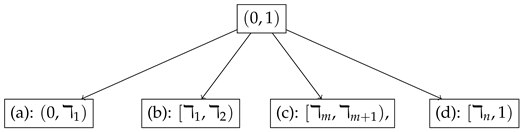
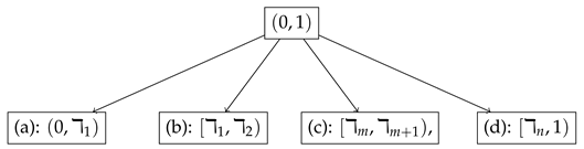
The required result is established for each mesh point ${\varkappa }_j\in (0,1)$ by partitioning the interval $(0,1)$, as shown in the figure below, for $2\le m\le n-1$. In each scenario, the local truncation error is first estimated. This is followed by the formulation of a suitable barrier function, designed to capture the essential properties of the solution within a specified domain. By utilizing these barrier functions, the desired estimate is obtained.

• Case (a):${\varkappa }_j\in (0,{\daleth }_1)$.

Clearly, ${\varkappa }_{j+1}-{\varkappa }_{j-1}\le C{ϵ}_1{\mu }^{-1}{N}^{-1}lnN$. Then, utilizing the standard approach to local truncation through Taylor expansions, error estimates are obtained, which are valid for ${\varkappa }_j\in (0,{\daleth }_1)$ and $1\le i\le n$, as follows:

$$\begin{array}{c}\hfill |{\left({\overrightarrow{L}}_1^N({\overrightarrow{W}}^{L_1}-{\overrightarrow{w}}^{L_1})\right)}_i\left({\varkappa }_j\right)|\le C{N}^{-1}{\mu }^{2}lnN\left({\displaystyle \sum _{k=1}^{i-1}{ϵ}_k^{-1}{\mathfrak{B}}_k^{l_1}\left({\varkappa }_{j-1}\right)+\sum _{k=i}^n{ϵ}_k^{-1}{\mathfrak{B}}_k^{l_1}\left({\varkappa }_{j-1}\right)}\right),\end{array}$$

(75)

$$\begin{array}{c}\hfill |{\left({\overrightarrow{L}}_2^N({\overrightarrow{W}}^{L_2}-{\overrightarrow{w}}^{L_2})\right)}_i\left({\varkappa }_j\right)|\le C{N}^{-1}{\mu }^{2}lnN\left({\displaystyle \sum _{k=1}^{i-1}{ϵ}_k^{-1}{\mathfrak{B}}_k^{l_2}\left({\varkappa }_{j-1}\right)+\sum _{k=i}^n{ϵ}_k^{-1}{\mathfrak{B}}_k^{l_2}\left({\varkappa }_{j-1}\right)}\right).\end{array}$$

(76)

Let the mesh functions be defined for ${\varkappa }_j\in (0,{\daleth }_1)$, where $1\le i\le n$ and $p=1,2$, as follows:

$${\varphi }_i\left({\varkappa }_j\right)=C{N}^{-1}lnN\left(\sum _{k=1}^{i-1}{e}^{{\displaystyle \frac{2\nu \mu H_1}{{ϵ}_k}}}{\mathit{B}}_k^{(l_p,N)}\left({\varkappa }_j\right)+\sum _{k=i}^n{e}^{{\displaystyle \frac{2\nu \mu H_1}{{ϵ}_k}}}{\mathit{B}}_k^{(l_p,N)}\left({\varkappa }_j\right)\right)+\sum _{k=1}^n{\mathit{B}}_k^{(l_p,N)}\left({\daleth }_k\right).$$

Utilizing the minimum principle and barrier function ${\overrightarrow{\mathrm{\Psi }}}^{\pm }\left({\varkappa }_j\right)=\overrightarrow{\varphi }\left({\varkappa }_j\right)\pm ({\overrightarrow{W}}^{L_1}-{\overrightarrow{w}}^{L_1})\left({\varkappa }_j\right)$, it has been established that $|({\overrightarrow{W}}^{L_1}-{\overrightarrow{w}}^{L_1})\left({\varkappa }_j\right)|\le C{N}^{-1}lnN.$ Similarly, for the interval (1,2), we have $|({\overrightarrow{W}}^{L_2}-{\overrightarrow{w}}^{L_2})\left({\varkappa }_j\right)|\le C{N}^{-1}lnN.$

• Case (b):${\varkappa }_j\in [{\daleth }_1,{\daleth }_2)$.

The two scenarios considered are Case (b1): $d_1=0$ and Case (b2): $d_1>0$. Case (b1): In this case, where $d_1=0$, the mesh is uniform within the interval $(0,{\daleth }_2)$. Consequently, for any ${\varkappa }_{j+1}-{\varkappa }_{j-1}\le C{ϵ}_1{\mu }^{-1}{N}^{-1}lnN$, for ${\varkappa }_j\in [{\daleth }_1,{\daleth }_2)$. Then,

$$\begin{array}{c}\hfill |{\left({\overrightarrow{L}}_1^N({\overrightarrow{W}}^{L_1}-{\overrightarrow{w}}^{L_1})\right)}_i\left({\varkappa }_j\right)|\le C{N}^{-1}{\mu }^{2}lnN\left({\displaystyle \sum _{k=1}^{i-1}{ϵ}_k^{-1}{\mathfrak{B}}_k^{l_1}\left({\varkappa }_{j-1}\right)+\sum _{k=i}^n{ϵ}_k^{-1}{\mathfrak{B}}_k^{l_1}\left({\varkappa }_{j-1}\right)}\right).\end{array}$$

(77)

Now, for ${\varkappa }_j\in [{\daleth }_1,{\daleth }_2)$ and $1\le i\le n$, define

$${\varphi }_i\left(x_j\right)=C{N}^{-1}lnN\left(\sum _{k=1}^{i-1}{e}^{{\displaystyle \frac{2\nu \mu H_2}{{ϵ}_k}}}{\mathit{B}}_k^{(l_p,N)}\left({\varkappa }_j\right)+\sum _{k=i}^n{e}^{{\displaystyle \frac{2\nu \mu H_2}{{ϵ}_k}}}{\mathit{B}}_k^{(l_p,N)}\left({\varkappa }_j\right)\right)+\sum _{k=2}^n{\mathit{B}}_k^{(l_p,N)}\left({\daleth }_k\right).$$

Utilizing the minimum principle and barrier function ${\overrightarrow{\mathrm{\Psi }}}^{\pm }\left({\varkappa }_j\right)=\overrightarrow{\varphi }\left({\varkappa }_j\right)\pm ({\overrightarrow{W}}^{L_1}-{\overrightarrow{w}}^{L_1})\left({\varkappa }_j\right)$, it has been derived that $|({\overrightarrow{W}}^{L_1}-{\overrightarrow{w}}^{L_1})\left({\varkappa }_j\right)|\le C{N}^{-1}lnN.$ Similarly, for the interval (1,2), we have $|({\overrightarrow{W}}^{L_2}-{\overrightarrow{w}}^{L_2})\left({\varkappa }_j\right)|\le C{N}^{-1}lnN.$ Case (b2): In this case, where $d_1>0$, ${\varkappa }_{j+1}-{\varkappa }_{j-1}\le C{ϵ}_2{N}^{-1}{\mu }^{-1}lnN$. Hence, for ${\varkappa }_j\in [{\daleth }_1,{\daleth }_2)$, by utilizing the standard approach to local truncation errors in Taylor series expansions, $\overline{h}={\varkappa }_{j+1}-{\varkappa }_{j-1}$. Then,

$$\begin{array}{c}\hfill |{\left({\overrightarrow{L}}_1^N({\overrightarrow{W}}^{L_1}-{\overrightarrow{w}}^{L_1})\right)}_i\left({\varkappa }_j\right)|\le C{ϵ}_i\mu |w_{i,1}^{L_1,\left(2\right)}\left({\varkappa }_{j-1}\right)|+C({\varkappa }_{j+1}-{\varkappa }_{j-1}){ϵ}_i\sum _{k=2}^n|w_{i,k}^{L_1,\left(3\right)}\left({\varkappa }_{j-1}\right)|\\ \hfill +C\mu |w_{i,1}^{L_1,\left(1\right)}\left({\varkappa }_{j-1}\right)|+C({\varkappa }_{j+1}-{\varkappa }_{j-1})\sum _{k=2}^n|w_{i,k}^{L_1,\left(2\right)}\left({\varkappa }_{j-1}\right)|.\end{array}$$

Now, using Lemma 3, it is not hard to derive that

$$|{\left({\overrightarrow{L}}_1^N({\overrightarrow{W}}^{L_1}-{\overrightarrow{w}}^{L_1})\right)}_1\left({\varkappa }_j\right)|\le C{N}^{-1}lnN{\mu }^2\sum _{k=2}^n{ϵ}_k^{-1}{\mathfrak{B}}_k^{l_1}\left({\varkappa }_{j-1}\right)+C{\mu }^2{ϵ}_1^{-1}{\mathfrak{B}}_1^{l_1}\left({\varkappa }_{j-1}\right),$$

and, for $2\le i\le n$, we have

$$|{\left({\overrightarrow{L}}_1^N({\overrightarrow{W}}^{L_1}-{\overrightarrow{w}}^{L_1})\right)}_i\left({\varkappa }_j\right)|\le C{N}^{-1}lnN{\mu }^2\sum _{k=i}^n{ϵ}_k^{-1}{\mathfrak{B}}_k^{l_1}\left({\varkappa }_{j-1}\right)+C{\mu }^2{ϵ}_i^{-1}{\mathfrak{B}}_1^{l_1}\left({\varkappa }_{j-1}\right).$$

Specify

$${\varphi }_1\left(x_j\right)=C{N}^{-1}lnN\sum _{k=2}^{n}exp(2\alpha \mu H_2/{ϵ}_k){\mathit{B}}_k^{(l_p,N)}\left(x_j\right)+C{\mathit{B}}_1^{(l_p,N)}\left(x_j\right)+\sum _{k=2}^n{\mathit{B}}_k^{(l_p,N)}\left({\daleth }_k\right)$$

and, for $2\le i\le n$, we have

$${\varphi }_i\left(x_j\right)=C{N}^{-1}lnN\sum _{k=i}^{n}exp(2\alpha \mu H_2/{ϵ}_k){\mathit{B}}_k^{(l_p,N)}\left(x_j\right)+C{\mathit{B}}_1^{(l_p,N)}\left(x_j\right)+\sum _{k=2}^n{\mathit{B}}_k^{(l_p,N)}\left({\daleth }_k\right).$$

• Case (c): ${\varkappa }_j\in [{\daleth }_m,{\daleth }_{m+1})$.

The three scenarios are outlined below. Case (c1): $d_1=d_2=\cdots =d_m=0$, Case (c2): $d_q>0$ and $d_{q+1}=\cdots =d_m=0$ for some q, $1\le q\le m-1$, Case (c3): $d_m>0$. Case (c1): $d_1=d_2=\cdots =d_m=0$. Since ${\daleth }_1=C{\daleth }_{m+1}$ and the mesh remains uniform over the interval $(0,{\daleth }_{m+1})$, it can be concluded that for ${\varkappa }_j\in ({\daleth }_m,{\daleth }_{m+1}]$, ${\varkappa }_{j+1}-{\varkappa }_{j-1}\le C{ϵ}_1{\mu }^{-1}{N}^{-1}lnN.$ Hence,

$$|{\left({\overrightarrow{L}}_1^N({\overrightarrow{W}}^{L_1}-{\overrightarrow{w}}^{L_1})\right)}_i\left({\varkappa }_j\right)|\le C{N}^{-1}{\mu }^{2}lnN\left({\displaystyle \sum _{k=1}^{i-1}{ϵ}_k^{-1}{\mathfrak{B}}_k^{l_1}\left({\varkappa }_{j-1}\right)+\sum _{k=i}^n{ϵ}_k^{-1}{\mathfrak{B}}_k^{l_1}\left({\varkappa }_{j-1}\right)}\right),$$

$$|{\left({\overrightarrow{L}}_2^N({\overrightarrow{W}}^{L_2}-{\overrightarrow{w}}^{L_2})\right)}_i\left({\varkappa }_j\right)|\le C{N}^{-1}{\mu }^{2}lnN\left({\displaystyle \sum _{k=1}^{i-1}{ϵ}_k^{-1}{\mathfrak{B}}_k^{l_2}\left({\varkappa }_{j-1}\right)+\sum _{k=i}^n{ϵ}_k^{-1}{\mathfrak{B}}_k^{l_2}\left({\varkappa }_{j-1}\right)}\right).$$

For $1\le i\le n$,

$${\varphi }_i\left({\varkappa }_j\right)=C{N}^{-1}lnN\left(\sum _{k=1}^{i-1}{e}^{{\displaystyle \frac{2\nu \mu H_{m+1}}{{ϵ}_k}}}{\mathit{B}}_k^{(l_p,N)}\left({\varkappa }_j\right)+\sum _{k=i}^n{e}^{{\displaystyle \frac{2\nu \mu H_{m+1}}{{ϵ}_k}}}{\mathit{B}}_k^{(l_p,N)}\left({\varkappa }_j\right)\right)+\sum _{k=m+1}^n{\mathit{B}}_k^{(l_p,N)}\left({\daleth }_k\right).$$

Utilizing the minimum principle and barrier function ${\overrightarrow{\mathrm{\Psi }}}^{\pm }\left({\varkappa }_j\right)=\overrightarrow{\varphi }\left({\varkappa }_j\right)\pm ({\overrightarrow{W}}^{L_1}-{\overrightarrow{w}}^{L_1})\left({\varkappa }_j\right)$, it has been derived that $|({\overrightarrow{W}}^{L_1}-{\overrightarrow{w}}^{L_1})\left({\varkappa }_j\right)|\le C{N}^{-1}lnN.$ Similarly, for the interval (1,2), we have $|({\overrightarrow{W}}^{L_2}-{\overrightarrow{w}}^{L_2})\left({\varkappa }_j\right)|\le C{N}^{-1}lnN.$ Case (c2): $d_q>0$ and $d_{q+1}=\cdots =d_m=0$ for some q, $1\le q\le m-1$. In this case, since ${\daleth }_{q+1}=C{\daleth }_{m+1}$, the region $({\daleth }_q,{\daleth }_{m+1})$ exhibits uniform mesh points and satisfies ${\varkappa }_{j+1}-{\varkappa }_{j-1}\le C{ϵ}_{q+1}{N}^{-1}{\mu }^{-1}lnN$, for any point ${\varkappa }_j\in ({\daleth }_m,{\daleth }_{m+1}]$. The utilized approach to local truncation is derived from Taylor expansions, as follows:

$$\begin{array}{c}\hfill |{\left({\overrightarrow{L}}_1^N({\overrightarrow{W}}^{L_1}-{\overrightarrow{w}}^{L_1})\right)}_i\left({\varkappa }_j\right)|\le C{ϵ}_i\mu \sum _{k=1}^q|w_{i,k}^{L_1,\left(2\right)}\left({\varkappa }_{j-1}\right)|+C({\varkappa }_{j+1}-{\varkappa }_{j-1}){ϵ}_i\sum _{k=q+1}^n|w_{i,k}^{L_1,\left(3\right)}\left({\varkappa }_{j-1}\right)|\\ \hfill +C\mu \sum _{k=1}^q|w_{i,k}^{L_1,\left(1\right)}\left({\varkappa }_{j-1}\right)|+C({\varkappa }_{j+1}-{\varkappa }_{j-1})\sum _{k=q+1}^n|w_{i,k}^{L_1,\left(2\right)}\left({\varkappa }_{j-1}\right)|.\end{array}$$

Now, utilizing Lemma 3, it is evident that for $i\le q$, we have

$$|{\left({\overrightarrow{L}}_1^N({\overrightarrow{W}}^{L_1}-{\overrightarrow{w}}^{L_1})\right)}_i\left({\varkappa }_j\right)|\le C{N}^{-1}{\mu }^{2}lnN\sum _{k=q+1}^n{ϵ}_k^{-1}{\mathfrak{B}}_k^{l_1}\left({\varkappa }_{j-1}\right)+C\sum _{k=i}^q{ϵ}_k^{-1}{\mathfrak{B}}_k^{l_1}\left({\varkappa }_{j-1}\right)$$

and, for $i>q$, we have

$$|{\left({\overrightarrow{L}}_1^N({\overrightarrow{W}}^{L_1}-{\overrightarrow{w}}^{L_1})\right)}_i\left({\varkappa }_j\right)|\le C{\displaystyle \frac{1}{N}}{\mu }^{2}lnN\sum _{k=i}^n{ϵ}_k^{-1}{\mathfrak{B}}_k^{l_1}\left({\varkappa }_{j-1}\right)+C{ϵ}_i^{-1}{\mathfrak{B}}_q^{l_1}\left({\varkappa }_{j-1}\right).$$

Now, for $i\le q$, specify

$${\varphi }_i\left({\varkappa }_j\right)=C{\displaystyle \frac{1}{N}}lnN\sum _{k=q+1}^{n}exp\left({\displaystyle \frac{2\alpha \mu H_{m+1}}{{ϵ}_k}}\right){\mathit{B}}_k^{(l_p,N)}\left({\varkappa }_j\right)+C\sum _{k=i}^q{\mathit{B}}_k^{(l_p,N)}\left({\varkappa }_j\right)+C\sum _{k=m+1}^n{\mathit{B}}_k^{(l_p,N)}\left({\daleth }_k\right)$$

and, for $i>q$, specify

$${\varphi }_i\left({\varkappa }_j\right)=C{\displaystyle \frac{1}{N}}lnN\sum _{k=i}^{n}exp\left({\displaystyle \frac{2\alpha \mu H_{m+1}}{{ϵ}_k}}\right){\mathit{B}}_k^{(l_p,N)}\left({\varkappa }_j\right)+C{\mathit{B}}_q^{(l_p,N)}\left({\varkappa }_j\right)+C\sum _{k=m+1}^n{\mathit{B}}_k^{(l_p,N)}\left({\daleth }_k\right).$$

• Case (c3):$d_m>0$. In the previous arguments of Case (c2), by replacing q with m and applying the inequality $x_{j+1}-x_{j-1}\le C{\displaystyle \frac{{ϵ}_{m+1}}{N}}{\mu }^{-1}lnN$, the estimates are valid for ${\varkappa }_j\in ({\daleth }_m,{\daleth }_{m+1}]$.For $i\le m$, we have

  $$|{\left({\overrightarrow{L}}_1^N({\overrightarrow{W}}^{L_1}-{\overrightarrow{w}}^{L_1})\right)}_i\left({\varkappa }_j\right)|\le C{N}^{-1}{\mu }^{2}lnN\sum _{k=m+1}^n{ϵ}_k^{-1}{\mathfrak{B}}_k^{l_1}\left({\varkappa }_{j-1}\right)+C\sum _{k=i}^m{ϵ}_k^{-1}{\mathfrak{B}}_k^{l_1}\left({\varkappa }_{j-1}\right)$$

  and, for $i>m$, we have

  $$|{\left({\overrightarrow{L}}_1^N({\overrightarrow{W}}^{L_1}-{\overrightarrow{w}}^{L_1})\right)}_i\left({\varkappa }_j\right)|\le C{\displaystyle \frac{1}{N}}{\mu }^{2}lnN\sum _{k=i}^n{ϵ}_k^{-1}{\mathfrak{B}}_k^{l_1}\left({\varkappa }_{j-1}\right)+C{ϵ}_i^{-1}{\mathfrak{B}}_m^{l_1}\left({\varkappa }_{j-1}\right).$$

  For $i\le m$, define

  $${\varphi }_i\left({\varkappa }_j\right)=C{\displaystyle \frac{1}{N}}lnN\sum _{k=m+1}^{n}exp\left({\displaystyle \frac{2\alpha \mu H_{m+1}}{{ϵ}_k}}\right){\mathit{B}}_k^{(l_p,N)}\left({\varkappa }_j\right)+C\sum _{k=i}^m{\mathit{B}}_k^{(l_p,N)}\left({\varkappa }_j\right)+C\sum _{k=m+1}^n{\mathit{B}}_k^{(l_p,N)}\left({\daleth }_k\right)$$

  and, for $i>m$, define

  $${\varphi }_i\left({\varkappa }_j\right)=C{\displaystyle \frac{1}{N}}lnN\sum _{k=i}^{n}exp\left({\displaystyle \frac{2\alpha \mu H_{m+1}}{{ϵ}_k}}\right){\mathit{B}}_k^{(l_p,N)}\left({\varkappa }_j\right)+C{\mathit{B}}_m^{(l_p,N)}\left({\varkappa }_j\right)+C\sum _{k=m+1}^n{\mathit{B}}_k^{(l_p,N)}\left({\daleth }_k\right).$$

• Case (d):

There are three distinct cases that need to be considered: Case (d1): $d_1=\cdots =d_n=0$, Case (d2): $d_q>0$ and $d_{q+1}=\cdots =d_n=0$ for some q, $1\le q\le n-1$ and Case (d3): $d_n>0$. Case (d1): $d_1=\cdots =d_n=0$. In this case, the mesh is uniformly distributed over the interval $[0,1]$. The corresponding result for this situation is derived in Lemma 9. Case (d2): $d_q>0$ and $d_{q+1}=\cdots =d_n=0$ for some q, $1\le q\le n-1$. For this scenario, based on the definition of ${\daleth }_n$, it can be shown that ${\varkappa }_{j+1}-{\varkappa }_{j-1}\le C{ϵ}_{q+1}{N}^{-1}{\mu }^{-1}lnN.$ Moreover, by applying analogous arguments similar to Case (c2), this leads to the estimates for ${\varkappa }_j\in ({\daleth }_n,1]$. For $i\le q$,

$$|{\left({\overrightarrow{L}}_1^N({\overrightarrow{W}}^{L_1}-{\overrightarrow{w}}^{L_1})\right)}_i\left({\varkappa }_j\right)|\le C{N}^{-1}{\mu }^{2}lnN\sum _{k=q+1}^n{ϵ}_k^{-1}{\mathfrak{B}}_k^{l_1}\left({\varkappa }_{j-1}\right)+C\sum _{k=i}^q{ϵ}_k^{-1}{\mathfrak{B}}_k^{l_1}\left({\varkappa }_{j-1}\right)$$

and, for $i>q$,

$$|{\left({\overrightarrow{L}}_1^N({\overrightarrow{W}}^{L_1}-{\overrightarrow{w}}^{L_1})\right)}_i\left({\varkappa }_j\right)|\le C{\displaystyle \frac{1}{N}}{\mu }^{2}lnN\sum _{k=i}^n{ϵ}_k^{-1}{\mathfrak{B}}_k^{l_1}\left({\varkappa }_{j-1}\right)+C{ϵ}_i^{-1}{\mathfrak{B}}_q^{l_1}\left({\varkappa }_{j-1}\right).$$

Now define, for $i\le q$, the following:

$${\varphi }_i\left({\varkappa }_j\right)=C{\displaystyle \frac{1}{N}}lnN\sum _{k=q+1}^{n}exp\left({\displaystyle \frac{2\alpha \mu H_{n+1}}{{ϵ}_k}}\right){\mathit{B}}_k^{(l_p,N)}\left({\varkappa }_j\right)+C\sum _{k=i}^q{\mathit{B}}_k^{(l_p,N)}\left({\varkappa }_j\right)$$

and, for $i>q$, define

$${\varphi }_i\left({\varkappa }_j\right)=C{\displaystyle \frac{1}{N}}lnN\sum _{k=i}^{n}exp\left({\displaystyle \frac{2\alpha \mu H_{n+1}}{{ϵ}_k}}\right){\mathit{B}}_k^{(l_p,N)}\left({\varkappa }_j\right)+C{\mathit{B}}_q^{(l_p,N)}\left({\varkappa }_j\right),$$

respectively. Case (d3): For $d_n>0$, let ${\daleth }_n$ be defined as ${\daleth }_n={\displaystyle \frac{{ϵ}_n}{\mu \alpha }}lnN$. Then, considering the interval $({\daleth }_n,1]$, we have

$$\begin{array}{cc}\hfill |({W_i}^{L_1}-{w_i}^{L_1})\left({\varkappa }_j\right)|& \le |{W_i}^{L_1}\left({\varkappa }_j\right)|+|{w_i}^{L_1}\left({\varkappa }_j\right)|\hfill \\ \hfill & \le C{\mathit{B}}_n^{(l_1,N)}\left({\varkappa }_j\right)+C{\mathfrak{B}}_n^{l_1}\left({\varkappa }_j\right)\hfill \\ \hfill & \le C{\mathit{B}}_n^{(l_1,N)}\left({\daleth }_n\right)+C{\mathfrak{B}}_n^{l_1}\left({\daleth }_n\right)\le C{N}^{-1}.\hfill \end{array}$$

Hence, $|({W_i}^{L_1}-{w_i}^{L_1})\left({\varkappa }_j\right)|\le C{N}^{-1},\mathrm{and}|({W_i}^{L_2}-{w_i}^{L_2})\left({\varkappa }_j\right)|\le C{N}^{-1}.$ Thus, for each of the cases, the barrier function is constructed. Moreover, using minimum principle, it was derived that $|({\overrightarrow{W}}^{L_1}-{\overrightarrow{w}}^{L_1})\left({\varkappa }_j\right)|\le C{N}^{-1}lnN\mathrm{and}|({\overrightarrow{W}}^{L_2}-{\overrightarrow{w}}^{L_2})\left({\varkappa }_j\right)|\le C{N}^{-1}lnN.$ Therefore,

$$|({\overrightarrow{W}}^L-{\overrightarrow{w}}^L)\left({\varkappa }_j\right)|\le C{N}^{-1}lnN.$$

The proof of the lemma is completed. □

The bounds on the error in the singular components ${\overrightarrow{w}}^{L_1}$ and ${\overrightarrow{w}}^{L_2}$ are estimated for the case $\alpha {\mu }^2\ge \gamma {ϵ}_i$. These estimates are derived by utilizing the mesh functions ${\mathit{B}}_i^{(l_p,N)}\left({\varkappa }_j\right)$, where $1\le i\le n$, which are defined over ${\overline{\mathrm{\Omega }}}^N$ as follows:

$$\begin{array}{cc}\hfill {\mathit{B}}_i^{(l_p,N)}\left({\varkappa }_j\right)=& \prod _{k=1}^j{\left(1+\sqrt{{\displaystyle \frac{\gamma \alpha }{{ϵ}_i}}}{h}_k\right)}^{-1},\hfill \end{array}$$

(78)

with ${\mathit{B}}_i^{(l_p,N)}\left({\varkappa }_0\right)=1$, for ${\mathrm{\Omega }}_1,p=1$, for ${\mathrm{\Omega }}_2,p=2$.

Lemma 11.

Let ${\overrightarrow{w}}^{L_1}$ and ${\overrightarrow{w}}^{L_2}$ satisfy (13), and let ${\overrightarrow{W}}^{L_1}$ and ${\overrightarrow{W}}^{L_2}$ satisfy (67) and (68). Then,

$$\parallel {\overrightarrow{W}}^{L_1}-{\overrightarrow{w}}^{L_1}\parallel \le C{N}^{-1}lnN,\parallel {\overrightarrow{W}}^{L_2}-{\overrightarrow{w}}^{L_2}\parallel \le C{N}^{-1}lnN.$$

Proof. 

Assume that $d_q=0$. For $q=1,2,\cdots ,n$, the local truncation error is given by

$$|{\overrightarrow{L}}_1^N({\overrightarrow{W}}^{L_1}-{\overrightarrow{w}}^{L_1})\left({\varkappa }_j\right)|\le C({\varkappa }_{j+1}-{\varkappa }_{j-1})\left(\begin{array}{c}{ϵ}_i\parallel w_i^{L_1{,}^{\prime \prime \prime }}{\parallel }_D+\mu {\parallel w_i^{L_1{,}^{\prime \prime }}\parallel }_D\end{array}\right)$$

(79)

$$|{\overrightarrow{L}}_2^N({\overrightarrow{W}}^{L_2}-{\overrightarrow{w}}^{L_2})\left({\varkappa }_j\right)|\le C({\varkappa }_{j+1}-{\varkappa }_{j-1})\left(\begin{array}{c}{ϵ}_i\parallel w_i^{L_2{,}^{\prime \prime \prime }}{\parallel }_D+\mu {\parallel w_i^{L_2{,}^{\prime \prime }}\parallel }_D\end{array}\right)$$

(80)

where $D=[{\varkappa }_{j-1},{\varkappa }_{j+1}]$. Since $d_q=0$, the mesh ${\overline{\mathrm{\Omega }}}^N$ is uniform. Then, the value of $h=N^{-1}$. In this instance, ${ϵ}_k^{-1/2}\le ClnN$,

$$\begin{array}{c}\hfill |{\left({\overrightarrow{L}}_1^N({\overrightarrow{W}}^{L_1}-{\overrightarrow{w}}^{L_1})\right)}_i\left({\varkappa }_j\right)|\le C({\varkappa }_{j+1}-{\varkappa }_{j-1})\left({\displaystyle \sum _{k=1}^{i-1}{ϵ}_k^{-1/2}{\mathfrak{B}}_k^{l_1}\left({\varkappa }_{j-1}\right)+\sum _{k=i}^n{ϵ}_k^{-1/2}{\mathfrak{B}}_k^{l_1}\left({\varkappa }_{j-1}\right)}\right)\le C{N}^{-1}lnN.\end{array}$$

This is established for each mesh point ${\varkappa }_j\in (0,1)$ by partitioning the interval $(0,1)$ as follows, for $2\le m\le n-1$: In each scenario, the local truncation error is first estimated. This is followed by the formulation of a suitable barrier function, designed to capture the essential properties of the solution within a specified domain. By utilizing these barrier functions, the desired estimate is obtained.

• Case (a):${\varkappa }_j\in (0,{\daleth }_1)$.

Clearly, ${\varkappa }_{j+1}-{\varkappa }_{j-1}\le C\sqrt{{ϵ}_1}{N}^{-1}lnN$. Then, by utilizing the approach to local truncation in Taylor expansions, error estimates are obtained, which are valid for ${\varkappa }_j\in (0,{\daleth }_1)$ and $1\le i\le n$, as follows:

$$\begin{array}{c}\hfill |{\left({\overrightarrow{L}}_1^N({\overrightarrow{W}}^{L_1}-{\overrightarrow{w}}^{L_1})\right)}_i\left({\varkappa }_j\right)|\le C{N}^{-1}\sqrt{{ϵ}_1}lnN\left({\displaystyle \sum _{k=1}^{i-1}{ϵ}_k^{-1/2}{\mathfrak{B}}_k^{l_1}\left({\varkappa }_{j-1}\right)+\sum _{k=i}^n{ϵ}_k^{-1/2}{\mathfrak{B}}_k^{l_1}\left({\varkappa }_{j-1}\right)}\right)\le C{N}^{-1}lnN,\end{array}$$

$$\begin{array}{c}\hfill |{\left({\overrightarrow{L}}_2^N({\overrightarrow{W}}^{L_2}-{\overrightarrow{w}}^{L_2})\right)}_i\left({\varkappa }_j\right)|\le C{N}^{-1}\sqrt{{ϵ}_1}lnN\left({\displaystyle \sum _{k=1}^{i-1}{ϵ}_k^{-1/2}{\mathfrak{B}}_k^{l_2}\left({\varkappa }_{j-1}\right)+\sum _{k=i}^n{ϵ}_k^{-1/2}{\mathfrak{B}}_k^{l_2}\left({\varkappa }_{j-1}\right)}\right)\le C{N}^{-1}lnN.\end{array}$$

• Case (b):  ${\varkappa }_j\in [{\daleth }_1,{\daleth }_2)$

The two scenarios considered are Case (b1): $d_1=0$ and Case (b2): $d_1>0$. Case (b1): $d_1=0$. In this case, the mesh is uniform within the interval $(0,{\daleth }_2)$. Consequently, for any ${\varkappa }_{j+1}-{\varkappa }_{j-1}\le C\sqrt{{ϵ}_1}{N}^{-1}lnN$, for ${\varkappa }_j\in [{\daleth }_1,{\daleth }_2)$. Then,

$$\begin{array}{c}\hfill |{\left({\overrightarrow{L}}_1^N({\overrightarrow{W}}^{L_1}-{\overrightarrow{w}}^{L_1})\right)}_i\left({\varkappa }_j\right)|\le C{N}^{-1}\sqrt{{ϵ}_1}lnN\left({\displaystyle \sum _{k=1}^{i-1}{ϵ}_k^{-1/2}{\mathfrak{B}}_k^{l_1}\left({\varkappa }_{j-1}\right)+\sum _{k=i}^n{ϵ}_k^{-1/2}{\mathfrak{B}}_k^{l_1}\left({\varkappa }_{j-1}\right)}\right)\le C{N}^{-1}lnN.\end{array}$$

• Case (b2): $d_1>0$. Tor this case, ${\varkappa }_{j+1}-{\varkappa }_{j-1}\le C\sqrt{{ϵ}_2}{N}^{-1}{\mu }^{-1}lnN$. Hence, for ${\varkappa }_j\in [{\daleth }_1,{\daleth }_2)$, by utilizing the standard approach to local truncation errors in Taylor series expansions, the term $\overline{h}={\varkappa }_{j+1}-{\varkappa }_{j-1}$. Then, using Lemma 4, we have

  $$\begin{array}{c}\hfill |{\left({\overrightarrow{L}}_1^N({\overrightarrow{W}}^{L_1}-{\overrightarrow{w}}^{L_1})\right)}_i\left({\varkappa }_j\right)|\le C{N}^{-1}lnN.\end{array}$$

• Case (c): $x_j\in [{\daleth }_m,{\daleth }_{m+1})$.

The three scenarios are outlined below. Case (c1): $d_1=d_2=\cdots =d_m=0$, Case (c2): $d_q>0$ and $d_{q+1}=\cdots =d_m=0$ for some q, $1\le q\le m-1$ and Case (c3): $d_m>0$. Case (c1): $d_1=d_2=\cdots =d_m=0$. Since ${\daleth }_1=C{\daleth }_{m+1}$ and the mesh remains uniform over the interval $(0,{\daleth }_{m+1})$, it can be concluded that for ${\varkappa }_j\in ({\daleth }_m,{\daleth }_{m+1}]$, ${\varkappa }_{j+1}-{\varkappa }_{j-1}\le C\sqrt{{ϵ}_1}{N}^{-1}lnN.$ Hence,

$$\begin{array}{c}\hfill |{\left({\overrightarrow{L}}_1^N({\overrightarrow{W}}^{L_1}-{\overrightarrow{w}}^{L_1})\right)}_i\left({\varkappa }_j\right)|\le C{N}^{-1}\sqrt{{ϵ}_1}lnN\left({\displaystyle \sum _{k=1}^{i-1}{ϵ}_k^{-1/2}{\mathfrak{B}}_k^{l_1}\left({\varkappa }_{j-1}\right)+\sum _{k=i}^n{ϵ}_k^{-1/2}{\mathfrak{B}}_k^{l_1}\left({\varkappa }_{j-1}\right)}\right)\le C{N}^{-1}lnN.\end{array}$$

• Case (c2): $d_q>0$ and $d_{q+1}=\cdots =d_m=0$ for some q, $1\le q\le m-1$. Since ${\daleth }_{q+1}=C{\daleth }_{m+1}$, the mesh is uniform in $({\daleth }_q,{\daleth }_{m+1})$, which implies that ${\varkappa }_{j+1}-{\varkappa }_{j-1}\le C\sqrt{{ϵ}_{q+1}}{N}^{-1}lnN$, for ${\varkappa }_j\in ({\daleth }_m,{\daleth }_{m+1}]$. The approach to local truncation is derived from Taylor expansions, and it is outlined in Lemma 4, as follows:

  $$\begin{array}{c}\hfill |{\left({\overrightarrow{L}}_1^N({\overrightarrow{W}}^{L_1}-{\overrightarrow{w}}^{L_1})\right)}_i\left({\varkappa }_j\right)|\le C{N}^{-1}lnN.\end{array}$$

• Case (c3): $d_m>0$. In the previous arguments of Case (c2), by replacing q with m and applying the inequality ${\varkappa }_{j+1}-{\varkappa }_{j-1}\le C\sqrt{{ϵ}_{m+1}}{N}^{-1}{\mu }^{-1}lnN$, the estimates are valid for ${\varkappa }_j\in ({\daleth }_m,{\daleth }_{m+1}]$.

  $$\begin{array}{c}\hfill |{\left({\overrightarrow{L}}_1^N({\overrightarrow{W}}^{L_1}-{\overrightarrow{w}}^{L_1})\right)}_i\left({\varkappa }_j\right)|\le C{N}^{-1}\sqrt{{ϵ}_{m+1}}lnN\left({\displaystyle \sum _{k=1}^{i-1}{ϵ}_k^{-1/2}{\mathfrak{B}}_k^{l_1}\left({\varkappa }_{j-1}\right)+\sum _{k=i}^n{ϵ}_k^{-1/2}{\mathfrak{B}}_k^{l_1}\left({\varkappa }_{j-1}\right)}\right)\le C{N}^{-1}lnN.\end{array}$$

• Case (d): There are three distinct cases that need to be considered: Case (d1): $d_1=\cdots =d_n=0$, Case (d2): $d_q>0$ and $d_{q+1}=\cdots =d_n=0$ for some q, $1\le q\le n-1$ and Case (d3): $d_n>0$. Case (d1): $d_1=\cdots =d_n=0$. In this case, the mesh is uniformly distributed over the interval $[0,1]$. The corresponding result for this situation is derived in Lemma 9. Case (d2): $d_q>0$ and $d_{q+1}=\cdots =d_n=0$ for some q, $1\le q\le n-1$. For this scenario, based on the definition of ${\daleth }_n$, it can be shown that ${\varkappa }_{j+1}-{\varkappa }_{j-1}\le C\sqrt{{ϵ}_{q+1}}{N}^{-1}lnN.$ Moreover, by employing arguments analogous to Case (c2), this leads to the estimates for $x_j\in ({\daleth }_n,1]$. Case (d3): $d_n>0$. Let ${\daleth }_n$ be defined as ${\daleth }_n={\displaystyle \frac{{ϵ}_n}{\mu \alpha }}lnN$ on the interval $({\daleth }_n,1]$. Hence, $|({\overrightarrow{W}}^{L_1}-{\overrightarrow{w}}^{L_1})\left({\varkappa }_j\right)|\le C{N}^{-1}lnN$. Similarly,$|({\overrightarrow{W}}^{L_2}-{\overrightarrow{w}}^{L_2})\left({\varkappa }_j\right)|\le C{N}^{-1}lnN$. Therefore,

  $$|({\overrightarrow{W}}^L-{\overrightarrow{w}}^L)\left({\varkappa }_j\right)|\le C{N}^{-1}lnN.$$

  The proof of the lemma is completed. □

To establish the bounds on the error $|({\overrightarrow{W}}^{R_1}-{\overrightarrow{w}}^{R_1})\left({\varkappa }_j\right)|$, the mesh function is defined over ${\overline{\mathrm{\Omega }}}^N$

$$\begin{array}{c}\hfill {\mathit{B}}^{(r_p,N)}\left({\varkappa }_j\right)=\prod _{i=j+1}^N{\left(1+{\displaystyle \frac{\gamma h_i}{2\mu }}\right)}^{-1},{\mathit{B}}^{(r_p,N)}\left({\varkappa }_N\right)=1,\mathrm{where}{\mathit{B}}^{(r_p,N)},p=1,2.\end{array}$$

Lemma 12.

For the case $\alpha {\mu }^2\ge \gamma {ϵ}_j$, the layer components ${W_i}^{R_1}$ and ${W_i}^{R_2}$, $1\le i\le n$ satisfy the following bounds on ${\overline{\mathrm{\Omega }}}^N$:

$$|W_i^{R_1}\left({\varkappa }_j\right)|\le C{\mathit{B}}_n^{(r_1,N)}\left({\varkappa }_j\right),|W_i^{R_2}\left({\varkappa }_j\right)|\le C{\mathit{B}}_n^{(r_2,N)}\left({\varkappa }_j\right).$$

Proof. 

This result can be demonstrated by defining the mesh functions ${\overrightarrow{\mathrm{\Psi }}}^{R_1}\left({\varkappa }_j\right)=C{\mathit{B}}^{(r_1,N)}\left({\varkappa }_j\right)\pm {\overrightarrow{W}}^{R_1}$ and ${\overrightarrow{\mathrm{\Psi }}}^{R_2}\left({\varkappa }_j\right)=C{\mathit{B}}^{(r_2,N)}\left({\varkappa }_j\right)\pm {\overrightarrow{W}}^{R_2}$. Also, since ${\overrightarrow{W}}^{R_1}\left(0\right)\le e^{-{\displaystyle \frac{\gamma }{\mu }}}$, ${\overrightarrow{W}}^{R_1}\left(0\right)\le {\mathit{B}}^{(r_1,N)}\left({\varkappa }_0\right)$. Hence, ${\overrightarrow{\mathrm{\Psi }}}^{R_1}\left(0\right)\ge \overrightarrow{0}$. Also, for an appropriate choice of C, it follows that ${\overrightarrow{\mathrm{\Psi }}}^{R_1}\left({\varkappa }_N\right)\ge \overrightarrow{0}$. Further, ${\overrightarrow{L}}_1^N{\overrightarrow{\mathrm{\Psi }}}^{R_1}\left({\varkappa }_j\right)\le \overrightarrow{0}$ and ${\overrightarrow{L}}_2^N{\overrightarrow{\mathrm{\Psi }}}^{R_2}\left({\varkappa }_j\right)\le \overrightarrow{0}$. Hence, by the minimum principle, ${\overrightarrow{\mathrm{\Psi }}}^{R_1}\left({\varkappa }_j\right)\ge \overrightarrow{0}$ and ${\overrightarrow{\mathrm{\Psi }}}^{R_2}\left({\varkappa }_j\right)\ge \overrightarrow{0}$, for $0\le j\le N$. Hence, $|{\overrightarrow{W}}^{R_1}\left({\varkappa }_j\right)|\le C{\mathit{B}}^{(r_1,N)}\left({\varkappa }_j\right)\mathrm{and}|{\overrightarrow{W}}^{R_2}\left({\varkappa }_j\right)|\le C{\mathit{B}}^{(r_2,N)}\left({\varkappa }_j\right)\mathrm{on}{\overline{\mathrm{\Omega }}}^N.$ The proof of the lemma is completed. □

Lemma 13.

At each point ${\varkappa }_j\in {\overline{\mathrm{\Omega }}}^N$, $|({\overrightarrow{W}}^R-{\overrightarrow{w}}^R)\left({\varkappa }_j\right)|\le C{N}^{-1}lnN$, for the case $\alpha {\mu }^2\ge \gamma {ϵ}_j$.

Proof. 

The local truncation error is given by

$$|{\overrightarrow{L}}_1^N({\overrightarrow{W}}^{R_1}-{\overrightarrow{w}}^{R_1})\left({\varkappa }_j\right)|\le C({\varkappa }_{j+1}-{\varkappa }_{j-1})\left(\begin{array}{c}{ϵ}_i\parallel w_i^{R_1{,}^{\prime \prime \prime }}{\parallel }_D+\mu {\parallel w_i^{R_1{,}^{\prime \prime }}\parallel }_D\end{array}\right)$$

(81)

where $D=[{\varkappa }_{j-1},{\varkappa }_{j+1}],{\mu }^{-1}\le ClnN$. Consider the case $d_1=0$. Then, ${\varkappa }_{j+1}-{\varkappa }_{j-1}\le C\mu N^{-1}lnN$. Hence, $|{\overrightarrow{L}}_1^N({\overrightarrow{W}}^{R_1}-{\overrightarrow{w}}^{R_1})\left({\varkappa }_j\right)|\le C{N}^{-1}lnN,$ $|{\overrightarrow{L}}_2^N({\overrightarrow{W}}^{R_2}-{\overrightarrow{w}}^{R_2})\left({\varkappa }_j\right)|\le C{N}^{-1}lnN.$ Consider the case $d_1>0,{\varkappa }_j\in (0,1-{\sigma }_1]$. Hence,

$$\begin{array}{cc}\hfill |{({\overrightarrow{W}}^{R_1}-{\overrightarrow{w}}^{R_1})}_i\left({\varkappa }_j\right)|& \le |{W_i}^{R_1}\left({\varkappa }_j\right)|+|{w_i}^{R_1}\left({\varkappa }_j\right)|\le C{\mathit{B}}^{(r_1,N)}\left({\varkappa }_j\right)+C{\mathfrak{B}}_i^{r_1}\left({\varkappa }_j\right)\hfill \\ \hfill & \le C{\mathit{B}}^{(r_1,N)}\left({\sigma }_1\right)+C{\mathfrak{B}}_i^{r_1}\left({\sigma }_1\right)\le C{N}^{-1},\hfill \end{array}$$

for ${\varkappa }_j\in (1,2-{\sigma }_1]$. Similarly, like above,

$$|{({\overrightarrow{W}}^{R_2}-{\overrightarrow{w}}^{R_2})}_i\left({\varkappa }_j\right)|\le |{W_i}^{R_2}\left({\varkappa }_j\right)|+|{w_i}^{R_2}\left({\varkappa }_j\right)|\le C{\mathit{B}}^{(r_2,N)}\left({\sigma }_1\right)+C{\mathfrak{B}}_2^{r_2}\left({\sigma }_1\right)\le C{N}^{-1}.$$

Examine the mesh region $(1-{\sigma }_1,1]$. It is known that $\overline{h}={\varkappa }_{j+1}-{\varkappa }_{j-1}$. Then, ${\varkappa }_{j+1}-{\varkappa }_{j-1}\le C\mu N^{-1}lnN$, $|{\overrightarrow{L}}_1^N({\overrightarrow{W}}^{R_1}-{\overrightarrow{w}}^{R_1})\left({\varkappa }_j\right)|\le C{N}^{-1}lnN.$ For $(2-{\sigma }_1,2]$, $|{\overrightarrow{L}}_2^N({\overrightarrow{W}}^{R_2}-{\overrightarrow{w}}^{R_2})\left({\varkappa }_j\right)|\le C{N}^{-1}lnN.$ The proof of the lemma is completed. □

Theorem 3.

Let $\overrightarrow{\mathfrak{u}}$ be the solution of (1) and let $\overrightarrow{\mathfrak{u}}$ be the solution of (62)–(64). Then, for each mesh point ${\varkappa }_j\in {\overline{\mathrm{\Omega }}}^N$,

$$\parallel \overrightarrow{\mathfrak{u}}-\overrightarrow{\mathfrak{u}}{\parallel }_{{\overline{\mathrm{\Omega }}}^N}\le C{N}^{-1}lnN,$$

for both of the cases $\alpha {\mu }^2\le \gamma {ϵ}_i$ and $\alpha {\mu }^2\ge \gamma {ϵ}_j$.

Proof. 

The proof follows Lemmas 7, 9, 11 and 13. □

12. Numerical Illustration

12.1. Example

The numerical approximation of the solution to the following system on the interval $(0,2)$ is obtained by applying the proposed method to both cases, where $\alpha {\mu }^2\le \gamma {ϵ}_i$ and $\alpha {\mu }^2\ge \gamma {ϵ}_j$, as follows:

$$E{\overrightarrow{\mathfrak{u}}}^{\prime \prime }\left(\varkappa \right)+\mu \mathcal{A}\left(\varkappa \right){\overrightarrow{\mathfrak{u}}}^{\prime }\left(\varkappa \right)-\mathcal{B}\left(\varkappa \right)\overrightarrow{\mathfrak{u}}\left(\varkappa \right)+\mathcal{D}\left(\varkappa \right)\overrightarrow{\mathfrak{u}}(\varkappa -1)=\overrightarrow{\mathit{f}}\left(\varkappa \right)\mathrm{for}\mathrm{all}\varkappa \in \mathrm{\Omega }=(0,2),$$

where $\mathcal{A}\left(\varkappa \right)=diag(0.5,0.5,0.5),\overrightarrow{\mathit{f}}\left(\varkappa \right)={(-1.0,-2.0,-1.5)}^T,\mathcal{B}\left(\varkappa \right)=\left(\begin{array}{ccc}6.0& -1.0& -1.0\\ -1.0& 6.0& -1.0\\ -1.0& -1.0& 6.0\end{array}\right),$ $\mathcal{D}\left(\varkappa \right)=diag(0.8,0.8,0.8)$.

12.2. Example

The numerical approximation of the solution to the following system on the interval $(0,2)$ is obtained by applying the proposed method to both cases, where $\alpha {\mu }^2\le \gamma {ϵ}_i$ and $\alpha {\mu }^2\ge \gamma {ϵ}_j$, as follows:

$$E{\overrightarrow{\mathfrak{u}}}^{\prime \prime }\left(\varkappa \right)+\mu \mathcal{A}\left(\varkappa \right){\overrightarrow{\mathfrak{u}}}^{\prime }\left(\varkappa \right)-\mathcal{B}\left(\varkappa \right)\overrightarrow{\mathfrak{u}}\left(\varkappa \right)+\mathcal{D}\left(\varkappa \right)\overrightarrow{\mathfrak{u}}(\varkappa -1)=\overrightarrow{\mathit{f}}\left(\varkappa \right)\mathrm{for}\mathrm{all}\varkappa \in \mathrm{\Omega }=(0,2),$$

where $\mathcal{A}\left(\varkappa \right)=diag(0.3,0.5,0.7),\overrightarrow{\mathit{f}}\left(\varkappa \right)={(-2.0,-1.5,-2.0)}^T,\mathcal{B}\left(\varkappa \right)=\left(\begin{array}{ccc}7.0& -1.0& -1.0\\ -1.5& 8.0& -1.0\\ -2.0& -1.0& 6.0\end{array}\right),$ $\mathcal{D}\left(\varkappa \right)=diag(1.0,1.0,1.0)$.

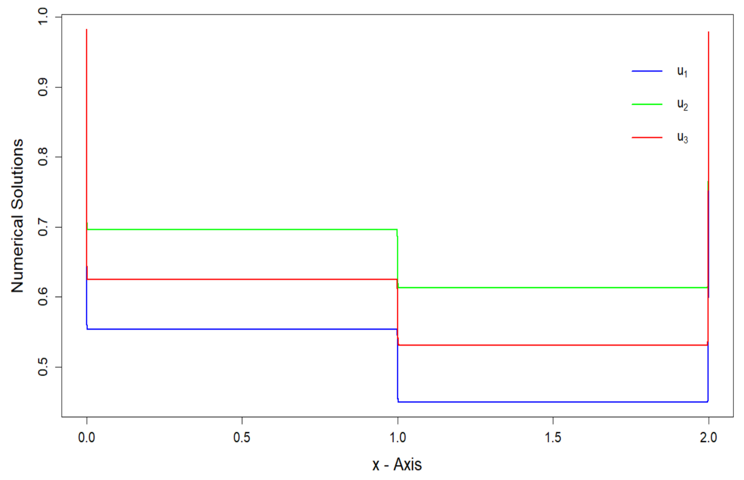
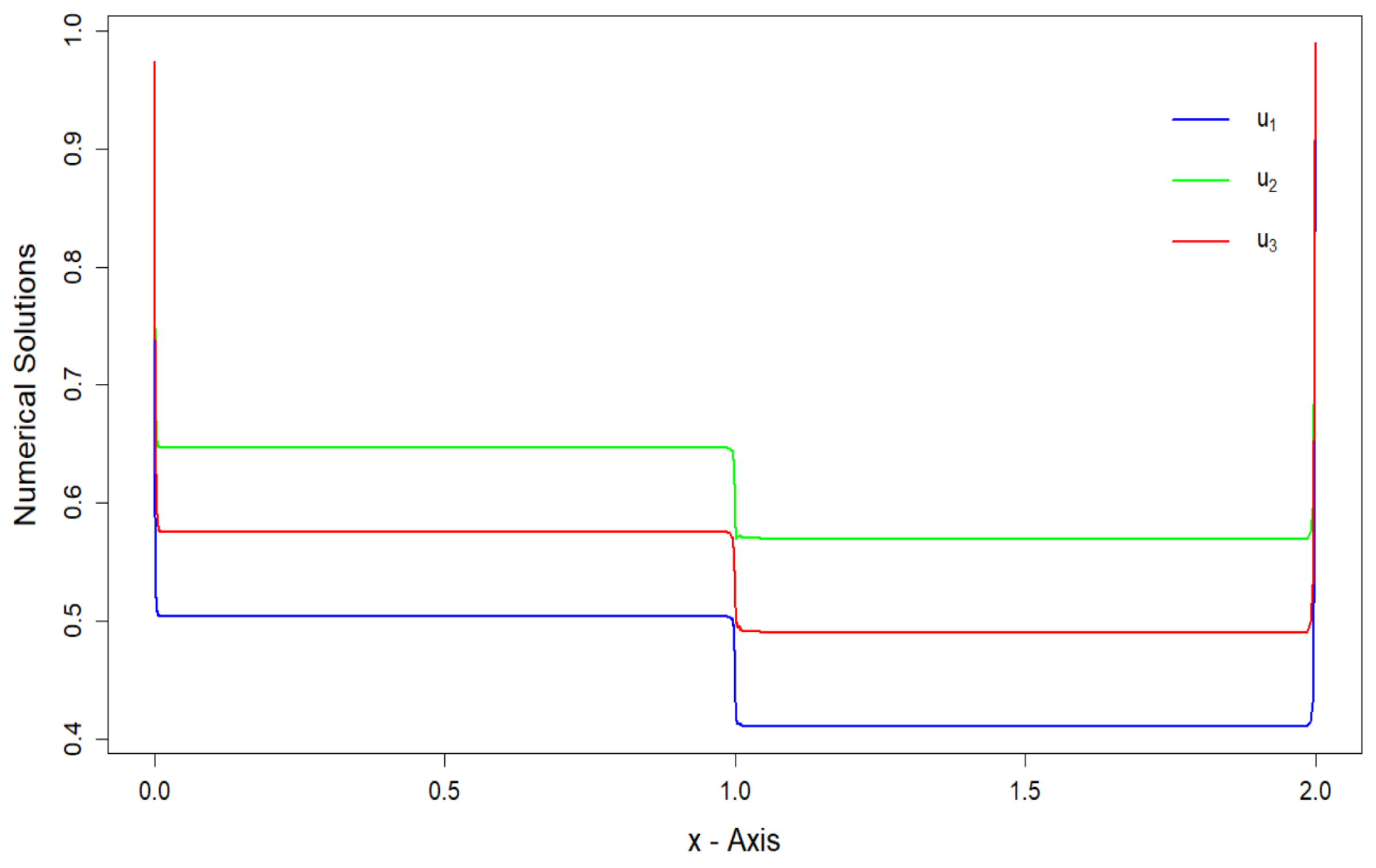
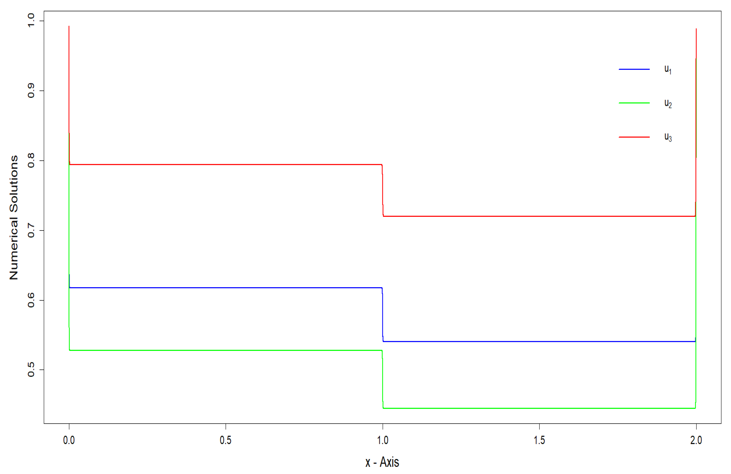
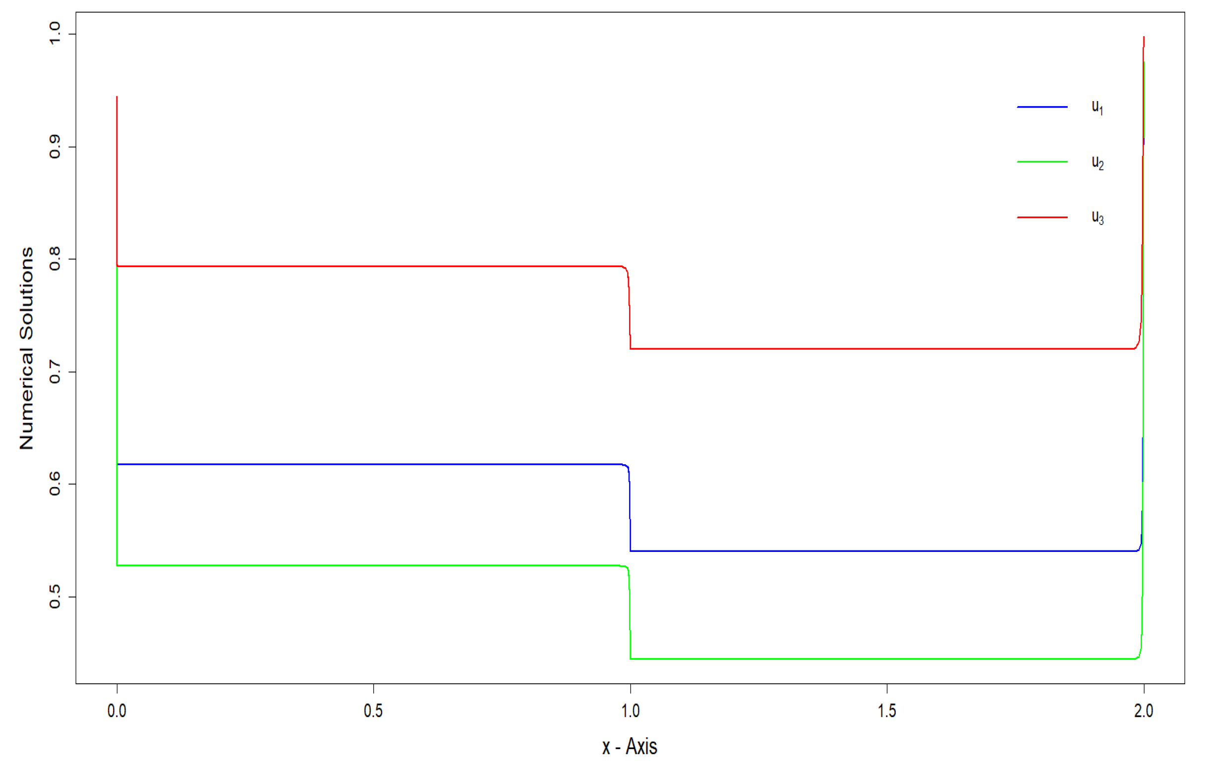
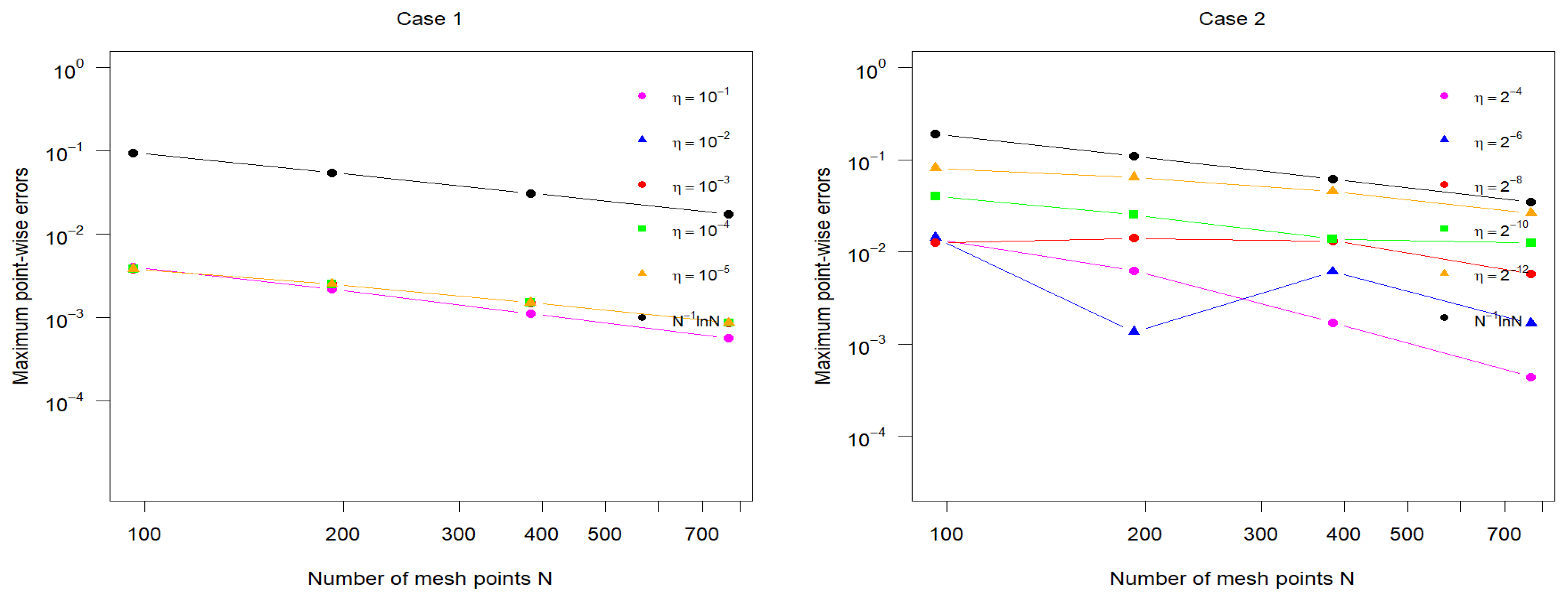
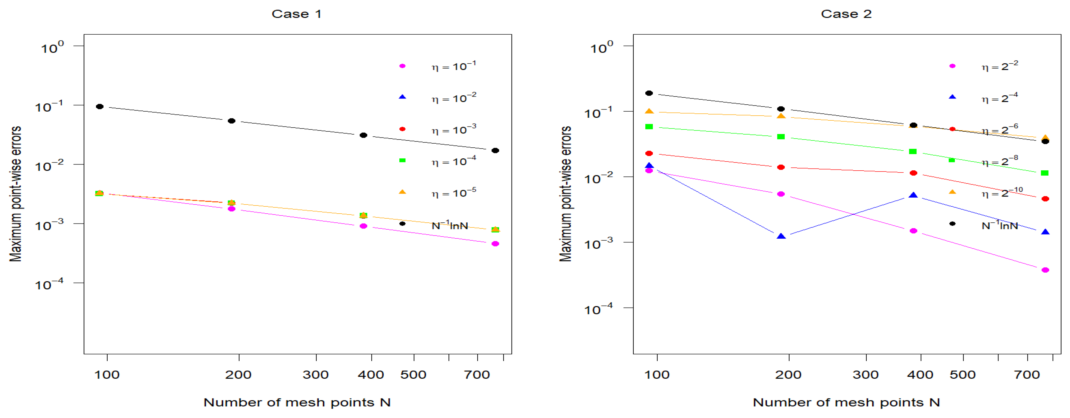
To evaluate the order of convergence, maximum pointwise errors and error constants, a modified two-mesh algorithm was utilized. The results are summarized in Table 1, Table 2, Table 3 and Table 4. As the parameter $\eta$ decreases, the error stabilizes for each N, while the maximum pointwise error $D_N$ decreases and the observed order of convergence $p_N$ improves as N increases, confirming the theoretical predictions. Figure 1 and Figure 2 display the solution profiles for the n-system over the interval $(0,2)$ for Example in Section 12.1. Figure 3 and Figure 4 display the solution profiles for the n-system over the interval $(0,2)$ for Example in Section 12.2. In Figure 1 and Figure 3, corresponding to the condition ${\displaystyle \frac{{\mu }^2}{{ϵ}_i}}\le {\displaystyle \frac{\gamma }{\alpha }},$ boundary layers are observed for the components ${\mathfrak{u}}_i$ ($i=1,2,\cdots ,n$) near $\varkappa =0$, $\varkappa =1$ and $\varkappa =2$, which is consistent with the theoretical expectations. On the other hand, Figure 2 and Figure 4 illustrate the case where ${\displaystyle \frac{{\mu }^2}{{ϵ}_j}}\ge {\displaystyle \frac{\gamma }{\alpha }}.$ Here, layers are observed for ${\mathfrak{u}}_i$ near $\varkappa =0$, while boundary layers emerge near $\varkappa =2$ and are delayed near $\varkappa =1$. Log–log plots effectively illustrate the relationship between the number of mesh points N and the maximum pointwise errors, offering a clear depiction of convergence behavior. Figure 5 and Figure 6 present the maximum pointwise errors for different $\eta$ values in Cases 1 and 2, demonstrating how the error decreases as N increases. These plots validate theoretical predictions and emphasize the impact of $\eta$ on the accuracy of the numerical method.

Table 1. For Example in Section 12.1. Values of $D_{\epsilon }^N,D^N,p^N,p^{*}$ and $C_{p^{*}}^N$ when ${ϵ}_1={\displaystyle \frac{\eta }{32}},{ϵ}_2={\displaystyle \frac{\eta }{16}},{ϵ}_3={\displaystyle \frac{\eta }{8}},\mu ={\displaystyle \frac{\eta }{8}}$ for $\alpha {\mu }^2\le \gamma {ϵ}_i$.

$\mathit{\eta }$	Number of Mesh Points $\mathit{N}$
	96	192	384	768
$0.1\times {10}^0$	$0.4050\times {10}^{-2}$	$0.2201\times {10}^{-2}$	$0.1123\times {10}^{-2}$	$0.5639\times {10}^{-3}$
$0.1\times {10}^{-1}$	$0.3832\times {10}^{-2}$	$0.2522\times {10}^{-2}$	$0.1509\times {10}^{-2}$	$0.8641\times {10}^{-3}$
$0.1\times {10}^{-2}$	$0.3832\times {10}^{-2}$	$0.2522\times {10}^{-2}$	$0.1509\times {10}^{-2}$	$0.8641\times {10}^{-3}$
$0.1\times {10}^{-3}$	$0.3832\times {10}^{-2}$	$0.2522\times {10}^{-2}$	$0.1509\times {10}^{-2}$	$0.8641\times {10}^{-3}$
$0.1\times {10}^{-4}$	$0.3832\times {10}^{-2}$	$0.2522\times {10}^{-2}$	$0.1509\times {10}^{-2}$	$0.8641\times {10}^{-3}$
$D^N$	$0.4050\times {10}^{-2}$	$0.2522\times {10}^{-2}$	$0.1509\times {10}^{-2}$	$0.8641\times {10}^{-3}$
$p^N$	$0.6828\times {10}^0$	$0.7408\times {10}^0$	$0.8049\times {10}^0$
$C_p^N$	$0.2424\times {10}^0$	$0.2424\times {10}^0$	$0.2329\times {10}^0$	$0.2140\times {10}^0$
The order of convergence $p^{*}=$ $0.6828\times {10}^0$
Computed error constant, $C_{p^{*}}^N=$ $0.2424\times {10}^0$

Table 2. For Example in Section 12.1. Values of $D_{\epsilon }^N,D^N,p^N,p^{*}$ and $C_{p^{*}}^N$ when ${ϵ}_1={\displaystyle \frac{\eta }{64}},{ϵ}_2={\displaystyle \frac{\eta }{32}},{ϵ}_3={\displaystyle \frac{\eta }{16}},\mu ={\displaystyle \frac{\eta }{4}}$ for $\alpha {\mu }^2\ge \gamma {ϵ}_j$.

$\mathit{\eta }$	Number of Mesh Points $\mathit{N}$
	96	192	384	768
$0.625\times {10}^{-1}$	$0.1369\times {10}^{-1}$	$0.6205\times {10}^{-2}$	$0.1707\times {10}^{-2}$	$0.4365\times {10}^{-3}$
$0.156\times {10}^{-1}$	$0.1420\times {10}^{-1}$	$0.1353\times {10}^{-2}$	$0.6080\times {10}^{-2}$	$0.1669\times {10}^{-2}$
$0.391\times {10}^{-2}$	$0.1258\times {10}^{-1}$	$0.1401\times {10}^{-1}$	$0.1317\times {10}^{-1}$	$0.5811\times {10}^{-2}$
$0.977\times {10}^{-3}$	$0.4006\times {10}^{-1}$	$0.2536\times {10}^{-1}$	$0.1383\times {10}^{-1}$	$0.1242\times {10}^{-1}$
$0.244\times {10}^{-3}$	$0.8087\times {10}^{-1}$	$0.6491\times {10}^{-1}$	$0.4528\times {10}^{-1}$	$0.2625\times {10}^{-1}$
$D^N$	$0.8087\times {10}^{-1}$	$0.6491\times {10}^{-1}$	$0.4528\times {10}^{-1}$	$0.2625\times {10}^{-1}$
$p^N$	$0.3170\times {10}^0$	$0.5195\times {10}^0$	$0.7862\times {10}^0$
$C_p^N$	$0.1742\times {10}^1$	$0.1742\times {10}^1$	$0.1514\times {10}^1$	$0.1093\times {10}^0$
The order of convergence $p^{*}=$ $0.3170\times {10}^0$
Computed error constant, $C_{p^{*}}^N=$ $0.1742\times {10}^1$

Table 3. For Example in Section 12.2. Values of $D_{\epsilon }^N,D^N,p^N,p^{*}$ and $C_{p^{*}}^N$ when ${ϵ}_1={\displaystyle \frac{\eta }{32}},{ϵ}_2={\displaystyle \frac{\eta }{16}},{ϵ}_3={\displaystyle \frac{\eta }{8}},\mu ={\displaystyle \frac{\eta }{8}}$ for $\alpha {\mu }^2\le \gamma {ϵ}_i$.

$\mathit{\eta }$	Number of Mesh Points $\mathit{N}$
	96	192	384	768
$0.1\times {10}^0$	$0.3314\times {10}^{-2}$	$0.1772\times {10}^{-2}$	$0.9087\times {10}^{-3}$	$0.4569\times {10}^{-3}$
$0.1\times {10}^{-1}$	$0.3220\times {10}^{-2}$	$0.2227\times {10}^{-2}$	$0.1359\times {10}^{-2}$	$0.7837\times {10}^{-3}$
$0.1\times {10}^{-2}$	$0.3220\times {10}^{-2}$	$0.2227\times {10}^{-2}$	$0.1359\times {10}^{-2}$	$0.7837\times {10}^{-3}$
$0.1\times {10}^{-3}$	$0.3220\times {10}^{-2}$	$0.2226\times {10}^{-2}$	$0.1359\times {10}^{-2}$	$0.7837\times {10}^{-3}$
$0.1\times {10}^{-4}$	$0.3220\times {10}^{-2}$	$0.2226\times {10}^{-2}$	$0.1359\times {10}^{-2}$	$0.7837\times {10}^{-3}$
$D^N$	$0.3314\times {10}^{-2}$	$0.2227\times {10}^{-2}$	$0.1359\times {10}^{-2}$	$0.7837\times {10}^{-3}$
$p^N$	$0.5734\times {10}^0$	$0.7119\times {10}^0$	$0.7947\times {10}^0$
$C_p^N$	$0.1384\times {10}^0$	$0.1384\times {10}^0$	$0.1257\times {10}^0$	$0.1078\times {10}^0$
The order of convergence $p^{*}=$ $0.5734\times {10}^0$
Computed error constant, $C_{p^{*}}^N=$ $0.1384\times {10}^0$

Table 4. For Example in Section 12.2. Values of $D_{\epsilon }^N,D^N,p^N,p^{*}$ and $C_{p^{*}}^N$ when ${ϵ}_1={\displaystyle \frac{\eta }{64}},{ϵ}_2={\displaystyle \frac{\eta }{32}},{ϵ}_3={\displaystyle \frac{\eta }{16}},\mu ={\displaystyle \frac{\eta }{4}}$ for $\alpha {\mu }^2\ge \gamma {ϵ}_j$.

$\mathit{\eta }$	Number of Mesh Points $\mathit{N}$
	96	192	384	768
$0.625\times {10}^{-1}$	$0.1250\times {10}^{-1}$	$0.5441\times {10}^{-2}$	$0.1502\times {10}^{-2}$	$0.3815\times {10}^{-3}$
$0.156\times {10}^{-1}$	$0.1468\times {10}^{-1}$	$0.1218\times {10}^{-2}$	$0.5175\times {10}^{-2}$	$0.1418\times {10}^{-2}$
$0.391\times {10}^{-2}$	$0.2277\times {10}^{-1}$	$0.1405\times {10}^{-1}$	$0.1151\times {10}^{-1}$	$0.4628\times {10}^{-2}$
$0.977\times {10}^{-3}$	$0.5803\times {10}^{-1}$	$0.4096\times {10}^{-1}$	$0.2434\times {10}^{-1}$	$0.1133\times {10}^{-1}$
$0.244\times {10}^{-3}$	$0.9866\times {10}^{-1}$	$0.8324\times {10}^{-1}$	$0.5966\times {10}^{-1}$	$0.3902\times {10}^{-1}$
$D^N$	$0.9866\times {10}^{-1}$	$0.8324\times {10}^{-1}$	$0.5966\times {10}^{-1}$	$0.3902\times {10}^{-1}$
$p^N$	$0.2451\times {10}^0$	$0.4805\times {10}^0$	$0.6124\times {10}^0$
$C_p^N$	$0.1933\times {10}^1$	$0.1933\times {10}^1$	$0.1642\times {10}^1$	$0.1272\times {10}^0$
The order of convergence $p^{*}=$ $0.2451\times {10}^0$
Computed error constant, $C_{p^{*}}^N=$ $0.1933\times {10}^1$

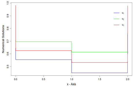
Figure 1. The graphical representation of numerical solutions for Example in Section 12.1 for the following case: $\alpha {\mu }^2\le \gamma {ϵ}_i$.

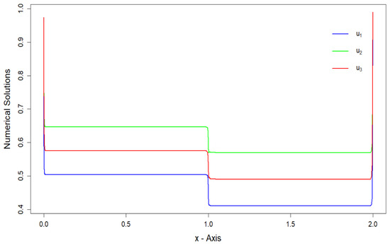
Figure 2. The graphical representation of numerical solutions for Example in Section 12.1 for the following case: $\alpha {\mu }^2\ge \gamma {ϵ}_j$.

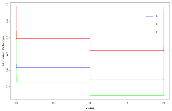
Figure 3. The graphical representation of numerical solutions for Example in Section 12.2 for the following case: $\alpha {\mu }^2\le \gamma {ϵ}_i$.

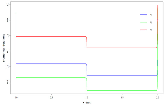
Figure 4. The graphical representation of numerical solutions for Example in Section 12.2 for the following case: $\alpha {\mu }^2\ge \gamma {ϵ}_j$.

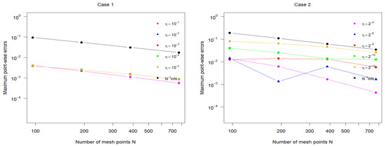
Figure 5. For The graphical representation of maximum pointwise errors for Example in Section 12.1 for different $\eta$ values for Cases 1 and 2.

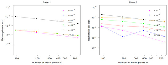
Figure 6. The graphical representation of maximum pointwise errors for Example in Section 12.2 for different $\eta$ values for Cases 1 and 2.

13. Conclusions

This paper presented a robust fitted mesh finite difference method for solving a system of two-parameter ‘n’ singularly perturbed delay differential equations of the convection–reaction–diffusion type. The method leverages a piecewise uniform Shishkin mesh to address the intricate challenges posed by small perturbation parameters and delay terms across multiple equations. Our theoretical analysis demonstrates that the proposed scheme attains nearly first-order convergence in the maximum norm, uniformly with respect to the perturbation parameters. Numerical experiments confirm the method’s robustness and accuracy, demonstrating its capability to resolve boundary layers with precision across a system of equations. This work marks a significant advancement in numerical techniques for SPDDEs, emphasizing the critical importance of developing parameter-uniform methods to address the unique challenges posed by systems of equations with multiple layers and delays. Future investigations could focus on extending these methods to enhance the computational efficiency, improve convergence rates and handle more intricate systems encountered in real-world applications.

References

- Bhatti, M.M.; Alamri, S.Z.; Ellahi, R.; Abdelsalam, S.I. Intra-uterine particle-fluid motion through a compliant asymmetric tapered channel with heat transfer. J. Therm. Anal. Calorim. 2021, 144, 2259–2267. [Google Scholar] [CrossRef]
- Glizer, V. Asymptotic analysis and solution of a finite-horizon H∞ control problem for singularly-perturbed linear systems with small state delay. J. Optim. Theory Appl. 2003, 117, 295–325. [Google Scholar] [CrossRef]
- Miller, J.J.H.; O’Riordan, E.; Shishkin, G.I. Fitted Numerical Methods for Singular Perturbation Problems: Error Estimates in the Maximum Norm for Linear Problems in One and Two Dimensions; World Scientific: Singapore, 2012. [Google Scholar]
- Doolan, E.P.; Miller, J.J.H.; Schilders, W.H.A. Uniform Numerical Methods for Problems with Initial and Boundary Layers; Boole Press: Dublin, Ireland, 1980. [Google Scholar]
- Cen, Z. Parameter-uniform finite difference scheme for a system of coupled singularly perturbed convection-diffusion equations. Int. J. Comput. Math. 2005, 82, 177–192. [Google Scholar] [CrossRef]
- Gracia, J.L.; O’Riordan, E.; Pickett, M.L. A parameter robust second order numerical method for a singularly perturbed two-parameter problem. Appl. Numer. Math. 2006, 56, 962–980. [Google Scholar] [CrossRef]
- O’Malley, R.E. Two-parameter singular perturbation problems for second-order equations. J. Math. Mech. 1967, 16, 1143–1164. [Google Scholar]
- O’Riordan, E.; Pickett, M.L.; Shishkin, G.I. Singularly perturbed problems modeling reaction-convection-diffusion processes. Comput. Methods Appl. Math. 2003, 3, 424–442. [Google Scholar] [CrossRef]
- Raja, V.; Geetha, N.; Mahendran, R.; Senthilkumar, L.S. Numerical solution for third order singularly perturbed turning point problems with integral boundary condition. J. Appl. Math. Comput. 2025, 71, 829–849. [Google Scholar] [CrossRef]
- Besova, M.; Kachalov, V. Axiomatic approach in the analytic theory of singular perturbations. Axioms 2020, 9, 9. [Google Scholar] [CrossRef]
- Daba, I.T.; Melesse, W.G.; Gelu, F.W.; Kebede, G.D. An efficient numerical approach for singularly perturbed time delayed parabolic problems with two parameters. BMC Res. Notes 2024, 17, 158. [Google Scholar] [CrossRef]
- Woldaregay, M.M. Solving singularly perturbed delay differential equations via fitted mesh and exact difference method. Res. Math. 2022, 9, 2109301. [Google Scholar] [CrossRef]
- Kalaiselvan, S.S.; Miller, J.J.H.; Sigamani, V. A parameter uniform numerical method for a singularly perturbed two-parameter delay differential equation. Appl. Numer. Math. 2019, 145, 90–110. [Google Scholar] [CrossRef]
- Nagarajan, S. A parameter robust fitted mesh finite difference method for a system of two reaction-convection-diffusion equations. Appl. Numer. Math. 2022, 179, 87–104. [Google Scholar] [CrossRef]
- Arthur, J.; Chatzarakis, G.E.; Panetsos, S.L.; Mathiyazhagan, J.P. A robust-fitted-mesh-based finite difference approach for solving a system of singularly perturbed convection–diffusion delay differential equations with two parameters. Symmetry 2025, 17, 68. [Google Scholar] [CrossRef]
- Mathiyazhagan, P.; Sigamani, V.; Miller, J.J.H. Second order parameter-uniform convergence for a finite difference method for a singularly perturbed linear reaction-diffusion system. Math. Commun. 2010, 15, 587–612. [Google Scholar]
- Arthur, J.; Mathiyazhagan, J.P.; Chatzarakis, G.E.; Panetsos, S.L. Advanced Fitted Mesh Finite Difference Strategies for Solving ’n’ Two-Parameter Singularly Perturbed Convection-Diffusion System. Axioms 2025, 14, 171. [Google Scholar] [CrossRef]
- Farrell, P.; Hegarty, A.; Miller, J.M.; O’Riordan, E.; Shishkin, G.I. Robust Computational Techniques for Boundary Layers, 1st ed.; Chapman and Hall/CRC: Boca Raton, FL, USA, 2000. [Google Scholar] [CrossRef]
Disclaimer/Publisher’s Note: The statements, opinions and data contained in all publications are solely those of the individual author(s) and contributor(s) and not of MDPI and/or the editor(s). MDPI and/or the editor(s) disclaim responsibility for any injury to people or property resulting from any ideas, methods, instructions or products referred to in the content. |
© 2025 by the authors. Licensee MDPI, Basel, Switzerland. This article is an open access article distributed under the terms and conditions of the Creative Commons Attribution (CC BY) license (https://creativecommons.org/licenses/by/4.0/).