On High-Order Runge–Kutta Pairs for Linear Inhomogeneous Problems

Abstract

This paper introduces a novel Runge–Kutta (RK) pair of orders $8\left(6\right)$ designed specifically for solving linear inhomogeneous initial value problems (IVPs) with constant coefficients. The proposed method requires only 11 stages per iteration, a significant improvement over conventional RK pairs of orders $8\left(7\right)$, which typically demand 13 stages. The reduction in stages is achieved by leveraging a smaller set of order conditions tailored to linear inhomogeneous problems, where traditional simplification techniques are not applicable. To address the complexity of deriving such methods, the authors employ the Differential Evolution algorithm, a global optimization technique, to solve the resulting system of equations. The new RK pair, named NEW8(6)Lin, is tested on several benchmark problems, including scalar, linear inhomogeneous, and larger systems, demonstrating a superior performance in terms of accuracy and computational efficiency. The method’s high phase-lag accuracy and efficiency make it particularly suitable for problems requiring high precision over extended intervals. The coefficients of the method are provided with high precision, enabling direct implementation in computational environments like Mathematica. The results highlight the method’s potential as a robust tool for solving linear inhomogeneous IVPs, offering a balance between computational cost and accuracy. This work contributes to the ongoing development of specialized numerical methods for differential equations, particularly in scenarios where traditional approaches struggle with efficiency or stability.

1. Introduction

The dynamics of modern computational methods have revolutionized the field of numerical analysis, enabling researchers to address previously intractable problems. Recent advances have highlighted the versatility of techniques in applied mathematics, particularly when solving high-dimensional differential equations. The integration of novel algorithms, such as adaptive mesh refinement and machine-learning-inspired optimization, underscores the rapid evolution of computational science.

Furthermore, interdisciplinary applications, ranging from quantum mechanics to astrophysics, demand precision and computational efficiency. For example, the study of Bose–Einstein condensates often relies on numerically solving nonlinear Schrödinger equations, while stellar structure models necessitate the solution of Lane–Emden equations under complex boundary conditions.

In parallel, the rise of hybrid numerical–analytical techniques has offered an avenue for balancing theoretical rigor with computational practicality. Hybrid methodologies are particularly effective in scenarios where traditional methods struggle, such as in the presence of singularities or discontinuities.

Moreover, the role of numerical methods in modeling real-world phenomena cannot be overstated. Applications in geophysics, such as simulating seismic wave propagation, and in climate modeling, such as solving Navier–Stokes equations for atmospheric flow, exemplify their profound impact.

This introduction aims to situate the subsequent analysis within this broader computational landscape. By contextualizing our study within these emerging trends, we demonstrate the relevance and applicability of the proposed methods to cutting-edge scientific challenges.

The resolution of initial value problems (IVPs) remains fundamental in the numerical analysis community. Such problems often arise in scenarios where the state of a dynamic system evolves according to specified initial conditions. Applications include modeling the trajectory of celestial bodies, simulating population dynamics, and studying chemical reaction kinetics.

The first-order IVP is represented as follows:

$$y^{\prime }=f(x,y),y\left(x_0\right)=y_0\in {\mathbb{R}}^m,x\in [x_0,x_e],$$

(1)

where $f:\mathbb{R}\times {\mathbb{R}}^m\to {\mathbb{R}}^m.$

Equation (1) encompasses a wide range of applications, from the ones mentioned before.

Our research team is focused on devising specialized algorithms for distinct scenarios of problem (1). These include the development of Runge-Kutta-Nystrom [1,2] and Numerov techniques tailored for second-order equations [3], as well as multistep approaches [4].

In this work, we address the linear inhomogeneous Initial Value Problem (IVP), expressed as follows:

$$y^{\prime }\left(x\right)=Ly\left(x\right)+g\left(x\right),y\left(x_0\right)=y_0,$$

(2)

where $L\in {\mathbb{R}}^{m\times m}$ and $g:\mathbb{R}\to {\mathbb{R}}^m$. Such systems typically arise when the Method of Lines is employed to solve linear wave equations.

Linear homogeneous systems, on the other hand, provide a framework for describing a variety of physical systems governed by linear dynamics. These include models in control theory, electrical circuit analysis, and quantum mechanics. The incorporation of a linear operator L alongside an inhomogeneous term $g\left(x\right)$ introduces additional complexity, necessitating robust numerical methods for accurate solutions.

Despite the wide range of existing numerical techniques, challenges persist. Stability and accuracy are paramount when solving IVPs over extended intervals or when dealing with stiff equations. Similarly, for linear systems, ensuring computational efficiency while preserving the structure of the solution is a critical goal, particularly for large-scale problems.

This work aims to address these challenges by enhancing established numerical methods and tailoring them to the specific needs of problems (1) and (2). The proposed approach not only improves accuracy, but also offers greater flexibility in handling a diverse array of applications.

Runge–Kutta methods are explicit or implicit techniques that compute successive approximations by evaluating the function $Ly\left(x\right)+g\left(x\right)$ at specific points within an interval. For instance, the classical fourth-order Runge–Kutta method iteratively refines the solution using a weighted average of function evaluations at intermediate stages. These methods are favored for their simplicity and accuracy in non-stiff scenarios.

In cases where stiffness is present—characterized by rapidly varying eigenvalues of L—implicit methods such as backward Euler or implicit Runge–Kutta variants become essential. These techniques maintain stability over larger step sizes, which is critical for computational efficiency.

Beyond Runge–Kutta, matrix exponentiation methods are particularly well-suited for linear systems. Techniques like Magnus expansion or Krylov subspace approximations exploit the linearity of L, enabling direct computation of the propagator $e^{Lx}$.

Overall, the numerical treatment of problem (2) leverages a balance between computational efficiency and stability, with method selection guided by the specific characteristics of the system being modeled.

Shampine was among the pioneers to tackle systems of first-order IVPs [5], employing a fourth-order scheme by England [6] and error estimation through Richardson extrapolation (doubling). Enright extended this work in the late 1970s [7]. Subsequently, Zingg and Chisholm [8] introduced various Runge–Kutta methods of orders four, five, and six tailored to problems like (2).

Among the widely utilized numerical approaches for solving (1) are Runge–Kutta (RK) pairs, which are described by the following generalized Butcher tableau [9,10]:

$$\begin{array}{cc}\hfill c & \overline{) A}\hfill \\ & \overline{) \begin{array}{c}b\\ \widehat{b}\end{array}}\hfill \end{array}$$

where $b^T$, ${\widehat{b}}^T$, and $c\in {\mathbb{R}}^s$, with $A\in {\mathbb{R}}^{s\times s}$ being strictly lower triangular. To advance the numerical solution from $(x_n,y_n)$ to $x_{n+1}=x_n+h_n$, two approximations, $y_{n+1}$ and ${\widehat{y}}_{n+1}$, are computed for $y\left(t_{n+1}\right)$. These approximations are of orders p and q, respectively, with $q<p$, and are expressed as follows:

$$y_{n+1}=y_n+h_n\sum _{i=1}^s{b}_i{f}_{ni},$$

(3)

and

$${\widehat{y}}_{n+1}=y_n+h_n\sum _{i=1}^s{\widehat{b}}_i{f}_{ni},$$

where the intermediate values are defined as follows:

$$f_{ni}=f(x_n+c_i{h}_n,y_n+h_n\sum _{j=1}^{i-1}{a}_{ij}{f}_{nj}),$$

(4)

for $i=1$, $2,\dots ,s\ge p$. Almost every RK method adheres to the simplifying condition:

$$A·e=c,e={\left[1,1,1,\dots ,1,1\right]}^T\in {\mathbb{R}}^s.$$

(5)

The estimation of the local error [11] is given by the following:

$${ϵ}_{n+1}=∥y_{n+1}-{\widehat{y}}_{n+1}∥·h^{p-q-1},$$

and serves as the foundation for the adaptive step-size control algorithm:

$$h_{n+1}=0.90·h_n·{\left({\displaystyle \frac{\epsilon }{{ϵ}_{n+1}}}\right)}^{1/p},$$

where $\epsilon$ denotes a user-defined tolerance level. This formulation is employed regardless of whether $\epsilon <{ϵ}_{n+1}$. In such cases, $h_{n+1}$ is effectively a smaller adjusted value of $h_n$. For further elaboration on this methodology, refer to [11].

In general, a non-stiff linear inhomogeneous IVP benefits from high-order Runge–Kutta schemes because they provide greater accuracy per step, reducing total steps and error accumulation while efficiently handling complex forcing terms and solution behavior. This has already been shown in [12] where a seventh order method outperformed other lower order methods.

The study presents a novel Runge–Kutta (RK) pair of orders 8(6) tailored for linear inhomogeneous initial value problems (IVPs) with constant coefficients. Traditional RK pairs of similar accuracy, such as order 8(7), require more computational effort, typically 13 stages per iteration, whereas the proposed method achieves a comparable accuracy with only 11 stages. This reduction is possible through an optimized set of order conditions specific to linear inhomogeneous systems.

In the existing literature, higher-order RK methods have been extensively developed, but they often lack efficiency for linear inhomogeneous problems due to unnecessary constraints inherited from general RK formulations. Prior research focused on stiff solvers, symplectic integrators, and adaptive RK methods, yet specialized RK pairs for linear inhomogeneous IVPs remain scarce. This paper fills that gap by introducing a globally optimized RK pair using Differential Evolution, significantly improving the accuracy and computational cost.

By systematically addressing these gaps, the paper demonstrates clear originality in numerical method development, making a compelling case for its relevance in solving large-scale IVPs, wave equations, and other applied problems where existing methods struggle with efficiency.

2. RK Methods and Rooted Trees Theory

2.1. Expansions of Taylor Series

For simplicity, we assume $x^{\prime }=1$, transforming (1) into the autonomous form $y^{\prime }=y\left(x\right)$, which is often more practical and generality is preserved also. When the p-th order RK method (3) and (4) is applied to this reformulated problem, the goal is essentially to approximate the equivalent Taylor series system:

$$y\left(x_{n+1}\right)\approx y\left(x_n\right)+h{y}^{\prime }\left(x_n\right)+{\displaystyle \frac{1}{2!}}{y}^{″}\left(x_n\right)+\cdots +{\displaystyle \frac{1}{p!}}{y}^{\left(p\right)}\left(x_n\right),$$

(6)

Expanding $f_{ni}$ around $\left(x_n,y_n\right)$ and substituting into (3), we obtain:

$$y_{n+1}=y_n+h{q}_{11}{y}_n^{\prime }+h^2{q}_{21}{y}_n^{″}+h^3\left(q_{31}{y}^{\prime }f+q_{32}{f}^{″}{f}^2\right)+\cdots ,$$

(7)

where $q_{ij}$ are functions exclusively of the coefficients b, c, and A.

We may verify,

$$\begin{array}{ccc}\hfill y^{″}& =& {\displaystyle \frac{\partial f\left(y\left(t\right)\right)}{\partial t}}={\displaystyle \frac{\partial f}{\partial y}}f=f^{\prime }f,\hfill \\ \hfill y^{‴}& =& f^{″}·\left(f,f\right)+{\displaystyle \frac{\partial f}{\partial y}}·{\displaystyle \frac{\partial f}{\partial y}}·f=f^{″}·\left(f,f\right)+f^{\prime }{f}^{\prime }f,\hfill \\ \hfill y^{\prime \prime \prime \prime }& =& f^{‴}·\left(f,f,f\right)+{\displaystyle \frac{\partial f}{\partial y}}·{\displaystyle \frac{\partial f}{\partial y}}·{\displaystyle \frac{\partial f}{\partial y}}·f\hfill \\ & & +3·f^{″}\left({\displaystyle \frac{\partial f}{\partial y}}·f,f\right)+{\displaystyle \frac{\partial f}{\partial y}}·f^{″}·\left(f,f\right)\hfill \\ & =& f^{‴}·\left(f,f,f\right)+f^{\prime }{f}^{\prime }{f}^{\prime }f+3f^{″}·\left(f^{\prime }f,f\right)+f^{\prime }{f}^{″}\left(f,f\right),\hfill \\ & & \cdots \hfill \end{array}$$

where the elementary differentials $f^{″}\left(f,f\right),f^{″}\left(f,f,f\right)$, $f^{\prime }{f}^{″}\left(f,f\right)$ and $f^{″}\left(f^{\prime }f,f\right)$ come from the corresponding Frechet derivatives, [13] (p. 158).

As an example, take:

$$f={[y_2{y}_1^2+y_1,y_2{y}_1^3+y_2^3{y}_1]}^T\in {\mathbb{R}}^2.$$

Then, the Jacobian is

$$f^{\prime }=\left(\begin{array}{cc}2y_1{y}_2+1& y_1^2\\ y_2^3+3y_1^2{y}_2& y_1^3+3y_2^2{y}_1\end{array}\right)\in {\mathbb{R}}^{2\times 2},$$

while

$$f^{″}=\left(\begin{array}{cccc}2y_2& 2y_1& 2y_1& 0\\ 6y_1{y}_2& 3y_1^2+3y_2^2& 3y_1^2+3y_2^2& 6y_1{y}_2\end{array}\right)\in {\mathbb{R}}^{2\times 4},$$

and

$$f^{″}·(f,f)=\left(\begin{array}{c}2y_1^2{y}_2\left(y_1{y}_2+1\right)\left(2y_1^3+2y_2^2{y}_1+y_2{y}_1+1\right)\\ 6y_1^2{y}_2\left(y_1^3+y_2^2{y}_1+y_2{y}_1+1\right)\left(y_2^4+y_1^2{y}_2^2+y_1^2{y}_2+y_1\right)]\end{array}\right)\in {\mathbb{R}}^2,$$

as $(f,f)\in {\mathbb{R}}^4$, etc.

Then, we match (6) and (7) and arrive at

$$\begin{array}{c}y\left(x_{n+1}\right)-y_{n+1}=h\left({\varphi }_{11}-1\right)f+h^2\left({\varphi }_{21}-{\displaystyle \frac{1}{2}}\right){\displaystyle \frac{\partial f}{\partial y}}f+\hfill \\ h^3\left(\left({\varphi }_{31}-{\displaystyle \frac{1}{6}}\right)f^T·{\displaystyle \frac{{\partial }^{2}f}{\partial y^2}}·f+\left({\varphi }_{32}-{\displaystyle \frac{1}{6}}\right){\displaystyle \frac{\partial f}{\partial y}}·{\displaystyle \frac{\partial f}{\partial y}}·f\right)+\cdots \hfill \end{array},$$

(8)

with various $\varphi$ polynomial functions of the coefficients. Imposing the conditions $q_{11}={\varphi }_{11}-1=b·e-1=0$, $q_{21}={\varphi }_{21}-{\displaystyle \frac{1}{2}}=b·c-{\displaystyle \frac{1}{2}}=0,$$q_{31}={\varphi }_{31}-{\displaystyle \frac{1}{6}}=0$, and $q_{32}={\varphi }_{32}-{\displaystyle \frac{1}{6}}=0$, we derive the set of equations required to construct a third-order method. The algebraic constraints, up to fifth order, are listed in the first column of

Table 1. The conditions required for Runge–Kutta methods of orders 1 through 5 are presented. In the rightmost column, we list the remaining constraints specific to (2).

Order Conditions	Elementary Differential	Valid for (2)
$q_{11}=b·e-1$	$f$	OK
$q_{21}=b·c-\frac{1}{2}$	$f^{\prime }f$	OK
$q_{31}=\frac{1}{2}b·c^2-\frac{1}{6}$	$f^{″}·(f,f)$	OK
$q_{32}=b·A·c-\frac{1}{6}$	$f^{\prime }·f^{\prime }·f$	OK
$q_{41}=\frac{1}{6}b·c^3-\frac{1}{24}$	$f^{‴}·(f,f,f)$	OK
$q_{42}=\frac{1}{2}b·A·c^2-\frac{1}{24}$	$f^{\prime }·f^{″}·(f,f)$	OK
$q_{43}=b·\left(c\ast (A·c)\right)-\frac{1}{8}$	$f^{″}·(f^{\prime }·f,f)$	no
$q_{44}=b·A^2·c-\frac{1}{24}$	$f^{\prime }·f^{\prime }·f^{\prime }·f$	OK
$q_{51}=\frac{1}{24}b·c^4-\frac{1}{120}$	$f^{\prime \prime \prime \prime }·(f,f,f,f)$	OK
$q_{52}=b·\left(c^2\ast (A·c)\right)-\frac{1}{20}$	$f^{‴}·(f^{\prime }·f,f,f)$	no
$q_{53}=\frac{1}{2}b·\left(c\ast (A·c^2)\right)-\frac{1}{30}$	$f^{″}·(f^{″}·\left(f,f\right),f)$	no
$q_{54}=b·\left(c\ast (A^2·c)\right)-\frac{1}{30}$	$f^{″}·(f^{\prime }·f^{\prime }·f,f)$	no
$q_{55}=\frac{1}{2}b·{\left(A·c\right)}^2-\frac{1}{40}$	$f^{″}·(f^{\prime }·f,f^{\prime }·f)$	no
$q_{56}=\frac{1}{6}b·A·c^3-\frac{1}{120}$	$f^{\prime }·f^{‴}·(f,f,f)$	OK
$q_{57}=b·A·\left(c\ast (A·c)\right)-\frac{1}{40}$	$f^{\prime }·f^{″}·(f^{\prime }·f,f)$	no
$q_{58}=\frac{1}{2}b·A^2·c^2-\frac{1}{120}$	$f^{\prime }·f^{\prime }·f^{″}(f,f)$	OK
$q_{59}=b·A^3·c-\frac{1}{120}$	$f^{\prime }·f^{\prime }·f^{\prime }·f^{\prime }·f$	OK

.

In this table, $c^2$ represents the element-wise product of the components in c. Similarly, ${(A·c)}^2$ indicates the corresponding element-wise multiplications of the entries of the vector $A·c$. As a result, $c^i$ refers to a vector where each element is the corresponding power i of the entries in c. These operations are always computed prior to others. Throughout the tables, element-wise vector multiplication is denoted by the symbol ∗. For example, $c^2=c\ast c$ and $c^3=\left(c^2\right)\ast c$. When ∗ is used, it holds lower precedence compared to other operations. Additionally, $c^0=e$, and we define $C=\mathrm{diag}\left(c\right)$.

The initial column of Table 1 enumerates the order conditions for Runge–Kutta methods up to the fifth order.

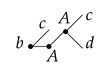
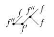
2.2. Trees and Rooted Trees

Equation (8) can be reformulated as

$$y\left(x_{n+1}\right)-x_{n+1}=\sum _{i=1}^{\infty }\sum _{\tau \in T_i}{h}^i{\displaystyle \frac{1}{\sigma \left(\tau \right)}}\left(\Phi \left(\tau \right)-{\displaystyle \frac{1}{\gamma \left(\tau \right)}}\right)F\left(\tau \right),$$

where $T_i$ represents the i-th order collection of rooted trees, $\sigma$ and $\gamma$ are integer-valued functions of $\tau$, $\Phi$ is a polynomial in A, b, and c, and F denotes an elementary differential [14].

A Runge–Kutta method attains an order p if and only if

$$X\left(\tau \right)={\displaystyle \frac{1}{\sigma \left(\tau \right)}}\left(\Phi \left(\tau \right)-{\displaystyle \frac{1}{\gamma \left(\tau \right)}}\right)=0,\tau \in T_i,\mathrm{for}i=1\left(1\right)p.$$

The above constitutes a system of conditions, linear in b and nonlinear in A and d (refer to Butcher [14] or Hairer, Nørsett, and Wanner [15] for details). The symbol $T^{\left(i\right)}$ signifies the vector containing all components of $X\left(T_i\right)$.

Each rooted tree $\tau$ uniquely aligns with an order condition, achieved by assigning b to the root, A to interior nodes, and d to the leaves. Using prefix multiplication, $\Phi \left(\tau \right)$ is constructed from these conditions. For instance, consider the rooted tree $\tilde{\tau }$ which produces $\Phi \left(\tilde{\tau }\right)=b·\left(c\ast \left(A^2·c^2\right)\right).$

In the same way, we obtain the related elementary differential. We associate every node with $f^{\left(\mu \right)}$ where $\mu$ is the number of successors of the node. For the leaves $f^{\left(0\right)}$ is comprehended as f. Working on the same tree as above, we have and conclude the elementary differential

$$F\left(\tilde{\tau }\right)=f^{″}\left(f,f^{\prime }{f}^{″}\left(f,f\right)\right).$$

The second column of Table 1 provides an interpretation of this relationship for order conditions up to five. For problems of type (2), $F\left(\tilde{\tau }\right)=0$. This happens because all elementary differentials (listed in the second column of Table 1) vanish whenever they involve a higher derivative of f enclosed in parentheses. Specifically, the following conditions hold:

$${\displaystyle \frac{{\partial }^{i}f}{\partial y^i}}=0,\mathrm{for}i>1,$$

and

$${\displaystyle \frac{{\partial }^{i+j}f}{\partial y^i\partial x^j}}=0,\mathrm{for}i\ge 1,j\ge 1.$$

The third column in Table 1 records the equations of condition that remain valid for (2) based on this observation.

Lastly, the coefficients of the truncation error (and thus the relevant order conditions) for orders $p\ge 2$ can now be expressed as follows:

$$q_{p,j}^{*}={\displaystyle \frac{1}{j!}}b·A^{(p-j-1)}·c^j-{\displaystyle \frac{1}{p!}},\mathrm{for}p-1\ge j\ge 1,$$

(9)

where $A^0$ denotes the identity matrix. For $p=1$, we obtain $q_{11}^{*}=be-1$.

Consequently, there are $p-1$-order conditions for every $p\ge 2$.

3. Derivation of the New Pairs

Here, we consider Runge–Kutta pairs of orders eight and six sharing 12 stages per step. A technique called FSAL (First Stage As Last) [16] is commonly used with these methods and only 11 stages are wasted in every step. We have $s=11$ and the parameters involved after (5) are 56. Namely,

$$c_2,c_3,\cdots ,c_{11},a_{32},a_{42},a_{43},\cdots ,a_{11,10},$$

and

$$b_6,b_4,b_5,b_1,b_7,b_8,b_9,b_{10},b_{11}{\widehat{b}}_1,{\widehat{b}}_4,\cdots ,{\widehat{b}}_{11}.$$

For the other coefficients, we assume

$$c_{11}=c_{12}=1,A·e=c,\mathrm{and}$$

$$a_{12,j}=b_j,j=1,2,\cdots ,11\left(\mathrm{FSAL}\right),$$

while we fix ${\widehat{b}}_{12}={\displaystyle \frac{1}{20}}\ne b_{12}=0.$ The specific choice of ${\widehat{b}}_{12}$ is relatively flexible. By selecting any $\lambda \ne 1$, we can construct

$$\widehat{\widehat{b}}=\lambda b+\left(1-\lambda \right)\widehat{b},$$

which serves as a new sixth-order weight vector [17].

It is worth noting that the above free parameters allow for the derivation of a method pair with orders of $8\left(6\right)$. This is achievable as an eighth-order method requires satisfying 29-order conditions, while the lower sixth-order method involves an additional 16 conditions. Table 1 provides 11 of the order conditions spanning orders 1–5. The remaining 18 conditions, pertaining to orders 6–8, can be deduced by analyzing (9) and are presented in

Table 2. The equations of condition for linear inhomogeneous Runge–Kutta methods for orders 6–8.

$b·A^4·c-\frac{1}{720},$	$\frac{1}{2}b·A^3·c^2-\frac{1}{720},$	$\frac{1}{6}b·A^2·c^3-\frac{1}{720},$
$\frac{1}{24}b·A·c^4-\frac{1}{720}$	$\frac{1}{120}b·c^5-\frac{1}{720},$	$b·A^5·c-\frac{1}{5040},$
$\frac{1}{2}b·A^4·c^2-\frac{1}{5040},$	$\frac{1}{6}b·A^3·c^3-\frac{1}{5040},$	$\frac{1}{24}b·A^2·c^4-\frac{1}{5040},$
$\frac{1}{120}b·A·c^5-\frac{1}{5040}$,	$\frac{1}{720}b·c^6-\frac{1}{5040}$	$q_{81}^{*}=b·A^6·c-\frac{1}{40320},$
$\frac{1}{2}b·A^5·c^2-\frac{1}{40320},$	$\frac{1}{6}b·A^4·c^3-\frac{1}{40320},$	$\frac{1}{24}b·A^3·c^4-\frac{1}{40320},$
$\frac{1}{120}b·A^2·c^5-\frac{1}{40320},$	$\frac{1}{720}b·A·c^6-\frac{1}{40320},$	$q_{87}^{*}=\frac{1}{5040}b·c^7-\frac{1}{40320}$

.

In contrast, developing a conventional RK 8(7) pair entails solving $200+37=237$ equations. The formulation of such a method typically necessitates 13 stages.

As our primary interest lies in addressing problems of the form (2), we consider applying the RK method to the test problem

$$y^{\prime }=i\omega y,\omega \in \mathbb{R},i=\sqrt{-1},$$

leading to the discrete scheme

$$y_{n+1}=P\left(i\omega h_n\right)y_n,$$

where $h_n=x_{n+1}-x_n$, and $P\left(iv\right)=P\left(i\omega h\right)$ is defined as

$$P\left(iv\right)=1+ivb{\left(I-ivA\right)}^{-1}e=\sum _{\kappa =0}^{\infty }{u}_{\kappa }·{\left(iv\right)}^{\kappa },$$

(10)

with $u_{\kappa }=b{A}^{\kappa -1}e$ for $\kappa \ge 1$ and $u_0=1$. Here, the coefficients $u_{\kappa }$ depend solely on the method’s parameters. For explicit RK schemes (where A is strictly lower triangular), the above series terminates, as the summation spans from 0 to s.

The concept of dispersion (or phase-lag) for RK methods is quantified as

$$\delta \left(v\right)=v-arg\left(P\left(iv\right)\right)=O\left(v^r\right),$$

where r denotes the phase-lag order, as introduced in [18] and studied in [19].

For an RK method of eighth order with 11 stages, we have:

$$\begin{array}{ccc}\hfill P& =& \left(1-{\displaystyle \frac{1}{2}}{v}^2+{\displaystyle \frac{1}{4!}}{v}^4-{\displaystyle \frac{1}{6!}}{v}^6+{\displaystyle \frac{1}{8!}}{v}^8+u_{10}{v}^{10}\right)\hfill \\ & & +\sqrt{-1}\left(v-{\displaystyle \frac{1}{3!}}{v}^3+{\displaystyle \frac{1}{5!}}{v}^5-{\displaystyle \frac{1}{7!}}{v}^7+u_9{v}^9-u_{11}{v}^{11}\right),\hfill \end{array}$$

and the phase-lag can be expressed as

$$\delta \left(v\right)=\left(u_9-{\displaystyle \frac{1}{9}}\right)v^9+\left(u_{10}-u_{11}-{\displaystyle \frac{1}{3991680}}\right)v^{11}+O\left(v^{13}\right).$$

This enables us to include an additional equation in the order conditions by requiring

$$u_9=b·A^8·e=b·A^7·c={\displaystyle \frac{1}{9!}}.$$

Consequently, we achieve $\delta \left(v\right)=O\left(v^{11}\right).$

For the given problem, we aim to solve a total of 45 equations ($29+16$) involving 82 unknown variables. In traditional RK methodology, various simplifications are typically employed. For instance, by setting $A·c=\frac{1}{2}{c}^2$ and $b_2=0$, the order condition $q_{43}=b·(c\ast (A·c))-\frac{1}{8}=\frac{1}{2}b·c^3-\frac{1}{8}$ simplifies to $q_{41}=\frac{1}{6}b·c^3-\frac{1}{24}$. However, this approach fails for linear inhomogeneous cases because $q_{43}$ ceases to qualify as an order condition.

To address the problem, we construct a fitness function:

$$f=\sqrt{q_{11}^{*2}+q_{21}^{*2}+\cdots +q_{86}^{*2}+q_{87}^{*2}+{\widehat{q}}_{11}^{*2}+{\widehat{q}}_{21}^{*2}+\cdots +{\widehat{q}}_{65}^{*2}+{\left(u_9-{\displaystyle \frac{1}{9!}}\right)}^2},$$

where ${\widehat{q}}_{11}^{*}=\widehat{b}·e-1,{\widehat{q}}_{21}^{*}=\widehat{b}·c-\frac{1}{2}$, and so on.

In recent years, we have observed highly promising results when employing evolutionary optimization methods for such cases. Differential Evolution, in particular, has proven to be remarkably effective in this context [20,21,22]. Nevertheless, the method’s success is not guaranteed in a single run. Thus, we conducted numerous trials—sometimes in the hundreds—while periodically adjusting parameters like population size, crossover rates, and so forth.

This extensive search led to the discovery of several methods, among which we highlight one specifically, named NEW$8\left(6\right)$Lin. Its coefficients are presented in

Table 3. The coefficients of the new pair given in Mathematica format for use with NDSolve function.

In[1]:= T86bvec={314527/4021920,0,0,5727/1232,−87349/5670,45545/1764,−1227/49,       93395/6048,−2543/378,1730048/829521,1/10,0}; T86amat={{1/5},{3/40,9/40}, {−40355761601083472/266140230441105939,379205628299487986/443567050735176565,  −80711523202166944/266140230441105939}, {−695463111469361764/1500196446724802203,1260442490511067231/788875102592301206, −270448114268444353/457441976633771789,−27251633927536895/634169504640478649}, {−324985794948140570/279362987511647517,2067789770618503777/539709130919242078, −1024281445080204601/271760704640117271,1267426191530190207/414089865092880655, −312635769063330587/229931829445938805}, {−1991868306773221465/988006971090061434,2066883310365527951/280309913359190828, −1149915980509893214/105627821090836979,5877046745400870627/551178302290848343, −2307633641349644207/534928889341982614,−19336393482604757/161379954985036024}, {3421988792443320320/409958906743348487,−7719526057460011553/583879427237260871, −14327944929325885917/974705522708371870,5169381944138214741/193127113008949648, −3485110191323692511/454226838873771266,954500654845243233/243523757961617086, −1194811460443290403/452590789241887404}, {17264226447133602112/272996897031641451,−32295720487824629515/241904388356288873, 2953206026652849252/303413816706367747,12956688961776592125/220733668141103896, −52264594687490789/8300814588386032,8242534511359177399/334193487031316324, −3550153210913076029/227155312778390915,−1532175456666191/388107427043540147}, {26688207385003289504/264585390926238097,−56507224747685848649/253583197096431440, 11428471378372210538/207643458100451045,22065085407467690258/509695469676088365, 1766268407864809339/156440651140379502,12163744429792102954/310450202476834919, −22159013041367309573/796071732134508657,1197252865130107127/509462498080681282, −63611354765744053/159614734793971724}, {114537892779893654389/192922971090262140,−510740282904871030564/415586341949265143, −47597666620490009567/897862996765222138,188835790411128503725/232069536271070424, −51119528850220842269/182287831866373472,168104550605285163532/542064106458782789, −35470180775173364810/256387766512111747,−3139869671811831263/170707935556822437, 206571767992602104/130392041890225475,865024/829521}, {314527/4021920,0,0,5727/1232,−87349/5670,45545/1764,−1227/49,93395/6048,−2543/378, 1730048/829521,1/10}}; T86cvec={1/5,3/10,2/5,1/2,3/5,7/10,4/5,9/10,19/20,1,1}; T86evec= {−2193001/205922304,0,0,27567979/14192640,−6553007/725760,8277295/451584, −11701679/564480,21853871/1548288,−6452/945,35430481/16590420,1/8,−1/20}; T86Coefficients[8, p_] := N[{T86amat, T86bvec, T86cvec, T86evec}, p];

with a precision of 33 decimal places. These coefficients are readily usable in Mathematica [23] within the NDSolve [24] function using the ExplicitRungeKutta option [25].

The following link provides the method’s coefficients in Mathematica format: http://users.uoa.gr/~tsitourasc/rk86lin.m (accessed on 17 March 2025).

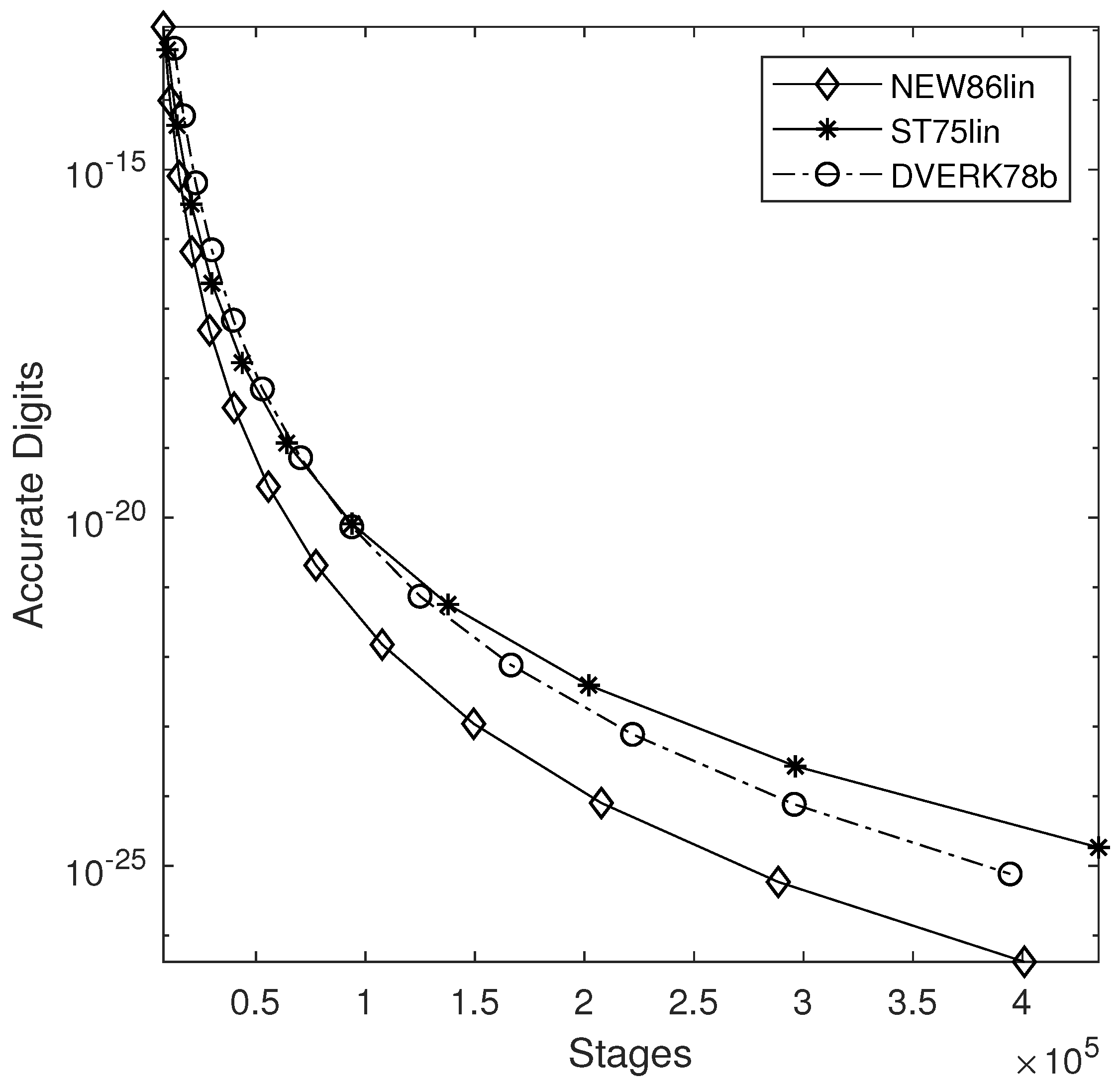
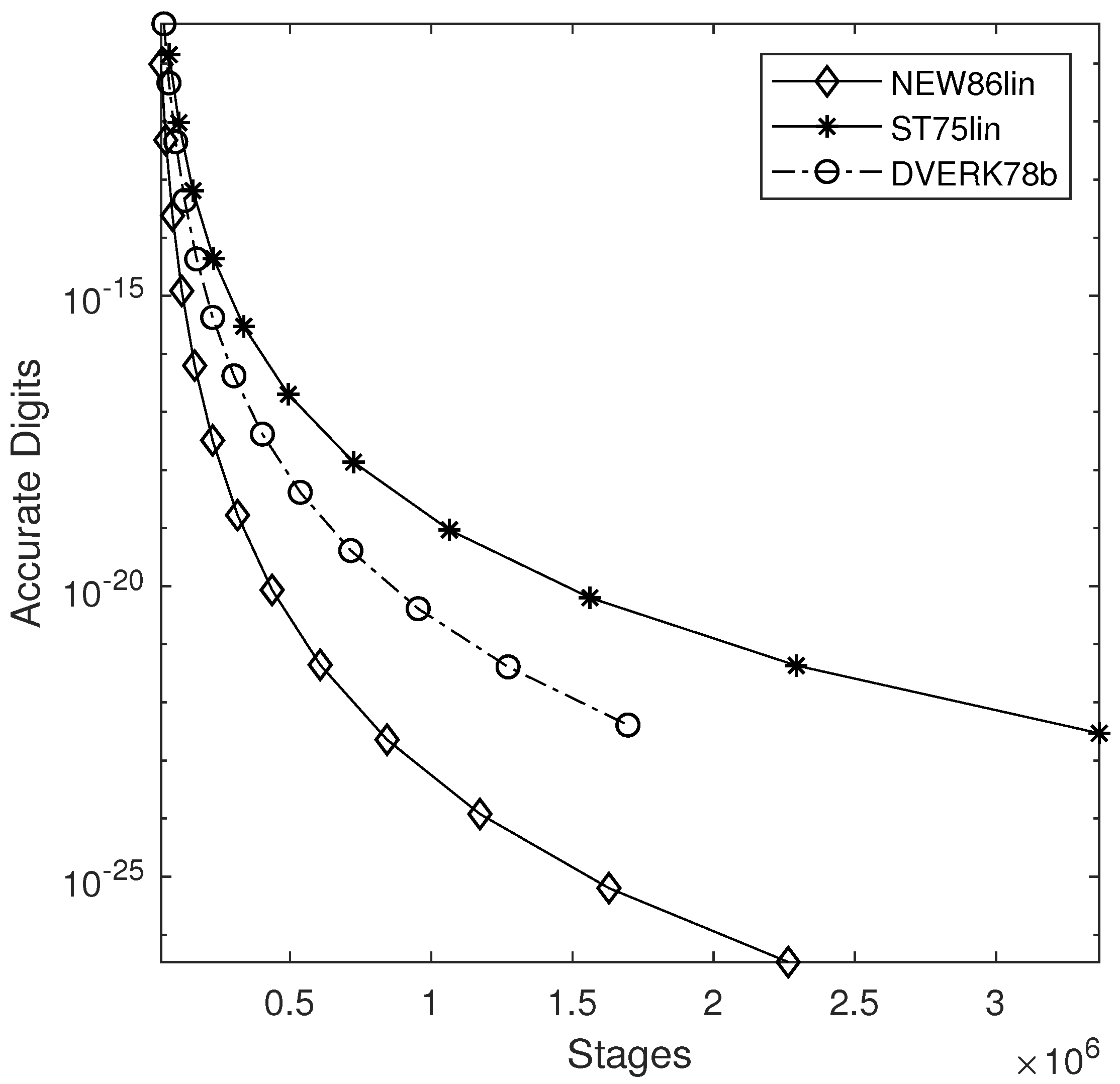
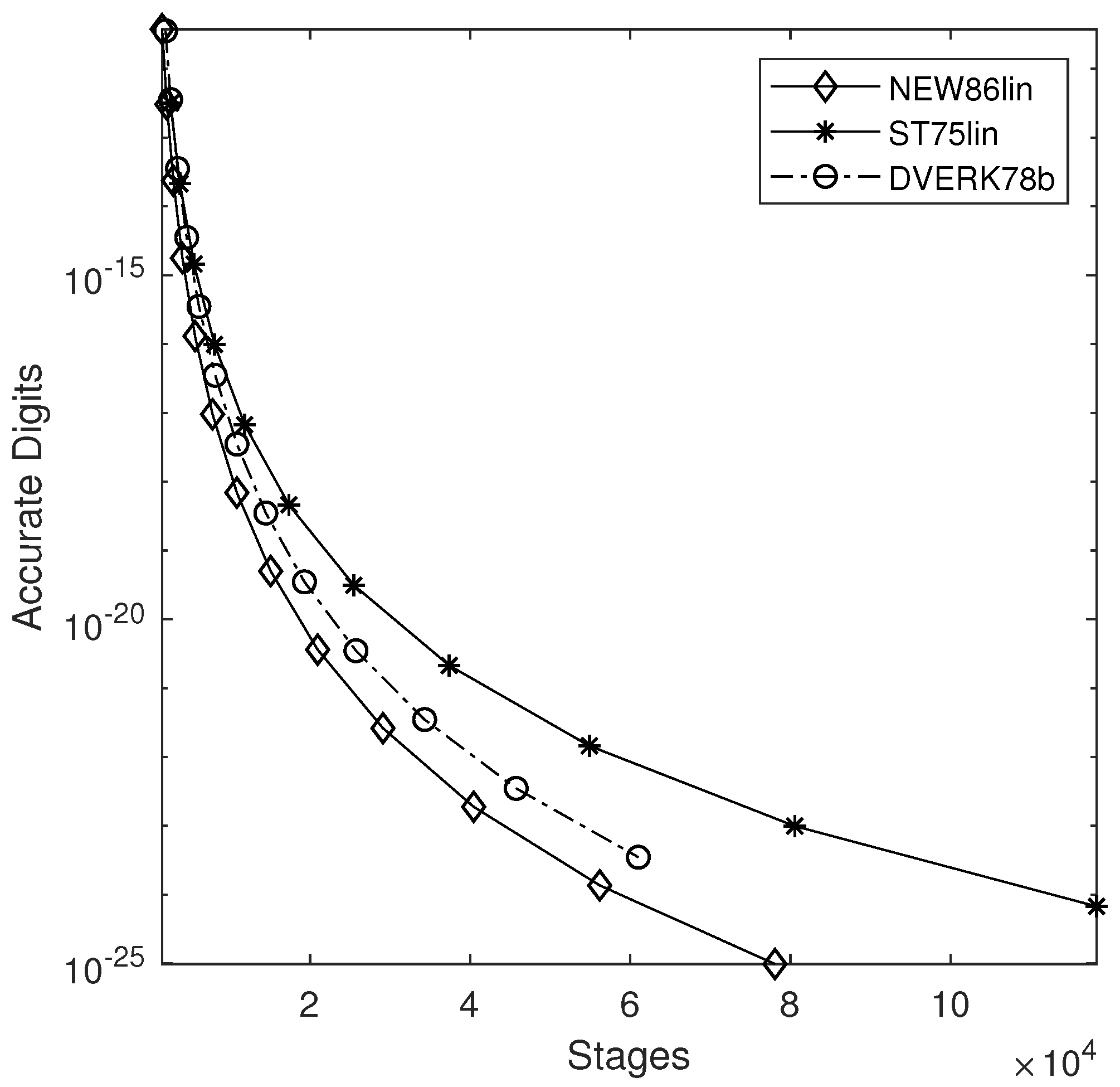
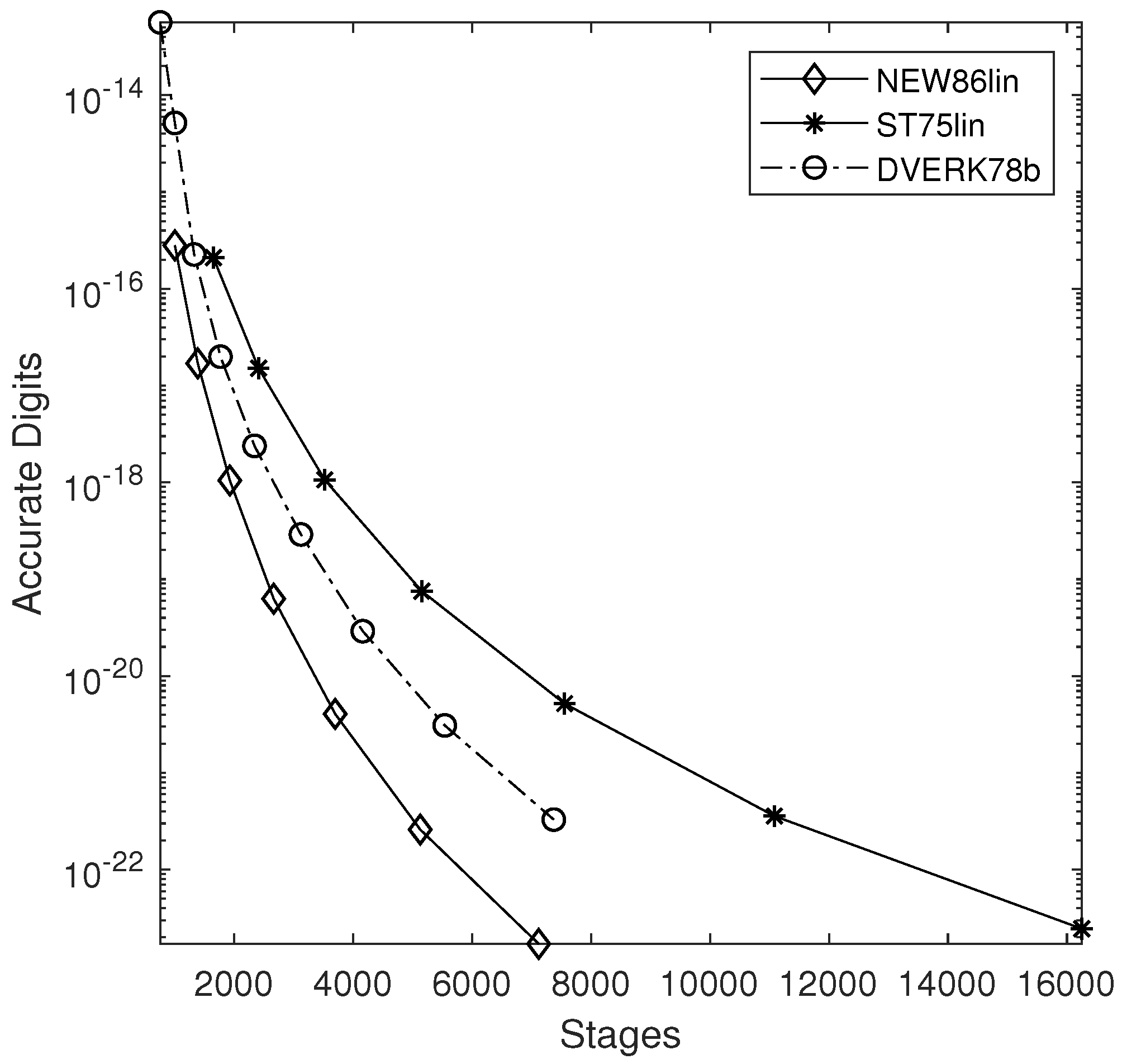
4. Numerical Results

The methods chosen to be compared are the following

• DVERK78b: 13 stages pair of orders $8\left(7\right)$ proposed in [26].
• ST7(5)lin: Effectively eight stages FSAL pair given in [12] for problems of the form (2).
• NEW8(6)lin: Effectively 10 stages FSAL pair given in Table 3.

The selection of DVERK78b [27] is justified as the dominant eighth-order Runge–Kutta pair commonly used for higher accuracy computations. It is implemented in Mathematica function NDSolve [24,25]. It is also builtin function ode78 for MATLAB [28,29]. On the other hand, ST7(5)lin is the highest order Runge–Kutta pair, especially constructed for addressing problems of the form (2).

The problems are as follows

1. 

Scalar

• Equation:

$$y^{\prime }\left(x\right)=-10y\left(x\right)+cos\left(x\right)$$

• Initial values: $y\left(0\right)=1$
• Interval of integration: $x\in [0,10\pi ]$
• Exact Solution:

$$y\left(x\right)={\displaystyle \frac{91e^{-10x}}{101}}+{\displaystyle \frac{sin\left(x\right)}{101}}+{\displaystyle \frac{10cos\left(x\right)}{101}}$$

All pairs were run for tolerances ${10}^{-12},{10}^{-13},\cdots ,{10}^{-24}$. We recorded the error over the end-points in a logarithmic scale (i.e., the accurate digits observed) and the stages used, including the stages from the rejected steps. The results are given in Figure 1.

2. 

Linear Inhomogeneous

• Equation:

$$y^{″}\left(x\right)=-100y\left(x\right)+99sin\left(x\right)$$

• Initial values: $y\left(0\right)=1,y^{\prime }\left(0\right)=11$
• Interval of integration: $x\in [0,20\pi ]$
• Exact solution:

$$y\left(x\right)=cos\left(10x\right)+sin\left(10x\right)+sin\left(x\right)$$

All of the pairs were again run for the same tolerances under the same conditions. The results are presented in Figure 2.

3. 

Simple system

• Equation:

$$\left[\begin{array}{c}{y}_1^{\prime }\\ y_2^{\prime }\end{array}\right]=\left[\begin{array}{cc}-1& 2\\ 2& -4\end{array}\right]·\left[\begin{array}{c}{y}_1\\ y_2\end{array}\right]+\left[\begin{array}{c}sinx\\ -cosx\end{array}\right]$$

• Initial values: $y\left(0\right)={[1,1]}^T$
• Interval of integration: $y\in [0,10\pi ]$
• Exact solution:

$$\left[\begin{array}{c}{y}_1\left(x\right)\\ y_2\left(x\right)\end{array}\right]=\left[\begin{array}{c}2-7/26·exp(-5x)-19/26·cosx-9/26·sinx\\ 1+7/13·exp(-5x))-7/13·cosx-4/13·sinx\end{array}\right]$$

All the pairs were run again for the same tolerances under the same concept. The results are presented in Figure 3.

4. 

Vibratory system

• Equation:

$$\left[\begin{array}{cc}{m}_1& 0\\ 0& m_2\end{array}\right]\left[\begin{array}{c}{y}_1^{″}\\ y_2^{″}\end{array}\right]+\left[\begin{array}{cc}{c}_1+c_2& -c_2\\ -c_2& c_2\end{array}\right]\left[\begin{array}{c}{y}_1^{\prime }\\ y_2^{\prime }\end{array}\right]+\left[\begin{array}{cc}{k}_1+k_2& -k_2\\ -k_2& k_2\end{array}\right]\left[\begin{array}{c}{x}_1\\ x_2\end{array}\right]=\left[\begin{array}{c}{F}_1\left(t\right)\\ 0\end{array}\right],$$

with

$$m_1=1,m_2=2,k_1=1,k_2=10,c_1={\displaystyle \frac{1}{10}},c_2={\displaystyle \frac{1}{5}},F_1\left(t\right)=cos\left(2\pi x\right),$$

• as described in [30].
• Initial values: $y\left(0\right)={[1,0]}^T$, $y^{\prime }\left(0\right)={[0,0]}^T$
• Interval of integration: $x\in [0,2\pi ]$
• Exact solution at the end point (found by a very accurate integration at tolerance ${10}^{-40}$ using Mathematica):
  • $y_1\left(2\pi \right)=-0.04764758829065460843896345564788785624006780,$
  • $y_2\left(2\pi \right)=-0.39560738123536577456428098690215765846542091,$
  • $y_1^{\prime }\left(2\pi \right)=0.5077526053298361513695705553312608275326180,$
  • $y_2^{\prime }\left(2\pi \right)=-0.0975847464163963171387329282131464674805176$

The results for this problem are presented in Figure 4.

5. 

Larger system

• Equation:

$$y^{\prime }=\left[\begin{array}{ccccc}-3& 1& 0& 0& 0\\ 0& -5& 1& 1& 0\\ 1& 0& -5& -1& 0\\ 0& 1& 0& -6& 1\\ 0& 1& 0& 0& -3\end{array}\right]·y-\left[\begin{array}{c}0\\ 0\\ 0\\ 0\\ sin\left(5x\right)\end{array}\right]$$

• Initial values: $y\left(0\right)={[1,0,-1,2,0]}^T$
• Interval of integration: $x\in [0,2]$
• Exact solution at the end point (found by a very accurate integration at tolerance ${10}^{-40}$ using Mathematica):
  • $y_1\left(2\right)=0.00292327770545109146498478585606418,$
  • $y_2\left(2\right)=-0.00216214365051708782733635811791073,$
  • $y_3\left(2\right)=0.00416109102906245143875962662918850,$
  • $y_4\left(2\right)=-0.0200426862728389357033306132363368,$
  • $y_5\left(2\right)=-0.0753110060476118732285104577724070$

The results for this problem are presented in Figure 5. The rightmost lower entries for NEW86lin and DVERK78b in that figure were achieved with Mathematica 13.3, at about the same time of 0.25 s in an AMD Ryzen 9 3900X Processor (Advanced Micro Devices, Inc., Santa Clara, CA, USA) running at 3.79 GHz. Actually, the new method used 7119 stages attaining $22.8$ digits, while DVERK78b used 7373 stages and achieved only $21.5$ accurate digits.

Interpreting the results, we observe a clear and wide distance in favor of NEW86lin. Especially in the inhomogeneous equation, it takes advantage of its high phase-lag accuracy and furnishes much more digits of accuracy than the others.

We may reproduce thereported results using the coefficients listed above. Thus, writing:

• In[6]:= Needs[“DifferentialEquations‘NDSolveProblems’”];
•      Needs[“DifferentialEquations‘NDSolveUtilities’”];
• In[8]:= T86={“ExplicitRungeKutta”,“Coefficients”->T86Coefficients,
•         “DifferenceOrder”->8,“StiffnessTest”->False};
• In[9]:= system=NDSolveProblem[{{y’[t]==-10*y[t]+Cos[t]},{y[0]==1},
•          {y[t]},{t,0,10*Pi},{},{},{}}];
•      refsol={10/101};
•      CompareMethods[system,refsol,{T86},WorkingPrecision->33,
•                  AccuracyGoal->22,PrecisionGoal->22]
• Out[11]= {{{36439,4},400875,4.170180*10^-27}}

We conclude that for problem-1, around 400,000 function evaluations are needed for NEW86lin to furnish $26.4$ digits of accuracy. This is noted as the rightmost lower diamond in Figure 1.

5. Conclusions

This study focuses on the application of Runge–Kutta methods to linear inhomogeneous problems. The algebraic order conditions are systematically presented, leveraging their association with rooted trees. A specific 8(6)-order pair is derived using evolutionary optimization strategies. The effectiveness of this approach is demonstrated through its application to a range of pertinent problems.

References

1. Kovalnogov, V.N.; Fedorov, R.V.; Karpukhina, T.V.; Evgenievich, C.Y.; Simos, T.E.; Tsitouras, C. An Algorithmic approach to Runge–Kutta–Nystrom pairs. TWMS J. Pure Appl. Math. 2023, 14, 3–22. [Google Scholar]
2. Li, R.; Lin, R.-L.; Simos, T.E.; Tsitouras, C. A novel approach on high order Runge-Kutta-Nystrom error estimators. Appl. Comput. Math. 2023, 22, 246–258. [Google Scholar]
3. Simos, T.E.; Tsitouras, C.; Famelis, I.T. Explicit Numerov Type Methods with Constant Coefficients: A Review. Appl. Comput. Math. 2017, 16, 89–113. [Google Scholar]
4. Simos, T.E.; Tsitouras, C. High phase–lag order, four–step methods for solving y″ = f(x,y). Appl. Comput. Math. 2018, 17, 307–316. [Google Scholar]
5. Shampine, L.F. Cheaper integration of linear systems. Simulation 1973, 20, 17. [Google Scholar] [CrossRef]
6. England, R. Error estimates for Runge–Kutta type solutions of systems of ordinary differential equations. Comput. J. 1969, 12, 166–170. [Google Scholar] [CrossRef]
7. Enright, W.H. The efficient solution of linear constant-coefficient systems of differential equations. Simulation 1978, 30, 129–133. [Google Scholar] [CrossRef]
8. Zingg, D.W.; Chisholm, T.T. Runge-Kutta methods for linear ordinary differential equations. Appl. Numer. Math. 1999, 31, 227–238. [Google Scholar] [CrossRef]
9. Butcher, J.C. Implicit Runge-Kutta processes. Math. Comput. 1964, 18, 50–64. [Google Scholar]
10. Butcher, J.C. On Runge-Kutta processes of high order. J. Austral. Math. Soc. 1964, 4, 179–194. [Google Scholar] [CrossRef]
11. Tsitouras, C.; Papakostas, S.N. Cheap error estimation for Runge-Kutta methods. SIAM J. Sci. Comput. 1999, 20, 2067–2088. [Google Scholar] [CrossRef]
12. Simos, T.E.; Tsitouras, C. Evolutionary derivation of Runge-Kutta pairs for addressing inhomogeneous linear problems. Numer. Algor. 2021, 21, 511–525. [Google Scholar] [CrossRef]
13. Lambert, J.D. Numerical Methods for ODEs; Wiley: Chichester, UK, 1991. [Google Scholar]
14. Butcher, J.C. The Numerical Analysis of ODEs: Runge-Kutta and General Linear Methods; Wiley: Chichester, UK, 1987. [Google Scholar]
15. Hairer, E.; Nørsett, S.P.; Wanner, G. Solving Ordinary Differential Equations I; Springer: Berlin/Heidelberg, Germany, 1987. [Google Scholar]
16. Fehlberg, E. Low Order Classical Runge-Kutta Formulas with Step-Size Control and Their Application to Some Heat Transfer Problems; NASA Tech. Rep. TR R-315; NASA Marshall Space Flight Center: Huntsville, AL, USA, 1969.
17. Shampine, L.F. Some practical Runge–Kutta formulas. Math. Comput. 1986, 46, 135–150. [Google Scholar]
18. Houwen, P.J.V.D.; Sommeijer, B.P. Explicit Runge-Kutta-Nyström methods with reduced phase errors for computing oscillating solutions. SIAM J. Numer. Anal. 1987, 24, 595–617. [Google Scholar] [CrossRef]
19. Chawla, M.M.; Rao, P.S. An explicit sixth-order method with phase-iag of order eight for y″ = f(x,y). J. Comput. Appl. Math. 1987, 17, 365–368. [Google Scholar]
20. Storn, R.; Price, K. Differential evolution—A simple and efficient heuristic for global optimization over continuous spaces. J. Glob. Optim. 1997, 11, 341–359. [Google Scholar] [CrossRef]
21. Price, K.; Storn, R.M.; Lampinen, J.A. Differential Evolution: A Practical Approach to Global Optimization; Springer: Berlin/Heidelberg, Germany, 2006; ISBN 978-3-540-20950-8. [Google Scholar]
22. Feoktistov, V. Differential Evolution: In Search of Solutions; Springer: Berlin/Heidelberg, Germany, 2006; ISBN 978-0-387-36895-5. [Google Scholar]
23. Wolfram Research, Inc. Mathematica, Version 11.3.0; Wolfram Research, Inc.: Champaign, IL, USA, 2018. [Google Scholar]
24. NDSolve: Mathematica Function. Available online: https://reference.wolfram.com/language/ref/NDSolve.html?q=NDSolve (accessed on 17 March 2025).
25. “ExplicitRungeKutta” for NDSolve. Available online: https://reference.wolfram.com/language/tutorial/NDSolveExplicitRungeKutta.html (accessed on 17 March 2025).
26. Verner, J.H. Available online: https://www.sfu.ca/~jverner/RKV87.IIa.Robust.00000754677.081208.FLOAT40OnWeb (accessed on 17 March 2025).
27. Verner, J.H. Numerically optimal Runge–Kutta pairs with interpolants. Numer. Algor. 2010, 53, 383–396. [Google Scholar] [CrossRef]
28. MATLAB, version R2019b; The Mathworks, Inc.: Natick, MA, USA, 2019.
29. ode78: Matlab Function. Available online: https://www.mathworks.com/help/matlab/ref/ode78.html (accessed on 17 March 2025).
30. Low, K.H. Displacement and Frequency analyses of vibratory systems. Comput. Struct. 1995, 54, 743–755. [Google Scholar] [CrossRef]
Figure 1. Performances on scalar problem.
Axioms 14 00245 g001
Figure 2. Performances on an inhomogeneous equation.
Axioms 14 00245 g002
Figure 3. Performances on a simple system.
Axioms 14 00245 g003
Figure 4. Performances on a vibrator.
Axioms 14 00245 g004
Figure 5. Performances on a larger system.
Axioms 14 00245 g005