A Penalized Profile Quasi-Likelihood Method for a Semiparametric Varying Coefficient Spatial Autoregressive Panel Model with Fixed Effects

Abstract

This paper proposes a variable selection method for a semiparametric varying coefficient spatial autoregressive panel model with fixed effects based on a penalized profile quasi-likelihood method, which can simultaneously select significant variables in parametric components and nonparametric components without estimating fixed effects. With an appropriate selection of the tuning parameters and some mild assumptions, the consistency of this procedure and the oracle property of the obtained estimators are established. Then, we conduct some Monte Carlo simulations to assess the finite sample performance of the proposed variable selection method, and finally, we analyze a real dataset for further illustration.

1. Introduction

Recently, there has been a surge in focus on spatial panel data model research. These models not only account for the spatial interdependencies of economic phenomena but also allow investigators to manage the unobservable heterogeneity among geographical units [1,2,3,4,5]. The basic spatial panel model is specified as follows:

$$y_{it}={\rho }_0\sum _{j=1}^N{w}_{ij}{y}_{jt}+{\mathit{X}}_{it}^{\tau }{\mathit{\beta }}_0+{\mu }_{0i}+{ϵ}_{it}, i=1,2,\dots ,N; t=1,2,\dots ,T,$$

(1)

where $\{y_{it},{\mathit{X}}_{it}\}$ represents the observations of an individual i in period t, $w_{ij}$ denotes the spatial weight between an individual i and j, ${\mu }_{0i}$ denotes the unobserved and time-invariant individual effect, ${ϵ}_{it}$ denotes random disturbance, and $\{{\rho }_0,{\mathit{\beta }}_0\}$ denotes the unknown true parameter value. However, model (1) adopts a linear specification and conducting parametric statistical inference inherently requires a set of model assumptions, with linearity serving as one of the most practical options. Despite their robust theoretical foundations, linear models frequently fall short in practical applications. Furthermore, when a linear model is misspecified with respect to the data analysis process, it may result in significant modeling biases and misleading conclusions. Therefore, more flexible spatial panel models are required. Ai and Zhang [6] extended model (1) to a partially linear spatial panel model with fixed effects by adding an unknown function, and they proposed a sieve two-stage least squares regression to consistently estimate their model. Zhang and Sun [7] considered a partially specified dynamic spatial panel model, which takes into account past information of the dependent variable. Furthermore, a model known as the semiparametric varying coefficient spatial autoregressive (hereafter, SVCSAR) panel model, which strikes a balance between flexibility and interpretability, is being popularly studied; see [8,9] for more details. The model is specified as follows:

$$y_{it}={\rho }_0\sum _{j=1}^N{w}_{ij}{y}_{jt}+{\mathit{X}}_{it}^{\tau }{\mathit{\beta }}_0+{\mathit{Z}}_{it}^{\tau }{\mathit{\alpha }}_0(u_{it})+{\mu }_{0i}+{ϵ}_{it},i=1,2,\dots ,N;t=1,2,\dots ,T,$$

(2)

where $\{y_{it},u_{it},{\mathit{X}}_{it},{\mathit{Z}}_{it}\}$ represents the observations of an individual i in period t. ${\mathit{\alpha }}_0(u)$ is a vector of unknown functions. Model (2) is a general model that can be reduced to some existing panel models. For instance, if ${\rho }_0=0$, this model is reduced to the varying coefficient panel model studied by [10,11,12,13]. If ${\rho }_0=0$ and ${\mathit{\beta }}_0=\mathbf{0}$, this model is reduced to a varying coefficient panel model [14]. If ${\mathit{\alpha }}_0(·)\equiv \mathbf{0}$, this model generalizes the spatial autoregressive panel model [5]. Moreover, if ${\rho }_0=0$, ${\mathit{\beta }}_0=\mathbf{0}$ and ${\mathit{\alpha }}_0(·)\equiv \mathbf{0}$, this model becomes the classical panel model. However, while model (2) can be reduced to various panel models, it also increases the risk of model misspecification in practical applications. Specifying the model form becomes an inevitable issue, which is equivalent to detecting the zero components of $\{{\rho }_0,{\mathit{\beta }}_0,{\mathit{\alpha }}_0(·)\}$. In other words, a variable selection method for model (2) is required. Additionally, when the number of covariates in model (2) is large, selecting important variables is also a purpose of the variable selection method.

Variable selection constitutes a crucial aspect of contemporary statistical inference. Over the years, numerous variable selection techniques have emerged for parametric models. LASSO [15], SCAD [16], and ALASSO [17] are the most popular methods among them. Based on those methods, variable selection methods for nonparametric or semiparametric models have been established in recent years. Wang et al. [18] considered variable selection for varying coefficient models using the SCAD penalty. Li and Liang [19] utilized the SCAD penalty to identify significant variables within the parametric components of a semiparametric varying coefficient partially linear model. Wang et al. [20] and Zhao and Xue [21] presented a variable selection procedure by combining basis function approximations with SCAD penalty for semiparametric varying coefficient partially linear models. The proposed procedure simultaneously selects significant variables in parametric components and nonparametric components. Tian et al. [22] introduced a novel method for variable selection, which integrates basis function approximations with quadratic inference functions. This approach enables the simultaneous identification of significant variables in both parametric and nonparametric components. For further development of the variable selection methods for nonparametric or semiparametric models, see [23,24,25,26], among others. However, there are few studies on the variable selection of panel model (2), in which spatial components and nonparametric components are simultaneously included.

In this paper, we propose a variable selection procedure for model (2). In order to avoid incidental parameter problems [27] brought by unknown fixed effects, this variable selection procedure combines a profile quasi-likelihood method with the basis function approximation and SCAD penalty to achieve estimation and variable selection simultaneously. The proposed procedure can shrink the spatial, linear, and functional coefficients of irrelevant covariates automatically to achieve variable selection. Moreover, by selecting appropriate tuning parameters, we demonstrate the consistency of our variable selection method. The regression coefficient estimators exhibit the oracle property, which implies that the nonparametric component estimators converge optimally, while the parametric component estimators share the same asymptotic behavior as those derived from the true submodel. This suggests that our penalized estimators perform as effectively as if the true zero coefficients were known. Compared with Liu et al. [28] and Xie et al. [29], we consider panel data and varying coefficient components. In comparison, although Luo and Wu [30] took into account variable selection for the SVCSAR model, the model they analyzed was confined to cross-sectional data. Furthermore, they only selected parametric coefficients. However, our method enables the simultaneous selection of significant variables in both parametric and nonparametric components under panel data.

The rest of this paper is structured as follows. In Section 2, we introduce a variable selection process designed for the SVCSAR panel model with fixed effects. In Section 3, we establish the asymptotic properties of the resulting estimators. In Section 4, we detail the computational steps for obtaining these estimators and discuss the selection of tuning parameters. In Section 5, we conduct simulations to assess the performance of our method with finite samples. Additionally, in Section 6, we provide a real-data analysis to further demonstrate the application of our proposed methodology. Finally, in Section 7, we conclude the article with a concise discussion. All technical proofs supporting the asymptotic results are included in the Appendix A.

2. Penalized Profile Quasi-Likelihood Method

We first consider the SVCSAR panel model described in (2). Specifically, $y_{it}$ and $u_{it}$ are scalars, while ${\mathit{X}}_{it}$ is a $p\times 1$ vector and ${\mathit{Z}}_{it}$ is a $q\times 1$ vector, respectively; ${\mathit{\beta }}_0={({\beta }_{01},{\beta }_{02},\dots ,{\beta }_{0p})}^{\tau }$ is an unknown vector that reflects the linear effect of ${\mathit{X}}_{it}$ on $y_{it}$, and it is assumed that only a subset of its elements are non-zero. Without loss of generality, we assume that the first s elements specifically are non-zero. ${\mathit{\alpha }}_0(u)\equiv {\left({\alpha }_{01}(u),\dots ,{\alpha }_{0k}(u),\dots ,{\alpha }_{0q}(u)\right)}^{\tau }$ is a vector of unknown functions. Similarly, we assume that the first d function is non-zero. ${ϵ}_{it}$ is an i.i.d. disturbance with zero mean and finite unknown variance ${\sigma }_0^2$; thus, $\{{\sigma }_0^2,{\rho }_0,{\mathit{\beta }}_0,{\mathit{\alpha }}_0,{\mu }_{01},\dots ,{\mu }_{0N}\}$ are unknown components. Next, we show a penalized quasi-likelihood method that can skip the estimation of ${\mu }_{0i}(i=1,\dots ,N)$ and shrink the remaining estimators.

Let $n=N\times T,{\mathit{Y}}_n\equiv {({\mathit{Y}}_1^{\tau },\dots ,{\mathit{Y}}_t^{\tau },\dots ,{\mathit{Y}}_T^{\tau })}^{\tau }$ with ${\mathit{Y}}_t={(y_{1t},\dots ,y_{Nt})}^{\tau };{\mathit{W}}_n\equiv {\mathit{I}}_T\otimes {\mathit{W}}_N$, where “⊗” demotes the Kronecker product symbol and ${\mathit{I}}_T$ denotes a T-dimensional identity matrix; ${\mathit{X}}_n\equiv {({\mathit{X}}_1^{\tau },\dots ,{\mathit{X}}_t^{\tau },\dots ,{\mathit{X}}_T^{\tau })}^{\tau }$ with ${\mathit{X}}_t={({\mathit{X}}_{1t},\dots ,{\mathit{X}}_{Nt})}^{\tau }$; ${\mathit{A}}_0\equiv {({\mathit{A}}_{01}^{\tau },\dots ,{\mathit{A}}_{0t}^{\tau },\dots ,{\mathit{A}}_{0T}^{\tau })}^{\tau }$ with ${\mathit{A}}_{0t}={({\mathit{Z}}_{1t}^{\tau }{\mathit{\alpha }}_0(u_{1t}),\dots ,{\mathit{Z}}_{Nt}^{\tau }{\mathit{\alpha }}_0(u_{Nt}))}^{\tau }$; ${\mathit{V}}_n\equiv ({\mathit{V}}_1^{\tau },\dots ,{\mathit{V}}_t^{\tau },\dots ,$${\mathit{V}}_T^{\tau }{)}^{\tau }$ with ${\mathit{V}}_t={({ϵ}_{1t},\dots ,{ϵ}_{Nt})}^{\tau }$; ${\mathit{\mu }}_0={({\mu }_{01},..,{\mu }_{0N})}^{\tau }$ denotes the fixed effects vector; ${\mathit{D}}_n\equiv {\mathit{\iota }}_T\otimes {\mathit{I}}_N$, where ${\mathit{\iota }}_T$ represents a T-dimensional vector with all 1. Then, the model (2) can be expressed in matrix form:

$${\mathit{Y}}_n={\rho }_0{\mathit{W}}_n{\mathit{Y}}_n+{\mathit{X}}_n{\mathit{\beta }}_0+{\mathit{A}}_0+{\mathit{D}}_n{\mathit{\mu }}_0+{\mathit{V}}_n,$$

(3)

where $E({\mathit{V}}_n)=\mathbf{0},\mathrm{var}({\mathit{V}}_n)={\sigma }_0^2{\mathit{I}}_n$. Thus, the unknown parametric component is $({\sigma }_0^2,{\rho }_0,{\mathit{\beta }}_0,{\mathit{\mu }}_0)$, and the unknown nonparametric component is ${\mathit{\alpha }}_0(u)$.

Let $\mathit{\theta }={({\sigma }^2,\rho ,{\mathit{\beta }}^{\tau })}^{\tau }$, ${\mathit{\theta }}_0={({\sigma }_0^2,{\rho }_0,{\mathit{\beta }}_0^{\tau })}^{\tau }$, and ${\mathit{M}}_n(\rho )={\mathit{I}}_n-\rho {\mathit{W}}_n$ for any $\rho$ and ${\mathit{M}}_n\equiv {\mathit{M}}_n({\rho }_0)$. Subsequently, we suggest optimizing the log-Gaussian quasi-likelihood, following the approach taken by [31,32], and the log-Gaussian quasi-likelihood of (3) is

$$\begin{array}{cc}\hfill ln\tilde{L}(\mathit{\theta },\mathit{\mu },\mathit{\alpha }(u))=& -\frac{n}{2}ln2\pi -\frac{n}{2}ln{\sigma }^2+ln|{\mathit{M}}_n(\rho )|\hfill \\ \hfill & -\frac{1}{2{\sigma }^2}{\left({\mathit{M}}_n(\rho ){\mathit{Y}}_n-{\mathit{X}}_n\mathit{\beta }-\mathit{A}-{\mathit{D}}_n\mathit{\mu }\right)}^{\tau }\left({\mathit{M}}_n(\rho ){\mathit{Y}}_n-{\mathit{X}}_n\mathit{\beta }-\mathit{A}-{\mathit{D}}_n\mathit{\mu }\right),\hfill \end{array}$$

(4)

where $\mathit{A}={\left({\mathit{A}}_1^{\tau },\dots ,{\mathit{A}}_t^{\tau },\dots ,{\mathit{A}}_T^{\tau }\right)}^{\tau }$, ${\mathit{A}}_t={\left[{\mathit{Z}}_{1t}^{\tau }\mathit{\alpha }(u_{1t}),\dots ,{\mathit{Z}}_{Nt}^{\tau }\mathit{\alpha }(u_{Nt})\right]}^{\tau }$, and $\mathit{\alpha }(u)={\left[{\alpha }_1(u),\dots ,{\alpha }_q(u)\right]}^{\tau }$. When maximizing Equation (4), we encounter two main challenges: (i) Directly estimating ${\mathit{\mu }}_0$ can lead to the incidental parameter problem [27], especially when ${\mathit{\mu }}_0$ becomes high-dimensional as N increases. (ii) Estimating ${\mathit{\alpha }}_0$ is difficult due to its infinite dimensionality. To address these issues, we follow the approach in Tian et al. [32] and let

$$\mathit{B}(u)={\left(B_1(u),B_2(u),\dots ,B_{K_n+l+1}(u)\right)}^{\tau }$$

denote a vector comprising normalized B-spline basis functions of order l with $K_n$ internal knots. Subsequently, we approximate ${\alpha }_{0k}(u)$ as a linear combination of $B_1(u),B_2(u),\dots ,B_{K_n+l+1}(u)$, i.e., ${\alpha }_{0k}(u)\approx {\mathit{B}}^{\tau }(u){\mathit{\gamma }}_{0k}$ for $k=1,2,\dots ,q$. Consequently, mode (3) can be written as follows:

$${\mathit{Y}}_n\approx {\rho }_0{\mathit{W}}_n{\mathit{Y}}_n+{\mathit{X}}_n{\mathit{\beta }}_0+{\mathit{S}}_n{\mathit{\gamma }}_0+{\mathit{D}}_n{\mathit{\mu }}_0+{\mathit{V}}_n,$$

(5)

where ${\mathit{S}}_n={({\mathit{S}}_1^{\tau },\dots ,{\mathit{S}}_t^{\tau },\dots ,{\mathit{S}}_T^{\tau })}^{\tau }$, ${\mathit{S}}_t=\left[\left({\mathit{I}}_q\otimes \mathit{B}(u_{1t})\right){\mathit{Z}}_{1t},\dots ,\left({\mathit{I}}_q\otimes \mathit{B}(u_{Nt})\right){\mathit{Z}}_{Nt}\right]$, and ${\mathit{\gamma }}_0={({\mathit{\gamma }}_{01}^{\tau },\dots ,{\mathit{\gamma }}_{0q}^{\tau })}^{\tau }$. The log-Gaussian quasi-likelihood of (5) is

$$\begin{array}{cc}\hfill ln\widehat{L}(\mathit{\theta },\mathit{\mu },\mathit{\gamma })=& -\frac{n}{2}ln2\pi -\frac{n}{2}ln{\sigma }^2+ln|{\mathit{M}}_n(\rho )|\hfill \\ \hfill & -\frac{1}{2{\sigma }^2}{\left({\mathit{M}}_n(\rho ){\mathit{Y}}_n-{\mathit{X}}_n\mathit{\beta }-{\mathit{S}}_n\mathit{\gamma }-{\mathit{D}}_n\mathit{\mu }\right)}^{\tau }\left({\mathit{M}}_n(\rho ){\mathit{Y}}_n-{\mathit{X}}_n\mathit{\beta }-{\mathit{S}}_n\mathit{\gamma }-{\mathit{D}}_n\mathit{\mu }\right).\hfill \end{array}$$

(6)

To avoid the incidental parameter problem [27] caused by $\mathit{\mu }$, we first concentrate $\mathit{\mu }$ out and obtain the profile quasi-likelihood. Let $\mathit{\eta }={({\mathit{\theta }}^{\tau },{\mathit{\gamma }}^{\tau })}^{\tau }$. For given $\mathit{\eta }$, from (6), we derive

$$\widehat{\mathit{\mu }}(\mathit{\eta })={({\mathit{D}}_n^{\tau }{\mathit{D}}_n)}^{-1}{\mathit{D}}_n^{\tau }({\mathit{M}}_n(\rho ){\mathit{Y}}_n-{\mathit{X}}_n\mathit{\beta }-{\mathit{S}}_n\mathit{\gamma })$$

and substitute this into (6). Then,

$$\begin{array}{cc}\hfill ln{L}_n(\mathit{\eta })=& -\frac{n}{2}ln2\pi -\frac{n}{2}ln{\sigma }^2+ln|{\mathit{M}}_n(\rho )|\hfill \\ \hfill & -\frac{1}{2{\sigma }^2}{\left({\mathit{M}}_n(\rho ){\mathit{Y}}_n-{\mathit{X}}_n\mathit{\beta }-{\mathit{S}}_n\mathit{\gamma }\right)}^{\tau }{\mathit{J}}_n\left({\mathit{M}}_n(\rho ){\mathit{Y}}_n-{\mathit{X}}_n\mathit{\beta }-{\mathit{S}}_n\mathit{\gamma }\right),\hfill \end{array}$$

(7)

where ${\mathit{J}}_n={({\mathit{I}}_n-{\mathit{Q}}_n)}^{\tau }({\mathit{I}}_n-{\mathit{Q}}_n)$ and ${\mathit{Q}}_n={\mathit{D}}_n{({\mathit{D}}_n^{\tau }{\mathit{D}}_n)}^{-1}{\mathit{D}}_n^{\tau }$.

Inspired by the concept of variable selection in semiparametric varying coefficient partially linear models [21], we introduce a penalized profile quasi-likelihood function defined as follows:

$$Q_n(\mathit{\eta })=ln{L}_n(\mathit{\eta })-n\sum _{j=2}^{p+2}{p}_{{\lambda }_{1,n}}(|{\theta }_j|)-n\sum _{k=1}^q{p}_{{\lambda }_{2,n}}(\parallel {\mathit{B}}^{\tau }(·){\mathit{\gamma }}_k\parallel ),$$

(8)

where $\parallel {\mathit{B}}^{\tau }(·){\mathit{\gamma }}_k\parallel ={(\int {({\mathit{B}}^{\tau }(u){\mathit{\gamma }}_k)}^{2}du)}^{1/2}$, and $p_{\lambda }(·)$ is a SCAD penalty function [16] defined by

$$p_{\lambda }^{\prime }(\omega )=\lambda \left\{I(\omega \le \lambda )+\frac{{(a\lambda -\omega )}_{+}}{(a-1)\lambda }I(\omega \ge \lambda )\right\},$$

with $a>2,\omega >0$ and $p_{\lambda }(0)=0$. Throughout this paper, we adopt the suggestion by Fan and Li [16] that the choice of $a=3.7$ performs well in a variety of situations. The tuning parameter $\lambda$ can be different for all ${\theta }_j$ and ${\mathit{B}}^{\tau }(·){\mathit{\gamma }}_k$. Note that $\parallel {\mathit{B}}^{\tau }(·){\mathit{\gamma }}_k\parallel ={(\int {({\mathit{B}}^{\tau }(u){\mathit{\gamma }}_k)}^{2}du)}^{1/2}={({\mathit{\gamma }}_k^{\tau }\mathit{H}{\mathit{\gamma }}_k)}^{1/2}\equiv {\parallel {\mathit{\gamma }}_k\parallel }_{\mathit{H}}$, where $\mathit{H}=\int \mathit{B}(u){\mathit{B}}^{\tau }(u)du$. Then, the penalized profile quasi-likelihood function can be written as follows:

$$Q_n(\mathit{\eta })=ln{L}_n(\mathit{\eta })-n\sum _{j=2}^{p+2}{p}_{{\lambda }_{1,n}}(|{\theta }_j|)-n\sum _{k=1}^q{p}_{{\lambda }_{2,n}}(\parallel {\mathit{\gamma }}_k{\parallel }_{\mathit{H}}).$$

(9)

Let $\widehat{\mathit{\eta }}={({\widehat{\mathit{\theta }}}^{\tau },{\widehat{\mathit{\gamma }}}^{\tau })}^{\tau }$ be the solution by maximizing (9). Then, $\widehat{\mathit{\theta }}$ is the penalized profile quasi-likelihood estimator (penalized profile QMLE) of $\mathit{\theta }$, and the estimator of ${\alpha }_k(u)$ can be obtained by ${\alpha }_k(u)={\mathit{B}}^{\tau }(u){\widehat{\mathit{\gamma }}}_k$. Next, we study the asymptotic properties of the resulting penalized profile likelihood estimators. Without loss of generality, we assume that ${\theta }_{0j}=0$ for $j=s+1,\dots ,p+2$, with the remaining ${\theta }_{0j}(j=1,\dots ,s)$ being the non-zero components of ${\mathit{\theta }}_0$. Similarly, we assume that ${\alpha }_{0k}(·)\equiv 0$ for $k=d+1,\dots ,q$ and that the ${\alpha }_{0k}(·),(k=1,\dots ,d)$ constitute all the non-zero components of ${\mathit{\alpha }}_0(·)$.

3. Asymptotic Results

Denote ${\mathit{G}}_n={\mathit{W}}_n{\mathit{M}}_n^{-1}$, ${\mathit{R}}_n={\mathit{G}}_n({\mathit{X}}_n{\mathit{\beta }}_0+{\mathit{A}}_0+{\mathit{D}}_n{\mathit{\mu }}_0)$. The following assumptions are necessary prior to establishing the asymptotic properties.

C1

T is finite and greater than 2, and N is large.

C2

The disturbances $\{{ϵ}_{it}\}$ for $i=1,2,\dots ,n$ and $t=1,2,\dots ,T$ are independently and identically distributed with zero mean, and the finite variance is ${\sigma }_0^2$. Additionally, for some $v>0$, $E|{ϵ}_{it}{|}^{4+v}$ exists.

C3

The entries $\{w_{ij}\}$ of ${\mathit{W}}_n$ satisfy $w_{ii}=0$ and $w_{ij}=O(1/h_n)$, where $h_n/n\to 0$ as $n\to \infty$.

C4

The matrix ${\mathit{M}}_n(\rho )$ is nonsingular for all $\rho$ in a compact parameter space $\mathsf{\Lambda }$. The sequences $\{{\mathit{M}}_n^{-1}(\rho )\}$ are uniformly bounded in either row or column sums for all $\rho \in \mathsf{\Lambda }$. The true ${\rho }_0$ is in the interior of $\mathsf{\Lambda }$.

C5

The sequences of matrices $\{{\mathit{W}}_n\}$ and $\{{\mathit{M}}_n^{-1}\}$ are uniformly bounded in both row and column sums.

C6

The elements of ${\mathit{X}}_n$ and ${\mathit{S}}_n$ are uniformly bounded for all n, and the limit ${lim}_{n\to \infty }{n}^{-1}{({\mathit{X}}_n,{\mathit{S}}_n,{\mathit{R}}_n)}^{\tau }{\mathit{J}}_n({\mathit{X}}_n,{\mathit{S}}_n,{\mathit{R}}_n)$ exists and is nonsingular.

C7

There exists a constant ${\lambda }_c$, such that ${\lambda }_c{\mathit{I}}_n-{\mathbf{\Gamma }}_n{\mathbf{\Gamma }}_n^{\tau }$ is positive and semidefinite for all n, where ${\mathbf{\Gamma }}_n={\mathit{R}}_n,{\mathit{X}}_n,{\mathit{G}}_n$.

C8

The limits ${lim}_{n\to \infty }E[n^{-1}{\partial }^{2}ln{L}_n({\mathit{\eta }}_T)/\partial \mathit{\eta }\partial {\mathit{\eta }}^{\tau }]$ exist.

C9

Third derivatives ${\partial }^{3}ln{L}_n(\mathit{\eta })/(\partial {\eta }_i\partial {\eta }_j\partial {\eta }_k)$ exist for all $\mathit{\eta }$ in an open set $\mathbb{H}$ that contains the parameter point ${\mathit{\eta }}_T$. Furthermore, there exist functions $M_{ijk}$, such that $|{\partial }^{3}ln{L}_n(\mathit{\eta })/(\partial {\eta }_i\partial {\eta }_j\partial {\eta }_k)| \le M_{ijk}$ for all $\eta \in \mathbb{H}$, where $E(M_{ijk})\le \infty$ for $i,j,k$.

C10

For $k=1\dots q$, ${\alpha }_k(u)\in C^r(0,1)$, where $r\ge 2$. The distribution of $u_{it}$ is absolutely continuous, and its density is bound away from zero and infinity on $[0,1]$.

C11

Let ${\pi }_1,\dots ,{\pi }_{K_n}$ denote the interior knots within the interval $[0,1]$ and ${\pi }_0=0$, ${\pi }_{K_n+1}=1$. Define ${\varrho }_i={\pi }_i-{\pi }_{i-1}$. There exists a constant C, such that $max{\varrho }_i/min{\varrho }_i\le C$ and $max\{{\varrho }_i\}=o(K_n^{-1})$.

C12

The knot number $K_n$ is assumed to satisfy $K_n=n^{\frac{1}{2r+1}}$.

C13

Let $b_n={max}_{j,k}\{p_{{\lambda }_{1j}}^{″}(|{\theta }_{0j}),p_{{\lambda }_{2,n}}^{″}(\parallel {\mathit{\gamma }}_{0k}{\parallel }_{\mathit{H}}) : |{\theta }_{0j}|\ne 0,\parallel {\mathit{\gamma }}_{0k}{\parallel }_{\mathit{H}}\ne 0\}$. Then, $b_n\to 0$, as $n\to \infty$.

C14

$j=s+1,\dots ,p,k=d+1,\dots ,q$, $lim{inf}_{n\to \infty }lim{inf}_{{\theta }_j\to 0^{+}}{\lambda }_{2j}^{-1}{p}_{{\lambda }_{2j}}^{\prime }(|{\theta }_j|)>0$ and $lim{inf}_{n\to \infty }lim{inf}_{\parallel {\mathit{\gamma }}_{0k}{\parallel }_{\mathit{H}}\to 0^{+}}{\lambda }_{2k}^{-1}{p}_{{\lambda }_{2k}}^{\prime }(\parallel {\mathit{\gamma }}_{0k}{\parallel }_{\mathit{H}})>0$ hold.

Remark 1.

C1 excludes the scene where T approaches infinity. Essentially, this assumption implies a setting (large N, small T) aligning with many spatial data studies. Conversely, the scenarios in which only T increases indefinitely and where both N and T go to infinity closely resemble the scenario where only N goes to infinity. C2 is needed to apply the central limit theorem in Kelejian and Prucha [33]. C3–C5 are analogous to Assumption 2 in Lee [31], which focuses on the properties of the spatial weight matrix ${\mathit{W}}_n$ and is essential for the identifiability of ρ. Specifically, $\mathsf{\Lambda }=(-1,1)$ when ${\mathit{W}}_n$ satisfies ${\sum }_{j=1}^n{w}_{ij}=1$ for all i. C6–C9 are applied for asymptotic normality of the profile QMLE. C10–C12 facilitate achieving the optimal convergence rate for ${\widehat{\alpha }}_k(u)$. He et al. [34] suggested that cubic B-splines are adequate for accurately approximating nonparametric functions, with the number of interior knots set to the integer part of $n^{1/5}$. Meanwhile, C13 and C14 present assumptions about the penalty function, which are comparable to those utilized in [16,18,19].

Due to the projection matrix ${\mathit{J}}_n$, a portion of the degrees of freedom is lost; therefore, the estimator ${\widehat{\sigma }}^2$ derived from (9) is not a consistent estimator of ${\sigma }_0^2$. A correction is needed. Let ${\sigma }_T^2=(T-1){\sigma }_0^2/T,{\mathit{\theta }}_T={({\sigma }_T^2,{\rho }_0,{\mathit{\beta }}_0^{\tau })}^{\tau }$ and ${\mathit{\eta }}_T={({\mathit{\theta }}_T^{\tau },{\mathit{\gamma }}_0^{\tau })}^{\tau }$. Under the assumptions, the subsequent theorem establishes the consistency property of the penalized profile QMLE.

Theorem 1.

Suppose that Assumptions C1–C12 hold; then, we can have

$$\parallel {\widehat{\alpha }}_k(·)-{\alpha }_{0k}(·)\parallel =O_p(n^{-r/(2r+1)}+a_n),k=1,\dots ,q,$$

where $a_n={max}_{j,k}\left\{p_{{\lambda }_{1j}}^{\prime }(|{\theta }_{0j}|),p_{{\lambda }_{2k}}^{\prime }(\parallel {\mathit{\gamma }}_{0k}{\parallel }_{\mathit{H}}) : |{\theta }_{0j}|\ne 0,\parallel {\mathit{\gamma }}_{0k}{\parallel }_{\mathit{H}}\ne 0\right\}.$

Furthermore, under some conditions, we show that such consistent estimators must possess the sparsity property, which is stated as follows.

Theorem 2.

Suppose that Assumptions C1–C14 hold, and let ${\lambda }_{max}={max}_{j,k}\left\{{\lambda }_{1j},{\lambda }_{2k}\right\}$ and ${\lambda }_{min}={min}_{j,k}\left\{{\lambda }_{1j},{\lambda }_{2k}\right\}$. If ${\lambda }_{max}\to 0$ and $n^{r/(2r+1)}{\lambda }_{min}\to \infty$ as $n\to \infty$, then, with probability tending to 1, $\widehat{\mathit{\beta }}$ and $\widehat{\mathit{\alpha }}(·)$ must satisfy

(i) 

${\widehat{\beta }}_j=0, j=s+1,\dots ,p.$

(ii) 

${\widehat{\alpha }}_k(·)\equiv 0, k=d+1,\dots ,q.$

According to Remark 1 in Fan and Li [16], if ${\lambda }_{max}\to 0$ as $n\to \infty$, then $a_n=0$. Consequently, based on Theorems 1 and 2, it becomes evident that by selecting appropriate tuning parameters, our variable selection approach is consistent. Furthermore, the estimators of the nonparametric components attain the optimal convergence rate as if the subset of true zero coefficients were already known [35]. Subsequently, we will demonstrate that the estimators for the non-zero coefficients in the parametric components share the same asymptotic distribution as those derived from the correct submodel. Let ${\widehat{\mathit{\theta }}}^{\ast }={({\widehat{\theta }}_1,\dots ,{\widehat{\theta }}_s)}^{\tau },$ ${\mathit{\theta }}_T^{\ast }={({\theta }_{T1},\dots ,{\theta }_{Ts})}^{\tau }$, where the following result states the asymptotic normality of $\widehat{\mathit{\theta }}$.

Theorem 3.

Suppose that Assumptions C1–C14 and the conditions in Theorem 2 hold, then

$$\sqrt{n}({\widehat{\mathit{\theta }}}^{\ast }-{\mathit{\theta }}_T^{\ast })\to N\left(\mathbf{0},\frac{T}{T-1}\left\{{\mathbf{\Omega }}^{-1}+{\mathbf{\Omega }}^{-1}[{\mathbf{\Psi }}_{\mathit{\theta }}^{\ast }-2{\mathbf{\Sigma }}_{\mathit{\theta }\mathit{\gamma }}^{\ast \tau }{({\mathbf{\Sigma }}_{\mathit{\gamma }}^{\ast })}^{-1}{\mathbf{\Psi }}_{\mathit{\theta }}^{\ast }]{\mathbf{\Omega }}^{-1}\right\}\right),$$

where $\mathbf{\Omega },{\mathbf{\Psi }}_{\mathit{\theta }}^{\ast },{\mathbf{\Sigma }}_{\mathit{\gamma }}^{\ast },{\mathbf{\Sigma }}_{\mathit{\theta }\mathit{\gamma }}^{\ast }$ are defined in the Appendix A.

4. Some Issues in Practice

In the practical situation, we have to choose the proper tuning parameters $({\lambda }_1,{\lambda }_2)$ and provide an effective calculation algorithm. In this section, we discuss these practical issues.

4.1. Selection of Tuning Parameters

The tuning parameters ${\lambda }_{1k}$’s and ${\lambda }_{2k}$’s should be chosen. In practice, we suggest taking ${\lambda }_{1j}={\lambda }_1/|{\beta }_j^{(0)}|$ and ${\lambda }_{2k}={\lambda }_2/{\parallel {\mathit{\gamma }}_k^{(0)}\parallel }_{\mathit{H}}$, and the pair $({\lambda }_1,{\lambda }_2)$ is derived by minimizing the following BIC-type criterion:

$$BIC({\lambda }_1,{\lambda }_2)=-2ln{L}_n({\widehat{\mathit{\eta }}}_{{\lambda }_1,{\lambda }_2})+d{f}_{{\lambda }_1,{\lambda }_2}\times lnn,$$

where ${\widehat{\mathit{\eta }}}_{{\lambda }_1,{\lambda }_2}$ is the $\widehat{\mathit{\eta }}$ derived for given ${\lambda }_1,{\lambda }_2$, and $d{f}_{{\lambda }_1,{\lambda }_2}$ is the number of non-zero elements of both $\widehat{\mathit{\theta }}$ and $(\parallel {\widehat{\mathit{\gamma }}}_1{\parallel }_{\mathit{H}},\dots ,\parallel {\widehat{\mathit{\gamma }}}_q{\parallel }_{\mathit{H}})$.

4.2. Computational Algorithm

Given that $Q_n(\mathit{\eta })$ is not differentiable at the origin, the standard gradient method cannot be employed. Therefore, we have devised an iterative algorithm that relies on a local quadratic approximation of the penalty function $p_{\lambda }(·)$, similar to the approach taken by Fan and Li [16]. Let

$$\left\{\begin{array}{c}\mathit{f}(\mathit{\eta })=\frac{\partial ln{L}_n(\mathit{\eta })}{\partial \mathit{\eta }},\hfill \\ \mathbf{\Gamma }(\mathit{\eta })=\mathrm{diag}\left\{0,\frac{p_{{\lambda }_{12}}^{\prime }(|{\theta }_1|)}{|{\theta }_1|},\dots ,\frac{p_{{\lambda }_{1p}}^{\prime }(|{\theta }_p|)}{|{\theta }_p|},\frac{p_{{\lambda }_{21}}^{\prime }(\parallel {\mathit{\gamma }}_1{\parallel }_{\mathit{H}})}{\parallel {\mathit{\gamma }}_1{\parallel }_{\mathit{H}}}\mathit{H},\dots ,\frac{p_{{\lambda }_{2q}}^{\prime }(\parallel {\mathit{\gamma }}_q{\parallel }_{\mathit{H}})}{\parallel {\mathit{\gamma }}_q{\parallel }_{\mathit{H}}}\mathit{H}\right\},\hfill \\ \mathit{U}(\mathit{\eta })=\mathbf{\Gamma }(\mathit{\eta })\mathit{\eta },\hfill \\ \mathbf{\Sigma }(\mathit{\eta })=\frac{{\partial }^{2}ln{L}_n(\mathit{\eta })}{\partial \mathit{\eta }\partial {\mathit{\eta }}^{\tau }}.\hfill \end{array}\right.$$

Then, a feasible algorithm is as follows:

Step 1

Initialize ${\mathit{\eta }}^{(0)}$.

Step 2

Update ${\mathit{\eta }}^{(m+1)}={\mathit{\eta }}^{(m)}-{[\mathbf{\Sigma }({\mathit{\eta }}^{(m)})+\mathbf{\Gamma }({\mathit{\eta }}^{(m)})]}^{-1}[\mathit{f}({\mathit{\eta }}^{(m)})-\mathit{U}({\mathit{\eta }}^{(m)})]$.

Step 3

Iterate Step 2 until convergence, and denote the final estimators as the penalized profile quasi-likelihood estimators.

The initial value ${\eta }^{(0)}$ in Step 1 is obtained from the profile QMLE, i.e., $\partial ln{L}_n({\mathit{\eta }}^{(0)})/\partial \mathit{\eta }=0$.

5. Monte Carlo Simulations

In this section, we conduct Monte Carlo simulations to assess the finite sample performance of our proposed method. Following the methodology employed by Li and Liang in [19], we evaluate the estimator $\widehat{\mathit{\theta }}$ using the generalized mean square error (GMSE), which is defined as follows:

$$\mathrm{GMSE}=\frac{1}{n}{(\widehat{\mathit{\theta }}-{\mathit{\theta }}_T)}^{\tau }\left[{(\mathbf{1},{\mathit{W}}_n\mathit{Y},\mathit{X})}^{\tau }(\mathbf{1},{\mathit{W}}_n\mathit{Y},\mathit{X})\right](\widehat{\mathit{\theta }}-{\mathit{\theta }}_T).$$

The performance of estimator $\widehat{\mathit{\alpha }}(·)$ is assessed using average square errors (ASE):

$$\mathrm{ASE}=\left\{\frac{1}{S}\sum _{s=1}^S\sum _{k=1}^q{\left[{\widehat{\alpha }}_k(u_s)-{\alpha }_{0k}(u_s)\right]}^2\right\},$$

where $u_s,s=1,\dots ,S$ are the grid points at which the function $\widehat{\mathit{\alpha }}(·)$ is evaluated. In our simulation, $S=200$ is used.

The spatial matrix is generated from the following procedure. (i) Calculate $G_N=\mathrm{round}(N^{0.8})$ as the number of “groups” and $m=N^{0.2}$ as the average number of individuals in each group. (ii) Generate the “group” size $n_i\sim Uniform(0.8m,1.2m)(i=1,\dots ,G_N)$ and adjust $n_i$ so that it satisfies ${\sum }_{i=1}^{G_N}{n}_i=N$. (iii) Normalize the matrices ${\mathit{W}}_i(i=1,\dots ,G_N)$ with zero for diagonal elements and $1/(n_i-1)$ for other elements. (iv) Generate the final spatial matrix ${\mathit{W}}_N=\mathrm{diag}\{{\mathit{W}}_1,\dots ,{\mathit{W}}_{G_N}\}$.

Data are generated from model (2), and we construct two examples to simulate different scenarios. Example 1 is a regular example that is primarily used to verify the asymptotic properties of penalized profile likelihood estimators. Various sample sizes, degrees of spatial dependence, distributions of disturbances, and variances in disturbances are considered. Example 2 focuses on examining the performance of the proposed method in cases where the sample size is large, and the dimensions of parametric and nonparametric components are high. Unlike Example 1, Example 2 includes covariates with AR structure and different functions. All simulation results are obtained based on 500 repetitions.

5.1. Example 1: Regular Scenario

Let ${\mathit{\beta }}_0={(2,-1,{\mathbf{0}}_5)}^{\tau }$, ${\mathit{\alpha }}_0(u)={(2sin(2\pi u),2cos(2\pi u),{\mathbf{0}}_5)}^{\tau }$. To simulate different spatial degrees, we choose different ${\rho }_0\in \{0,0.3,0.7\}$. We take two distribution settings for ${\epsilon }_{it}$: (i) ${\epsilon }_{it}\sim N(0,{\sigma }_0^2)$ and (ii) ${\epsilon }_{it}\sim \sqrt{{\sigma }_0^2/1.5}·t(6)$, with ${\sigma }_0^2\in \{1,2\}$. To perform this simulation, we take the covariates ${\mathit{X}}_{it}\sim N(\mathbf{0},{\mathit{I}}_7),{\mathit{Z}}_{it}\sim N(\mathbf{0},{\mathit{I}}_7)$ and $u_{it}\sim U(0,1)$. The fixed effect ${\mu }_{0i},i=1,\dots ,N$ is generated from $U(0,1)$. We use the cubic B-splines in all simulations and generate $N=30,60;T=10,15$, respectively.

We compare the performance of the variable selection procedure based on the SCAD penalty (SCAD) proposed by this paper with that based on the adaptive LASSO (ALASSO) penalty [17]. Table 1 and Table 2 report the effects of variable selection under normal disturbance. The column labeled “C” indicates the average number of true zeros correctly set to zero, while the column labeled “I” shows the average number of true non-zeros incorrectly set to zero. The row labeled “Oracle” refers to the oracle estimators computed using the true model when the zero coefficients are known.

Table 1. Variable selection under ${ϵ}_{it}\sim N(0,{\sigma }_0^2)$ in Example 1 $(T=10)$.

			${\mathit{\sigma }}_{\mathbf{0}}^{\mathbf{2}}\mathbf{=}\mathbf{1}$						${\mathit{\sigma }}_{\mathbf{0}}^{\mathbf{2}}\mathbf{=}\mathbf{2}$
N	${\mathit{\rho }}_{\mathbf{0}}$	Method	$\widehat{\mathit{\theta }}$			$\widehat{\mathit{\alpha }}(\mathbf{·})$			$\widehat{\mathit{\theta }}$			$\widehat{\mathit{\alpha }}(\mathbf{·})$
			GMSE	C	I	ASE	C	I	GMSE	C	I	ASE	C	I
30	0	SCAD	0.020	5.970	0	0.158	4.950	0	0.049	5.966	0	0.234	4.722	0
		ALASSO	0.025	5.772	0	0.158	4.958	0	0.062	5.654	0	0.210	4.924	0
		Oracle	0.020	6.000	0	0.155	5.000	0	0.044	6.000	0	0.207	5.000	0
	0.3	SCAD	0.030	4.822	0	0.160	4.940	0	0.064	4.802	0	0.235	4.726	0
		ALASSO	0.028	4.880	0	0.157	4.950	0	0.064	4.812	0	0.214	4.920	0
		Oracle	0.025	5.000	0	0.156	5.000	0	0.052	5.000	0	0.206	5.000	0
	0.7	SCAD	0.026	4.984	0	0.159	4.962	0	0.069	4.966	0	0.233	4.758	0
		ALASSO	0.030	4.916	0	0.158	4.972	0	0.081	4.828	0	0.218	4.934	0
		Oracle	0.025	5.000	0	0.156	5.000	0	0.063	5.000	0	0.209	5.000	0
60	0	SCAD	0.011	5.990	0	0.128	4.992	0	0.023	5.986	0	0.160	4.826	0
		ALASSO	0.014	5.834	0	0.128	4.998	0	0.032	5.742	0	0.154	4.990	0
		Oracle	0.012	6.000	0	0.128	5.000	0	0.024	6.000	0	0.152	5.000	0
	0.3	SCAD	0.015	4.944	0	0.129	4.980	0	0.027	4.896	0	0.162	4.778	0
		ALASSO	0.016	4.958	0	0.129	5.000	0	0.030	4.906	0	0.154	4.990	0
		Oracle	0.014	5.000	0	0.128	5.000	0	0.026	5.000	0	0.152	5.000	0
	0.7	SCAD	0.015	4.988	0	0.129	4.978	0	0.029	4.990	0	0.159	4.848	0
		ALASSO	0.018	4.956	0	0.129	4.996	0	0.036	4.890	0	0.155	4.992	0
		Oracle	0.015	5.000	0	0.128	5.000	0	0.029	5.000	0	0.152	5.000	0

Table 2. Variable selection under ${ϵ}_{it}\sim N(0,{\sigma }_0^2)$ in Example 1 $(T=15)$.

			${\mathit{\sigma }}_{\mathbf{0}}^{\mathbf{2}}\mathbf{=}\mathbf{1}$						${\mathit{\sigma }}_{\mathbf{0}}^{\mathbf{2}}\mathbf{=}\mathbf{2}$
N	${\mathit{\rho }}_{\mathbf{0}}$	Method	$\widehat{\mathit{\theta }}$			$\widehat{\mathit{\alpha }}\mathbf{(}\mathbf{·}\mathbf{)}$			$\widehat{\mathit{\theta }}$			$\widehat{\mathit{\alpha }}\mathbf{(}\mathbf{·}\mathbf{)}$
			GMSE	C	I	ASE	C	I	GMSE	C	I	ASE	C	I
30	0	SCAD	0.014	5.974	0	0.138	4.930	0	0.031	5.960	0	0.179	4.796	0
		ALASSO	0.018	5.810	0	0.136	4.990	0	0.045	5.730	0	0.168	4.984	0
		Oracle	0.015	6.000	0	0.135	5.000	0	0.030	6.000	0	0.166	5.000	0
	0.3	SCAD	0.017	4.918	0	0.137	4.944	0	0.038	4.874	0	0.187	4.702	0
		ALASSO	0.019	4.952	0	0.135	4.998	0	0.046	4.902	0	0.172	4.962	0
		Oracle	0.016	5.000	0	0.135	5.000	0	0.035	5.000	0	0.168	5.000	0
	0.7	SCAD	0.019	4.980	0	0.139	4.934	0	0.045	4.978	0	0.185	4.740	0
		ALASSO	0.023	4.930	0	0.137	4.988	0	0.058	4.854	0	0.172	4.964	0
		Oracle	0.019	5.000	0	0.136	5.000	0	0.042	5.000	0	0.168	5.000	0
60	0	SCAD	0.011	5.994	0	0.118	4.988	0	0.018	5.984	0	0.137	4.910	0
		ALASSO	0.013	5.864	0	0.119	4.988	0	0.025	5.836	0	0.135	5.000	0
		Oracle	0.012	6.000	0	0.118	5.000	0	0.019	6.000	0	0.134	5.000	0
	0.3	SCAD	0.012	4.974	0	0.119	4.994	0	0.020	4.942	0	0.137	4.892	0
		ALASSO	0.013	4.978	0	0.119	5.000	0	0.024	4.950	0	0.136	4.996	0
		Oracle	0.012	5.000	0	0.119	5.000	0	0.020	5.000	0	0.134	5.000	0
	0.7	SCAD	0.013	4.998	0	0.120	4.994	0	0.022	4.996	0	0.138	4.904	0
		ALASSO	0.016	4.976	0	0.120	5.000	0	0.031	4.954	0	0.138	4.994	0
		Oracle	0.013	5.000	0	0.120	5.000	0	0.023	5.000	0	0.135	5.000	0

From Table 1 and Table 2, we can infer the following consequences. (i) As $n=N\times T$ increases, the performance of all variable selection methods, both parametric and nonparametric, converges towards the oracle procedure in terms of model error and complexity. (ii) For the parametric component, SCAD-based variable selection outperforms ALASSO-based methods, while for the nonparametric component, the reverse is true. However, overall, the effects of variable selection based on these two penalty functions are satisfactory and comparable. (iii) When the true parameter ${\rho }_0=0$, reducing the model to a non-spatial varying coefficient panel model, the proposed variable selection methods can accurately identify the true model.

Table A1 in Appendix B reports the effect of variable selection under t disturbance. We can see that the conclusions drawn from Table 1 and Table 2 also hold for Table A1. Comparing Table 1 and Table 2 and Table A1, the GMSE and ASE under t disturbance are slightly larger than those under normal disturbance, but this difference is so small that it can be ignored, which implies the robustness of the proposed variable selection procedure.

5.2. Example 2: High-Dimension Scenario

Let $N\times T=100\times 20$, ${\mathit{\beta }}_0={(3,-1.5,2,1,{\mathbf{0}}_{46})}^{\tau }$, and ${\mathit{\alpha }}_0(u)=(2sin(2\pi u),4u(1-u)(u-3),$ $ln(16u^2-1),{\mathbf{0}}_{12}{)}^{\tau }$. The covariates ${({\mathit{X}}_{it}^{\tau },{\mathit{Z}}_{it}^{\tau })}^{\tau }$ are generated from $N(\mathbf{0},{\mathbf{AR}}_{0.5})$, where

$${\mathbf{AR}}_{0.5}=\left[\begin{array}{cccc}1& 0.5& \cdots & 0.5^{65}\\ 0.5& 1& \cdots & 0.5^{64}\\ ⋮& ⋮& \ddots & ⋮\\ 0.5^{65}& 0.5^{64}& \cdots & 1\end{array}\right].$$

To save space, we only considered the case where the disturbance term follows a normal distribution in this example. The remaining settings are identical to those in Example 1.

Table A2 in Appendix B presents the outcomes of Example 2. As depicted in Table A2, the proposed procedures demonstrate robust performance despite the substantial dimensions of both the parametric and nonparametric components.

6. A Real Example

In this section, we use China’s provincial carbon emission panel dataset to illustrate our proposed methods. The dataset contains 14 annual variables of 30 provinces in China from 2007 to 2019. The model used is an extension of the STRIPAT model of Dietz and Rosa [36], which is specified as

$$ln{y}_{it}={\rho }_0\sum _{j=1}^{30}{w}_{ij}ln{y}_{jt}+\sum _{j=1}^8{\beta }_{0j}ln{x}_{itj}+\sum _{k=1}^6{\alpha }_{0k}(u_{it})ln{z}_{itk}+{\mu }_{0i}+{ϵ}_{it}$$

(10)

for $i=1,\dots ,30;t=1,\dots ,13$. The corresponding variables are described in Table 3. Such a model aims to analyze the social factors that have an impact on carbon dioxide emissions, especially the affluence factor. The spatial weight matrix ${\mathit{W}}_N=w_{ij}$ is specified by contiguity rules; that is, let

$$w_{ij}=\left\{\begin{array}{cc}1,\hfill & \mathrm{province}i\mathrm{and}j\mathrm{share}\mathrm{the}\mathrm{common}\mathrm{graphic}\mathrm{boundary}\hfill \\ 0,\hfill & \mathrm{else}\hfill \end{array}\right..$$

Table 3. Description of related variables.

First-Tier Indicators	Second-Tier Indicators	Abbreviation	Symbol
Environmental impact	Carbon emissions per capita	CE	$y_{it}$
Population	Urbanization rate	UR	$x_{it1}$
Science and technology	Energy intensity	EI	$x_{it2}$
	R&D funding intensity	RDF	$x_{it3}$
Finance	Financial Interrelation Ratio	FIR	$x_{it4}$
	Financial Efficiency	FE	$x_{it5}$
Transport	Freight volume per capita	FV	$x_{it6}$
	Public transport passenger volume per capita	PTPV	$x_{it7}$
Ecology	Percentage of forest cover	PF	$x_{it8}$
Energy Structure	Coal consumption proportion	CCP	$u_{it}$
Affluence	GDP per capita	GDP	$z_{it1}$
	Fiscal revenue per capita	FR	$z_{it2}$
	Residents consumption level	RCL	$z_{it3}$
	Disposable income per capita	DI	$z_{it4}$
	Import and export amount per capita	IEA	$z_{it5}$
	Fixed investment per capita	FINV	$z_{it6}$

Then, adjust $w_{ij}$ so that the diagonal elements of ${\mathit{W}}_N$ are 0 and the row sums are 1.

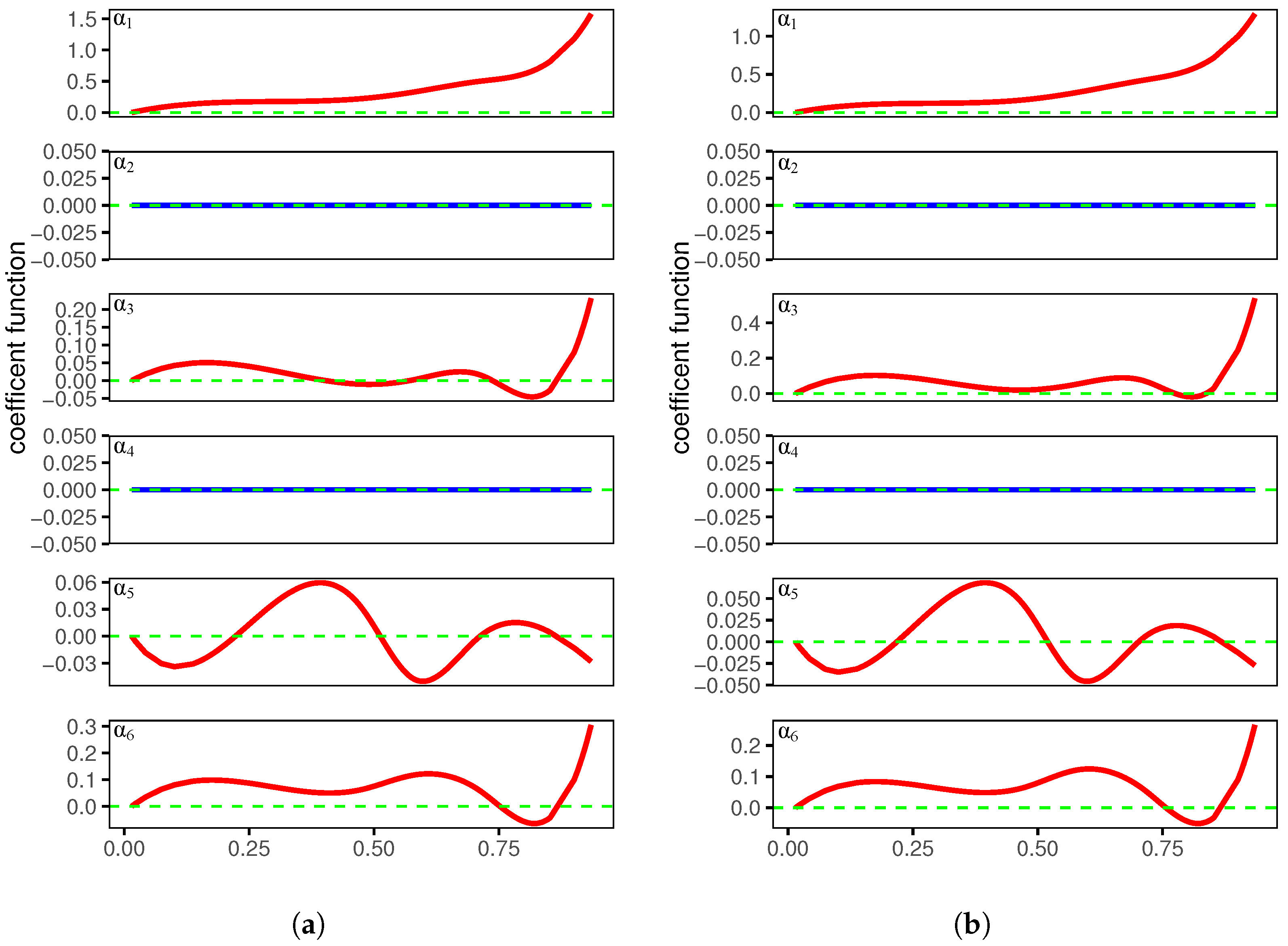
In previous studies, the affluence factor always had significantly positive effects on carbon dioxide emissions, and the effects were always set as a constant, see [37,38]. This phenomenon can be described by the following mechanism: among the three major industries, the secondary industry exhibits the highest dependence on energy consumption, followed by the tertiary industry. However, these two industries are also the pillar industries that drive economic development, implying a significant reliance on economic growth on energy consumption. Currently, fossil fuels constitute the primary energy source in the world, and their consumption leads to a substantial release of carbon dioxide. As indicated by existing research analyses, economic development contributes significantly to carbon emissions. It is well known that coal consumption among fossil fuels generates the most carbon dioxide, suggesting that the energy structure may directly influence the impact of economic development on carbon emissions. However, considering the significant variations in energy structures across and within different provinces, cities, and over different years, it may be unreasonable to measure this impact using a constant. Therefore, we wish to capture the potential heterogeneity of this impact using the coal consumption proportion (CCP), which is why we set the CCP as $u_{it}$ and six variables describing affluence as $z_{it1},\dots ,z_{it6}$.

Table 4 reports the estimated coefficient parameters, and Figure 1 depicts the estimated coefficient functions. There is not much difference between the results for SCAD and ALASSO, so we focus on the SCAD results in the following analysis. The spatial coefficient $\widehat{\rho }$ is not shrunk to zero and is positive, which means that neighboring provinces exhibit a substantial spatial positive correlation. The constant coefficients ${\widehat{\beta }}_2,{\widehat{\beta }}_3,{\widehat{\beta }}_4$, and ${\widehat{\beta }}_6$ are positive, and the mean values are estimated when EI, RDF, FIR, and FV change by 1% and CE changes by 0.35%, 0.087%, 0.245%, and 0.1%, respectively. ${\widehat{\beta }}_7$ is the only negative constant coefficient, which implies that as the public transportation passenger volume increases, carbon emissions tend to decrease. Public transportation is a low-carbon mode of transportation. The more people choose to travel by public transportation, the fewer people use private cars, leading to a reduction in carbon emissions. This provides the evidence for the negative coefficient ${\widehat{\beta }}_7$. The remaining coefficients are estimated to be zero, which means that they are excluded through variable selection. In addition, most of the coefficient functions in Figure 1 show an upward trend, which means that as coal consumption proportion increases, the contribution of affluence factors to carbon emission increases. Meanwhile, two function coefficients are removed through variable selection. This is generally consistent with the previous analysis in this section.

Table 4. Penalized estimators for the parametric components.

Method	$\widehat{\mathit{\rho }}$	${\widehat{\mathit{\beta }}}_{\mathbf{1}}$	${\widehat{\mathit{\beta }}}_{\mathbf{2}}$	${\widehat{\mathit{\beta }}}_{\mathbf{3}}$	${\widehat{\mathit{\beta }}}_{\mathbf{4}}$	${\widehat{\mathit{\beta }}}_{\mathbf{5}}$	${\widehat{\mathit{\beta }}}_{\mathbf{6}}$	${\widehat{\mathit{\beta }}}_{\mathbf{7}}$	${\widehat{\mathit{\beta }}}_{\mathbf{8}}$	${\widehat{\mathit{\sigma }}}^{\mathbf{2}}$
SCAD	0.154	0	0.350	0.087	0.245	0	0.100	−0.014	0	0.005
ALASSO	0.167	0	0.355	0.120	0.193	0	0.113	−0.017	0	0.005

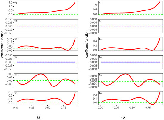
Figure 1. The estimated varying coefficient functions based on SCAD and ALASSO. (a) Varying coefficient derived from SCAD; (b) varying coefficient derived from ALASSO.

7. Discussion and Conclusions

Within the context of SVCSAR panel models with fixed effects, we developed a variable selection process that utilizes basis function approximations alongside the profile quasi-likelihood method. This approach allows for the simultaneous selection of significant variables in both parametric and nonparametric components, as well as the estimation of unknown coefficients. By selecting appropriate tuning parameters, we demonstrated that this selection process is consistent, and the estimators of constant coefficients exhibit the oracle property. Simulation results highlight the effectiveness of our proposed method in selecting variables and estimating both constant and varying coefficients. In this study, we assume that the dimensions of covariates X and Z remain fixed. Additionally, we also presented simulations in Section 5 and obtained desired results when the dimensions p and q were large. However, it is worth noting that our variable selection process may not be applicable to scenarios involving ultra-high-dimensional covariates. As a potential area for future research, exploring variable selection techniques for SVCSAR panel models with ultra-high-dimensional covariates would be of great interest.

References

- Anselin, L.; Hudak, S. Spatial econometrics in practice: A review of software options. Reg. Sci. Urban Econ. 1992, 22, 509–536. [Google Scholar] [CrossRef]
- Baltagi, B.H.; Heun Song, S.; Cheol Jung, B.; Koh, W. Testing for serial correlation, spatial autocorrelation and random effects using panel data. J. Econom. 2007, 140, 5–51. [Google Scholar] [CrossRef]
- Kapoor, M.; Kelejian, H.H.; Prucha, I.R. Panel data models with spatially correlated error components. J. Econom. 2007, 140, 97–130. [Google Scholar] [CrossRef]
- Baltagi, B.H.; Kao, C.; Liu, L. Asymptotic properties of estimators for the linear panel regression model with random individual effects and serially correlated errors: The case of stationary and non-stationary regressors and residuals. Econom. J. 2008, 11, 554–572. [Google Scholar] [CrossRef]
- Lee, L.F.; Yu, J. Estimation of spatial autoregressive panel data models with fixed effects. J. Econom. 2010, 154, 165–185. [Google Scholar] [CrossRef]
- Ai, C.; Zhang, Y. Estimation of partially specified spatial panel data models with fixed-effects. Econom. Rev. 2017, 36, 6–22. [Google Scholar] [CrossRef]
- Zhang, Y.; Sun, Y. Estimation of partially specified dynamic spatial panel data models with fixed-effects. Reg. Sci. Urban Econ. 2015, 51, 37–46. [Google Scholar] [CrossRef] [PubMed]
- Zhang, Y.; Shen, D. Estimation of semi-parametric varying-coefficient spatial panel data models with random-effects. J. Stat. Plan. Inference 2015, 159, 64–80. [Google Scholar] [CrossRef]
- Feng, S.; Tong, T.; Chiu, S.N. Statistical Inference for Partially Linear Varying Coefficient Spatial Autoregressive Panel Data Model. Mathematics 2023, 11, 4606. [Google Scholar] [CrossRef]
- Hu, X. Estimation in a semi-varying coefficient model for panel data with fixed effects. J. Syst. Sci. Complex. 2014, 27, 594–604. [Google Scholar] [CrossRef]
- He, B.; Hong, X.; Fan, G. Empirical likelihood for semi-varying coefficient models for panel data with fixed effects. J. Korean Stat. Soc. 2016, 45, 395–408. [Google Scholar] [CrossRef]
- Feng, S.; He, W.; Li, F. Model detection and estimation for varying coefficient panel data models with fixed effects. Comput. Stat. Data Anal. 2020, 152, 107054. [Google Scholar] [CrossRef]
- Feng, S.; Li, G.; Peng, H.; Tong, T. Varying coefficient panel data model with interactive fixed effects. Stat. Sin. 2021, 31, 935–957. [Google Scholar] [CrossRef]
- Sun, Y.; Carroll, R.; Li, D. Semiparametric estimation of fixed-effects panel data varying coefficient models. Adv. Econom. 2009, 25, 101–129. [Google Scholar]
- Tibshirani, R. Regression Shrinkage and Selection Via the Lasso. J. R. Stat. Soc. Ser. B (Methodol.) 1996, 58, 267–288. [Google Scholar] [CrossRef]
- Fan, J.; Li, R. Variable Selection via Nonconcave Penalized Likelihood and its Oracle Properties. J. Am. Stat. Assoc. 2001, 96, 1348–1360. [Google Scholar] [CrossRef]
- Zou, H. The Adaptive Lasso and Its Oracle Properties. J. Am. Stat. Assoc. 2006, 101, 1418–1429. [Google Scholar] [CrossRef]
- Wang, L.; Li, H.; Huang, J.Z. Variable Selection in Nonparametric Varying-Coefficient Models for Analysis of Repeated Measurements. J. Am. Stat. Assoc. 2008, 103, 1556–1569. [Google Scholar] [CrossRef]
- Li, R.; Liang, H. Variable selection in semiparametric regression modeling. Ann. Stat. 2008, 36, 261–286. [Google Scholar] [CrossRef]
- Wang, H.J.; Zhu, Z.; Zhou, J. Quantile regression in partially linear varying coefficient models. Ann. Stat. 2009, 37, 3841–3866. [Google Scholar] [CrossRef]
- Zhao, P.; Xue, L. Variable selection for semiparametric varying coefficient partially linear models. Stat. Probab. Lett. 2009, 79, 2148–2157. [Google Scholar] [CrossRef]
- Tian, R.; Xue, L.; Liu, C. Penalized quadratic inference functions for semiparametric varying coefficient partially linear models with longitudinal data. J. Multivar. Anal. 2014, 132, 94–110. [Google Scholar] [CrossRef]
- Tian, R.; Xue, L.; Hu, Y. Smooth-threshold GEE variable selection for varying coefficient partially linear models with longitudinal data. J. Korean Stat. Soc. 2015, 44, 419–431. [Google Scholar] [CrossRef]
- Li, R.; Mu, S.; Hao, R. Estimation and variable selection for partially linear additive models with measurement errors. Commun. Stat. Theory Methods 2021, 50, 1416–1445. [Google Scholar] [CrossRef]
- Ma, X.; Du, Y.; Wang, J. Model detection and variable selection for mode varying coefficient model. Stat. Methods Appl. 2022, 31, 321–341. [Google Scholar] [CrossRef]
- Liu, Y.; Wang, Z.; Tian, M.; Yu, K. Estimation and variable selection for generalized functional partially varying coefficient hybrid models. Stat. Pap. 2024, 65, 93–119. [Google Scholar] [CrossRef]
- Neyman, J.; Scott, E.L. Consistent Estimates Based on Partially Consistent Observations. Econometrica 1948, 16, 1–32. [Google Scholar] [CrossRef]
- Liu, X.; Chen, J.; Cheng, S. A penalized quasi-maximum likelihood method for variable selection in the spatial autoregressive model. Spat. Stat. 2018, 25, 86–104. [Google Scholar] [CrossRef]
- Xie, T.; Cao, R.; Du, J. Variable selection for spatial autoregressive models with a diverging number of parameters. Stat. Pap. 2020, 61, 1125–1145. [Google Scholar] [CrossRef]
- Luo, G.; Wu, M. Variable selection for semiparametric varying-coefficient spatial autoregressive models with a diverging number of parameters. Commun. Stat. Theory Methods 2021, 50, 2062–2079. [Google Scholar] [CrossRef]
- Lee, L.F. Asymptotic Distributions of Quasi-Maximum Likelihood Estimators for Spatial Autoregressive Models. Econometrica 2004, 72, 1899–1925. [Google Scholar] [CrossRef]
- Tian, R.; Xia, M.; Xu, D. Profile quasi-maximum likelihood estimation for semiparametric varying-coefficient spatial autoregressive panel models with fixed effects. Stat. Pap. 2024, 65, 5109–5143. [Google Scholar] [CrossRef]
- Kelejian, H.H.; Prucha, I.R. On the asymptotic distribution of the Moran I test statistic with applications. J. Econom. 2001, 104, 219–257. [Google Scholar] [CrossRef]
- He, X.; Fung, W.K.; Zhu, Z. Robust Estimation in Generalized Partial Linear Models for Clustered Data. J. Am. Stat. Assoc. 2005, 100, 1176–1184. [Google Scholar] [CrossRef]
- Stone, C.J. Optimal Global Rates of Convergence for Nonparametric Regression. Ann. Stat. 1982, 10, 1040–1053. [Google Scholar] [CrossRef]
- Dietz, T.; Rosa, E. Effects of population and affluence on CO2 emissions. Proc. Natl. Acad. Sci. USA 1997, 94, 175–179. [Google Scholar] [CrossRef]
- Wen, L.; Shao, H. Analysis of influencing factors of the carbon dioxide emissions in China’s commercial department based on the STIRPAT model and ridge regression. Environ. Sci. Pollut. Res. 2019, 26, 27138–27147. [Google Scholar] [CrossRef] [PubMed]
- Li, W.; Wang, W.; Wang, Y.; Qin, Y. Industrial structure, technological progress and CO2 emissions in China: Analysis based on the STIRPAT framework. Nat. Hazards 2017, 88, 1545–1564. [Google Scholar] [CrossRef]
Disclaimer/Publisher’s Note: The statements, opinions and data contained in all publications are solely those of the individual author(s) and contributor(s) and not of MDPI and/or the editor(s). MDPI and/or the editor(s) disclaim responsibility for any injury to people or property resulting from any ideas, methods, instructions or products referred to in the content. |
© 2025 by the authors. Licensee MDPI, Basel, Switzerland. This article is an open access article distributed under the terms and conditions of the Creative Commons Attribution (CC BY) license (https://creativecommons.org/licenses/by/4.0/).