Bifurcation Analysis in a Cross-Protection Model

Abstract

We analyze the population dynamics of a microbial cross-protection model and derive the exact conditions under which a Fold–Hopf bifurcation emerges. By applying center-manifold reduction and normal-form theory, we reduce the infinite-dimensional delay differential system to a finite-dimensional ordinary differential system, enabling rigorous bifurcation analysis. Numerical simulations reveal a rich repertoire of dynamical behaviors, including stable equilibria, sustained oscillations, and noise-induced irregularities. Our findings identify time-delay-induced Fold–Hopf bifurcation as a fundamental mechanism driving oscillatory coexistence in cross-protection mutualisms, for previously reported experimental observations.

1. Introduction

Microbial communities exist in a wide variety of environments [1,2,3] and play an important role in our world [4,5,6]. There is a competitive or cooperative relationship between microorganisms [7,8,9]. Understanding microbial interactions is ecologically important. In the presence of two antibiotics (ampicillin and chloramphenicol), two microorganisms may exhibit the phenomenon of cross-protection [10,11,12,13,14]. The cooperative nature of antibiotic inactivation allows a bacterial community of resistant strains to survive in a harsh environment, even if some strains are not individually resistant to each drug. Two Escherichia coli strains can form an effective cross-protection mutualism that protects each other under the presence of two antibiotics (ampicillin and chloramphenicol), which has been studied in [15]. Microbial communities are able to survive antibiotic exposures that would be lethal to individual cells under collective resistance. Vega and Jeff focus on how a community of bacteria can survive antimicrobial therapy whereas a single bacterium cannot [13]. It is important both clinically and ecologically to understand how bacterial populations survive antibiotic exposures.

These pioneering experimental studies [13,15] have unequivocally established cross-protection mutualism and its oscillatory dynamics as a robust biological phenomenon. However, while these works conclusively answered the question of ‘what’ exists, the underlying mathematical machinery—the ‘how’ and ‘why’ governed by nonlinear dynamics—has remained unclear. This gap motivates the present theoretical study. Our primary contribution is to identify, for the first time, the Fold–Hopf bifurcation induced by time delay as the fundamental intrinsic mechanism that generates the observed oscillatory coexistence. By developing a delay differential equation model, we move beyond descriptive recapitulation of the phenomenon to provide a quantitative, predictive framework. This framework is capable of calculating the critical conditions for oscillation emergence and systematically deciphering the decisive roles of delay in shaping population fate.

To theoretically unravel the mechanisms behind such microbial oscillations, an in-depth analysis of population dynamics is essential. The population density of many species fluctuates periodically over time, a phenomenon that cannot be fully explained by external factors such as seasonal changes [16]. These intrinsic cycles highlight the central role of nonlinear dynamics in ecology [17]. For instance, using a global population dynamics database, Kendall et al. [18] analyzed nearly 700 long-term animal time series and found that nearly 30% were cyclic. Similarly, Lindström et al. [19] documented periodic fluctuations in three species of tetraonids in Finland. Such studies underscore that complex dynamics, from stable equilibria to cycles and chaos, are inherent properties of nonlinear ecological models [20,21,22].

By developing a delay-differential model, we identify, for the first time, a time-delay-induced Fold–Hopf bifurcation as the intrinsic mechanism governing the transition from stable coexistence to robust oscillatory dynamics in microbial cross-protection. This bifurcation is not incidental: it yields a quantitative predictive criterion—the critical delay ${\tau }_0$—that precisely determines when stability yields to sustained oscillations. In doing so, our work moves beyond phenomenological description, establishing a mechanistic foundation for predicting and potentially controlling the fate of cooperative microbial populations under antibiotic stress.

The remainder of this paper is structured as follows: Section 2 details the theoretical analysis, reducing the infinite-dimensional delay differential equation to a finite-dimensional system via center manifold reduction and deriving the normal form for the Fold–Hopf bifurcation. Section 3 presents comprehensive numerical simulations that validate our theoretical findings and uncover the rich dynamics, including the role of time delay and noise. Building upon these results, Section 4 provides a discussion of the broader implications of our work and outlines promising future research directions. We conclude the paper with a summary of our main contributions in Section 5.

2. Reduction in Center Manifold and Calculation of Normal Forms

To investigate the dynamics of microbial cross-protection, we formulate a mathematical model that captures the temporal evolution of population densities and antibiotic concentrations over time, as follows:

$$\begin{array}{cc}\hfill {\displaystyle \frac{d{x}_1}{dt}}& ={\gamma }_1\left[x_4(t-{\tau }_4)\right]x_1(1-{\displaystyle \frac{x_1+x_2}{K}}),\hfill \\ \hfill {\displaystyle \frac{d{x}_2}{dt}}& ={\gamma }_2\left[x_3(t-{\tau }_3)\right]x_2(1-{\displaystyle \frac{x_1+x_2}{K}}),\hfill \\ \hfill {\displaystyle \frac{d{x}_3}{dt}}& =-{\displaystyle \frac{V_{max}{x}_3}{K_m+x_3}}{x}_1(t=0),\hfill \\ \hfill {\displaystyle \frac{d{x}_4}{dt}}& =-c_2{x}_4(t-{\tau }_4)x_2,\hfill \end{array}$$

(1)

where $x_1$ and $x_2$ denote the ampicillin- and chloramphenicol-resistant populations, respectively, while $x_3$ and $x_4$ represent the concentrations of ampicillin and chloramphenicol antibiotics. ${\gamma }_1\left[x_4(t-{\tau }_4)\right]$ and ${\gamma }_2\left[x_3(t-{\tau }_3)\right]$ represent antibiotic concentration-dependent growth rates. We assume ${\gamma }_1\left[x_4(t-{\tau }_4)\right]={\displaystyle \frac{{\gamma }_1^R}{1+x_4(t-{\tau }_4)/IC{50}_{12}}}$ and ${\gamma }_2\left[x_3(t-{\tau }_3)\right]=-{\gamma }_2^D+{\displaystyle \frac{{\gamma }_2^R+{\gamma }_2^D}{1+x_3(t-{\tau }_3)/IC{50}_{21}}}$. K is the carrying capacity. ${\gamma }_1^R$ is the growth rate of ampicillin-resistant cells in the absence of chloramphenicol. ${\gamma }_2^R$ is the growth rate of chloramphenicol-resistant cells in the absence of ampicillin. ${\gamma }_2^D$ is the death rate of chloramphenicol-resistant cells ampicillin at high concentrations. $IC{50}_{12}$ refers to the inhibitory concentration of ampicillin that affects chloramphenicol-resistant cells, while $IC{50}_{21}$ represents the inhibitory concentration of ampicillin-resistant cells in chloramphenicol. $K_m$ is the Michaelis–Menten constant for ampicillin inactivation. $c_2$ is the chloramphenicol inactivation rate.

The mathematical formulation in (1) provides a mechanistic representation of the cross-protection mutualism experimentally characterized in [15]. Each component captures essential biological processes: the growth rates ${\gamma }_1\left[x_4(t-{\tau }_4)\right]$ and ${\gamma }_2\left[x_3(t-{\tau }_3)\right]$ encode the antibiotic-dependent growth inhibition and mutual protection dynamics, with time delays ${\tau }_3$ and ${\tau }_4$ representing the finite duration for enzyme production and antibiotic inactivation. The functional forms reflect documented biological responses—the Hill-type inhibition captures concentration-dependent suppression, while the carrying capacity K constrains population densities to experimentally observed ranges. This formulation bridges molecular resistance mechanisms with population-level dynamics through physiologically grounded mathematical representations.

The system (1) is a system of delay differential equations (DDEs). A fundamental distinction between DDEs and ordinary differential equations is that the evolution of a DDE depends not only on its present state but also on its history. Consequently, to determine a unique solution for $t>0$, the initial condition required is not a finite-dimensional vector $(x_1\left(0\right),x_2\left(0\right),x_3\left(0\right),x_4\left(0\right))\in {\mathbb{R}}^4$, but rather an initial function defined on the entire delay interval $[-{\tau }_{max},0]$, where ${\tau }_{max}=max\{{\tau }_3,{\tau }_4\}$. Formally, the initial condition is $\varphi \left(\theta \right)=({\varphi }_1\left(\theta \right),{\varphi }_2\left(\theta \right),{\varphi }_3\left(\theta \right),{\varphi }_4\left(\theta \right))$ for $\theta \in [-{\tau }_{max},0]$. The phase space of the system is therefore the Banach space $\mathcal{C}([-{\tau }_{max},0],{\mathbb{R}}^4)$ of continuous functions mapping the delay interval into ${\mathbb{R}}^4$. Since specifying a continuous function requires an infinite amount of information, this phase space is infinite-dimensional [23].

The system admits a boundary equilibrium at $(x_1^{*},x_2^{*},0,0)$, where $x_1^{*}$ and $x_2^{*}$ satisfy the carrying capacity constraint:

$$1-{\displaystyle \frac{x_1^{*}+x_2^{*}}{K}}=0.$$

where the system is linearized in the vicinity of the equilibrium point. Defining the deviation variables as $u_1=x_1-x_1^{*}$, $u_2=x_2-x_2^{*}$, $u_3=x_3$, and $u_4=x_4$, the linearized system is obtained as

$$\begin{array}{cc}\hfill {\displaystyle \frac{d{u}_1}{dt}}& =-a{x}_1^{*}{u}_1\left(t\right)-a{x}_1^{*}{u}_2\left(t\right),\hfill \\ \hfill {\displaystyle \frac{d{u}_2}{dt}}& =-b{x}_2^{*}{u}_1\left(t\right)-b{x}_2^{*}{u}_2\left(t\right),\hfill \\ \hfill {\displaystyle \frac{d{u}_3}{dt}}& =-c{u}_3\left(t\right),\hfill \\ \hfill {\displaystyle \frac{d{u}_4}{dt}}& =-d{u}_4(t-{\tau }_4).\hfill \end{array}$$

Local stability is assessed via linearization around the equilibrium, yielding a transcendental characteristic equation whose eigenvalue structure determines the stability properties of the system. To derive the characteristic equation, we assume solutions of the form $u\left(t\right)=e^{\lambda t}v$, where $\lambda$ is the characteristic exponent and v is the corresponding eigenvector. Substituting this exponential form into the linearized system, we analyze each component separately.

From the equations for $u_1$ and $u_2$, we obtain

$$\left[\begin{array}{cc}\lambda +a{x}_1^{*}& a{x}_1^{*}\\ b{x}_2^{*}& \lambda +b{x}_2^{*}\end{array}\right]\left[\begin{array}{c}{u}_1\\ u_2\end{array}\right]=0,$$

and the characteristic equation for this subsystem is given by the determinant

$$det\left[\begin{array}{cc}\lambda +a{x}_1^{*}& a{x}_1^{*}\\ b{x}_2^{*}& \lambda +b{x}_2^{*}\end{array}\right]=0,$$

which expands to

$$(\lambda +a{x}_1^{*})(\lambda +b{x}_2^{*})-ab{x}_1^{*}{x}_2^{*}=0.$$

From the equation for $u_3$, we obtain

$$\lambda +c=0.$$

From the equation for $u_4$, we obtain

$$\lambda +d{e}^{-\lambda \tau }=0.$$

Since the system is decoupled, the overall characteristic equation is the product of the characteristic equations from each subsystem:

$$(\lambda +c)(\lambda +d{e}^{-\lambda \tau })[(\lambda +a{x}_1^{*})(\lambda +b{x}_2^{*})-ab{x}_1^{*}{x}_2^{*}]=0,$$

(2)

and the third factor requires explicit expansion:

$$\begin{array}{cc}& (\lambda +a{x}_1^{*})(\lambda +b{x}_2^{*})-ab{x}_1^{*}{x}_2^{*}\hfill \\ & ={\lambda }^2+\lambda (a{x}_1^{*}+b{x}_2^{*})+ab{x}_1^{*}{x}_2^{*}-ab{x}_1^{*}{x}_2^{*}\hfill \\ & ={\lambda }^2+\lambda (a{x}_1^{*}+b{x}_2^{*}),\hfill \end{array}$$

Thus, the simplified characteristic equation becomes

$$(\lambda +c)(\lambda +d{e}^{-\lambda \tau })\lambda (\lambda +a{x}_1^{*}+b{x}_2^{*})=0,$$

where $a={\displaystyle \frac{{\gamma }_1^R}{K}}$, $b={\displaystyle \frac{{\gamma }_2^R}{K}}$, $c={\displaystyle \frac{V_{max}}{K_m}}{x}_{10}$, $x_{10}=x_1(t=0)$, and $d=c_2{x}_2^{*}$. It is seen that $\lambda =0$ is one root of the model (1). The roots of the characteristic equation are

$$\begin{array}{cc}& \lambda =0(\mathrm{from}\lambda =0),\hfill \\ & \lambda =-(a{x}_1^{*}+b{x}_2^{*}),\hfill \\ & \lambda =-c,\hfill \\ & \mathrm{and}\mathrm{roots}\mathrm{from}\lambda +d{e}^{-\lambda \tau }=0.\hfill \end{array}$$

For Hopf bifurcation analysis, we focus on the transcendental equation

$$\lambda +d{e}^{-\lambda \tau }=0,$$

A Hopf bifurcation occurs when a pair of complex conjugate eigenvalues crosses the imaginary axis, leading to the emergence of sustained oscillations from a previously stable equilibrium. This transition is characterized by the existence of purely imaginary eigenvalues $\lambda =\pm i\omega$ ($\omega >0$) at the critical parameter value.

To identify such a bifurcation in our system, we substitute $\lambda =i\omega$ ($\omega >0$) into the characteristic equation, yielding separate real and imaginary parts:

$$\left\{\begin{array}{c}dcos\left(\omega \tau \right)=0,\hfill \\ dsin\left(\omega \tau \right)=\omega .\hfill \end{array}\right.$$

Solving for $\tau$,

$${\tau }_k={\displaystyle \frac{(2k+1)\pi }{2\omega }},$$

and substituting into the second equation and using $sin({\displaystyle \frac{\pi }{2}}+k\pi )={(-1)}^k$,

$$\omega =d{(-1)}^k,$$

For positive frequency $\omega >0$ and even k, we obtain the critical parameters:

$${\omega }_0=d,{\tau }_k={\displaystyle \frac{(2k+1)\pi }{2d}}.$$

At these critical parameter values, the characteristic equation possesses a pair of purely imaginary eigenvalues $\lambda =\pm i{\omega }_0$. We confirm the occurrence of a non-degenerate Hopf bifurcation by verifying the transversality condition, ensuring that the eigenvalues cross the imaginary axis with non-zero speed. Differentiating the characteristic equation with respect to $\tau$,

$${\displaystyle \frac{d\lambda }{d\tau }}-d{e}^{-\lambda \tau }\left(-\lambda -\tau {\displaystyle \frac{d\lambda }{d\tau }}\right)=0,$$

and solving for the derivative,

$${\displaystyle \frac{d\lambda }{d\tau }}={\displaystyle \frac{\lambda d{e}^{-\lambda \tau }}{1-\tau d{e}^{-\lambda \tau }}},$$

At the critical point $\lambda =i{\omega }_0$ with ${\omega }_0=d$ and $e^{-i{\omega }_0{\tau }_k}=-i$,

$${\left.{\displaystyle \frac{d\lambda }{d\tau }}\right|}_{\lambda =i{\omega }_0}={\displaystyle \frac{i{d}^2}{1+id{\tau }_k}},$$

and computing the reciprocal and extracting the real part,

$$\Re e{\left({\displaystyle \frac{d\lambda }{d\tau }}\right)}^{-1}={\displaystyle \frac{1}{d^2}}\ne 0.$$

This non-zero value confirms that eigenvalues cross the imaginary axis with non-zero speed, satisfying the transversality condition for a genuine Hopf bifurcation.

Subsequently, building upon the established framework for reducing the infinite-dimensional delay differential model (1) to a finite-dimensional ordinary differential system using center manifold theory [23] and the normal form method [24], we now present the detailed mathematical derivation.

If we introduce small perturbations and rescale time as $t\mapsto t/({\tau }_0+{\mu }_2)$, we recast model (1) in a form amenable to the center manifold reduction and normal form analysis.

$$\begin{array}{cc}\hfill {\displaystyle \frac{d{x}_1}{dt}}& =(-{\displaystyle \frac{x_1^{*}{\gamma }_1^R-{\mu }_1}{K}})x_1-{\displaystyle \frac{x_1^{*}{\gamma }_1^R}{K}}{x}_2-{\displaystyle \frac{{\gamma }_1^R}{K}}{x}_1^2-{\displaystyle \frac{{\gamma }_1^R}{K}}{x}_1{x}_2,\hfill \\ \hfill {\displaystyle \frac{d{x}_2}{dt}}& =(-{\displaystyle \frac{x_2^{*}{\gamma }_2^R}{K}})x_1-{\displaystyle \frac{x_2^{*}{\gamma }_2^R}{K}}{x}_2-{\displaystyle \frac{{\gamma }_2^R}{K}}{x}_2^2-{\displaystyle \frac{{\gamma }_2^R}{K}}{x}_1{x}_2,\hfill \\ \hfill {\displaystyle \frac{d{x}_3}{dt}}& =-{\displaystyle \frac{V_{max}{x}_{10}}{K_m}}{x}_3+{\displaystyle \frac{V_{max}{x}_{10}}{K_m^2}}{x}_3^2,\hfill \\ \hfill {\displaystyle \frac{d{x}_4}{dt}}& =-c_2{x}_2^{*}{x}_4(t-{\tau }_4)-c_2{x}_2{x}_4(t-{\tau }_4),\hfill \end{array}$$

(3)

where ${\mu }_1$ and ${\mu }_2$ are perturbations.

The linearization of the system (3) around the origin is given by

$$\begin{array}{ccc}\hfill \dot{U}& =& A_{1}U+A_{2}U(t-1),\hfill \end{array}$$

(4)

where

$$A_1=({\tau }_0+{\mu }_2)\left(\begin{array}{cccc}-a{x}_1^{*}-{\mu }_1& -a{x}_1^{*}& 0& 0\\ -b{x}_2^{*}& -b{x}_2^{*}& 0& 0\\ 0& 0& -c& 0\\ 0& 0& 0& 0\end{array}\right), A_2=({\tau }_0+{\mu }_2)\left(\begin{array}{cccc}0& 0& 0& 0\\ 0& 0& 0& 0\\ 0& 0& 0& 0\\ 0& 0& 0& -d\end{array}\right).$$

The system (3) can be rewritten as an abstract differential equation

$$\begin{array}{ccc}\hfill \dot{U}\left(t\right)& =& L\left(\mu \right)U_t+F(U_t,\mu ),\hfill \end{array}$$

(5)

where $U_t=U_t\left(\theta \right)=U(t+\theta )$, $-1\le \theta \le 0$. $L\left(\mu \right)$ is a one-parameter family of bounded linear operators in $\mathcal{C}=\mathcal{C}([-1,0],R^4)$ defined by

$$\begin{array}{ccc}\hfill L\left(\mu \right)\varphi & =& A_1\varphi \left(0\right)+A_2\varphi (-1).\hfill \end{array}$$

(6)

By the Riese representation theorem, there exists a bounded variation function $\eta (\theta ,\mu )$ in $[-1,0]\to R^4$ such that

$$\begin{array}{ccc}\hfill L\left(\mu \right)\phi & =& {\int }_{-1}^{0}d\eta (\theta ,\mu )\phi \left(\theta \right).\hfill \end{array}$$

For $\phi \in \mathcal{C}$, we have

$$\begin{array}{ccc}\hfill F(\phi ,\mu )& =& ({\tau }_0+{\mu }_2)\left(\begin{array}{c}-a{\phi }_1^2\left(0\right)-a{\phi }_1\left(0\right){\phi }_2\left(0\right)+ag{\phi }_1\left(0\right){\phi }_4(-1)\\ -b{\phi }_2^2\left(0\right)-b{\phi }_1\left(0\right){\phi }_2\left(0\right)\\ mc{\phi }_3^2\left(0\right)\\ -c_2{\phi }_2\left(0\right){\phi }_4(-1)\end{array}\right).\hfill \end{array}$$

where $g={\displaystyle \frac{1}{IC{50}_{12}}}$ and $m={\displaystyle \frac{1}{k_m}}$.

To construct the center manifold and derive the normal form, we first compute the eigenvectors corresponding to the critical eigenvalues of the linearized system. At the critical point $\mu =0$, the linear operator $L\left(0\right)$ defined in Equation (6) has a zero eigenvalue and a pair of purely imaginary eigenvalues $\pm i{\omega }_0{\tau }_0$. We now derive the corresponding right and left eigenvectors and normalize them using the bilinear form.

To determine the right eigenvectors of $L\left(0\right)$, let $\Phi \left(\theta \right)=({\varphi }_1\left(\theta \right),{\varphi }_2\left(\theta \right),{\varphi }_3\left(\theta \right),{\varphi }_4\left(\theta \right))$ for $\theta \in [-1,0]$ denote the right eigenfunctions corresponding to the eigenvalues $\lambda =0,\pm i{\omega }_0{\tau }_0$. We solve

$$L\left(0\right)\Phi =\lambda \Phi .$$

For $\lambda =0$,

$$A_1\Phi \left(0\right)+A_2\Phi (-1)=0,$$

which yields the eigenvector

$${\varphi }_0\left(\theta \right)=\left(\begin{array}{c}1\\ -1\\ 0\\ 0\end{array}\right).$$

For $\lambda =i{\omega }_0{\tau }_0$,

$$A_1\varphi \left(0\right)+A_2\varphi (-1)=i{\omega }_0{\tau }_0\varphi \left(0\right),$$

which gives the eigenvector

$${\varphi }_1\left(\theta \right)=\left(\begin{array}{c}1\\ q_1\\ q_2\\ q_3\end{array}\right)e^{i{\omega }_0{\tau }_0\theta },$$

where

$$q_1=1+{\displaystyle \frac{i{\omega }_0}{a{x}_1^{*}}},q_2=q_3=0.$$

The complex conjugate ${\varphi }_2\left(\theta \right)=\overline{{\varphi }_1\left(\theta \right)}$ corresponds to $\lambda =-i{\omega }_0{\tau }_0$.

To solve for the left eigenvectors of the adjoint operator $L^{*}\left(0\right)$, we define it on the dual space $C^{*}=C([0,1],{\mathbb{R}}^{4*})$ as follows:

$$L^{*}\left(0\right)\psi \left(s\right)=-A_1^T\psi \left(0\right)-A_2^T\psi \left(1\right),s\in [0,1].$$

We seek left eigenfunctions $\Psi \left(s\right)$ satisfying

$$L^{*}\left(0\right)\Psi =\lambda \Psi .$$

For $\lambda =0$,

$$-A_1^T\psi \left(0\right)-A_2^T\psi \left(1\right)=0,$$

yielding

$${\psi }_0\left(s\right)=\left(\begin{array}{c}{\displaystyle \frac{1}{2}}\\ -{\displaystyle \frac{1}{2}}\\ 0\\ 0\end{array}\right).$$

For $\lambda =-i{\omega }_0{\tau }_0$,

$$-A_1^T\psi \left(0\right)-A_2^T\psi \left(1\right)=-i{\omega }_0{\tau }_0\psi \left(s\right),$$

we obtain

$${\psi }_1\left(s\right)=\rho \left(\begin{array}{c}1\\ q_1^{*}\\ q_2^{*}\\ q_3^{*}\end{array}\right)e^{-i{\omega }_0{\tau }_{0}s},$$

where

$$q_1^{*}={\displaystyle \frac{i{\omega }_0}{a{x}_1^{*}}}-1,q_2^{*}=q_3^{*}=0,\rho ={\displaystyle \frac{1}{q_1{q}_1^{*}}}.$$

The conjugate ${\psi }_2\left(s\right)=\overline{{\psi }_1\left(s\right)}$ corresponds to $\lambda =i{\omega }_0{\tau }_0$.

To normalize the eigenfunctions, we employ the bilinear form

$$⟨\psi ,\varphi ⟩=\psi \left(0\right)\varphi \left(0\right)-{\int }_{-1}^0{\int }_{\xi }^0\psi (\xi -\theta )d\eta \left(\theta \right)\varphi \left(\xi \right)d\xi ,\eta \left(\theta \right)≔,\eta (\theta ,0),$$

which is constructed via the formal adjoint theory for functional differential equations (FDEs) so as to decompose the phase space. Here, $\psi \in C^{*}=C([0,1],{\mathbb{R}}^{4*})$ and $\varphi \in C$; $P\subset C$ denotes the eigenspace associated with eigenvalues of zero real part, while $P^{*}\subset C^{*}$ is the corresponding center space for the adjoint equation. Imposing the orthonormality conditions

$$⟨{\psi }_0,{\varphi }_0⟩=1,⟨{\psi }_1,{\varphi }_1⟩=1,⟨{\psi }_0,{\varphi }_1⟩=⟨{\psi }_1,{\varphi }_0⟩=0$$

ensures that the infinite-dimensional flow is projected onto the center manifold in a well-defined manner, thereby yielding the correct finite-dimensional reduced system required for the subsequent normal-form computation.

Thus, the phase space C can be decomposed by eigenvalues 0 and $\pm i{\tau }_0{\omega }_0$ as $\mathcal{C}=P⨁Q$, where $Q=\phi \in \mathcal{C}:<\psi ,\phi >=0$ for all $\psi \in P^{*}$. The bases are denoted by $\Phi \left(\theta \right)$ and $\Psi \left(s\right)$ in P, $P^{*}$ as follows:

$$\begin{array}{ccc}& & \Phi \left(\theta \right)=\left(\begin{array}{ccc}1& e^{i{\omega }_0{\tau }_0\theta }& e^{-i{\omega }_0{\tau }_0\theta }\\ -1& q_1{e}^{i{\omega }_0{\tau }_0\theta }& {\overline{q}}_1{e}^{-i{\omega }_0{\tau }_0\theta }\\ 0& q_2{e}^{i{\omega }_0{\tau }_0\theta }& {\overline{q}}_2{e}^{-i{\omega }_0{\tau }_0\theta }\\ 0& q_3{e}^{i{\omega }_0{\tau }_0\theta }& {\overline{q}}_3{e}^{-i{\omega }_0{\tau }_0\theta }\end{array}\right),-1\le \theta \le 0\hfill \\ & & \Psi \left(s\right)=\left(\begin{array}{cccc}{\displaystyle \frac{1}{2}}& -{\displaystyle \frac{1}{2}}& 0& 0\\ \rho e^{-i{\omega }_0{\tau }_{0}s}& \rho q_1^{*}{e}^{-i{\omega }_0{\tau }_{0}s}& \rho q_2^{*}{e}^{-i{\omega }_0{\tau }_{0}s}& \rho q_3^{*}{e}^{-i{\omega }_0{\tau }_{0}s}\\ \overline{\rho }{e}^{i{\omega }_0{\tau }_{0}s}& \overline{\rho }{\overline{q}}_1^{*}{e}^{i{\omega }_0{\tau }_{0}s}& \overline{\rho }{\overline{q}}_2^{*}{e}^{i{\omega }_0{\tau }_{0}s}& \overline{\rho }{\overline{q}}_3^{*}{e}^{i{\omega }_0{\tau }_{0}s}\end{array}\right),0\le s\le 1\hfill \end{array}$$

where $q_1=1+{\displaystyle \frac{i{\omega }_0}{a{x}_1^{*}}}$, $q_2=q_3=0$, $q_1^{*}={\displaystyle \frac{i{\omega }_0}{a{x}_1^{*}}}-1$, $q_2^{*}=q_3^{*}=0$, and $\rho ={\displaystyle \frac{1}{q_1{q}_1^{*}}}$.

The constructed eigenbasis $\Phi \left(\theta \right)$ and $\Psi \left(s\right)$ provides profound insight into the dynamical structure of the cross-protection system near the Fold–Hopf bifurcation:

The zero eigenvalue mode ($\lambda =0$) corresponds to neutral stability along the direction of total population conservation, reflecting the trade-off between the two bacterial strains in utilizing the shared carrying capacity.

The imaginary eigenvalue modes ($\lambda =\pm i{\omega }_0{\tau }_0$) capture the oscillatory dynamics arising from the delayed feedback between antibiotic inactivation and population growth. The phase relationships encoded in $q_1$ and $q_1^{*}$ quantify the temporal coordination between strain interactions.

The left eigenvectors $\Psi \left(s\right)$ represent the adjoint modes that determine how perturbations in antibiotic concentrations and population densities couple into the critical directions, essentially defining the system’s susceptibility to external disturbances.

The parameter $\rho =1/\left(q_1{q}_1^{*}\right)$ serves as a coupling coefficient that normalizes the interaction strength between the oscillatory modes, ensuring that the reduced dynamics on the center manifold accurately preserve the essential nonlinear interactions of the original infinite-dimensional system.

We project the infinite dimensional flow on $\mathcal{C}$ onto the finite dimensional manifold P [24]. We consider the enlarged phase space $BC$ of the function from $[-1,0]$ to $R^4$, which is continuous at $[-1,0]$. In the space $BC$, the abstract differential Equation (5) can be written as an abstract form

$$\begin{array}{ccc}\hfill {\displaystyle \frac{d{U}_t}{dt}}& =& A{U}_t+X_{0}G(U_t,\mu ),\hfill \end{array}$$

(7)

where $X_0$ is the $4\times 4$ matrix-valued function defined by $X_0\left(\theta \right)=0$ for $\theta \in [-1,0)$ and $X_0\left(0\right)=I$,

$$\begin{array}{ccc}& & G(\phi ,\mu )=\left(L\right(\mu )-L(0\left)\right)\phi +F(\phi ,\mu )\hfill \\ & & =\left(\begin{array}{c}-a{x}_1^{*}{\mu }_2({\phi }_1\left(0\right)+{\phi }_2\left(0\right))-({\tau }_0+{\mu }_2){\mu }_1{\phi }_1\left(0\right)\\ -b{x}_2^{*}{\mu }_2({\phi }_1\left(0\right)+{\phi }_2\left(0\right))\\ -c{\mu }_2{\phi }_3\left(0\right)\\ -d{\mu }_2{\phi }_4(-1)\end{array}\right)\hfill \\ & & +\left(\begin{array}{c}-({\tau }_0+{\mu }_2)(a{\phi }_1^2\left(0\right)+a{\phi }_1\left(0\right){\phi }_2\left(0\right)-ag{\phi }_1\left(0\right){\phi }_4(-1))\\ -({\tau }_0+{\mu }_2)(b{\phi }_2^2\left(0\right)+b{\phi }_1\left(0\right){\phi }_2\left(0\right))\\ ({\tau }_0+{\mu }_2)mc{\phi }_3^2\left(0\right)\\ -({\tau }_0+{\mu }_2)c_2{\phi }_2\left(0\right){\phi }_4(-1)\end{array}\right).\hfill \end{array}$$

A is defined by $A\phi =\dot{\phi }+X_0[L\left(0\right)\phi -\dot{\phi }\left(0\right)]$. The continuous projection is defined as $\pi :BC\to P,\pi (\phi +X_{0c})=\Phi [(\Psi ,\phi )+\Psi {\left(0\right)}_c]$. The enlarged phase space can be decomposed by 0 and $\pm i{\omega }_0$ as $BC=P⨁Ker\pi$. We use the composition

$$\begin{array}{ccc}\hfill U_t& =& \Phi \left(\theta \right)z+y=\left(\begin{array}{c}{z}_1+z_2{e}^{i{\omega }_0{\tau }_0\theta }+z_3{e}^{-i{\omega }_0{\tau }_0\theta }+y_1\left(\theta \right)\\ -z_1+q_1{z}_2{e}^{i{\omega }_0{\tau }_0\theta }+{\overline{q}}_1{z}_3{e}^{-i{\omega }_0{\tau }_0\theta }+y_2\left(\theta \right)\\ z_1+y_3\left(\theta \right)\\ -z_1+y_4\left(\theta \right)\end{array}\right),\hfill \end{array}$$

Thus, (7) can be written as the following:

$$\begin{array}{ccc}\hfill \dot{z}& =& Bz+\Psi \left(0\right)G(\Phi z+y,\mu )\hfill \\ \hfill \dot{y}& =& A_{Q^1}y+(I-\pi )X_{0}G(\Phi z+y,\mu )\hfill \end{array}$$

For $z\in R^3$, $y\in Q^1=Q\bigcap C^1\subset Ker\pi$, where $A_{Q^1}$ is the restriction of A as an operator from $Q^1$ to the Banach space $Ker\pi$. Let $M^2$ denote the operator defined in $V_2^7(R^3\times Ker\pi )$ with values in the same space by $M_2(p,h)=(M_2^{1}p,M_2^{2}h)$ and $\left(M_2^{1}p\right)(z,\mu )=D_{z}p(z,\mu )Bz-Bp(z,\mu )$. We choose the decomposition $V_2^7\left(R^3\right)=I_m\left(M_2^1\right)⨁I_m{\left(M_2^1\right)}^c$ with complementary space $I_m{\left(M_2^1\right)}^c$ spanned by the elements

$$\left(\begin{array}{c}{z}_1^2\\ 0\\ 0\end{array}\right);\left(\begin{array}{c}{z}_2{z}_3\\ 0\\ 0\end{array}\right);\left(\begin{array}{c}{z}_1{\mu }_i\\ 0\\ 0\end{array}\right);\left(\begin{array}{c}{\mu }_1^2\\ 0\\ 0\end{array}\right);\left(\begin{array}{c}{\mu }_2^2\\ 0\\ 0\end{array}\right);$$

$$\left(\begin{array}{c}0\\ z_1{z}_2\\ 0\end{array}\right);\left(\begin{array}{c}0\\ z_2{\mu }_i\\ 0\end{array}\right);\left(\begin{array}{c}0\\ 0\\ z_1{z}_3\end{array}\right);\left(\begin{array}{c}0\\ 0\\ z_3{\mu }_i\end{array}\right).$$

For the complete mathematical derivation of the normal form coefficients, see Appendix A. According to [24], the normal form of (5) on the center manifold of the origin near $\mu =0$ can be written as

$$\begin{array}{cc}\hfill {\dot{z}}_1& =f_{a1}{\mu }_1{z}_1+f_{a2}{z}_1^2+f_{a3}{z}_2{z}_3+\cdots ,\hfill \\ \hfill {\dot{z}}_2& =i{\omega }_0{\tau }_0{z}_2+f_{b1}{\mu }_1{z}_2+f_{b2}{\mu }_2{z}_2+f_{b3}{z}_1{z}_2+\cdots ,\hfill \\ \hfill {\dot{z}}_3& =-i{\omega }_0{\tau }_0{z}_3+{\overline{f}}_{b1}{\mu }_1{z}_3+{\overline{f}}_{b2}{\mu }_2{z}_3+{\overline{f}}_{b3}{z}_1{z}_3+\cdots ,\hfill \end{array}$$

(8)

where $f_{a1}=-{\displaystyle \frac{1}{2}}{\tau }_0$, $f_{a2}=-{\displaystyle \frac{1}{2}}{\tau }_{0}ag$, $f_{a3}=-2a{\tau }_0+{\tau }_{0}b(1+q_1{\overline{q}}_1)$, $f_{b1}=-\rho {\tau }_0$, $f_{b2}=-\rho a{x}_1^{*}(1+q_1)-\rho q_1^{*}b{x}_2^{*}(1+q_1)$, and $f_{b3}=\rho {\tau }_0(1-2a-a{q}_1)+\rho q_1^{*}{\tau }_0(1+b{q}_1)$.

We change these variables $z_1={\omega }_1$, $z_2=rcos\theta -irsin\theta$, and $z_3=rcos\theta +irsin\theta$. Then, (8) becomes the planar system for $({\omega }_1,r)$ with $r\ge 0$:

$$\begin{array}{cc}\hfill & {\dot{\omega }}_1=f_{a1}{\mu }_1{\omega }_1+f_{a2}{\omega }_1^2+f_{a3}{r}^2+\cdots ,\hfill \\ \hfill & \dot{r}=(\Re f_{b1}{\mu }_1+\Re f_{b2}{\mu }_2+\Re f_{b3}{\omega }_1)r+\cdots ,\hfill \end{array}$$

(9)

where $\Re f_{bi}=\Re e{f}_{bi}$, $i=1,2,3.$

The equilibria of (9) are $E_1=(0,0)$ and $E_2=(-{\displaystyle \frac{f_{a1}}{f_{a2}}}{\mu }_1,0)$ with $r=0$, and $E_3=(-{\displaystyle \frac{\Re f_{b1}}{\Re f_{b3}}}{\mu }_1-{\displaystyle \frac{\Re f_{b2}}{\Re f_{b3}}}{\mu }_2,r_0)$ with $r>0$, where $r_0>0$ and $r_0^2=-{\displaystyle \frac{1}{f_{a3}\Re f_{b3}^2}}[(f_{a2}\Re f_{b1}^2-f_{a1}\Re f_{b1}{f}_{b3}){\mu }_1^2+\Re f_{b2}(2f_{a2}\Re f_{b1}-f_{a1}\Re f_{b3}){\mu }_1{\mu }_2+f_{a2}\Re f_{b2}^2{\mu }_2^2]$.

3. Numerical Simulations and Result Analysis

3.1. Basic Dynamics and Bifurcation Simulation

Our numerical simulations employ parameter values rigorously calibrated against the experimental cross-protection system of Yurtsev et al. [15]. Growth parameters (${\gamma }_1^R=7$, ${\gamma }_2^R=1.21$) reflect measured replication rates in LB medium, while inhibition constants ($IC{50}_{12}=1.3$, $IC{50}_{21}=1.65$) are derived from quantitative dose–response analyses of strain susceptibility. The carrying capacity $K=2.5$ corresponds to experimentally observed saturation densities, and the death rate ${\gamma }_2^D=0.25$ quantifies the bactericidal effect of ampicillin on chloramphenicol-resistant cells. Enzyme kinetic parameters ($V_{max}=20$, $K_m=12$, $c_2=10$) characterize antibiotic inactivation rates consistent with the catalytic efficiencies of $\beta$-lactamase and chloramphenicol acetyltransferase. The time delay parameters (${\tau }_3=0.8$, ${\tau }_4$ as control parameter) represent the finite duration required for enzyme production and extracellular antibiotic inactivation.

Our numerical analysis aims to demonstrate that the theoretically predicted Fold–Hopf bifurcation provides a mechanistic explanation for the oscillatory coexistence observed experimentally. The critical delay ${\tau }_0=0.48$, emerging from our bifurcation analysis in Section 2, serves as a quantitative benchmark. We systematically test this prediction by selecting ${\tau }_4=0.46$ and ${\tau }_4=0.5$ to bracket this theoretical threshold, thereby demonstrating the fundamental stability–oscillation transition that underlies the cross-protection mutualism.

As shown in Figure 1a,b, the equilibrium point $(1.41,1.07,0,0)$ of system (1) exhibits asymptotic stability when ${\tau }_4=0.46$. However, both the ampicillin-resistant and chloramphenicol-resistant populations display transient oscillatory behavior over a finite time interval before gradually decaying to the equilibrium state. These transient oscillations demonstrate the dynamic interplay between antibiotic inhibition and cross-protection mechanisms during the initial phase of population establishment.

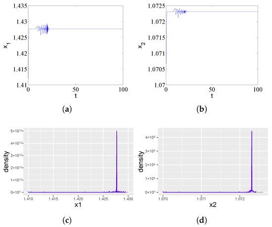
Figure 1. Asymptotic stability of the equilibrium point $(1.41,1.07,0,0)$ in system (1) for a subcritical time delay ${\tau }_4=0.46<{\tau }_0=0.48$. (a) Time series of the ampicillin-resistant population ($x_1$) showing damped oscillations converging to equilibrium. (b) Corresponding dynamics of the chloramphenicol-resistant population ($x_2$). The transient oscillations reflect the initial antibiotic effect, which is overcome through the cross-protection mechanism. (c,d) The probability density functions for $x_1$ and $x_2$ approximate Dirac delta functions, statistically confirming the deterministic nature of the stable equilibrium state.

Antibiotics began to work for a certain period of time, but with the increase in time, strains of resistant populations produce an enzyme that deactivates one of the two antibiotics in the environment. The sensitivity of the strain to antibiotics decreased or even disappeared, resulting in the reduction or even invalidity of the efficacy of antibiotics against drug-resistant microorganisms and the other strain in antibiotic-resistant populations to survive in the presence of its sensitive antibiotic. Figure 1c,d shows the simulated probability density curves corresponding to Figure 1a and Figure 1b, respectively. We can see from Figure 1c,d that there is a trivial probability density ($\delta$ function) when ${\tau }_4=0.46$.

In addition, we found that with the increase in time delay, the ampicillin- and chloramphenicol-resistant populations showed oscillatory behaviors, which was caused by the fact that the two strains did not grow at the same time, as one of the two strains began to grow earlier, thus invalidating the target antibiotic and affecting the growth of the resistant population. Therefore, we can see rich dynamic behaviors from Figure 2, and the periodic solutions bifurcating from the equilibrium (1.41, 1.07, 0, 0) of the system (1) are stable when ${\tau }_4=0.5$. Figure 2c,d shows the simulated probability density curves corresponding to Figure 2a and Figure 2b, respectively. When ${\tau }_4=0.5$, there is a nontrivial probability density that resembles a crater. Therefore, the variation in time delay will cause distinct dynamic behavior.

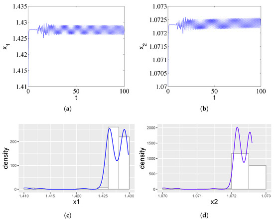
Figure 2. Stable periodic oscillations arising from a Fold–Hopf bifurcation in system (1) for a supercritical time delay ${\tau }_4=0.5>{\tau }_0=0.48$. (a) Time series of the ampicillin-resistant population ($x_1$) exhibiting sustained, large-amplitude oscillations. (b) Corresponding dynamics of the chloramphenicol-resistant population ($x_2$) showing synchronous periodic behavior. The out-of-phase growth patterns reflect temporal segregation in cross-protection activities, where one strain deactivates its target antibiotic earlier, facilitating the other’s proliferation. (c,d) The nontrivial, crater-shaped probability density functions for $x_1$ and $x_2$ statistically confirm the emergence of a stable limit cycle, characterizing the persistent oscillatory coexistence observed in experimental studies.

Due to the randomness of the population or challenging environmental conditions, drug-resistant populations not only interact with antibiotics but are also associated with random disturbances. We consider here the effects of noise in the cross-protection model with numerical simulations. We introduce Gaussian white noise $\xi \left(t\right)$ with intensity $\sigma$ into the first equation of the deterministic system (1). We try to understand whether the stability of the system is consistent with that of the deterministic system when noise is added. We can observe irregular spiking behaviors in Figure 3; noise has a profound impact on the population dynamics.

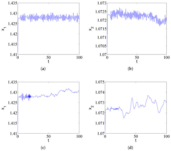
Figure 3. Impact of environmental noise ($\sigma =0.0008$) on population dynamics under different time delay conditions. (a,b) For ${\tau }_4=0.46<{\tau }_0$, Gaussian white noise induces irregular spiking behavior around the deterministic equilibrium, mimicking stochastic population fluctuations in realistic environments. (c,d) For ${\tau }_4=0.5>{\tau }_0$, noise perturbs the inherent limit cycle, causing random variations in oscillation amplitude and phase. These results demonstrate that environmental stochasticity can profoundly alter population trajectories, potentially triggering transient outbreaks even in parameter regions predicted to be stable by deterministic models, with implications for antibiotic treatment efficacy in noisy biological systems.

The numerical results presented in Figure 1, Figure 2 and Figure 3 provide compelling validation of the theoretical framework developed in Section 2. Specifically, the transition from asymptotic stability (${\tau }_4=0.46<{\tau }_0$) to sustained oscillations (${\tau }_4=0.5>{\tau }_0$) confirms the Fold–Hopf bifurcation predicted by our characteristic equation analysis. The emergence of limit cycle oscillations aligns quantitatively with the 3-day period and large-amplitude variations observed experimentally in [15], while the probability density functions offer statistical confirmation of the underlying deterministic dynamics. Furthermore, the noise-induced irregular spiking behaviors demonstrate how environmental stochasticity interacts with the intrinsic bifurcation structure, providing a more realistic representation of natural microbial communities. This tight integration of theoretical prediction and numerical verification establishes a comprehensive understanding of how time-delayed cross-protection generates the rich dynamical behaviors observed in experimental studies.

3.2. Parameter Sensitivity Analysis

The sensitivity analysis presented herein, which partitions the system’ s dynamics into subcritical (${\tau }_4=0.23$), critical (${\tau }_4=0.48$), and supercritical (${\tau }_4=0.8$) regimes based on the time delay ${\tau }_4$, provides a nuanced and state-dependent understanding of parametric influence. This approach, grounded in bifurcation theory, is implemented via a one-parameter-at-a-time method: systematically varying the growth rates ${\gamma }_1^R$ (5–9) and ${\gamma }_2^R$ (0.8–1.8) across 50 gradients while holding other parameters at their calibrated baseline values. The oscillatory amplitudes of $x_1$ and $x_2$, quantified as (max − min)/2 from steady-state solutions, are visualized on both linear and logarithmic scales to elucidate both absolute and relative changes.

As a critical reference point for assessing the specific role of time delays, Figure 4 illustrates the parameter sensitivity in the subcritical regime (${\tau }_4<{\tau }_0$), where the system exhibits damped oscillations converging toward a stable equilibrium. In this regime, the regulatory effects of both ${\gamma }_1^R$ and ${\gamma }_2^R$ on oscillation amplitudes are markedly suppressed due to the dominant damping effects that constrain population fluctuations and limit the transmission of interspecies competition dynamics.

Figure 4. Parameter sensitivity in the subcritical regime (${\tau }_4<{\tau }_0$). In this regime, characterized by damped oscillations converging to a stable equilibrium, the influence of growth rate parameters on oscillation amplitudes is significantly attenuated. (a,b) As ${\gamma }_1^R$ increases, the amplitude of $x_1$ shows only a modest linear rise, while the amplitude of $x_2$ remains minimal with no appreciable change. (c,d) Similarly, variations in ${\gamma }_2^R$ produce only negligible effects on both $x_1$ and $x_2$ amplitudes, with $x_2$ exhibiting a faint upward trend and $x_1$ maintaining a nearly constant level. The logarithmic-scale plots further confirm this weak sensitivity pattern, underscoring how damping effects effectively suppress population fluctuations and impede the propagation of competitive interactions through the system.

The parametric sensitivity undergoes a dramatic transformation at the critical regime (${\tau }_4={\tau }_0$), as depicted in Figure 5. Positioned precisely at the Fold–Hopf bifurcation threshold where the equilibrium loses stability, the system exhibits maximized sensitivity to parameter variations. This critical state significantly amplifies even minor parametric perturbations, markedly enhancing the transmission efficiency of interspecies competition and thereby activating the full regulatory potential of growth parameters on oscillation amplitudes.

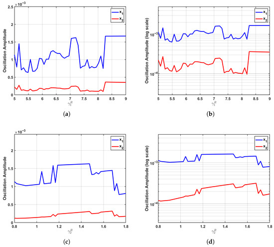
Figure 5. Enhanced parameter sensitivity at the critical regime (${\tau }_4={\tau }_0$). At the Fold–Hopf bifurcation point, where system stability is lost, parametric sensitivity reaches its maximum. (a,b) Increasing ${\gamma }_1^R$ induces a pronounced nonlinear amplification of the $x_1$ oscillation amplitude, while $x_2$ exhibits a clearly discernible upward trend despite maintaining relatively low amplitude levels. (c,d) Variations in ${\gamma }_2^R$ drive a substantial nonlinear increase in the $x_2$ amplitude, accompanied by a slight reduction in the $x_1$ amplitude. The logarithmic-scale visualizations reveal steeper response curves for both populations, demonstrating how the bifurcation point dramatically amplifies parametric perturbations and maximizes the regulatory efficacy of growth parameters through enhanced transmission of competitive interactions.

In the supercritical regime (${\tau }_4>{\tau }_0$), as presented in Figure 6, the system transitions into a stable limit cycle characterized by sustained oscillations and exhibits what we term “specific sensitivity”. The established limit cycle provides a stable environment for proliferative fluctuations of the corresponding population, while simultaneously solidifying the dominance patterns formed through interspecies competition, thereby attenuating parameter regulation on the amplitude of the non-corresponding population.

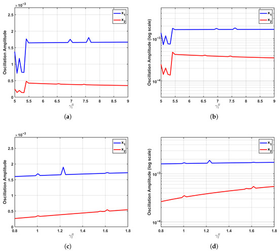
Figure 6. Specific sensitivity patterns in the supercritical regime (${\tau }_4>{\tau }_0$). Within the stable limit cycle regime of sustained oscillations, the system exhibits a distinctive specific sensitivity pattern. (a,b) Increasing ${\gamma }_1^R$ triggers a substantial nonlinear surge in the oscillation amplitude of $x_1$, while concurrently inducing a mild suppression in the amplitude of $x_2$. (c,d) Elevating ${\gamma }_2^R$ promotes a consistent monotonic nonlinear growth in the $x_2$ amplitude, whereas the $x_1$ amplitude remains largely unaffected and stable. Logarithmic-scale representations clearly demonstrate the emerging pattern of “significant amplification in the corresponding population with stability or attenuation in the other population”. This behavior arises because the limit cycle stabilizes proliferative fluctuations for each respective population while the solidified competitive dominance structure diminishes parametric control over the non-corresponding population’s amplitude.

In summary, our systematic sensitivity analysis reveals that the influence of growth parameters on oscillatory dynamics is profoundly state-dependent, governed by the system’s proximity to its bifurcation point. The transition from suppressed sensitivity in the subcritical regime, through dramatically amplified sensitivity at criticality, to the emergence of specific sensitivity within the supercritical limit cycle underscores a fundamental principle: parametric control is not intrinsic but is mediated by the underlying dynamical regime. This map of state-dependent sensitivity provides a critical theoretical framework for predicting system behavior and offers practical guidance for designing interventions—such as antibiotic treatment strategies—that can either exploit or avoid these highly sensitive operational windows.

4. Discussion and Future Perspectives

This study demonstrates, through rigorous theoretical analysis and numerical simulations, that a time-delay-induced Fold–Hopf bifurcation constitutes the intrinsic dynamical mechanism governing the transition from stable to oscillatory coexistence in microbial cross-protection systems. Beyond advancing our understanding of mutualistic microbial dynamics, these findings offer a theoretical foundation for optimizing clinical antibiotic treatment strategies.

4.1. Potential Clinical Implications of the Theoretical Findings

Our model identifies the timescale of biological feedback—captured by the delay $\tau$—as a key bifurcation parameter that governs system stability and oscillatory behavior. This perspective suggests a novel avenue for optimizing clinical combination therapy: This delay represents a potential therapeutic target that can be modulated to steer population dynamics toward a more treatable stable state. For instance, if adjustment agents (e.g., quorum-sensing inhibitors) could disrupt the speed at which bacteria coordinate their resistance mechanisms, effectively increasing the critical delay ${\tau }_c$, such modulation could shift the population from a resilient oscillatory state to a stable equilibrium, fundamentally improving treatment outcomes. Moreover, the model-derived critical thresholds provide a theoretical framework for tailoring personalized antibiotic dosing strategies, highlighting that the efficacy of combination therapy is governed not only by the drug combination itself but also by the temporal characteristics of inter-strain interactions.

4.2. Future Research Directions

Building on the present advances and limitations of microbial cross-protection population-dynamics models, future work will pursue three interlinked axes—model refinement, scope expansion, and translational deployment—to heighten both realism and practical impact.

Model refinement will transition frameworks from deterministic to spatio-stochastic representations. Deterministic frameworks will be extended to stochastic differential-equation models that embed environmental and demographic noise, enabling quantitative prediction of how random fluctuations reshape bifurcations and in vivo survival. Simultaneously, reaction–diffusion or agent-based formalizations will incorporate spatial heterogeneity to dissect how antibiotic gradients and cross-protection interact within structured habitats such as biofilms, illuminating the pathogenesis of chronic infections.

Scope expansion will shift the focus from dual-strain caricatures to multi-strain ecological networks. Research will move beyond simplified models to networks that integrate competition, cooperation, and cross-protection, thereby mirroring clinically relevant polymicrobial infections. This expanded scope is crucial for revealing how population-level resistance emerges and persists, offering a firmer theoretical basis for combating multidrug-resistant infections.

Translational deployment will bridge qualitative insight and quantitative forecasting through data-driven integration. This will be achieved through close collaboration with experimental microbiologists, leveraging high-resolution time-series data for rigorous parameter estimation and validation. The ultimate aim is to convert conceptual understanding into predictive tools that forecast treatment outcomes and directly inform the optimization of antibiotic therapies, thereby closing the loop between fundamental discovery and clinical practice.

5. Conclusions

This study constructs the first comprehensive theoretical framework for microbial cross-protection symbiosis and reveals the fundamental driver of its oscillatory coexistence: a delay-induced Hopf bifurcation. By deriving the exact critical delay ${\tau }_0$, we convert biological lag from a descriptive parameter into a quantitative predictor of the transition between steady and oscillatory states, providing a rigorous mechanistic explanation for previously reported population cycles. Direct numerical simulations confirm the bifurcation, while the characteristic crater-shaped probability density statistically validates the underlying deterministic dynamics. Further, we show how environmental noise interacts with the bifurcation structure to generate spike-like fluctuations that mirror real ecological variability, aligning theory with field observations. Shifting from phenomenological description to predictive capability, our framework supplies ${\tau }_0$ as an operational tool for forecasting community trajectories, bridges experimental microbiology and nonlinear dynamics, and offers a mathematical foundation for optimizing clinical antibiotic protocols and managing natural microbial ecosystems.

References

- Azam, F.; Malfatti, F. Microbial structuring of marine ecosystems. Nat. Rev. Microbiol. 2007, 5, 782–791. [Google Scholar] [CrossRef]
- Fierer, N. Embracing the unknown: Disentangling the complexities of the soil microbiome. Nat. Rev. Microbiol. 2017, 15, 579–590. [Google Scholar] [CrossRef]
- Arumugam, M.; Raes, J.; Pelletier, E.; Le Paslier, D.; Yamada, T.; Mende, D.R.; Fernandes, G.R.; Tap, J.; Bruls, T.; Batto, J.-M.; et al. Enterotypes of the human gut microbiome. Nature 2011, 473, 174–180. [Google Scholar] [CrossRef] [PubMed]
- Huttenhower, C.; Gevers, D.; Knight, R.; Abubucker, S.; Badger, J.H.; Chinwalla, A.T.; Creasy, H.H.; Earl, A.M.; FitzGerald, M.G.; Fulton, R.S.; et al. Structure, function and diversity of the healthy human microbiome. Nature 2012, 486, 207–214. [Google Scholar] [CrossRef] [PubMed]
- Falkowski, P.G.; Fenchel, T.; Delong, E.F. The microbial engines that drive Earth’s biogeochemical cycles. Science 2008, 320, 1034–1039. [Google Scholar] [CrossRef]
- Thompson, L.R.; Sanders, J.G.; McDonald, D.; Amir, A.; Ladau, J.; Lacey, K.J.; Prill, R.J.; Tripathi, A.; Gibbons, S.M.; Ackermann, G.; et al. A communal catalogue reveals Earth’s multiscale microbial diversity. Nature 2017, 551, 457–463. [Google Scholar] [CrossRef]
- Boucher, D.H.; James, S.; Keeler, K.H. The ecology of mutualism. Annu. Rev. Ecol. Syst. 1982, 13, 315–347. [Google Scholar] [CrossRef]
- Bronstein, J.L. Conditional outcomes in mutualistic interactions. Trends Ecol. Evol. 1994, 9, 214–217. [Google Scholar] [CrossRef] [PubMed]
- Bruno, J.F.; Stachowicz, J.J.; Bertness, M.D. Inclusion of facilitation into ecological theory. Trends Ecol. Evol. 2003, 18, 119–125. [Google Scholar] [CrossRef]
- Conlin, P.L.; Chandler, J.R.; Kerr, B. Games of life and death: Antibiotic resistance and production through the lens of evolutionary game theory. Curr. Opin. Microbiol. 2014, 21, 35–44. [Google Scholar] [CrossRef]
- Lee, H.H.; Molla, M.N.; Cantor, C.R.; Collins, J.J. Bacterial charity work leads to population-wide resistance. Nature 2010, 467, 82–85. [Google Scholar] [CrossRef] [PubMed]
- Meredith, H.R.; Srimani, J.K.; Lee, A.J.; Lopatkin, A.J.; You, L. Collective antibiotic tolerance: Mechanisms, dynamics and intervention. Nat. Chem. Biol. 2015, 11, 182–188. [Google Scholar] [CrossRef] [PubMed]
- Vega, N.M.; Gore, J. Collective antibiotic resistance: Mechanisms and implications. Curr. Opin. Microbiol. 2014, 21, 28–34. [Google Scholar] [CrossRef]
- Yurtsev, E.A.; Chao, H.X.; Datta, M.S.; Artemova, T.; Gore, J. Bacterial cheating drives the population dynamics of cooperative antibiotic resistance plasmids. Mol. Syst. Biol. 2013, 9, 683. [Google Scholar] [CrossRef] [PubMed]
- Yurtsev, E.A.; Conwill, A.; Gore, J. Oscillatory dynamics in a bacterial cross-protection mutualism. Proc. Natl. Acad. Sci. USA 2016, 113, 6236–6241. [Google Scholar] [CrossRef]
- May, R.M. Biological populations with nonoverlapping generations: Stable points, stable cycles, and chaos. Science 1974, 186, 645–647. [Google Scholar] [CrossRef]
- Kendall, B.E.; Briggs, C.J.; Murdoch, W.W.; Turchin, P.; Ellner, S.P.; McCauley, E.; Nisbet, R.M.; Wood, S.N. Why do populations cycle? A synthesis of statistical and mechanistic modeling approaches. Ecology 1999, 80, 1789–1805. [Google Scholar] [CrossRef]
- Kendall, B.E.; Prendergast, J.; Bjornstad, O.N. The macroecology of population dynamics: Taxonomic and biogeographic patterns in population cycles. Ecol. Lett. 1998, 1, 160–164. [Google Scholar] [CrossRef]
- Lindström, J.; Ranta, E.; Kaitala, V.; Lindén, H. The clockwork of Finnish tetraonid population dynamics. Oikos 1995, 72, 185–194. [Google Scholar] [CrossRef]
- Turchin, P. Chaos and stability in rodent population dynamics: Evidence from non-linear time-series analysis. Oikos 1993, 68, 167–172. [Google Scholar] [CrossRef]
- Ellner, S.; Turchin, P. Chaos in a noisy world: New methods and evidence from time-series analysis. Am. Nat. 1995, 145, 343–375. [Google Scholar] [CrossRef]
- Hassell, M.P.; Lawton, J.H.; May, R. Patterns of dynamical behaviour in single-species populations. J. Anim. Ecol. 1976, 45, 471–486. [Google Scholar] [CrossRef]
- Hale, J.K. Retarded functional differential equations: Basic theory. In Theory of Functional Differential Equations; Springer: New York, NY, USA, 1977; pp. 36–56. [Google Scholar] [CrossRef]
- Faria, T.; Magalhães, L.T. Restrictions on the possible flows of scalar retarded functional differential equations in neighborhoods of singularities. J. Dyn. Differ. Equ. 1996, 8, 35–70. [Google Scholar] [CrossRef]
Disclaimer/Publisher’s Note: The statements, opinions and data contained in all publications are solely those of the individual author(s) and contributor(s) and not of MDPI and/or the editor(s). MDPI and/or the editor(s) disclaim responsibility for any injury to people or property resulting from any ideas, methods, instructions or products referred to in the content. |
© 2025 by the authors. Licensee MDPI, Basel, Switzerland. This article is an open access article distributed under the terms and conditions of the Creative Commons Attribution (CC BY) license (https://creativecommons.org/licenses/by/4.0/).