Adaptive Sparse Clustering of Mixed Data Using Azzalini-Encoded Ordinal Variables

Abstract

In this paper, we propose a novel sparse clustering method designed for high-dimensional mixed-type data, integrating Azzalini’s score-based encoding for ordinal variables. Our approach aims to retain the inherent nature of each variable type—continuous, ordinal, and nominal—while enhancing clustering quality and interpretability. To this end, we extend classical distance metrics and adapt the Davies–Bouldin Index (DBI) to better reflect the structure of mixed data. We also introduce a weighted formulation that accounts for the distinct contributions of variable types in the clustering process. Empirical results on simulated and real-world datasets demonstrate that our method consistently achieves better separation and coherence of clusters compared to traditional techniques, while effectively identifying the most informative variables. This work opens promising directions for clustering in complex, high-dimensional settings such as marketing analytics and customer segmentation.

1. Introduction

Unsupervised clustering plays a central role in modern data analysis, helping to uncover underlying patterns in complex datasets. Yet, most classical clustering algorithms assume that all variables share the same type. In practice, however, many real-world datasets—such as those in marketing, healthcare, or social sciences—combine multiple variable types: continuous measurements (e.g., age, income), nominal categories (e.g., gender, product type), and ordinal ratings (e.g., education level, satisfaction score). This mixture of variable types presents a major challenge, since conventional clustering methods are not designed to handle such heterogeneity or to respect the structural properties specific to each variable type [1,2]. A comprehensive overview of these challenges in mixed-data clustering is provided by [3], which highlights the limitations of distance-based and model-based approaches when dealing with heterogeneous attributes.

Among these variable types, ordinal variables are particularly delicate to handle. They possess a natural order, but their categories do not have meaningful numerical distances. In many studies, ordinal variables are either treated as nominal—thereby discarding their order—or converted into arbitrary integer scales, which may create artificial patterns and distort distances. As emphasized by [4], preserving ordinality is crucial for maintaining the hierarchical information carried by ordered categories. When ordinal data are mishandled, cluster interpretability suffers, and the resulting partitions may fail to reflect the true relationships in the data, especially in high-dimensional settings with noisy or redundant features.

To overcome these issues, several approaches have been proposed for clustering mixed-type datasets. Sparse k-means [5] combines Euclidean distance for continuous variables with matching dissimilarities for categorical variables, while more sophisticated probabilistic models such as latent class clustering [6,7] and model-based clustering for mixed data [8] rely on distributional assumptions. Methods based on Gower’s distance [9] followed by hierarchical or PAM clustering [10] also remain popular. More recent advances include mixed-data clustering based on multiple correspondence analysis (MCA) [11,12] and sparse latent mixture models such as VarSelLCM [13]. However, these approaches either ignore ordinal structure, require strong parametric assumptions, or lack mechanisms for variable selection in high-dimensional settings.

To address these limitations, we introduce a new sparse clustering approach called DBI–SC–Azzalini, which extends the Davies–Bouldin Index (DBI) framework with adaptive dissimilarity measures tailored to each variable type. Building on recent advances in sparse clustering [5,14,15], our method integrates clustering and variable selection within a unified optimization framework. It employs distinct penalization schemes for continuous, ordinal, and nominal variables, enabling automatic identification of the most relevant features in high-dimensional mixed data.

A key innovation of our approach lies in its treatment of ordinal variables. Instead of using traditional dummy encoding—which destroys ordinal structure—we leverage the quantile-based score transformation of [16]. This encoding maps ordinal categories to continuous scores while preserving their order and approximate spacing, thereby allowing ordinal variables to be seamlessly integrated into Euclidean distance calculations. This overcomes well-known limitations of treating ordinal data as either numeric or nominal, and it avoids strong model assumptions commonly used in ordinal latent variable models [17,18].

Our DBI–SC–Azzalini method computes variable-specific contributions using a modified Davies–Bouldin Index, balancing between-cluster separation and within-cluster compactness. For continuous variables, we use the squared Euclidean distance; for nominal variables, we apply co-occurrence-based dissimilarities [19]; and for ordinal variables, the Azzalini score allows for metric comparison while preserving ordinality. Each variable type is penalized independently within a sparsity-constrained optimization setting to identify the most relevant features.

This strategy yields multiple benefits:

• Non-parametric robustness, since DBI–SC–Azzalini does not assume a particular probability model [20];
• Scalability, making it suitable for modern large-scale datasets;
• Interpretability, by retaining only informative variables and identifying those driving cluster structure;
• Flexibility, adapting to diverse data types without requiring user-defined weights or parametric assumptions.

The main contributions of this paper are as follows:

• Novel ordinal encoding: We adapt Azzalini’s quantile-based score transformation [16] for clustering, preserving ordinality in Euclidean space.
• Type-adaptive distances: We integrate continuous (Euclidean), ordinal (Azzalini scores), and nominal (co-occurrence) distances within a unified sparse clustering framework.
• Theoretical guarantees: We establish screening consistency for mixed-type data, ensuring recovery of informative variables.
• Empirical validation: Through simulations and a real bank marketing application, we demonstrate superior clustering and variable-selection performance.

We provide theoretical guarantees by establishing the screening consistency of DBI–SC–Azzalini: the ability to asymptotically recover all informative variables while excluding noise. This property remains rare among existing mixed-data clustering methods [12].

To validate the proposed method, we conduct extensive simulation studies (Section 5), demonstrating improved clustering accuracy and feature-selection quality compared with Sparse k-means [5], VarSelLCM [13], and PAM clustering based on Gower’s dissimilarity [21]. We further apply DBI–SC–Azzalini to a real-world bank marketing dataset (Section 6), where it identifies meaningful clusters while preserving interpretability and reducing dimensionality.

The remainder of the article is organized as follows. Section 2 introduces the DBI–SC–Azzalini methodology, including score transformations, dissimilarity measures, and optimization. Section 4 presents theoretical results on screening consistency. Section 5 reports simulation experiments comparing the proposed method with existing approaches. Section 6 demonstrates its practical utility through a real-data application. Section 7 concludes with final remarks and future directions.

2. Methodology

Let us consider a dataset composed of n observations, which can be grouped into K clusters. For each observation i ($1\le i\le n$), we observe p continuous variables, r ordinal variables, and q nominal variables, represented by the vector $X_i={(x_{i1},\dots ,x_{ip+r+q})}^{\top }$. By convention, the first p variables ($x_{i1}$ to $x_{ip}$) are continuous, the next r variables ($x_{ip+1}$ to $x_{ip+r}$) are ordinal, and the final q variables ($x_{ip+r+1}$ to $x_{ip+r+q}$) are nominal. The set of variables for all n observations is denoted $X={(X_1,\dots ,X_n)}^{\top }$. For each variable j ($1\le j\le p+r+q$), we define a value space ${\mathcal{X}}_j$. For continuous variables ($j=1,\dots ,p$), this space is ${\mathcal{X}}_j=\mathbb{R}$. For ordinal variables ($j=p+1,\dots ,p+r$), it is ${\mathcal{X}}_j=\{1,\dots ,M_j\}$, where $M_j$ is the number of ordered levels of the j-th ordinal variable. Finally, for nominal variables ($j=p+r+1,\dots ,p+r+q$), the space is ${\mathcal{X}}_j=\{1,\dots ,L_j\}$, where $L_j$ is the number of levels of the j-th nominal variable.

The objective of this study is to group the n observations into K clusters using the observable variable X. For this, it is essential to measure dissimilarity between any two observations. As the data include mixed-type variables (continuous, ordinal, and nominal), we define distance measures adapted to each variable type.

First, we assume that continuous variables have been standardized (zero mean and unit variance). The dissimilarity between two observations for a continuous variable is measured using the Euclidean distance. Thus, for the j-th continuous variable, the distance between observations i and $i^{\prime }$ is given by ${(x_{ij}-x_{i^{\prime }j})}^2$.

2.1. Ordinal Variables

The use of ordered factors presents several challenges due to their inherently qualitative but ordered nature. In this context, the methodology proposed by [16] allows for an optimal transformation of these variables to simplify their interpretation while preserving, or even improving, the quality of fit compared to classical approaches.

The method begins by assigning non-equidistant scores to each level of an ordinal factor, based on a transformation of the quantiles of a flexible parametric distribution. Let X be an ordinal factor with K levels $\{1,\dots ,K\}$. The initially equidistant scores are given by

$$u_k={\displaystyle \frac{k}{K+1}},k=1,2,\dots ,K.$$

These scores are then transformed using the quantile function Q of a parametric distribution P:

$$q_k=Q(u_k;\theta ),$$

where $\theta$ is a vector of parameters characterizing the chosen distribution. The considered distributions include flexible families such as Tukey’s g-and-h distribution and Johnson’s SU distribution, which are particularly suitable for capturing the complexity of ordinal data.

SU Distribution (Johnson):

$$Y=sinh\left({\displaystyle \frac{Z-\gamma }{\delta }}\right)$$

• $\gamma$: Location parameter;
• $\delta >0$: Scale parameter.

g-and-h Distribution (Tukey):

$$Y=\left\{\begin{array}{cc}Z{e}^{h{Z}^2/2}\hfill & g=0\hfill \\ {\displaystyle \frac{e^{gZ}-1}{g}}{e}^{h{Z}^2/2}\hfill & g\ne 0\hfill \end{array}\right.$$

• g controls skewness;
• h controls tail heaviness.

sinh-arcsinh Distribution (Jones & Pewsey):

$$Y=sinh\left(\delta ·\mathrm{arcsinh}\left(Z\right)+\epsilon \right)$$

• $\epsilon$: Skewness parameter;
• $\delta >0$: Tail parameter.

Once the $q_k$ scores are obtained for each ordinal factor, they are integrated into the Euclidean distance calculation as follows:

$$d(i,j)=\sum _{k=p+1}^{p+r}{(q_{ik}-q_{jk})}^2,$$

where $q_{ik}$ represents the transformed values of the ordinal variables for individual i.

2.2. Nominal Variables

Nominal variables are converted into binary indicators (dummy coding):

$$X_{ij}=\left\{\begin{array}{cc}1\hfill & \mathrm{if}\mathrm{observation}i\mathrm{belongs}\mathrm{to}\mathrm{category}j\hfill \\ 0\hfill & \mathrm{otherwise}\hfill \end{array}\right.$$

Each category is represented by a binary column, allowing these variables to be effectively integrated into clustering algorithms.

2.3. Distances for Mixed Data

The overall distance between two observations is a weighted combination of distances calculated for continuous and ordinal variables. For continuous variables, we use the standard Euclidean distance, computed as the sum of squared differences. For ordinal variables, after transforming levels into scores using the method from [16], we also compute a Euclidean distance. The overall Euclidean distance is, thus,

$$d(i,j)=\sum _{k=1}^p{(x_{ik}-x_{jk})}^2+\sum _{k=p+1}^{p+r}{(q_{ik}-q_{jk})}^2$$

For nominal variables, we use the co-occurrence distance proposed by [19]. This distance measures the dissimilarity between two levels a and b of a categorical variable $X_j$ by considering the conditional co-occurrence probabilities with the levels of other categorical variables. Formally, the distance ${\delta }_{ab}\left(j\right)$ is defined as

$${\delta }_{ab}\left(j\right)=\sum _{j^{\prime }\in \{p+1,\dots ,p+q\}\setminus \left\{j\right\}}\sum _{l^{\prime }=1}^{L_{j^{\prime }}}max\left\{\mathbb{P}(X_{j^{\prime }}=l^{\prime }\mid X_j=a),\mathbb{P}(X_{j^{\prime }}=l^{\prime }\mid X_j=b)\right\}.$$

Explanation of the notation:

• $j^{\prime }$: Index of other categorical variables in the dataset.
• $L_{j^{\prime }}$: Number of levels of categorical variable $X_{j^{\prime }}$.
• $\mathbb{P}(X_{j^{\prime }}=l^{\prime }\mid X_j=a)$: Conditional probability that variable $X_{j^{\prime }}$ takes level $l^{\prime }$ given that $X_j$ takes level a.

• Probability space and events.

Let $(\Omega ,\mathcal{F},\mathbb{P})$ denote the probability space, where $\Omega$ is the set of all observations, $\mathcal{F}$ is the sigma-algebra of events, and $\mathbb{P}$ is the probability measure. For a level a of $X_j$, define the event as

$$A=\{\omega \in \Omega :X_j\left(\omega \right)=a\}.$$

Similarly, for another level b of $X_j$, define $B=\{\omega \in \Omega :X_j\left(\omega \right)=b\}$. Then, the conditional probability of $X_{j^{\prime }}$ being at level $l^{\prime }$ given that $X_j$ is at level a is

$$\mathbb{P}(X_{j^{\prime }}=l^{\prime }\mid X_j=a)=\mathbb{P}(\{\omega \in \Omega :X_{j^{\prime }}\left(\omega \right)=l^{\prime }\}\mid A),$$

which can be estimated empirically from the observed data as

$$\widehat{\mathbb{P}}(X_{j^{\prime }}=l^{\prime }\mid X_j=a)={\displaystyle \frac{\mathrm{Number}\mathrm{of}\mathrm{observations}\mathrm{with}{X}_j=a\mathrm{and}{X}_{j^{\prime }}=l^{\prime }}{\mathrm{Number}\mathrm{of}\mathrm{observations}\mathrm{with}{X}_j=a}}.$$

This formalism ensures that the co-occurrence distance is rigorously defined in terms of the probability space and events corresponding to each level of the categorical variables.

This formulation emphasizes that the distance is computed based on conditional probabilities associated with the levels of categorical variables. It allows us to interpret the distance in terms of probabilistic similarity between observations.

To make distances comparable across different categorical variable levels, we normalize these distances to the interval $[0,1]$. The normalized distance between two levels a and b of a categorical variable j is calculated as

$${\tilde{\delta }}_{ab}\left(j\right)=1-{\displaystyle \frac{{\delta }_{ab}\left(j\right)}{q-1}},$$

where ${\delta }_{ab}\left(j\right)$ is the raw distance between levels a and b, and q is the total number of levels of the categorical variable.

To perform variable selection, it is essential to measure the dispersion of individual variables between and within clusters. Let $d_{i{i}^{\prime },j}$ be the dissimilarity measure between two observations i and $i^{\prime }$ for variable j. This dissimilarity can be defined as

$$d_{i{i}^{\prime },j}=\left\{\begin{array}{cc}{(x_{ij}-x_{i^{\prime }j})}^2,\hfill & 1\le j\le p,\hfill \\ {(q_{ik}-q_{jk})}^2,\hfill & p+1\le j\le p+r,\hfill \\ \sum _{l=1}^{L_j}\sum _{l^{\prime }\ne l}{\tilde{\delta }}_{l{l}^{\prime }}\left(j\right)I(x_{ij}=l)I(x_{i^{\prime }j}=l^{\prime }),\hfill & p+r+1\le j\le p+r+q,\hfill \end{array}\right.$$

where $I(·)$ is the indicator function.

Furthermore, for a cluster k where $1\le k\le K$, let $C_k$ be the set of observations in cluster k and $n_k$ be the number of observations in $C_k$. The within-cluster dispersion for cluster k and variable j is defined as

$${\sigma }_{k,j}\left(C\right)={\displaystyle \frac{{\sum }_{i,i^{\prime }\in C_k}{d}_{i{i}^{\prime },j}}{n_k^2-n_k}}.$$

For two clusters k and $k^{\prime }$, the between-cluster dispersion for variable j is given by

$${\theta }_{k{k}^{\prime },j}\left(C\right)={\displaystyle \frac{{\sum }_{i\in C_k}{\sum }_{i^{\prime }\in C_{k^{\prime }}}{d}_{i{i}^{\prime },j}}{n_k{n}_{k^{\prime }}}}.$$

These measures allow quantification of the compactness and separation of clusters with respect to each variable, thereby providing a basis for optimization in the DBI-SC-Azzalini framework.

3. Sparse Clustering Framework

The original sparse clustering framework, proposed by [5], can be expressed as follows:

$$\underset{\mathbf{w},\Theta \in D}{max}\left\{\sum _{j=1}^p{w}_{j}f(X_j,\Theta )\right\}$$

subject to the constraints

$${\parallel \mathbf{w}\parallel }_2^2\le 1,{\parallel \mathbf{w}\parallel }_1\le s,w_j\ge 0,\forall 1\le j\le p,$$

where

• $w_j$ is a weight associated with variable j.
• $1\le s\le \sqrt{p}$ is a tuning parameter controlling sparsity.
• $f(X_j,\Theta )$ is a function measuring the contribution of variable j to the clustering.
• ${\parallel \mathbf{w}\parallel }_2^2={\sum }_j{w}_j^2$ is the squared Euclidean norm.
• ${\parallel \mathbf{w}\parallel }_1={\sum }_j\left|w_j\right|$ is the L1 norm (sum of absolute values).

Optimization Problem for DBI-SC-Azzalini

The global distance between two observations i and $i^{\prime }$, denoted $d(X_i,X_{i^{\prime }})$, combines dissimilarity measures for continuous and categorical variables with specific weights:

$$\begin{array}{c}d(X_i,X_{i^{\prime }})=\underset{\mathrm{Weighted}\mathrm{distance}\mathrm{for}\mathrm{continuous}\mathrm{variables}}{\underbrace{\sum _{j_1=1}^p{w}_{j_1}{(x_{i{j}_1}-x_{i^{\prime }{j}_1})}^2}}+\underset{\mathrm{Weighted}\mathrm{distance}\mathrm{for}\mathrm{ordinal}\mathrm{variables}}{\underbrace{\sum _{j_1=p+1}^{p+r}{w}_{j_1}{(q_{i{j}_1}-q_{i^{\prime }{j}_1})}^2}}\hfill \\ \hfill +\underset{\mathrm{Weighted}\mathrm{distance}\mathrm{for}\mathrm{nominal}\mathrm{variables}}{\underbrace{\sum _{j_2=p+r+1}^{p+r+q}{z}_{j_2}\sum _{l=1}^{L_{j_2}}\sum _{l^{\prime }\ne l}{\tilde{\delta }}_{l{l}^{\prime }}\left(j_2\right)I(x_{i{j}_2}=l)I(x_{i^{\prime }{j}_2}=l^{\prime })}},\end{array}$$

where

• $w_j$ and $z_j$ are the weights associated with continuous, ordinal, and nominal variables, respectively.
• $w_j,z_j\ge 0$ for all j.

• Davies–Bouldin Index (DBI)

The original Davies–Bouldin Index, introduced in [22], is defined as

$$\mathrm{DBI}={\displaystyle \frac{1}{K}}\sum _{k=1}^K\underset{k^{\prime }\ne k}{max}\left({\displaystyle \frac{{\sigma }_k+{\sigma }_{k^{\prime }}}{d(c_k,c_{k^{\prime }})}}\right),$$

where

• K is the number of clusters.
• ${\sigma }_k$ is the average intra-cluster distance for cluster k.
• $d(c_k,c_{k^{\prime }})$ is the distance between the centers of clusters k and $k^{\prime }$.

A lower DBI indicates better clustering performance, as it reflects a balance between intra-cluster compactness and inter-cluster separation.

• Adjusted DBI for Variable Selection

To adapt the DBI to variable selection, the adjusted DBI for each variable j, proposed by [15], is defined as

$$\mathrm{adj}{\mathrm{DBI}}_j={\displaystyle \frac{1}{K}}\sum _{k=1}^K\underset{k^{\prime }\ne k}{max}\left({\displaystyle \frac{{\theta }_{k{k}^{\prime },j}}{{\sigma }_{k,j}+{\sigma }_{k^{\prime },j}}}\right),$$

where

• ${\theta }_{k{k}^{\prime },j}$ is the inter-cluster dispersion for variable j.
• ${\sigma }_{k,j}$ is the intra-cluster dispersion for variable j.

In this formulation, a higher $\mathrm{adj}{\mathrm{DBI}}_j$ indicates that variable j more effectively contributes to distinguishing between clusters.

• Objective Function for DBI-SC-Azzalini

The final objective function for the DBI–SC–Azzalini method summarizes the contributions of all variables:

$$\begin{array}{c}\underset{C_1,\dots ,C_K,\mathbf{w},\mathbf{z}}{max}\{\sum _{j_1=1}^p{w}_{j_1}\left({\displaystyle \frac{1}{K}}\sum _{k=1}^K\underset{k^{\prime }\ne k}{max}\left({\displaystyle \frac{{\theta }_{k{k}^{\prime },j_1}}{{\sigma }_{k,j_1}+{\sigma }_{k^{\prime },j_1}}}\right)\right)\hfill \\ +\sum _{j_1=p+1}^{p+r}{w}_{j_1}\left({\displaystyle \frac{1}{K}}\sum _{k=1}^K\underset{k^{\prime }\ne k}{max}\left({\displaystyle \frac{{\theta }_{k{k}^{\prime },j_1}}{{\sigma }_{k,j_1}+{\sigma }_{k^{\prime },j_1}}}\right)\right)\\ +\sum _{j_2=p+r+1}^{p+r+q}{z}_{j_2}\left({\displaystyle \frac{1}{K}}\sum _{k=1}^K\underset{k^{\prime }\ne k}{max}\left({\displaystyle \frac{{\theta }_{k{k}^{\prime },j_2}}{{\sigma }_{k,j_2}+{\sigma }_{k^{\prime },j_2}}}\right)\right)\},\end{array}$$

subject to

$${\parallel \mathbf{w}\parallel }_2^2\le {1,\parallel \mathbf{z}\parallel }_2^2\le {1,\parallel \mathbf{w}\parallel }_1\le s_w,{\parallel \mathbf{z}\parallel }_1\le s_z,w_{j_1},z_{j_2}\ge 0\forall j_1,j_2.$$

An important challenge in implementing the DBI–SC–Azzalini method is determining appropriate values for the number of clusters K and the tuning parameters $s_w$ and $s_z$, which control sparsity for (continuous/ordinal) and nominal variables. As previously noted, the original Davies–Bouldin Index (DBI) is widely used to evaluate clustering performance. In our framework, continuous variables are already numerical, and ordinal variables are transformed into numerical scores; therefore, their dissimilarities are computed using Euclidean distances. For this reason, continuous and ordinal variables naturally belong to the same variable group. Nominal variables, by contrast, are handled separately using the co-occurrence distance [19].

To properly evaluate clustering performance with mixed-type variables, we introduce a modified Davies–Bouldin Index (mDBI), defined as

$$\mathrm{mDBI}={\displaystyle \frac{1}{K}}\sum _{k=1}^K\left[{\displaystyle \frac{{\displaystyle \sum _{j_1=1}^{p+r}{w}_{j_1}\underset{k^{\prime }\ne k}{min}\left(\frac{{\sigma }_{k,j_1}+{\sigma }_{k^{\prime },j_1}}{{\theta }_{k{k}^{\prime },j_1}}\right)}}{{\displaystyle \sum _{j_1=1}^{p+r}{w}_{j_1}}}}+{\displaystyle \frac{{\displaystyle \sum _{j_2=p+r+1}^{p+r+q}{z}_{j_2}\underset{k^{\prime }\ne k}{min}\left(\frac{{\sigma }_{k,j_2}+{\sigma }_{k^{\prime },j_2}}{{\theta }_{k{k}^{\prime },j_2}}\right)}}{{\displaystyle \sum _{j_2=p+r+1}^{p+r+q}{z}_{j_2}}}}\right].$$

Here, ${\sigma }_{k,j}$ denotes the within-cluster dispersion of variable j in cluster k, and ${\theta }_{k{k}^{\prime },j}$ represents the distance between the centroids of clusters k and $k^{\prime }$ for variable j. The weights $w_{j_1}$ and $z_{j_2}$ correspond to the importance of continuous/ordinal and nominal variables, respectively.

The mDBI is used to simultaneously select the number of clusters K and the tuning parameters $s_w$ and $s_z$. A grid of candidate values for $\{K,s_w,s_z\}$ is evaluated, and the combination yielding the smallest mDBI value is selected as the optimal configuration.

4. Theoretical Consistency

Data Generation Model with Continuous, Ordinal, and Nominal Variables

For each observation $i\in \{1,\dots ,n\}$, let the data vector be split as follows:

• ${\mathbf{X}}_i^{\left(1\right)}=(x_{i1},\dots ,x_{ip})$: Continuous variables.
• ${\mathbf{X}}_i^{\left(2\right)}=(x_{ip+1},\dots ,x_{ip+r})$: Ordinal categorical variables.
• ${\mathbf{X}}_i^{\left(3\right)}=(x_{ip+r+1},\dots ,x_{ip+r+q})$: Nominal categorical variables.

To evaluate variable selection performance, we define the following terms:

• Signal variables: Variables that help distinguish between clusters.
• Noise variables: Variables that behave similarly across all clusters.

Let $p^{*}$, $r^{*}$, and $q^{*}$ denote the number of signal continuous, ordinal, and nominal variables, respectively. Without loss of generality, we assume signal variables are ordered first within each block. The remaining $p-p^{*}$, $r-r^{*}$, and $q-q^{*}$ variables are noise.

• Continuous Variables

Let ${\varphi }_i\in \{1,\dots ,K\}$ be the cluster label for observation i, drawn from a multinomial distribution with probabilities ${\pi }_1,\dots ,{\pi }_K$. Conditional on ${\varphi }_i=k$, the continuous part is generated as

$${\mathbf{X}}_i^{\left(1\right)}={\mathbf{z}}_{ik}\sim \mathcal{N}({\mathit{\mu }}_k,{\mathbf{I}}_p),$$

where ${\mathit{\mu }}_k=({\mu }_{k1},\dots ,{\mu }_{kp})$. For signal variables $j\le p^{*}$, we assume ${\mu }_{kj}\ne 0$, and there exists at least one j such that ${\mu }_{kj}\ne {\mu }_{k^{\prime }j}$ for $k\ne k^{\prime }$. For noise variables $j>p^{*}$, ${\mu }_{kj}=0$ for all k.

• Ordinal Variables

Let $x_{ip+j}\in \{1,\dots ,L_j^{\left(O\right)}\}$ for $j=1,\dots ,r$ be the jth ordinal variable. Conditional on ${\varphi }_i=k$, the variable is generated as

$$x_{ip+j}\sim \mathrm{Multinomial}(1;{\mathbf{p}}_{kj}^{\left(O\right)}),$$

where ${\mathbf{p}}_{kj}^{\left(O\right)}=(p_{kj}^{\left(O\right)}\left(1\right),\dots ,p_{kj}^{\left(O\right)}\left(L_j^{\left(O\right)}\right))$. For signal ordinal variables $j\le r^{*}$, there exists $k\ne k^{\prime }$ such that

$$\sum _{\ell =1}^{L_j^{\left(O\right)}}min\left(p_{kj}^{\left(O\right)}(\ell ),p_{k^{\prime }j}^{\left(O\right)}(\ell )\right)\le 0.4$$

is equivalent to requiring a total-variation separation of at least $0.6$ between the categorical distributions of two clusters. This guarantees a positive lower bound on the discriminative term ${\beta }_{kj}^{\left(2\right)}$, which is essential for establishing screening consistency. The use of a fixed positive separation constant follows established theoretical practice in high-dimensional clustering [5,15]. For noise variables $j>r^{*}$, $p_{kj}^{\left(O\right)}(\ell )=1/L_j^{\left(O\right)}$ for all ℓ and k.

• Nominal Variables

Let $x_{ip+r+j}\in \{1,\dots ,L_j^{\left(N\right)}\}$ for $j=1,\dots ,q$ be the jth nominal variable. Conditional on ${\varphi }_i=k$, it is drawn from

$$x_{ip+r+j}\sim \mathrm{Multinomial}(1;{\mathbf{p}}_{kj}^{\left(N\right)}),$$

where ${\mathbf{p}}_{kj}^{\left(N\right)}=(p_{kj}^{\left(N\right)}\left(1\right),\dots ,p_{kj}^{\left(N\right)}\left(L_j^{\left(N\right)}\right))$. For signal nominal variables $j\le q^{*}$, there exists $k\ne k^{\prime }$ such that

$$\sum _{\ell =1}^{L_j^{\left(N\right)}}min\left(p_{kj}^{\left(N\right)}(\ell ),p_{k^{\prime }j}^{\left(N\right)}(\ell )\right)\le 0.4.$$

For noise variables $j>q^{*}$, all levels are equiprobable: $p_{kj}^{\left(N\right)}(\ell )=1/L_j^{\left(N\right)}$ for all ℓ and k.

This setup ensures that signal variables (across types) provide discriminatory information between clusters, while noise variables contribute no class-specific variation.

Definition 1. 

Let $\widehat{\mathbf{w}}$ and $\widehat{\mathbf{z}}$ be the estimated weight vectors corresponding to the p continuous (and/or ordinal) variables and the q categorical variables, respectively. Define the support sets as follows:

$$\mathit{supp}\left(\widehat{\mathbf{w}}\right)=\left\{j|{\widehat{w}}_j\ne 0,1\le j\le p+r\right\},\mathit{supp}\left(\widehat{\mathbf{z}}\right)=\left\{j|{\widehat{z}}_j\ne 0,p+r+1\le j\le p+r+q\right\}.$$

We say that the estimated weight vectors obtained by the DBI-SC-Azzalini method possess the screening consistency property if the following holds as $n\to \infty$:

1. 

$P\left({\mathcal{S}}_w^{*}\subseteq supp\left(\widehat{\mathbf{w}}\right)\right)\to 1$;

2. 

$P\left({\mathcal{S}}_v^{*}\subseteq supp\left(\widehat{\mathbf{v}}\right)\right)\to 1$.

Here, ${\mathcal{S}}_w^{*}$ and ${\mathcal{S}}_v^{*}$ denote the sets of truly informative continuous/ordinal and categorical variables, respectively.

In other words, the DBI-SC-Azzalini method asymptotically includes all relevant variables in the estimated supports, thus achieving consistent variable screening.

• Notation

• Continuous/Ordinal Variables:

  $${\beta }_{kj}^{\left(1\right)}=\underset{k^{\prime }\ne k}{max}{\left({\mu }_{kj}-{\mu }_{k^{\prime }j}\right)}^2,$$

  where ${\mu }_{kj}$ is the mean of observations in cluster k for variable j.
• Nominal Variables:

  $${\beta }_{kj}^{\left(2\right)}=\underset{k^{\prime }\ne k}{max}{\displaystyle \frac{{\sum }_l{\sum }_{l^{\prime }}(p_{kj}\left(l\right)-p_{k^{\prime }j}\left(l\right))(p_{k^{\prime }j}\left(l^{\prime }\right)-p_{kj}\left(l^{\prime }\right)){\tilde{\delta }}_{l{l}^{\prime }}\left(j\right)}{{\sum }_l{\sum }_{l^{\prime }}{p}_{kj}\left(l\right)p_{kj}\left(l^{\prime }\right){\tilde{\delta }}_{l{l}^{\prime }}\left(j\right)+{\sum }_l{\sum }_{l^{\prime }}{p}_{k^{\prime }j}\left(l\right)p_{k^{\prime }j}\left(l^{\prime }\right){\tilde{\delta }}_{l{l}^{\prime }}\left(j\right)}},$$

  where $p_{kj}\left(l\right)$ is the relative frequency of modality l in cluster k for variable j, and ${\tilde{\delta }}_j^{l{l}^{\prime }}$ is a dissimilarity measure between modalities.
• The discriminative contributions of the variables satisfy the following bounds:

  $${\xi }_1=\underset{k,j}{min}{\beta }_{kj}^{\left(1\right)},{\xi }_2=\underset{k,j}{max}{\beta }_{kj}^{\left(1\right)},{\xi }_3=\underset{k,j}{min}{\beta }_{kj}^{\left(2\right)},{\xi }_4=\underset{k,j}{max}{\beta }_{kj}^{\left(2\right)}.$$

Theorem 1 

(Consistency of DBI-SC-Azzalini). Consider the following optimization problem associated with the DBI-SC-Azzalini method:

$$\begin{array}{c}\underset{C_1,\dots ,C_K,\mathbf{w},\mathbf{z}}{max}\{\sum _{j_1=1}^{p+r}{w}_{j_1}\left({\displaystyle \frac{1}{K}}\sum _{k=1}^K\underset{k^{\prime }\ne k}{max}\left({\displaystyle \frac{{\theta }_{k{k}^{\prime },j_1}}{{\sigma }_{k,j_1}+{\sigma }_{k^{\prime },j_1}}}\right)\right) \hfill \\ \hfill +\sum _{j_2=p+r+1}^{p+r+q}{z}_{j_2}\left({\displaystyle \frac{1}{K}}\sum _{k=1}^K\underset{k^{\prime }\ne k}{max}\left({\displaystyle \frac{{\theta }_{k{k}^{\prime },j_2}}{{\sigma }_{k,j_2}+{\sigma }_{k^{\prime },j_2}}}\right)\right)\}\end{array}$$

subject to the constraints

$${\parallel \mathbf{w}\parallel }_2^2\le {1,\parallel \mathbf{z}\parallel }_2^2\le {1,\parallel \mathbf{w}\parallel }_1\le s_w,{\parallel \mathbf{z}\parallel }_1\le s_z,w_j,z_j\ge 0\forall j.$$

Assume the tuning parameters $s_w$ and $s_z$ satisfy the following bounds:

$${\displaystyle \frac{{\sum }_{j=1}^{{(p+r)}^{*}}{\overline{\alpha }}_{w_j}-{\xi }_1{(p+r)}^{*}/4}{{\left({\sum }_{j=1}^{{(p+r)}^{*}}{\left({\overline{\alpha }}_{w_j}-{\xi }_1/4\right)}^2\right)}^{1/2}}}\le s_w\le {\displaystyle \frac{{\sum }_{j=1}^{{(p+r)}^{*}}{\overline{\alpha }}_{w_j}}{{\left({\sum }_{j=1}^{{(p+r)}^{*}}{\overline{\alpha }}_{w_j}^2\right)}^{1/2}}},$$

$${\displaystyle \frac{{\sum }_{j=1}^{q^{*}}{\overline{\alpha }}_{z_j}-{\xi }_3{q}^{*}/4}{{\left({\sum }_{j=1}^{q^{*}}{\left({\overline{\alpha }}_{z_j}-{\xi }_3/4\right)}^2\right)}^{1/2}}}\le s_z\le {\displaystyle \frac{{\sum }_{j=1}^{q^{*}}{\overline{\alpha }}_{z_j}}{{\left({\sum }_{j=1}^{q^{*}}{\overline{\alpha }}_{z_j}^2\right)}^{1/2}}}.$$

Here, ${\overline{\alpha }}_{w_j}$ and ${\overline{\alpha }}_{z_j}$ denote the average discriminative contributions of the continuous/ordinal and nominal variables, respectively.

Assume the following conditions hold:

• The number of informative continuous/ordinal variables ${(p+r)}^{*}$ and the number of informative nominal variables $q^{*}$ satisfy

  $${\left({(p+r)}^{*}\right)}^2\le {\displaystyle \frac{{\xi }_1^4}{2048{\xi }_2^2(1+{\xi }_2)ln\left(K\right)}},{\left(q^{*}\right)}^2\le {\displaystyle \frac{{\xi }_3^4}{2048{\xi }_4^2(1+{\xi }_4)ln\left(K\right)}}.$$
• The dimensionality of the problem grows moderately with the sample size n:

  $$ln(p+r+q)=o\left(n\right).$$

Then, the DBI-SC-Azzalini method is consistent in variable selection. Specifically, as $n\to \infty$, we have:

$$P\left(\{1,\dots ,{(p+r)}^{*}\}\subseteq supp\left(\mathbf{w}\right)\right)\to 1,P\left(\{p+r+1,\dots ,{(p+r+q)}^{*}\}\subseteq supp\left(\mathbf{z}\right)\right)\to 1.$$

That is, the method asymptotically includes all truly informative variables and excludes non-informative ones.

The detailed proof of Theorem 1 can be found in Appendix A.

5. Simulation Studies

To evaluate the effectiveness of the proposed DBI-SC-Azzalini method—which integrates variable-type-adaptive dissimilarities and Azzalini’s score encoding for ordinal variables—we conducted a series of simulation experiments on synthetic datasets. The goal was to assess the clustering accuracy, variable selection capability, and robustness of DBI-SC-Azzalini under diverse and realistic high-dimensional mixed-type settings. Each simulation scenario ($K=2,3,4$) was replicated 100 times with independently generated datasets and random initializations to ensure statistical reliability. Reported performance metrics correspond to the average results across these 100 replications.

• Cluster Structure

We simulated data from $K\in \{2,3,4\}$ clusters. For each cluster $k\in \{1,\dots ,K\}$, let $n_k$ denote the number of observations. The total sample size is $n={\sum }_{k=1}^K{n}_k$. We considered an imbalanced setting: one dominant cluster is defined as $n_1=0.4n$, and the remaining clusters share the rest: $n_2=\dots =n_K={\displaystyle \frac{0.6n}{K-1}}$.

Each observation comprises three types of variables:

• p continuous variables.
• r ordinal variables (coded using the Johnson SU distribution for all scenarios. In all simulation scenarios, the parameters were fixed at $\gamma =0$ and $\delta =1$.).
• q nominal variables.

We evaluated two configurations, $(p,r,q)\in \left\{\right(50,50,50),(100,100,100),(200,100,100\left)\right\}$, yielding high-dimensional mixed-type datasets.

We considered the folowing distributions for generating continuous data:

• Multivariate normal: A distribution consistent with the assumptions of our consistency theorem.
• p-generalized normal distribution: A flexible heavy-tailed distribution used in [23], with density

  $$f\left(x\right)={\displaystyle \frac{p^{1-1/p}}{2\sigma \Gamma (1/p)}}exp\left(-{\left|{\displaystyle \frac{x-\mu }{\sigma }}\right|}^p\right),$$

  where $\Gamma (·)$ denotes the Gamma function and $p>0$ controls tail heaviness.
  In all simulation experiments, we set

  $$p=0.7785,$$

  which produces heavier tails and higher kurtosis than the Gaussian case. This choice matches the parameterization implemented in our data-generating function (rpgnorm) and ensures comparability with the distributional settings used in [23].

The covariance matrix is generated using Joe’s method [24]. Variances are sampled from the interval $[1.5,2.5]$ to form a diagonal matrix D, and the final covariance matrix is given by $\Sigma =DRD$, where R is a random correlation matrix.

• Ordinal Variable Generation.

Ordinal variables take values in ordered sets with $L_j^{\left(O\right)}\in \{2,3,4,5\}$. For signal ordinal variables, cluster-specific probabilities $p_{kj}^{\left(O\right)}(\ell )$ are set so that

$$\sum _{\ell =1}^{L_j^{\left(O\right)}}min\left(p_{kj}^{\left(O\right)}(\ell ),p_{k^{\prime }j}^{\left(O\right)}(\ell )\right)\le 0.4.$$

These ordinal variables are encoded using Azzalini’s method before applying the clustering procedure. Noise ordinal variables follow uniform distributions over their respective levels in all clusters.

• Nominal Variable Generation.

Nominal variables have unordered categories with $L_j^{\left(N\right)}\in \{2,3,4,5\}$. Signal nominal variables are drawn from cluster-specific multinomial distributions with varying category probabilities. Noise nominal variables follow uniform multinomial distributions, with equal probabilities across all levels and clusters.

• Signal vs. Noise Variables.

Among all covariates, the following are designated as signal variables that define the cluster structure:

• 10 continuous variables;
• 10 ordinal variables;
• 10 nominal variables.

All others are noise variables and are drawn from their respective marginal distributions, uninformative of cluster membership.

• Evaluation Metrics.

To rigorously assess the clustering performance of our proposed DBI-SC-Azzalini method adapted to mixed-type high-dimensional data, we adopt a suite of well-established internal validation indices (

Table 1. Comparison of clustering methods for $K=2$, $K=3$, and $K=4$.

Method	$\mathit{K}=2$			$\mathit{K}=3$			$\mathit{K}=4$
	S	CH	mDBI	S	CH	mDBI	S	CH	mDBI
DBI_sc_Azzalini	0.1205	28.9208	2.3602	0.0322	11.8412	2.0566	0.0736	25.6553	1.9934
DBI_sc	0.0252	6.1432	3.3780	0.0163	5.8149	3.0110	0.0097	5.4423	2.9314
VarSelLCM	0.0250	6.0601	5.7148	0.0075	4.2375	7.1140	−0.0023	1.1475	13.2408
Sparse k-means	0.0247	5.9974	5.6866	0.0165	5.5042	8.6975	0.0111	5.8117	6.6063
SAS	0.0205	5.2144	6.0425	0.0148	5.3107	6.9147	0.0094	5.2984	7.0337
PAM	0.0019	1.4766	11.4412	−0.00171	1.4249	12.0516	−0.00570	1.2316	13.0981

Notes: S: Silhouette score (higher = better); CH: Calinski–Harabasz index (higher = better); mDBI: Davies–Bouldin Index (lower = better).

). These metrics evaluate different aspects of clustering quality, including compactness within clusters, separation between clusters, and the overall structure of the clustering solution. Specifically, we use the following two indices:

• Silhouette Score (S): This metric measures the similarity of each observation to its own cluster compared to other clusters. The Silhouette score ranges between $-1$ and 1, with higher values indicating better-defined and more cohesive clusters. It is particularly sensitive to both the intra-cluster compactness and the inter-cluster separation.
• Calinski–Harabasz Index (CH): Also known as the variance ratio criterion, this index is defined as the ratio of the between-cluster dispersion to the within-cluster dispersion. A higher CH value indicates that clusters are dense and well-separated, which is desirable for high-quality clustering. This metric is advantageous in high-dimensional contexts where variance plays a critical role in discrimination.

These two metrics are computed for each clustering solution under different simulation settings and for various numbers of clusters $K\in \{2,3,4\}$. We conducted comparisons between our method and competing clustering algorithms, including those not specifically tailored to handle mixed or high-dimensional data. For each evaluation metric and for each value of K, the best-performing method is emphasized in bold, allowing a clear comparison of effectiveness across techniques.

The use of these complementary evaluation criteria ensures a comprehensive validation of our method. While the Silhouette score provides a direct measure of clustering structure from an observation-wise perspective, the Calinski–Harabasz index captures the global variance structure. This pair of metrics allows us to assess both local and global clustering behaviors.

Empirical results from the simulation studies consistently show that the adaptive DBI-SC-Azzalini method outperforms other methods across all metrics, especially in complex scenarios involving high-dimensional, mixed-type data with both ordinal and nominal variables. The method achieves higher Silhouette and CH scores, and significantly lower DBI values, confirming its ability to identify compact, well-separated, and interpretable clusters. The observed superiority of DBI-SC-Azzalini underscores the importance of accounting for variable-specific structures and adapting dissimilarity measures accordingly.

In summary, the results confirm that the adaptive DBI-SC-Azzalini framework not only improves clustering accuracy but also enhances variable selection and interpretability by leveraging tailored dissimilarities and appropriate encoding schemes. These findings are further substantiated through the graphical representations and summary tables provided in the next sections.

The DBI_SC method based on Azzalini’s score encoding appears to be the best method in all cases, achieving the highest Calinski–Harabasz and Silhouette scores and the lowest DBI, indicating better separation and compactness of clusters.

Results Visualization with PCA

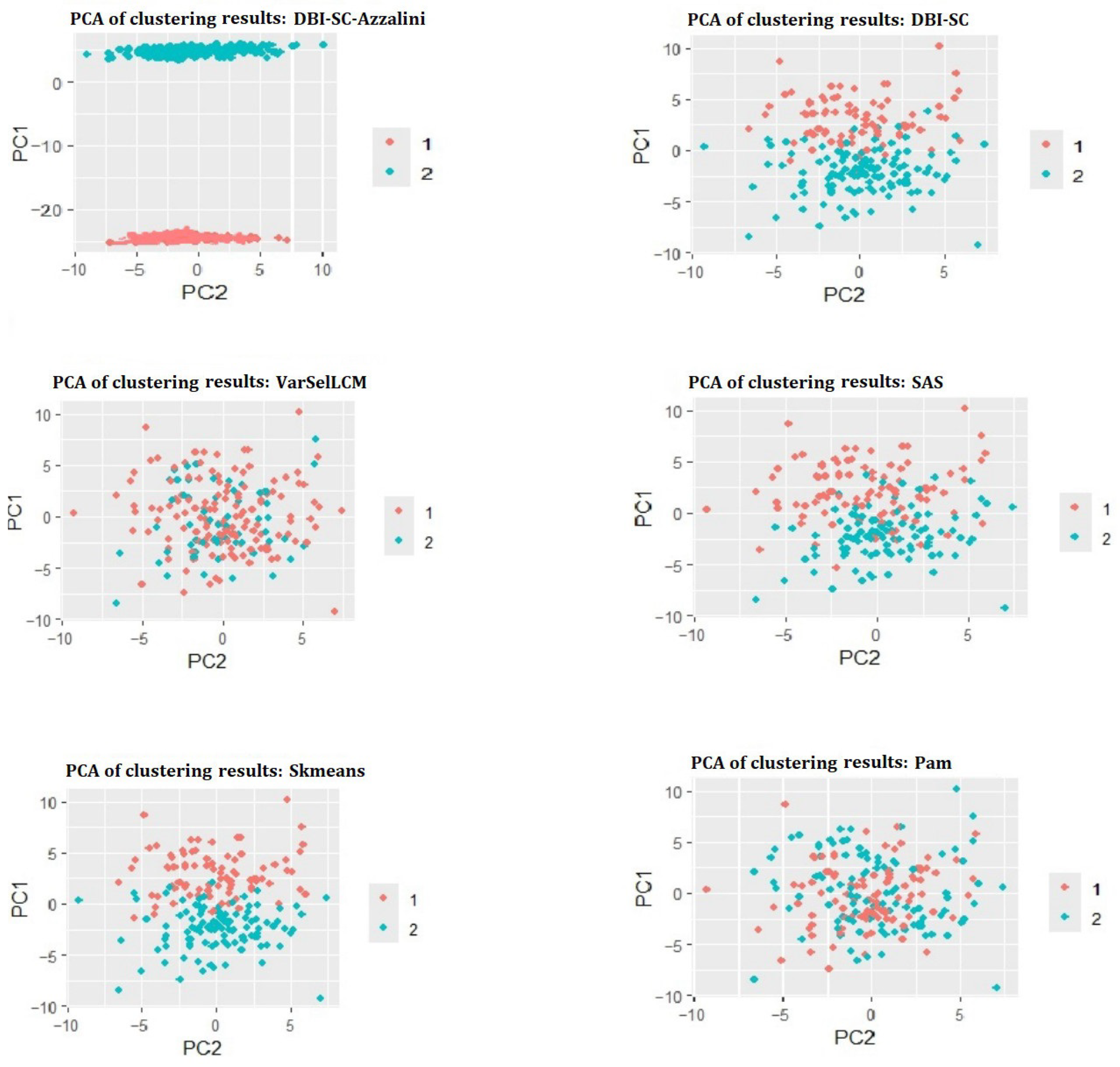
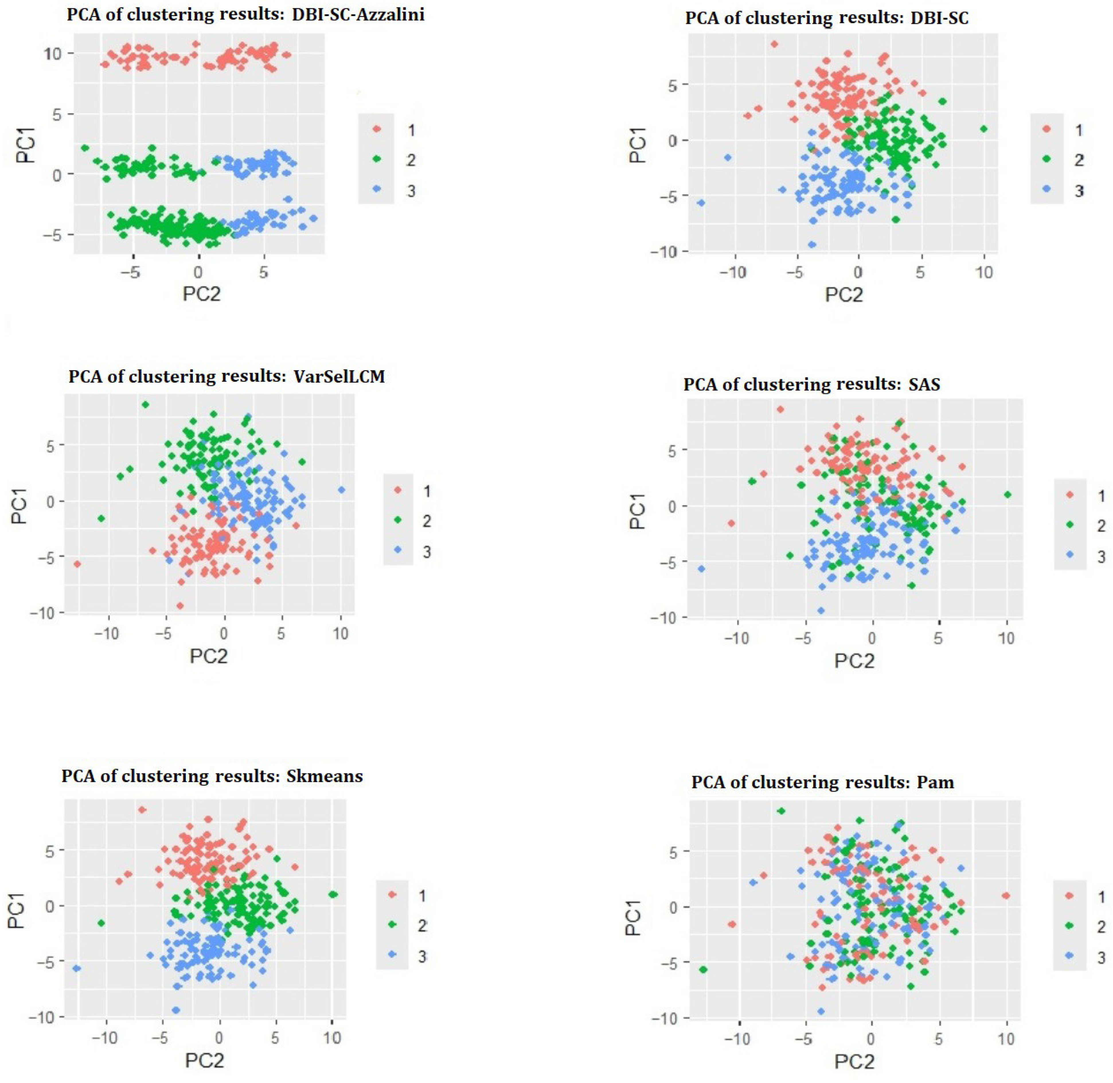
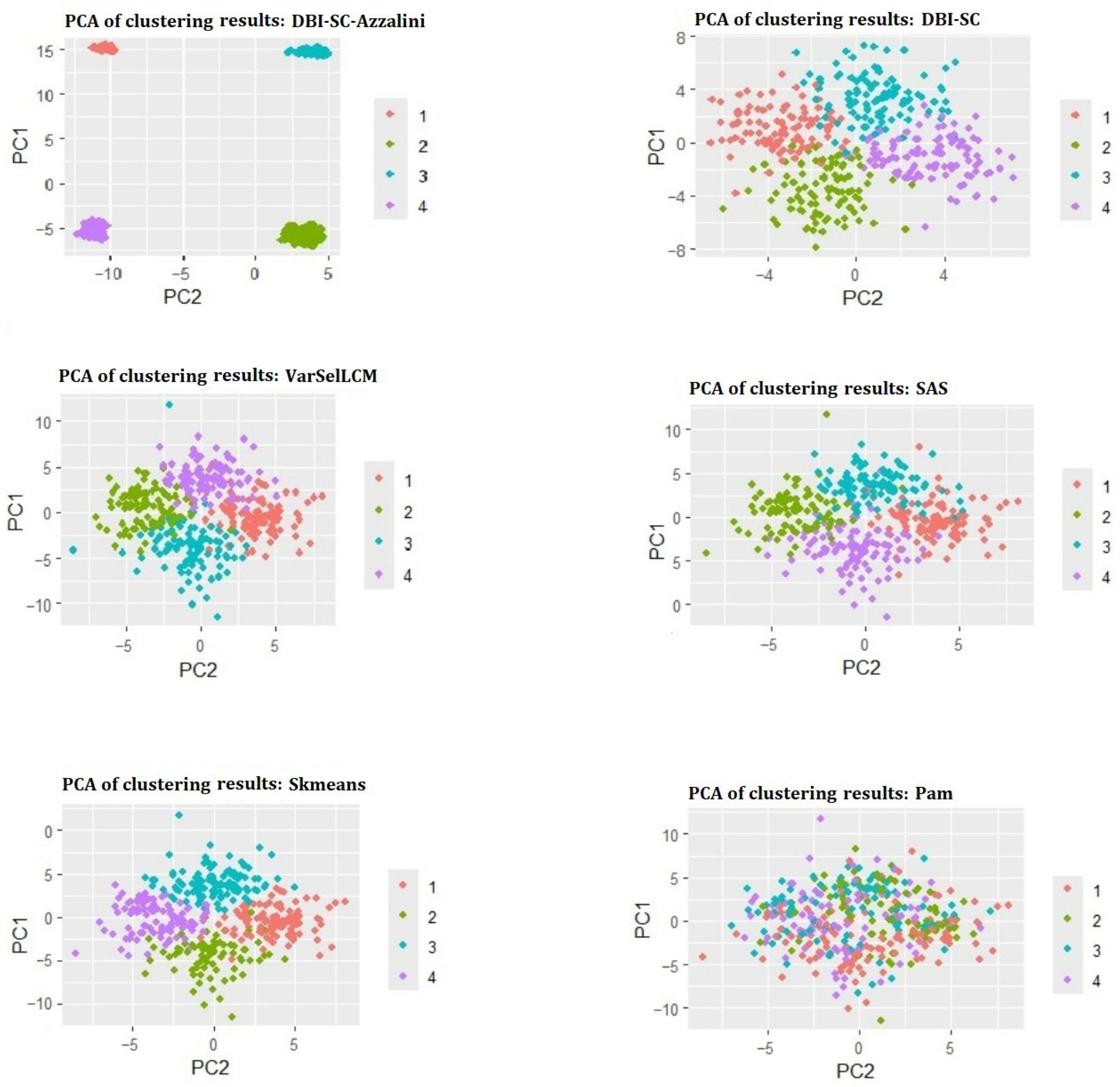
The following plots show the data projections from a random simulation onto the first two principal components (PCA) for each method and each value of K (Figure 1).

The PCA results for the three cases show better cluster separation, with less overlap when using score encoding for ordinal variables. This supports the previous results, confirming that the method based on Azzalini’s score produces more distinct and well-defined clusters (Figure 2).

The results obtained clearly show that the method based on Azzalini’s score offers better performance in terms of cluster separation compared to the use of dummy variables. The DBI, which measures clustering quality by considering both intra-cluster and inter-cluster distances, reveals that clusters formed using the Azzalini score method are not only better separated but also more coherent. This conclusion is reinforced by the PCA results, which show a clearer separation between clusters (Figure 3).

6. Real Data: Bank Marketing Dataset Description

The Bank Marketingdataset is a widely used public dataset for research in data analysis and direct marketing. It was created by Paulo Cortez (University of Minho) and Sérgio Moro (ISCTE-IUL) in 2012. The data relate to direct marketing campaigns of a Portuguese banking institution, where campaigns were primarily conducted via telephone calls. The aim of these campaigns was to determine whether a client would subscribe to a banking product, specifically a term deposit.

This dataset was described and analyzed in detail in the paper by [25] titled “Using Data Mining for Bank Direct Marketing: An Application of the CRISP-DM Methodology”. The paper was presented at the European Simulation and Modelling Conference (ESM’2011) in Guimarães, Portugal, in October 2011. The authors demonstrate the application of the CRISP-DM methodology (Cross-Industry Standard Process for Data Mining) to analyze and predict the success of direct marketing campaigns.

The data reflect interactions between the bank and its clients during the marketing campaigns. Multiple phone contacts were often necessary to determine whether a client would subscribe to the offered product (term deposit). The variables in the dataset cover demographic, socio-economic, and behavioral information about the clients, as well as details about the marketing campaigns.

The following table describes the variables included in the database (

Table 2. Description of variables in the Bank Marketing dataset.

Variable	Type	Description (Input Variables)
age	Numeric	Age of client
job	Categorical	Type of profession: “admin.”, “unknown”, “unemployed”, “management”, “housemaid”, “entrepreneur”, “student”, “blue-collar”, “self-employed”, “retired”, “technician”, “services”
marital	Categorical	Marital status: “married”, “divorced”, “single” (note: “divorced” includes widowed)
education	Ordinal	Level of education: “secondary”, “primary”, “tertiary”
default	Binary	Does the client have credit in default? (“yes”, “no”)
balance	Numeric	Average yearly balance in EUR
housing	Binary	Does the client have a housing loan? (“yes”, “no”)
loan	Binary	Does the client have a personal loan? (“yes”, “no”)
contact	Categorical	Type of communication: “unknown”, “telephone”, “cellular”
day	Numeric	Last day of contact in the month
month	Categorical	Last month of contact: “jan”, “feb”, “mar”, …, “nov”, “dec”
duration	Numeric	Duration of the last contact in seconds
campaign	Numeric	Number of contacts performed during this campaign (including the last contact)
pdays	Numeric	Number of days since the last contact from a previous campaign (−1 if the client was never contacted)
previous	Numeric	Number of contacts performed before this campaign
poutcome	Categorical	Outcome of the previous marketing campaign: “unknown”, “other”, “failure”, “success”

):

Continuous variables were normalized using Min–Max scaling. Categorical variables were encoded either via dummy coding or, for the ordinal variable education, via Azzalini’s score transformation in the DBI–SC–Azzalini method. Clustering performance was evaluated using the modified Davies–Bouldin Index (mDBI), the Silhouette coefficient, and the Calinski–Harabasz index.

• Ordinality Preservation: Numerical Evidence

Before comparing clustering methods, we provide numerical evidence that Azzalini’s score transformation preserves the ordinal structure of the education variable. The original education categories in the dataset are ordered as follows:

• [1] primary   secondary   tertiary

After applying the g-and-h Distribution transformation with parameters $(g=1,h=2)$, the transformed values become

• [1]  \textminus0.7731958   0.0000000   1.5178075

These values clearly maintain the original ordering and introduce meaningful spacing between education levels. This demonstrates that the score transformation replaces three redundant dummy variables with a single continuous variable that preserves ordinality, reduces dimensionality, and provides more informative distances between levels.

6.1. Clustering Performance Comparison

We compare six clustering methods on this dataset: (i) DBI–SC with dummy coding, (ii) DBI–SC–Azzalini, (iii) VarSelLCM, (iv) Sparse K-means, (v) SAS Clustering, (vi) PAM (Gower).

Higher Silhouette and Calinski–Harabasz scores indicate better separation, while lower mDBI values indicate more compact clusters (

Table 3. Comparison of clustering methods on the Bank Marketing dataset using the Silhouette coefficient, Calinski–Harabasz index, and modified Davies–Bouldin Index (mDBI).

Method	Silhouette	Calinski–Harabasz	mDBI
DBI–SC–Azzalini	0.0837	219.918	1.9989
DBI–SC	0.0334	86.2827	2.8247
VarSelLCM	0.0516	4.0448	14.8918
Sparse K-means	0.0083	23.2641	5.6752
SAS Clustering	0.0288	73.2638	9.0870
PAM	0.0876	189.1685	11.5213

).

The results reveal that DBI–SC–Azzalini achieves the lowest mDBI and the highest Calinski–Harabasz score, indicating a favorable balance between compactness and separation. Although its Silhouette value is modest, it remains among the best-performing methods. These results demonstrate that incorporating Azzalini’s score-based encoding enhances clustering performance on mixed data, particularly by preserving the ordinal structure of the education variable.

• Variable Selection Analysis

To investigate the variable-selection behavior of the two sparse clustering methods,

Table 4. Variable-selection results for DBI–SC and DBI–SC–Azzalini on the Bank Marketing dataset. A variable is marked as “Selected” when its associated weight is non-zero.

Variable	DBI–SC Weight	DBI–SC–Azzalini Weight
age	0.0027	0.0000
balance	0.0156	0.0000
day	0.9993	0.0000
duration	0.0007	0.0000
campaign	0.0164	0.0000
pdays	0.0271	0.0000
previous	0.0138	0.0000
job_admin.	0.0000	1.0000
job_blue-collar	0.0000	0.0000
job_entrepreneur	0.0000	0.0000
job_housemaid	0.0000	0.0000
job_management	0.0000	0.0000
job_retired	0.0000	0.0000
job_self-employed	0.0000	0.0000
job_services	0.0000	0.0000
job_student	0.0000	0.0000
job_technician	0.0000	0.0000
job_unemployed	0.0000	0.0000
job_unknown	0.0000	0.0000
marital_divorced	0.5856	0.0000
marital_married	0.5856	0.0000
marital_single	0.5856	0.0000
education_primary	0.0000	—
education_secondary	0.0000	—
education_tertiary	0.0000	—
education_score	—	0.3435
default_no	0.0000	0.9997
default_yes	0.8099	0.9997
housing_no	0.0000	0.0264
housing_yes	0.8099	0.0264
loan_no	0.0000	0.0000
loan_yes	0.0328	0.0000
contact_cellular	0.0328	0.0000
contact_telephone	0.0328	0.0000
contact_unknown	0.0000	0.0000
month_apr	0.0000	0.0000
month_aug	0.0000	0.0000
month_dec	0.0000	0.0000
month_feb	0.0000	0.0000
month_jan	0.0000	0.0000
month_jul	0.0000	0.0000
month_jun	0.0000	0.0000
month_mar	0.0000	0.0000
month_may	0.0000	0.0000
month_nov	0.0000	0.0000
month_oct	0.0000	0.0000
month_sep	0.0000	0.0000
poutcome_failure	0.0000	0.0000
poutcome_other	0.0000	0.0000
poutcome_success	0.0000	0.0000
poutcome_unknown	0.0000	0.0000

reports the weights assigned to each variable by DBI–SC and DBI–SC–Azzalini. A non-zero weight indicates that the variable contributes to the clustering structure. Several important patterns can be observed.

Several important observations emerge. First, DBI–SC assigns large and identical weights to the three dummy-coded marital levels, indicating that marital status is strongly discriminative under classical dummy encoding. In contrast, DBI–SC–Azzalini selects far fewer dummy variables and instead emphasizes key attributes such as default, housing, and the job_admin. category, illustrating stronger sparsity and better interpretability.

Crucially, the ordinal variable education, when encoded through Azzalini’s scoring transformation, receives a substantial weight (0.3435) in DBI–SC–Azzalini. By comparison, all three dummy-coded education levels receive zero weight in DBI–SC. This highlights the benefit of score-based ordinal encoding: it preserves the ordering of categories, avoids redundancy, and captures the discriminative information of the variable through a single, meaningful dimension.

Overall, both methods identify a similar subset of influential variables (default, housing, marital status, contact), but DBI–SC–Azzalini provides a more compact and interpretable representation of ordinal attributes, consistent with its theoretical motivation.

6.2. Visualization and Interpretation

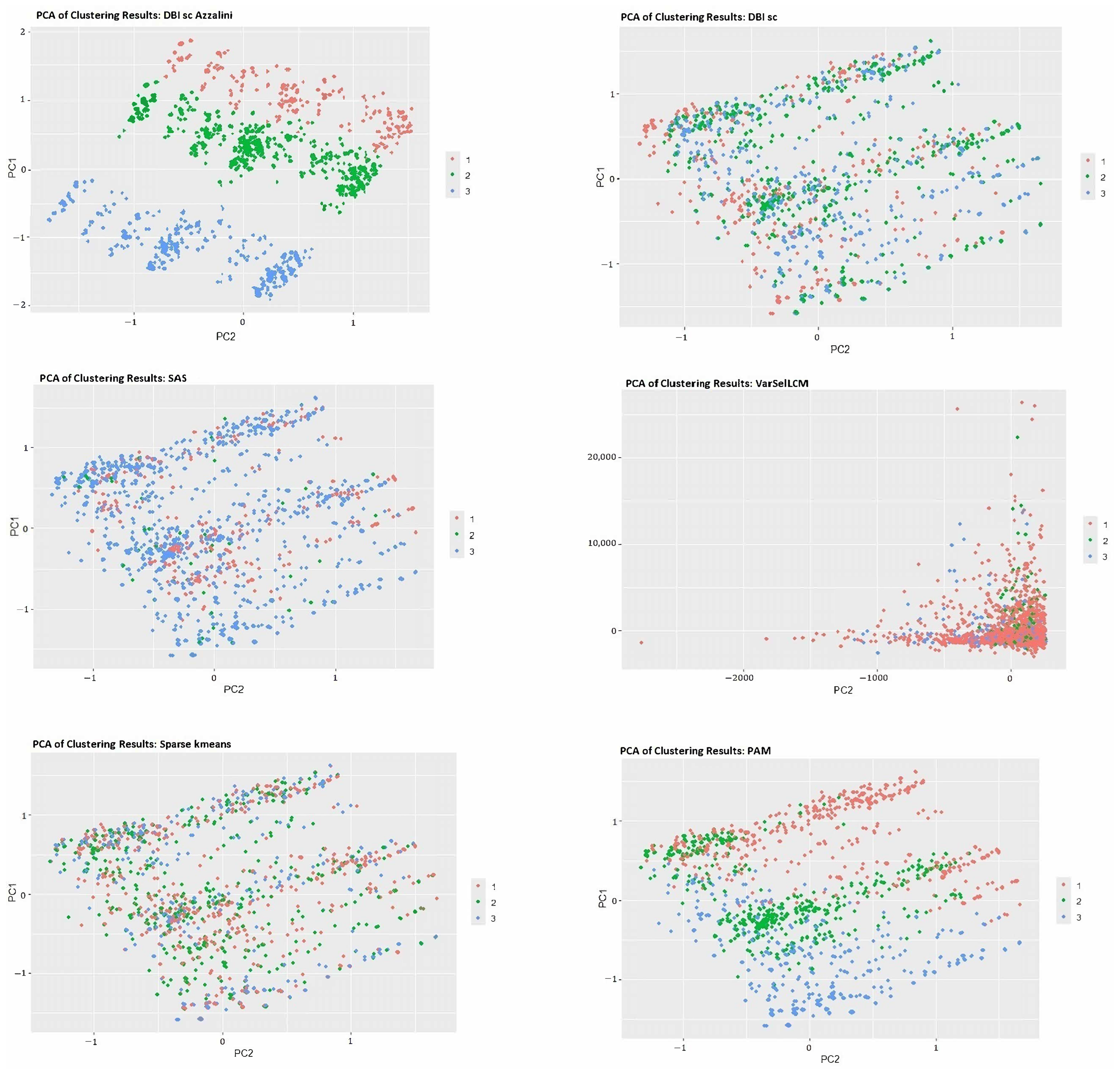
The clustering results reveal that level of education has a notable influence on cluster formation. Specifically, clients tend to group according to their education level, with distinct patterns emerging between individuals with primary, secondary, and tertiary education. This effect is clearly visible in the PCA visualization (Figure 4), where clusters partially align along the axis associated with the ordinal education variable. The DBI–SC–Azzalini method, which incorporates a score-based transformation for ordinal features, captures this structure effectively, demonstrating that preserving ordinal information enhances interpretability and improves the meaningfulness of the resulting clusters.

Figure 4 shows a PCA projection of the clustered data ($K=3$). The separation between education levels is visible along the primary principal component, confirming that ordinal information contributes to the discriminative power of the clustering. This further illustrates that DBI–SC–Azzalini is particularly suitable for datasets in which ordinal variables play a central role.

Overall, the real-data experiment confirms the main claims of this work: (i) quantile-based ordinal encoding improves clustering quality; (ii) the proposed mDBI criterion induces meaningful sparsity; (iii) DBI–SC–Azzalini offers superior interpretability and robust performance on mixed-type, high-dimensional datasets.

7. Conclusions

In this paper, we introduced DBI–SC–Azzalini, a new sparse clustering framework tailored for high-dimensional mixed-type data. The proposed method combines a unified dissimilarity index integrating continuous, ordinal, and nominal variables with adaptive feature weighting driven by the Davies–Bouldin criterion. A key component of our approach is the use of Azzalini’s [16] score-based transformation for ordinal variables, which provides a principled and model-based embedding that preserves the intrinsic ordering while remaining compatible with Euclidean-based clustering. This synergy allows the method to perform clustering and variable selection simultaneously within a coherent optimization framework.

Through extensive simulation studies, we demonstrated that DBI–SC–Azzalini consistently outperforms several state-of-the-art competitors, including Sparse k-means, VarSelLCM, and PAM based on Gower distance, in terms of both clustering accuracy and the reliability of variable selection. The proposed method shows particular robustness in the presence of noise variables and heterogeneous data structures. Furthermore, the application to a real-world bank marketing dataset highlighted the interpretability and practical relevance of the resulting clusters, along with a significant reduction in dimensionality.

Several directions for future research naturally arise from this work. First, improving computational scalability for ultra-high-dimensional settings constitutes an important perspective. Second, extending the framework to settings with missing values, longitudinal or hierarchical mixed-type data, or constraints on cluster shapes could broaden applicability. Finally, investigating theoretical guarantees under weaker assumptions and integrating deep or representation-learning techniques with the proposed dissimilarity measure represent promising avenues.

Overall, DBI–SC–Azzalini provides a flexible, interpretable, and theoretically grounded contribution to the analysis of mixed-type data, filling an important methodological gap and offering a solid foundation for future extensions in sparse clustering.