Estimation of the Inverse Power Lindley Distribution Parameters Using Ranked Set Sampling with an Application to Failure Time Data

Abstract

In this paper, the ranked set sampling method (RSS) is considered for estimating the inverse power Lindley distribution (IPLD) parameters and compared with the commonly simple random sampling. Different estimation methods are investigated including the commonly maximum likelihood, minimum distance estimation methods (Anderson Darling (AD), right tail Anderson Darling, left tail Anderson Darling, AD left tail second order, Cramér-von Mises), methods of maximum and minimum spacing distance (maximum product spacing distance, minimum spacing distance), methods of ordinary and weighted least squares, and the Kolmogorov–Smirnov method. A simulation study is conducted to compare these methods using RSS and SRS based on the same number of measured units in terms of mean squared error, bias, efficiency, and mean relative estimation error. A failure data set is fitted to the IPLD and the proposed estimation methods are applied to the data.

1. Introduction

Ranked set sampling (RSS) is an advanced statistical sampling technique introduced by [1] that improves parameter estimation accuracy compared to simple random sampling (SRS). It is particularly beneficial in situations where precise measurements are costly, time-consuming, or destructive, while ranking the units is relatively easy and inexpensive. The RSS is widely applied in various fields, including agriculture, environmental science, reliability analysis, and medical research. Over time, it has been adapted into different variations, such as modified RSS, extreme RSS, median RSS, and multistage RSS to suit specific research needs. Its efficiency and flexibility make RSS an essential tool in modern statistical inference and data collection methodologies.

Let X be a random variable representing a characteristic of interest with mean $\mu =E\left(X\right)$ and variance ${\sigma }^2$. Let $X_{ij}$ denote the j-th observation in the i-th set, where $i=1,2,\dots ,m$ and $j=1,2,\dots ,m$.

The RSS process can be performed with m sets, each of size m as in the following steps:

• Chose m random sets from the population of interest as

  $$\left\{\begin{array}{cccc}{X}_{11},& X_{12},& \dots & ,X_{1m}\\ X_{21},& X_{22},& \dots & ,X_{2m}\\ ⋮& ⋮& \ddots & ⋮\\ X_{m1},& X_{m2},& \dots & ,X_{mm}\end{array}\right\}$$
• Rank the units in each set through an inexpensive technique, for example, visual ranking or using an auxiliary variable as

  $$\left\{\begin{array}{cccc}{X}_{1\left(1\right)},& X_{1\left(2\right)},& \dots & ,X_{1\left(m\right)}\\ X_{2\left(1\right)}& X_{2\left(2\right)}& \dots & ,X_{2\left(m\right)}\\ ⋮& ⋮& \ddots & ⋮\\ X_{m\left(1\right)},& X_{m\left(2\right)},& \dots & ,X_{m\left(m\right)}\end{array}\right\}$$

  where $X_{i\left(j\right)}$ denotes the j-th smallest order unit in i-th set.
• From the i-th set, select the i-th ranked unit $X_{i\left(i\right)}$, by selecting from the first set, the smallest-ranked observation $X_{1\left(1\right)}$ is measured, from the second set, the second-smallest observation $X_{2\left(2\right)}$ is measured. This process continues, with the m-th set contributing the highest-ranked observation $X_{m\left(m\right)}$ as
  Then, the final RSS sample which can be used for actual measurement is: $X_{\mathrm{RSS}}=\{X_{1\left(1\right)},X_{2\left(2\right)},\dots ,X_{m\left(m\right)}\}.$

The probability density function (pdf) and cumulative distribution function (CDF) of the $X_{(i:m)}$, respectively, are given by

$$f\left(x_{(i:m)}\right)={\displaystyle \frac{m!}{(i-1)!(m-i)!}}f\left(x_{(i:m)}\right){\left[F\left(x_{(i:m)j}\right)\right]}^{i-1}{[1-F\left(x_{(i:m)}\right)]}^{m-i},$$

and

$$F\left(x_{(k:m)j}\right)=\sum _{h=k}^m{\displaystyle \frac{m!}{h!(m-h)!}}{\left[F\left(x_{(k:m)}\right)\right]}^h{[1-F(x_{(k:m)};)]}^{m-h}.$$

The final RSS sample consists of the measured values $X_{i\left(i\right)}$ for $i=1,2,\dots ,m$. The RSS-based estimator for the population mean is given by ${\widehat{\mu }}_{RSS}={\displaystyle \frac{1}{m}}{\sum }_{i=1}^m{X}_{i\left(i\right)},$ which is generally more efficient than the simple SRS estimator. It can be shown that $E\left({\widehat{\mu }}_{RSS}\right)=\mu$, that is the RSS estimator is unbiased for $\mu$ [2]. The variance of the RSS mean estimator is generally lower than that of the SRS estimator ($\mathrm{Var}\left({\widehat{\mu }}_{RSS}\right)\le \mathrm{Var}\left({\widehat{\mu }}_{SRS}\right)$) based on the same size of measured units with variance:

$${\widehat{\sigma }}_{RSS}^2={\displaystyle \frac{1}{m-1}}\sum _{i=1}^m{(X_{i\left(i\right)}-{\widehat{\mu }}_{RSS})}^2.$$

In general, the RSS enhances estimation accuracy by incorporating ranking information, particularly when ranking is highly correlated with actual measurements. The efficiency gain depends on the strength of ranking and the underlying population distribution. In many practical applications, RSS achieves the same estimation precision as SRS but with a smaller sample size, making it a valuable method in scenarios where exact measurements are costly or time-consuming.

Recently, numerous studies have explored RSS by introducing modifications or applying it to estimate population parameters across various fields.

Ref. [3] proposed balanced groups RSS for mean estimation. Ref. [4] suggested a multistage RSS for estimating the population mean, which increases efficiency for a fixed sample size. A modified robust extreme RSS is proposed by [5] for estimating the population mean. Ref. [6] offered a mixed RSS as a variation of the RSS for parameters estimation. Ref. [7] studied the maximum likelihood estimators using RSS of the log–logistic distribution parameters. Ref. [8] investigated the problem of estimating log–logistic parameters using the moving extremes RSS. Ref. [9] considered the RSS in estimating the inverted Kumaraswamy distribution parameters. Ref. [10] investigated the population mean under stratified RSS. Ref. [11] studied the RSS in estimating the Xgamma distribution parameters with an application to real data. Ref. [12] introduced a review of RSS and its modified methods in developing control charts. Ref. [13] proposed the dual RSS method. Ref. [14] investigated the RSS in various estimation methods for the power logarithmic distribution. Ref. [15] suggested new modification to the median quartile double RSS for estimating the population mean. Ref. [16] utilized the neutrosophic median RSS for mean estimation with an application to demographic data. Ref. [17] considered mean estimation using RSS in the presence of measurement errors. Ref. [18] recommended the RSS in evaluating the performance of control charts. Ref. [19] used the RSS in estimating the parameters of the unit Lindley distribution. Ref. [20] used the RSS for estimating the stress-strength reliability for the Beta-Lomax distribution. Ref. [21] investigated the RSS in estimating the parameter of the exponential-Poisson distribution. Ref. [22] considered the MRSS for estimating the log–logistic distribution using median RSS based on the maximum likelihood estimation.

The Lindley distribution is proposed by [23] by mixing the exponential and gamma distributions with respective pdfs:

$$f_1(x\mid \beta )=\beta e^{-\beta x},x>0,\beta >0,\mathrm{and}{f}_2(x\mid 2,\beta )={\beta }^{2}x{e}^{-\beta x},x>0,\beta >0$$

to get the pdf of Lindley distribution as

$$f(x\mid \beta )={\displaystyle \frac{{\beta }^2}{1+\beta }}(1+x)e^{-\beta x},x>0,\beta >0.$$

Due to the importance of this distribution, many modifications and applications for this distribution are investigated in the literature as the inverse Lindley distribution by [24], the power Lindley distribution by [25], which is a mixture of Weibull distribution with shape parameter $\alpha$ and scale parameter $\beta$ and the generalized gamma distribution with scale parameter $\beta$, and shape parameters 2 and $\alpha$. Ref. [26] considered Bayesian and non-Bayesian estimations of truncated inverse power Lindley distribution under progressively type-II censored data and studied it by Bayesian and non-Bayesian estimations. Ref. [27] suggested heavy-tailed inverse power Lindley Type-I model.

The pdf of the inverse power Lindley distribution [28] is given by

$$f(x\mid \alpha ,\beta )={\displaystyle \frac{\alpha {\beta }^2}{1+\beta }}\left({\displaystyle \frac{1+x^{\alpha }}{x^{2\alpha +1}}}\right)e^{-{\displaystyle \frac{\beta }{x^{\alpha }}}},x>0,\alpha >0,\beta >0,$$

(1)

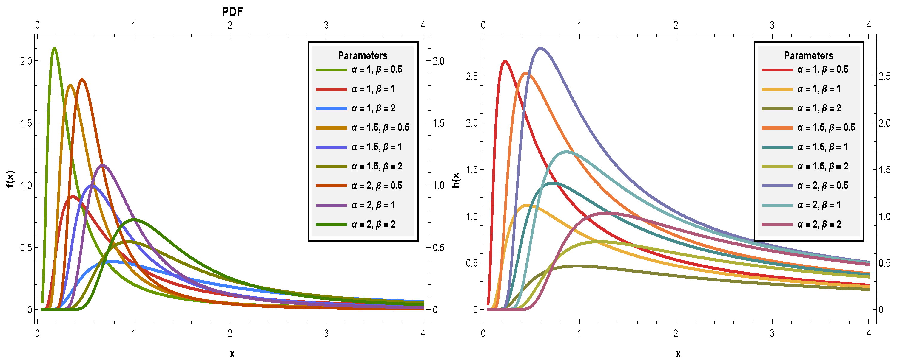
where $\alpha$ is the location parameter and $\beta$ the scale parameter. The corresponding cumulative distribution function (CDF) and hazard rate function (HRF) for the PILD are respectively in Figure 1, given by

$$F(x\mid \alpha ,\beta )=\left(1+{\displaystyle \frac{\beta }{1+\beta }}·{\displaystyle \frac{1}{x^{\alpha }}}\right)e^{-{\displaystyle \frac{\beta }{x^{\alpha }}}},x>0,\alpha >0,\beta >0$$

$$h(x\mid \alpha ,\beta )={\displaystyle \frac{\alpha {\beta }^2(1+x^{-\alpha })}{x\left[-\beta +x^{\alpha }(1+\beta )(e^{\frac{\beta }{x^{\alpha }}}-1)\right]}},x>0,\alpha >0,\beta >0.$$

Figure 1. The IPLD pdf and HRF plots.

The main objectives of the study are

• To estimate the parameters of the inverse power Lindley distribution using RSS technique, and to compare the performance of RSS with the SRS method in parameter estimation.
• To evaluate and compare multiple estimation techniques, including: maximum Likelihood estimation, minimum distance estimation methods (Anderson–Darling, right-tail AD, left-tail AD, left-tail second order AD, Cramér–von Mises), maximum and minimum spacing distance methods, ordinary and weighted least squares methods, and the Kolmogorov–Smirnov method.
• To conduct a simulation study assessing each estimation method under RSS and SRS using performance criteria such as mean squared error (MSE), bias, efficiency, and mean relative estimation error (MRE).
• To apply the proposed estimation approaches to a real failure data set to demonstrate the practical utility of RSS in estimating IPLD parameters.

The rest of this paper is organized as follows. In Section 2, different estimation methods are introduced. A detailed numerical simulations are given in Section 3. An application of real data is presented in Section 4. In Section 5, main results for the work are presented along with some directions for further works.

2. Methods of Estimation

In this section, we investigate fifteen estimation method to estimate the parameters $\alpha$ and $\beta$ of the I-PL distribution. Within this framework, we denote $t_{(s:v)h}$ as the $sth$ ranked observation (i.e., the $sth$ order statistic) in the $sth$ subset of the $hth$ cycle, where s ranges from 1 to d and h ranges from 1 to v. These observations form the RSS data for T, with a total sample size of $m=dv$. For simplification, we represent the selected sample under the RSS design as $t_{sh}.$

2.1. Maximum Likelihood Estimation

This section derives the maximum likelihood estimators (MLEs) for parameters $\alpha$ and $\beta$ of the I-PL distribution using the RSS methodology. MLEs is the most widely used estimation method in statistics due to its optimal asymptotic properties (consistency, asymptotic efficiency, and asymptotic normality). Let $z_{sh}=(z_{sh},s=1,\dots ,d,h=1,2,\dots ,v)$ represent the observed RSS data with sample size $m=dv$, where d indicates the set size and v denotes the number of cycles, all sampled from the I-PL distribution.

Based on this RSS data, the likelihood function $L(\alpha ,\beta )$ is expressed as

$$L(\alpha ,\beta )=\prod _{h=1}^v\prod _{s=1}^d{g}_{(s:d)}(t_{sh},\alpha ,\beta ),$$

(2)

where

$$\begin{array}{c}{g}_{(s:d)}(t_{sh},\alpha ,\beta )={\displaystyle \frac{1}{\mathrm{B}(s,d-s+1)}}{\left[G(t_{sh},\alpha ,\beta )\right]}^{s-1}{\left[1-G(t_{sh},\alpha ,\beta )\right]}^{d-s}g(t_{sh},\alpha ,\beta )\hfill \\ ={\displaystyle \frac{\alpha {\beta }^2}{(1+\beta )\mathrm{B}(s,d-s+1)}}{\left[\left({\displaystyle \frac{\beta }{\left(\beta +1\right)t_{sh}^{\alpha }}}+1\right){\mathrm{e}}^{-{\displaystyle \frac{\beta }{t_{sh}^{\alpha }}}}\right]}^{s-1}\hfill \\ \times \left({\displaystyle \frac{1+t_{sh}^{\alpha }}{t_{sh}^{2\alpha +1}}}\right){\mathrm{e}}^{-{\displaystyle \frac{\beta }{t_{sh}^{\alpha }}}}{\left[1-\left({\displaystyle \frac{\beta }{\left(\beta +1\right)t_{sh}^{\alpha }}}+1\right){\mathrm{e}}^{-{\displaystyle \frac{\beta }{t_{sh}^{\alpha }}}}\right]}^{d-s}.\hfill \end{array}$$

The log-likelihood function of (2) is as follows:

$$\begin{array}{c}logL\propto mlog\left(\alpha \right)+2mlog\left(\beta \right)-mlog(\beta +1)+{\displaystyle \sum _{h=1}^v\sum _{s=1}^d(s-1)log}\left(\mathsf{\Psi }(t_{sh},\alpha ,\beta )\right)-\beta {\displaystyle \sum _{h=1}^v\sum _{s=1}^d{\displaystyle \frac{s}{t_{sh}^{\alpha }}}}\hfill \\ +{\displaystyle \sum _{h=1}^v\sum _{s=1}^d(d-s)log\left(1-\mathsf{\Psi }(t_{sh},\alpha ,\beta ){\mathrm{e}}^{-{\displaystyle \frac{\beta }{t_{sh}^{\alpha }}}}\right)}+{\displaystyle \sum _{h=1}^v\sum _{s=1}^{d}log}\left({\displaystyle \frac{1+t_{sh}^{\alpha }}{t_{sh}^{2\alpha +1}}}\right),\hfill \end{array}$$

where $\mathsf{\Psi }(t_{sh},\alpha ,\beta )={\displaystyle \frac{\beta }{\left(\beta +1\right)t_{sh}^{\alpha }}}+1.$

The MLEs ${\tilde{\alpha }}_1$ of $\alpha$, and ${\tilde{\beta }}_1$ of $\beta$ can be obtained by solving simultaneously the following normal equations:

$$\begin{array}{c}{\displaystyle \frac{\partial logl}{\partial \alpha }}={\displaystyle \frac{m}{\alpha }}+{\displaystyle \sum _{h=1}^v\sum _{s=1}^d}{\displaystyle \frac{(s-1){\mathsf{\Psi }}_{\alpha }^{\prime }(t_{sh},\alpha ,\beta )}{\mathsf{\Psi }(t_{sh},\alpha ,\beta )}}+\beta {\displaystyle \sum _{h=1}^v\sum _{s=1}^d{\displaystyle \frac{slog\left(t\right)}{t_{sh}^{\alpha }}}}-{\displaystyle \sum _{h=1}^v\sum _{s=1}^d}{t}_{sh}^{-2\alpha -1}log\left(t_{sh}\right)\left(t_{sh}^{\alpha }+2\right)\hfill \\ -{\displaystyle \sum _{h=1}^v\sum _{s=1}^d}{\displaystyle \frac{(d-s){\mathsf{\Psi }}_{\alpha }^{\prime }(t_{sh},\alpha ,\beta ){\mathrm{e}}^{-\frac{\beta }{t_{sh}^{\alpha }}}+\mathsf{\Psi }(t_{sh},\alpha ,\beta )log\left(t_{sh}\right)\beta {\mathrm{e}}^{-\frac{\beta }{t_{sh}^{\alpha }}}{t}_{sh}^{-\alpha }}{1-\mathsf{\Psi }(t_{sh},\alpha ,\beta ){\mathrm{e}}^{-\frac{\beta }{t_{sh}^{\alpha }}}}}=0\hfill \end{array}$$

and

$$\begin{array}{c}{\displaystyle \frac{\partial logl}{\partial \beta }}={\displaystyle \frac{2m}{\beta }}+{\displaystyle \sum _{h=1}^v\sum _{s=1}^d}{\displaystyle \frac{(s-1){\mathsf{\Psi }}_{\beta }^{\prime }(t_{sh},\alpha ,\beta )}{\mathsf{\Psi }(t_{sh},\alpha ,\beta )}}-{\displaystyle \sum _{h=1}^v\sum _{s=1}^d{\displaystyle \frac{s}{t_{sh}^{\alpha }}}}\hfill \\ -{\displaystyle \sum _{h=1}^v\sum _{s=1}^d}{\displaystyle \frac{(d-s){\mathsf{\Psi }}_{\beta }^{\prime }(t_{sh},\alpha ,\beta ){\mathrm{e}}^{-\frac{\beta }{t_{sh}^{\alpha }}}-\mathsf{\Psi }(t_{sh},\alpha ,\beta )t^{-\alpha }{\mathrm{e}}^{-\frac{\beta }{t_{sh}^{\alpha }}}}{1-\mathsf{\Psi }(t_{sh},\alpha ,\beta ){\mathrm{e}}^{-\frac{\beta }{t_{sh}^{\alpha }}}}}=0,\hfill \end{array}$$

where, ${\mathsf{\Psi }}_{\alpha }^{\prime }(t_{sh},\alpha ,\beta )=-{\displaystyle \frac{log\left(t_{sh}\right)\beta }{t_{sh}^{\alpha }\left(\beta +1\right)}}$ and ${\mathsf{\Psi }}_{\beta }^{\prime }(t_{sh},\alpha ,\beta )={\displaystyle \frac{1}{t_{sh}^{\alpha }{\left(\beta +1\right)}^2}}$.

To solve for ${\tilde{\alpha }}_{MLE}$ and ${\tilde{\beta }}_{MLE}$, numerical methods are required since these estimators cannot be expressed in closed form. Nonlinear optimization algorithms such as the Newton–Raphson iterative method would be appropriate for computing these values.

2.2. Minimum Distance Estimation Methods

Estimation methods that rely on minimizing well-established goodness-of-fit statistics are often effective and yield reliable results in various scenarios. In this study, five widely used techniques are considered, each aiming to minimize the discrepancy between the theoretical and empirical cumulative distribution functions.

2.2.1. Anderson–Darling

The Anderson–Darling method is particularly appropriate for capturing tail behavior accurately. Consider an ordered sample $t_{(1:m)},t_{(2:m)},\dots ,t_{(m:m)}$ obtained from a RSS of size $m=dv$, where d represents the set size and v is the cycle number, drawn from the I-PL distribution. The Anderson–Darling estimates (ADEs) for $\alpha$ and $\beta$, denoted as ${\tilde{\alpha }}_{AD}$ and ${\tilde{\beta }}_{AD}$, are obtained by minimizing the following function:

$${\vartheta }_1(\alpha ,\beta )=-m-{\displaystyle \frac{1}{m}}\sum _{i=1}^m(2i-1)\left[logG\left(t_{(i_1:n)}\mid \alpha ,\beta \right)+logS\left(t_{(1+m-i:m)}\mid \alpha ,\beta \right)\right],$$

(3)

where $S\left(.\left|\alpha ,\beta \right.\right)$ represents the survival function. Instead of directly using (3), the values ${\tilde{\alpha }}_{ADE}$ and ${\tilde{\beta }}_{ADE}$ can be numerically determined by solving the following nonlinear equations:

$${\displaystyle \frac{\partial {\vartheta }_1(\alpha ,\beta )}{\partial \alpha }}=\sum {i=1}^m(2i-1)\left[{\displaystyle \frac{\delta \alpha \left(t(i:m)\left|\alpha ,\beta \right.\right)}{G\left(t_{(i:m)}\left|\alpha ,\beta \right.\right)}}+{\displaystyle \frac{\delta \alpha \left(t(1+m-i:m)\left|\alpha ,\beta \right.\right)}{S\left(t_{(1+m-i:m)}\left|\alpha ,\beta \right.\right)}}\right]=0,$$

and

$${\displaystyle \frac{\partial {\vartheta }_1(\alpha ,\beta )}{\partial \beta }}=\sum {i=1}^m(2i-1)\left[{\displaystyle \frac{\delta \beta \left(t(i:m)\left|\alpha ,\beta \right.\right)}{G\left(t_{(i:m)}\left|\alpha ,\beta \right.\right)}}+{\displaystyle \frac{\delta \beta \left(t(1+m-i:m)\left|\alpha ,\beta \right.\right)}{S\left(t_{(1+m-i:m)}\left|\alpha ,\beta \right.\right)}}\right]=0,$$

where

$${\delta }_{\alpha }\left(t_{(i:m)}\left|\alpha ,\beta \right.\right)={\displaystyle \frac{\partial }{\partial \alpha }}G\left(z_{(i_1:n)}\left|\alpha ,\beta \right.\right)={\displaystyle \frac{log\left(t_{(i:m)}\right)\left({t_{(i:m)}}^{\alpha }+1\right){\beta }^2{\mathrm{e}}^{-\frac{\beta }{{t_{(i:m)}}^{\alpha }}}}{{t_{(i:m)}}^{2\alpha }\left(\beta +1\right)}},$$

(4)

and

$${\delta }_{\beta }\left(t_{(i:m)}\left|\alpha ,\beta \right.\right)={\displaystyle \frac{\partial }{\partial \beta }}G\left(z_{(i_1:n)}\left|\alpha ,\beta \right.\right)=-{\displaystyle \frac{\beta \left(\left({t_{(i:m)}}^{\alpha }+1\right)\beta +2{t_{(i:m)}}^{\alpha }+1\right){\mathrm{e}}^{-\frac{\beta }{{t_{(i:m)}}^{\alpha }}}}{{t_{(i:m)}}^{2\alpha }{\left(\beta +1\right)}^2}},$$

(5)

and $\delta \alpha \left(t(i-1:m)\left|\alpha ,\beta \right.\right)$ and $\delta \beta \left(t(i-1:m)\left|\alpha ,\beta \right.\right)$ have similar expressions with the ordered sample $t_{(i-1:m)}$.

2.2.2. Right-Tail Anderson–Darling

The Right-Tail Anderson–Darling specifically emphasizes the right tail of the distribution. Consider an ordered sample $t_{(1:m)},t_{(2:m)},\dots ,t_{(m:m)}$ obtained from an RSS of size $m=dv$, where d represents the set size and v is the cycle number, drawn from the I-PL distribution. The right-tail Anderson–Darling estimates (RTADEs) for $\alpha$ and $\beta$, denoted as ${\tilde{\alpha }}_{RTADE}$ and ${\tilde{\beta }}_{RTADE}$, are obtained by minimizing the following function:

$${\vartheta }_2(\alpha ,\beta )={\displaystyle \frac{m}{2}}-2\sum {i=1}^{m}G\left(t_{(i:m)}\left|\alpha ,\beta \right.\right)-{\displaystyle \frac{1}{m}}\sum _{i=1}^m(2i-1)logS\left(t_{(m+1-i:m)}\left|\alpha ,\beta \right.\right).$$

(6)

Instead of directly using (6), the values ${\tilde{\alpha }}_{RTADE}$ and ${\tilde{\beta }}_{RTADE}$ can be determined numerically by solving the following nonlinear equations:

$${\displaystyle \frac{\partial {\vartheta }_2(\alpha ,\beta )}{\partial \alpha }}=-2\sum _{i=1}^m{\displaystyle \frac{{\delta }_{\alpha }\left(t_{(i:m)}\left|\alpha ,\beta \right.\right)}{G\left(t_{(i:m)}\left|\alpha ,\beta \right.\right)}}-{\displaystyle \frac{1}{m}}\sum _{i=1}^m(2i-1)\left[{\displaystyle \frac{{\delta }_{\alpha }\left(t_{(1+m-i:m)}\left|\alpha ,\beta \right.\right)}{S\left(t_{(1+m-i:m)}\left|\alpha ,\beta \right.\right)}}\right]=0,$$

and

$${\displaystyle \frac{\partial {\vartheta }_2(\alpha ,\beta )}{\partial \beta }}=-2\sum _{i=1}^m{\displaystyle \frac{{\delta }_{\beta }\left(t_{(i:m)}\left|\alpha ,\beta \right.\right)}{G\left(t_{(i:m)}\left|\alpha ,\beta \right.\right)}}-{\displaystyle \frac{1}{m}}\sum _{i=1}^m(2i-1)\left[{\displaystyle \frac{{\delta }_{\beta }\left(t_{(1+m-i:m)}\left|\alpha ,\beta \right.\right)}{S\left(t_{(1+m-i:m)}\left|\alpha ,\beta \right.\right)}}\right]=0,$$

where ${\delta }_{\alpha }\left(.\left|\alpha ,\beta \right.\right)$ and ${\delta }_{\beta }\left(.\left|\alpha ,\beta \right.\right)$ are given in (4) and (5).

2.2.3. Left-Tail Anderson–Darling

The Left-Tail Anderson–Darling focuses on the left tail of the distribution. It is useful when early failures or small values are of particular concern, such as in quality control applications. Let $t_{(1:m)},t_{(2:m)},\dots ,t_{(m:m)}$ be an ordered sample obtained from the I-PL distribution and forming an RSS of size $m=sw$, where s represents the set size and w is the cycle number. The Left-Tail Anderson–Darling estimates (LTADEs) for $\alpha$ and $\beta$, denoted as ${\tilde{\alpha }}_{LTADE}$ and ${\tilde{\beta }}_{LTADE}$, are determined by minimizing the following function:

$${\vartheta }_3(\alpha ,\beta )={\displaystyle \frac{-3m}{2}}+2\sum _{i=1}^{m}G\left(t_{(i:m)}\left|\alpha ,\beta \right.\right)-{\displaystyle \frac{1}{m}}\sum _{i=1}^m(2i-1)logG\left(t_{(i:m)}\left|\alpha ,\beta \right.\right).$$

(7)

The following nonlinear equations can be solved numerically instead of (7) to obtain ${\tilde{\alpha }}_{LTADE}$ and ${\tilde{\beta }}_{LTADE}$:

$${\displaystyle \frac{\partial {\vartheta }_3(\alpha ,\beta )}{\partial \alpha }}=2\sum _{i=1}^m{\delta }_{\alpha }\left(t_{(i:m)}\left|\alpha ,\beta \right.\right)-{\displaystyle \frac{1}{m}}\sum _{i=1}^m{\displaystyle \frac{(2i-1){\delta }_{\alpha }\left(t_{(i:m)}\left|\alpha ,\beta \right.\right)}{G\left(t_{(i:m)}\left|\alpha ,\beta \right.\right)}}=0,$$

and

$${\displaystyle \frac{\partial {\vartheta }_3(\alpha ,\beta )}{\partial \beta }}=2\sum _{i=1}^m{\delta }_{\beta }\left(t_{(i:m)}\left|\alpha ,\beta \right.\right)-{\displaystyle \frac{1}{m}}\sum _{i=1}^m{\displaystyle \frac{(2i-1){\delta }_{\beta }\left(t_{(i:m)}\left|\alpha ,\beta \right.\right)}{G\left(t_{(i:m)}\left|\alpha ,\beta \right.\right)}}=0,$$

where ${\delta }_{\alpha }\left(.\left|\alpha ,\beta \right.\right)$ and ${\delta }_{\beta }\left(.\left|\alpha ,\beta \right.\right)$ are given in (4) and (5).

2.2.4. AD Left-Tail Second Order

The Left-Tail Anderson–Darling second-order provides enhanced emphasis on the extreme left-tail with second-order weighting and offers even more sensitivity to the behavior of the distribution near zero, which can be critical for certain applications. Let $t_{(1:m)},t_{(2:m)},\dots ,t_{(m:m)}$ be an ordered sample constructed using the I-PL distribution, resulting in an RSS of size $m=sw$ with set size s and cycle number w. The Left-Tail Anderson–Darling second-order estimate (ADSOE) for $\alpha$ and $\beta$, denoted as ${\tilde{\alpha }}_5$ and ${\tilde{\beta }}_5$, is obtained by minimizing the function below:

$${\vartheta }_4(\alpha ,\beta )=2\sum _{i=1}^{m}log\left[G\left(t_{(i:m)}\left|\alpha ,\beta \right.\right)\right]+{\displaystyle \frac{1}{m}}\sum _{i=1}^m{\displaystyle \frac{(2i-1)}{G\left(t_{(i:m)}\left|\alpha ,\beta \right.\right)}}.$$

(8)

Instead of solving Equation (8) directly, one can solve the following nonlinear equations to obtain ${\tilde{\alpha }}_{ADSOE}$ and ${\tilde{\beta }}_{ADSOE}$:

$${\displaystyle \frac{\partial {\vartheta }_4(\alpha ,\beta )}{\partial \alpha }}=2\sum _{i=1}^m{\displaystyle \frac{{\delta }_{\alpha }\left(t_{(i:m)}\left|\alpha ,\beta \right.\right)}{G\left(t_{(i:m)}\left|\alpha ,\beta \right.\right)}}-{\displaystyle \frac{1}{m}}\sum _{i=1}^m{\displaystyle \frac{(2i-1){\delta }_{\alpha }\left(t_{(i:m)}\left|\alpha ,\beta \right.\right)}{G^2\left(t_{(i:m)}\left|\alpha ,\beta \right.\right)}}=0,$$

and

$${\displaystyle \frac{\partial {\vartheta }_4(\alpha ,\beta )}{\partial \beta }}=2\sum _{i=1}^m{\displaystyle \frac{{\delta }_{\beta }\left(t_{(i:m)}\left|\alpha ,\beta \right.\right)}{G\left(t_{(i:m)}\left|\alpha ,\beta \right.\right)}}-{\displaystyle \frac{1}{m}}\sum _{i=1}^m{\displaystyle \frac{(2i-1){\delta }_{\beta }\left(t_{(i:m)}\left|\alpha ,\beta \right.\right)}{G^2\left(t_{(i:m)}\left|\alpha ,\beta \right.\right)}}=0,$$

where ${\delta }_{\alpha }\left(.\left|\alpha ,\beta \right.\right)$ and ${\delta }_{\beta }\left(.\left|\alpha ,\beta \right.\right)$ are given in (4) and (5).

2.2.5. Cramér–von Mises Estimators

The Cramér–von Mises provides balanced estimation across the entire support of the distribution without emphasizing any particular region, making it a robust general-purpose estimator. Let $t_{(1:m)},t_{(2:m)},\dots ,t_{(m:m)}$ be an ordered sample created using the I-PL distribution, which yields an RSS of size $m=dv$, where d is the set size and v is the cycle number. The Cramér–von Mises estimates (CVMEs) for $\alpha$ and $\beta$, denoted as ${\tilde{\alpha }}_{CVME}$ and ${\tilde{\beta }}_{CVME}$, can be obtained by minimizing the following function:

$${\vartheta }_5(\alpha ,\beta )={\displaystyle \frac{1}{12m}}+\sum _{i=1}^m{\left\{G\left(v_{(i:m)}\left|\alpha ,\beta \right.\right)-{\displaystyle \frac{2i-1}{2m}}\right\}}^2.$$

(9)

Instead of using (9), one may solve the following nonlinear equations to obtain ${\tilde{\alpha }}_{CVME}$ and ${\tilde{\beta }}_{CVME}$:

$${\displaystyle \frac{\partial {\vartheta }_5(\alpha ,\beta )}{\partial \alpha }}=\sum _{i=1}^m\left\{G\left(t_{(i:m)}\left|\alpha ,\beta \right.\right)-{\displaystyle \frac{2i-1}{2m}}\right\}{\delta }_{\alpha }\left(t_{(i:m)}\left|\alpha ,\beta \right.\right)=0,$$

and

$${\displaystyle \frac{\partial {\vartheta }_5(\alpha ,\beta )}{\partial \beta }}=\sum _{i=1}^m\left\{G\left(t_{(i:m)}\left|\alpha ,\beta \right.\right)-{\displaystyle \frac{2i-1}{2m}}\right\}{\delta }_{\beta }\left(t_{(i:m)}\left|\alpha ,\beta \right.\right)=0,$$

where, ${\delta }_{\alpha }\left(.\left|\alpha ,\beta \right.\right)$ amd ${\delta }_{\beta }\left(.\left|\alpha ,\beta \right.\right)$ are given in (4) and (5).

2.3. Method of Maximum and Minimum Spacing Distance

The MPS approach was first presented by Cheng and Amin [29,30]. This approach depends on maximizing the geometric mean of the data’s spacings. For the most part, the MPS method is particularly effective for small samples and distributions with complex functional forms. MPS is less sensitive to outliers and model misspecification than MLE.

2.3.1. Maximum Product Spacing Distance

Suppose that $t_{(1:m)},t_{(2:m)},\dots ,t_{(m:m)}$ form an ordered sample creating an RSS of size $m=dv$, gathered from the I-PL distribution. The uniform spacing is then determined by

$${\mathsf{\Lambda }}_i=G\left(t_{(i:m)}\left|\alpha ,\beta \right.\right)-G\left(t_{(i-1:m)}\left|\alpha ,\beta \right.\right),i=1,2,\dots ,m+1.$$

Note that $G\left(t_{(0:m)}\alpha ,\beta \right)=0,G\left(t_{(m+1:m)}\left|\alpha ,\beta \right.\right)=1,$ and ${\displaystyle \sum _{i=1}^{m+1}}{\mathsf{\Lambda }}_i=1.$

The following function is maximized with respect to $\alpha$ and $\beta$ to obtain the MPS estimates (MPSEs) ${\tilde{\alpha }}_{MPSE}$ and ${\tilde{\beta }}_{MPSE}$:

$$\eta ={\displaystyle \frac{1}{m+1}}\sum _{i=1}^{m+1}log\left[{\mathsf{\Lambda }}_i\right].$$

The MPSEs ${\tilde{\alpha }}_{MPSE}$ and ${\tilde{\beta }}_{MPSR}$ can be obtained through the numerical computation of the following equations:

$${\displaystyle \frac{\partial \eta }{\partial \alpha }}={\displaystyle \frac{1}{m+1}}\sum _{i=1}^{m+1}{\displaystyle \frac{1}{{\mathsf{\Lambda }}_i}}\left[{\delta }_{\alpha }\left(t_{(i:m)}\left|\alpha ,\beta \right.\right)-{\delta }_{\alpha }\left(t_{(i-1:m)}\left|\alpha ,\beta \right.\right)\right]=0,$$

and

$${\displaystyle \frac{\partial \eta }{\partial \beta }}={\displaystyle \frac{1}{m+1}}\sum _{i=1}^{m+1}{\displaystyle \frac{1}{{\mathsf{\Lambda }}_i}}\left[{\delta }_{\beta }\left(t_{(i:m)}\left|\alpha ,\beta \right.\right)-{\delta }_{\beta }\left(t_{(i-1:m)}\left|\alpha ,\beta \right.\right)\right]=0,$$

where ${\delta }_{\alpha }\left(.\left|\alpha ,\beta \right.\right)$ and ${\delta }_{\beta }\left(.\left|\alpha ,\beta \right.\right)$ are given in (4) and (5).

2.3.2. Minimum Spacing Distance

Minimum spacing distance estimators provide a distribution-free approach that does not require complete specification of the likelihood function and is computationally simpler in some cases. Consider $t_{(1:m)},t_{(2:m)},\dots ,t_{(m:m)}$ as an ordered sample obtained from the I-PL distribution distribution, with cycle number w and set size s, forming an RSS of size $m=sw$. We can derive various parameter estimates by minimizing specific objective functions.

• Minimum spacing absolute distance
  By minimizing the following function, we obtain the minimum spacing absolute distance Estimates (MSADEs) ${\tilde{\alpha }}_{MSADE}$ of $\alpha$ and ${\tilde{\beta }}_{MSADE}$ of $\beta$:

  $${\chi }_1=\sum _{i=1}^{m+1}\left|{\mathsf{\Lambda }}_i-{\displaystyle \frac{1}{m+1}}\right|.$$

  (10)
  Instead of directly solving Equation (10), the following non-linear equations can be solved to obtain ${\tilde{\alpha }}_8$ and ${\tilde{\beta }}_8$:

  $${\displaystyle \frac{\partial {\chi }_1}{\partial \alpha }}=\sum _{i=1}^{m+1}{\displaystyle \frac{\left|{\mathsf{\Lambda }}_i-\frac{1}{m+1}\right|}{{\mathsf{\Lambda }}_i-\frac{1}{m+1}}}\left[{\delta }_{\alpha }\left(t_{(i:m)}\left|\alpha ,\beta \right.\right)-{\delta }_{\alpha }\left(t_{(i-1:m)}\left|\alpha ,\beta \right.\right)\right]=0,$$

  and

  $${\displaystyle \frac{\partial {\chi }_1}{\partial \beta }}=\sum _{i=1}^{m+1}{\displaystyle \frac{\left|{\mathsf{\Lambda }}_i-\frac{1}{m+1}\right|}{{\mathsf{\Lambda }}_i-\frac{1}{m+1}}}\left[{\delta }_{\beta }\left(t_{(i:m)}\left|\alpha ,\beta \right.\right)-{\delta }_{\beta }\left(t_{(i-1:m)}\left|\alpha ,\beta \right.\right)\right]=0,$$

  where ${\delta }_{\alpha }\left(.\left|\alpha ,\beta \right.\right)$ and ${\delta }_{\beta }\left(.\left|\alpha ,\beta \right.\right)$ are given in Equations (4) and (5).
• Minimum spacing absolute-log distance
  By minimizing the following function, we obtain and the minimum spacing absolute-log distance Estimates (MSALDEs) ${\tilde{\alpha }}_{MSALDE}$ of $\alpha$ and ${\tilde{\beta }}_{MSALDE}$ of $\beta$,

  $${\chi }_2=\sum _{i=1}^{m+1}\left|log\left({\mathsf{\Lambda }}_i\right)-log\left({\displaystyle \frac{1}{m+1}}\right)\right|$$

  (11)
  Similarly, we can solve the following non-linear equations instead of Equation (11) to obtain ${\tilde{\alpha }}_{MSALDE}$ and ${\tilde{\beta }}_{MSALDE}$:

  $${\displaystyle \frac{\partial {\chi }_2}{\partial \alpha }}=\sum _{i=1}^{m+1}{\displaystyle \frac{\left|log\left({\mathsf{\Lambda }}_i\right)-log\left(\frac{1}{m+1}\right)\right|}{\left(log\left({\mathsf{\Lambda }}_i\right)-log\left(\frac{1}{m+1}\right)\right)}}{\displaystyle \frac{1}{{\mathsf{\Lambda }}_i}}\left[{\delta }_{\alpha }\left(t_{(i:m)}\left|\alpha ,\beta \right.\right)-{\delta }_{\alpha }\left(t_{(i-1:m)}\left|\alpha ,\beta \right.\right)\right]=0,$$

  and

  $${\displaystyle \frac{\partial {\chi }_2}{\partial \beta }}=\sum _{i=1}^{m+1}{\displaystyle \frac{\left|log\left({\mathsf{\Lambda }}_i\right)-log\left(\frac{1}{m+1}\right)\right|}{\left(log\left({\mathsf{\Lambda }}_i\right)-log\left(\frac{1}{m+1}\right)\right)}}{\displaystyle \frac{1}{{\mathsf{\Lambda }}_i}}\left[{\delta }_{\beta }\left(t_{(i:m)}\left|\alpha ,\beta \right.\right)-{\delta }_{\beta }\left(t_{(i-1:m)}\left|\alpha ,\beta \right.\right)\right]=0,$$

  where ${\delta }_{\alpha }\left(.\left|\alpha ,\beta \right.\right)$ and ${\delta }_{\beta }\left(.\left|\alpha ,\beta \right.\right)$ are given in Equations (4) and (5).
• Minimum spacing square distance
  Next, by minimizing the following function, we determine the minimum spacing square distance Estimates (MSSDEs) ${\tilde{\alpha }}_{MSSDE}$ of $\alpha$ and ${\tilde{\beta }}_{MSSDE}$ of $\beta$:

  $$\left.\begin{array}{c}{\chi }_3={\displaystyle \sum _{i=1}^{m+1}}{\left({\mathsf{\Lambda }}_i-{\displaystyle \frac{1}{m+1}}\right)}^2,\end{array}\right].$$

  (12)
  Instead of solving Equation (12) directly, the following non-linear equations can be solved to obtain ${\tilde{\alpha }}_{10}$ and ${\tilde{\beta }}_{10}$:

  $${\displaystyle \frac{\partial {\chi }_3}{\partial \alpha }}=\sum _{i=1}^{m+1}\left({\mathsf{\Lambda }}_i-{\displaystyle \frac{1}{m+1}}\right)\left[{\delta }_{\alpha }\left(t_{(i:m)}\left|\alpha ,\beta \right.\right)-{\delta }_{\alpha }\left(t_{(i-1:m)}\left|\alpha ,\beta \right.\right)\right]=0,$$

  and

  $${\displaystyle \frac{\partial {\chi }_3}{\partial \beta }}=\sum _{i=1}^{m+1}\left({\mathsf{\Lambda }}_i-{\displaystyle \frac{1}{m+1}}\right)\left[{\delta }_{\beta }\left(t_{(i:m)}\left|\alpha ,\beta \right.\right)-{\delta }_{\beta }\left(t_{(i-1:m)}\left|\alpha ,\beta \right.\right)\right]=0,$$

  where ${\delta }_{\alpha }\left(.\left|\alpha ,\beta \right.\right)$ and ${\delta }_{\beta }\left(.\left|\alpha ,\beta \right.\right)$ are given in Equations (4) and (5).
• Minimum spacing square log-distance
  By minimizing the following function, we determine the minimum spacing square log-distance Estimates (MSSLDEs) ${\tilde{\alpha }}_{MSSLDE}$ of $\alpha$ and ${\tilde{\beta }}_{MSSLDE}$ of $\beta$,

  $${\chi }_4=\sum _{i=1}^{m+1}{\left(log\left({\mathsf{\Lambda }}_i\right)-log\left({\displaystyle \frac{1}{m+1}}\right)\right)}^2.$$

  (13)
  Similarly, we can solve the following non-linear equations instead of Equation (13) to obtain ${\tilde{\alpha }}_{MSSLDE}$ and ${\tilde{\beta }}_{MSSLDE}$:

  $${\displaystyle \frac{\partial {\chi }_4}{\partial \alpha }}=\sum _{i=1}^{m+1}\left(log\left({\mathsf{\Lambda }}_i\right)-log\left({\displaystyle \frac{1}{m+1}}\right)\right){\displaystyle \frac{1}{{\mathsf{\Lambda }}_i}}\left[{\delta }_{\alpha }\left(t_{(i:m)}\left|\alpha ,\beta \right.\right)-{\delta }_{\alpha }\left(t_{(i-1:m)}\left|\alpha ,\beta \right.\right)\right]=0,$$

  and

  $${\displaystyle \frac{\partial {\chi }_4}{\partial \beta }}=\sum _{i=1}^{m+1}\left(log\left({\mathsf{\Lambda }}_i\right)-log\left({\displaystyle \frac{1}{m+1}}\right)\right){\displaystyle \frac{1}{{\mathsf{\Lambda }}_i}}\left[{\delta }_{\beta }\left(t_{(i:m)}\left|\alpha ,\beta \right.\right)-{\delta }_{\beta }\left(t_{(i-1:m)}\left|\alpha ,\beta \right.\right)\right]=0,$$

  where ${\delta }_{\alpha }\left(.\left|\alpha ,\beta \right.\right)$ and ${\delta }_{\beta }\left(.\left|\alpha ,\beta \right.\right)$ are given in Equations (4) and (5).
• Minimum spacing Linex distance
  Finally, we can obtain the minimum spacing Linex distance Estimates (MSLDE) ${\tilde{\alpha }}_{MSLDE}$ of $\alpha$ and ${\tilde{\beta }}_{MSLDE}$ of $\beta$ by minimizing the following function:

  $${\chi }_5=\sum _{i=1}^{m+1}\left(e^{{\mathsf{\Lambda }}_i-{\displaystyle \frac{1}{m+1}}}-\left({\mathsf{\Lambda }}_i-{\displaystyle \frac{1}{m+1}}\right)-1\right).$$

  (14)
  Instead of solving Equation (14) directly, the following non-linear equations can be solved to obtain ${\tilde{\alpha }}_{MSLDE}$ and ${\tilde{\beta }}_{MSLDE}$:

  $${\displaystyle \frac{\partial {\chi }_5}{\partial \alpha }}=\sum _{i=1}^{m+1}(e^{{\mathsf{\Lambda }}_i-{\displaystyle \frac{1}{m+1}}}-1)\left[{\delta }_{\alpha }\left(t_{(i:m)}\left|\alpha ,\beta \right.\right)-{\delta }_{\alpha }\left(t_{(i-1:m)}\left|\alpha ,\beta \right.\right)\right]=0,$$

  and

  $${\displaystyle \frac{\partial {\chi }_5}{\partial \beta }}=\sum _{i=1}^{m+1}(e^{{\mathsf{\Lambda }}_i-{\displaystyle \frac{1}{m+1}}}-1)\left[{\delta }_{\beta }\left(t_{(i:m)}\left|\alpha ,\beta \right.\right)-{\delta }_{\beta }\left(t_{(i-1:m)}\left|\alpha ,\beta \right.\right)\right]=0,$$

  where ${\delta }_{\alpha }\left(.\left|\alpha ,\beta \right.\right)$ and ${\delta }_{\beta }\left(.\left|\alpha ,\beta \right.\right)$ are given in Equations (4) and (5).

2.4. Methods of Ordinary and Weighted Least Squares

The OLS estimates (OLSE) and WLS estimates (WLSE) were introduced by [31] to estimate the parameters of the beta distribution. They are simple to implement, computationally efficient, and provides reasonable estimates without requiring iterative likelihood maximization. Consider $t_{\left(1\right)},t_{\left(2\right)},\dots ,t_{\left(m\right)}$ an ordered sample obtained from the I-PL distribution, with cycle number v and set size d,forming an RSS of size $m=dv$. By minimizing the following function, the OLSEs ${\tilde{\alpha }}_{OLSE}$ of $\alpha$ and ${\tilde{\beta }}_{OLSE}$ of $\beta$ are found to be, respectively:

$$L{S}_1(\alpha ,\beta )=\sum _{i=1}^m{\left[G\left(t_{(i:m)}\left|\alpha ,\beta \right.\right)-{\displaystyle \frac{i}{m+1}}\right]}^2.$$

The following non-linear equations can also be solved to produce these estimators:

$${\displaystyle \frac{\partial L{S}_1(\alpha ,\beta )}{\partial \alpha }}=\sum _{i=1}^m\left[G\left(t_{(i:m)}\left|\alpha ,\beta \right.\right)-{\displaystyle \frac{i}{m+1}}\right]{\delta }_{\alpha }\left(t_{(i:m)}\left|\alpha ,\beta \right.\right)=0,$$

and

$${\displaystyle \frac{\partial L{S}_1(\alpha ,\beta )}{\partial \beta }}=\sum _{i=1}^m\left[G\left(t_{(i:m)}\left|\alpha ,\beta \right.\right)-{\displaystyle \frac{i}{m+1}}\right]{\delta }_{\beta }\left(t_{(i:m)}\left|\alpha ,\beta \right.\right)=0.$$

The WLSEs ${\tilde{\alpha }}_{WLSE}$ of $\alpha$ amd ${\tilde{\beta }}_{WLSE}$ of $\beta$ are determined by minimizing the following function:

$$L{S}_2(\alpha ,\beta )=\sum _{i=1}^m{\displaystyle \frac{{(m+1)}^2(m+2)}{i(m-i+1)}}{\left[G\left(t_{(i:m)}\left|\alpha ,\beta \right.\right)-{\displaystyle \frac{i}{m+1}}\right]}^2.$$

The following non-linear equations can also be solved to produce these estimators:

$${\displaystyle \frac{\partial L{S}_2(\alpha ,\beta )}{\partial \alpha }}=\sum _{i=1}^m{\displaystyle \frac{{(m+1)}^2(m+2)}{i(m-i+1)}}\left[G\left(t_{(i:m)}\left|\alpha ,\beta \right.\right)-{\displaystyle \frac{i}{m+1}}\right]{\delta }_{\alpha }\left(t_{(i:m)}\left|\alpha ,\beta \right.\right)=0,$$

and

$${\displaystyle \frac{\partial L{S}_2(\alpha ,\beta )}{\partial \beta }}=\sum _{i=1}^m{\displaystyle \frac{{(m+1)}^2(m+2)}{i(m-i+1)}}\left[G\left(t_{(i:m)}\left|\alpha ,\beta \right.\right)-{\displaystyle \frac{i}{m+1}}\right]{\delta }_{\beta }\left(t_{(i:m)}\left|\alpha ,\beta \right.\right)=0,$$

where, ${\delta }_{\alpha }\left(.\left|\alpha ,\beta \right.\right)$ and ${\delta }_{\beta }\left(.\left|\alpha ,\beta \right.\right)$ are given in (4) and (5).

2.5. Kolmogorov Method

Kolmogorov method focuses on worst-case fit rather than average fit, ensuring that the estimated distribution does not deviate excessively from the data at any point. Consider $t_{\left(1\right)},t_{\left(2\right)},\dots ,t_{\left(m\right)}$ an ordered sample obtained from the I-PL distribution, with cycle number v and set size d, forming an RSS of size $m=sw$. In order to obtain the Kolmogorov estimates (KEs) ${\tilde{\alpha }}_{KE}$ and ${\tilde{\beta }}_{KE}$ the following function is minimized with regard to $\alpha$ and $\beta$

$$KE(\alpha ,\beta )=\underset{1⩽i⩽m}{Max}\sum _{i=1}^m{\left[{\displaystyle \frac{i}{m}}-G\left(t_{(i:m)}\left|\alpha ,\beta \right.\right),G\left(t_{(i:m)}\left|\alpha ,\beta \right.\right)-{\displaystyle \frac{i-1}{m}}\right]}^2.$$

3. Numerical Simulation

This section evaluates different estimation methods for the IPLD discussed in Section 2. We compare both the SRS and RSS approaches under various configurations. All computations were performed using R software (R Core Team, 2024). All parameter estimates were obtained using the optim() function from the stats package with the Nelder-Mead method (method = "Nelder-Mead") for optimization. To ensure consistency and assess the robustness of all estimation methods, initial values were randomly selected from a uniform distribution around the true parameter values. Specifically, for true parameters $(\alpha ,\beta )$, initial values were drawn from ${\alpha }_0\sim U(0.8\alpha ,1.2\alpha )$ and ${\beta }_0\sim U(0.8\beta ,1.2\beta )$, representing perturbations within $\pm 20\%$ of the true values. This approach allowed us to evaluate the stability and convergence properties of each estimation method across different starting points. All methods consistently converged to the same estimates regardless of the specific initial values, demonstrating the global convergence of the optimization algorithms. The convergence was verified in all cases with a tolerance level of ${10}^{-6}$.

To evaluate the accuracy of the estimation between methods and sampling designs, we calculate four statistical metrics:

$$\mathrm{AE}={\displaystyle \frac{1}{M}}\sum _{i=1}^M{\widehat{\mathrm{Y}}}_i,\mathrm{Bias}={\displaystyle \frac{1}{M}}\sum _{i=1}^M|{\widehat{\mathrm{Y}}}_i-\mathrm{Y}|,$$

$$\mathrm{MSE}={\displaystyle \frac{1}{M}}\sum _{i=1}^M{({\widehat{\mathrm{Y}}}_i-\mathrm{Y})}^2,\mathrm{MRE}={\displaystyle \frac{1}{M}}\sum _{i=1}^M{\displaystyle \frac{|{\widehat{\mathrm{Y}}}_i-\mathrm{Y}|}{\mathrm{Y}}},$$

where M = 10,000 represents the number of simulations and $\mathrm{Y}=\{\alpha ,\beta \}$ are the parameters of interest.

The efficiency of RSS relative to SRS is calculated as

$${\mathrm{Eff}}_{\mathrm{Bias}}={\displaystyle \frac{{\mathrm{Bias}}_{\mathrm{SRS}}}{{\mathrm{Bias}}_{\mathrm{RSS}}}},{\mathrm{Eff}}_{\mathrm{MSE}}={\displaystyle \frac{{\mathrm{MSE}}_{\mathrm{SRS}}}{{\mathrm{MSE}}_{\mathrm{RSS}}}},{\mathrm{Eff}}_{\mathrm{MRE}}={\displaystyle \frac{{\mathrm{MRE}}_{\mathrm{SRS}}}{{\mathrm{MRE}}_{\mathrm{RSS}}}},$$

where ${\mathrm{Bias}}_{\mathrm{SRS}}$, ${\mathrm{MSE}}_{\mathrm{SRS}}$, and ${\mathrm{MRE}}_{\mathrm{SRS}}$ represent the bias, mean squared error, and mean relative error under SRS, respectively, and ${\mathrm{Bias}}_{\mathrm{RSS}}$, ${\mathrm{MSE}}_{\mathrm{RSS}}$, and ${\mathrm{MRE}}_{\mathrm{RSS}}$ represent the corresponding metrics under RSS. Values of $\mathrm{Eff}>1$ indicate that RSS outperforms SRS.

Our simulation examines two parameter set values: $\mathrm{Y}=(\alpha ,\beta )=(0.3,0.75)$, which represents a case with pronounced right-skewness and heavy tails, and $\mathrm{Y}=(\alpha ,\beta )=(0.6,1)$, which corresponds to a more moderate skewness and dispersion, reflecting data with lighter tails and wider spread. For RSS, we use set sizes of $(3,4,5)$ with cycle numbers of 4 and 9. For SRS, the sample size is calculated as the set size multiplied by the number of cycles to ensure comparable sizes between RSS and SRS approaches. The results are presented in Table 1, Table 2, Table 3, Table 4, Table 5 and Table 6 for both sampling methods in all configurations.

Table 1. AE, Bias, MSE, MRE, and relative efficiency for MLE, OLSE, WLSE, MPSE and CVME for both RSS and SRS when $(\alpha ,\beta )=(0.3,0.75)$.

$(\mathit{m},\mathit{k})$	Par.	Met.	MLE			OLSE			WLSE			MPSE			CVME
			SRS	RSS	Eff	SRS	RSS	Eff	SRS	RSS	Eff	SRS	RSS	Eff	SRS	RSS	Eff
$(3,4)$	$\alpha$	AE	0.3340	0.3249		0.2952	0.2842		0.2973	0.2866		0.2764	0.2684		0.3474	0.3322
		Bias	0.0659	0.0497		0.0688	0.0601		0.0652	0.0564		0.0603	0.0544		0.0817	0.0647
		MSE	0.0080	0.0044	1.8115	0.0081	0.0059	1.3700	0.0073	0.0052	1.4068	0.0054	0.0043	1.2521	0.0134	0.0086	1.5638
		MRE	0.2195	0.1657	1.3249	0.2293	0.2004	1.1442	0.2174	0.1879	1.1571	0.2011	0.1814	1.1088	0.2723	0.2158	1.2616
	$\beta$	AE	0.7434	0.7358		0.7869	0.7808		0.7835	0.7801		0.8091	0.8087		0.7415	0.7312
		Bias	0.1873	0.1297		0.1851	0.1273		0.1816	0.1254		0.1772	0.1272		0.1998	0.1353
		MSE	0.0559	0.0264	2.1214	0.0551	0.0262	2.1044	0.0527	0.0256	2.0576	0.0499	0.0269	1.8538	0.0669	0.0300	2.2293
		MRE	0.2497	0.1730	1.4439	0.2468	0.1697	1.4542	0.2422	0.1672	1.4480	0.2363	0.1696	1.3934	0.2663	0.1805	1.4759
$(3,9)$	$\alpha$	AE	0.3139	0.3093		0.2970	0.2912		0.3003	0.2938		0.2831	0.2779		0.3211	0.3141
		Bias	0.0368	0.0309		0.0436	0.0389		0.0402	0.0354		0.0374	0.0363		0.0446	0.0377
		MSE	0.0024	0.0016	1.4519	0.0031	0.0023	1.3239	0.0027	0.0020	1.3363	0.0021	0.0019	1.0823	0.0036	0.0025	1.4369
		MRE	0.1226	0.1028	1.1919	0.1453	0.1297	1.1198	0.1340	0.1182	1.1341	0.1247	0.1211	1.0298	0.1488	0.1258	1.1823
	$\beta$	AE	0.7464	0.7482		0.7697	0.7694		0.7645	0.7669		0.7854	0.7902		0.7424	0.7435
		Bias	0.1223	0.0834		0.1240	0.0871		0.1223	0.0848		0.1204	0.0870		0.1266	0.0871
		MSE	0.0233	0.0112	2.0869	0.0241	0.0121	1.9905	0.0234	0.0116	2.0059	0.0227	0.0121	1.8666	0.0249	0.0122	2.0340
		MRE	0.1631	0.1112	1.4669	0.1653	0.1161	1.4233	0.1631	0.1131	1.4422	0.1605	0.1160	1.3831	0.1689	0.1161	1.4545
$(4,4)$	$\alpha$	AE	0.3277	0.3209		0.2991	0.2885		0.3024	0.2918		0.2814	0.2743		0.3375	0.3256
		Bias	0.0537	0.0434		0.0580	0.0502		0.0549	0.0479		0.0502	0.0474		0.0642	0.0528
		MSE	0.0052	0.0034	1.5298	0.0055	0.0041	1.3573	0.0051	0.0038	1.3210	0.0038	0.0034	1.1254	0.0080	0.0055	1.4540
		MRE	0.1790	0.1448	1.2368	0.1933	0.1673	1.1559	0.1830	0.1598	1.1449	0.1672	0.1580	1.0584	0.2140	0.1761	1.2149
	$\beta$	AE	0.7338	0.7276		0.7698	0.7651		0.7640	0.7619		0.7894	0.7888		0.7304	0.7240
		Bias	0.1624	0.1058		0.1602	0.1067		0.1589	0.1058		0.1539	0.1067		0.1714	0.1108
		MSE	0.0415	0.0179	2.3173	0.0422	0.0177	2.3764	0.0406	0.0176	2.3030	0.0376	0.0179	2.1001	0.0480	0.0200	2.3971
		MRE	0.2165	0.1410	1.5350	0.2136	0.1423	1.5018	0.2119	0.1410	1.5029	0.2052	0.1423	1.4425	0.2286	0.1477	1.5473
$(4,9)$	$\alpha$	AE	0.3116	0.3089		0.2997	0.2954		0.3021	0.2977		0.2865	0.2840		0.3178	0.3132
		Bias	0.0321	0.0265		0.0364	0.0325		0.0335	0.0298		0.0322	0.0305		0.0370	0.0319
		MSE	0.0018	0.0012	1.5198	0.0022	0.0017	1.2627	0.0019	0.0015	1.3217	0.0016	0.0014	1.1758	0.0025	0.0018	1.3506
		MRE	0.1069	0.0885	1.2089	0.1214	0.1083	1.1203	0.1117	0.0992	1.1261	0.1073	0.1016	1.0561	0.1233	0.1062	1.1610
	$\beta$	AE	0.7458	0.7411		0.7615	0.7569		0.7579	0.7549		0.7784	0.7753		0.7404	0.7367
		Bias	0.1027	0.0698		0.1045	0.0730		0.1029	0.0712		0.1005	0.0705		0.1066	0.0738
		MSE	0.0166	0.0075	2.1989	0.0175	0.0084	2.0914	0.0169	0.0080	2.1105	0.0163	0.0079	2.0455	0.0179	0.0086	2.0826
		MRE	0.1369	0.0930	1.4715	0.1393	0.0974	1.4310	0.1372	0.0950	1.4445	0.1340	0.0940	1.4256	0.1421	0.0984	1.4436
$(5,4)$	$\alpha$	AE	0.3220	0.3112		0.2995	0.2883		0.3027	0.2909		0.2830	0.2730		0.3309	0.3181
		Bias	0.0452	0.0342		0.0494	0.0432		0.0464	0.0395		0.0426	0.0404		0.0545	0.0431
		MSE	0.0035	0.0019	1.8497	0.0041	0.0030	1.3741	0.0037	0.0025	1.4868	0.0027	0.0024	1.1623	0.0054	0.0034	1.6159
		MRE	0.1508	0.1141	1.3217	0.1646	0.1439	1.1436	0.1548	0.1318	1.1742	0.1419	0.1348	1.0525	0.1817	0.1437	1.2644
	$\beta$	AE	0.7360	0.7447		0.7653	0.7710		0.7607	0.7690		0.7840	0.7959		0.7313	0.7379
		Bias	0.1384	0.0849		0.1350	0.0892		0.1347	0.0872		0.1338	0.0891		0.1418	0.0902
		MSE	0.0304	0.0112	2.7204	0.0295	0.0125	2.3595	0.0293	0.0120	2.4483	0.0284	0.0126	2.2515	0.0323	0.0130	2.4905
		MRE	0.1845	0.1132	1.6299	0.1800	0.1189	1.5142	0.1796	0.1163	1.5444	0.1784	0.1188	1.5011	0.1891	0.1203	1.5718
$(5,9)$	$\alpha$	AE	0.3087	0.3055		0.2985	0.2963		0.3012	0.2982		0.2876	0.2851		0.3138	0.3108
		Bias	0.0277	0.0212		0.0324	0.0268		0.0298	0.0245		0.0290	0.0260		0.0321	0.0262
		MSE	0.0013	0.0007	1.7894	0.0017	0.0011	1.4870	0.0014	0.0010	1.5018	0.0013	0.0010	1.2689	0.0017	0.0012	1.5154
		MRE	0.0925	0.0706	1.3104	0.1080	0.0892	1.2100	0.0995	0.0816	1.2186	0.0966	0.0866	1.1157	0.1071	0.0875	1.2246
	$\beta$	AE	0.7399	0.7436		0.7540	0.7545		0.7501	0.7525		0.7679	0.7718		0.7357	0.7376
		Bias	0.0914	0.0553		0.0932	0.0570		0.0916	0.0559		0.0895	0.0587		0.0945	0.0578
		MSE	0.0132	0.0048	2.7250	0.0138	0.0051	2.6907	0.0133	0.0049	2.6941	0.0127	0.0054	2.3376	0.0141	0.0053	2.6665
		MRE	0.1219	0.0738	1.6521	0.1243	0.0760	1.6360	0.1222	0.0745	1.6392	0.1193	0.0783	1.5239	0.1260	0.0770	1.6360

Table 2. AE, Bias, MSE, MRE, and relative efficiency for MSADE, MSALDE, MSSDE, MSSLDE, and MSLDE for both RSS and SRS when $(\alpha ,\beta )=(0.3,0.75)$.

$(\mathit{m},\mathit{k})$	Par.	Met.	MSADE			MSALDE			MSSDE			MSSLDE			MSLDE
			SRS	RSS	Eff	SRS	RSS	Eff	SRS	RSS	Eff	SRS	RSS	Eff	SRS	RSS	Eff
$(3,4)$	$\alpha$	AE	0.2925	0.2806		0.2801	0.2727		0.2675	0.2615		0.2927	0.2848		0.2673	0.2625
		Bias	0.0714	0.0633		0.0633	0.0581		0.0821	0.0744		0.0609	0.0524		0.0826	0.0751
		MSE	0.0081	0.0062	1.3209	0.0060	0.0050	1.1971	0.0104	0.0080	1.2970	0.0059	0.0044	1.3440	0.0105	0.0082	1.2869
		MRE	0.2379	0.2109	1.1277	0.2109	0.1935	1.0898	0.2735	0.2479	1.1033	0.2029	0.1747	1.1619	0.2754	0.2504	1.0999
	$\beta$	AE	0.8010	0.8143		0.8163	0.8227		0.8094	0.8038		0.8033	0.7984		0.8093	0.8010
		Bias	0.1971	0.1663		0.1988	0.1649		0.1995	0.1572		0.1934	0.1437		0.2003	0.1573
		MSE	0.0625	0.0451	1.3864	0.0629	0.0448	1.4026	0.0623	0.0419	1.4870	0.0608	0.0343	1.7731	0.0628	0.0416	1.5109
		MRE	0.2627	0.2217	1.1848	0.2651	0.2199	1.2057	0.2660	0.2096	1.2693	0.2579	0.1917	1.3455	0.2671	0.2097	1.2740
$(3,9)$	$\alpha$	AE	0.2908	0.2873		0.2865	0.2799		0.2800	0.2744		0.2919	0.2863		0.2798	0.2743
		Bias	0.0458	0.0438		0.0412	0.0397		0.0542	0.0511		0.0373	0.0362		0.0545	0.0514
		MSE	0.0034	0.0030	1.1386	0.0026	0.0023	1.1151	0.0047	0.0041	1.1544	0.0022	0.0020	1.1170	0.0048	0.0041	1.1519
		MRE	0.1525	0.1461	1.0444	0.1375	0.1323	1.0392	0.1807	0.1702	1.0615	0.1243	0.1206	1.0314	0.1818	0.1713	1.0611
	$\beta$	AE	0.7838	0.7829		0.7841	0.7964		0.7879	0.7868		0.7798	0.7883		0.7881	0.7869
		Bias	0.1405	0.1166		0.1387	0.1145		0.1409	0.1207		0.1323	0.1033		0.1414	0.1216
		MSE	0.0327	0.0218	1.4974	0.0311	0.0211	1.4730	0.0322	0.0241	1.3349	0.0273	0.0170	1.6040	0.0325	0.0245	1.3253
		MRE	0.1873	0.1555	1.2044	0.1850	0.1527	1.2117	0.1878	0.1609	1.1673	0.1764	0.1378	1.2803	0.1885	0.1622	1.1626
$(4,4)$	$\alpha$	AE	0.2955	0.2871		0.2838	0.2781		0.2799	0.2696		0.2940	0.2872		0.2798	0.2696
		Bias	0.0609	0.0564		0.0541	0.0508		0.0682	0.0670		0.0506	0.0453		0.0686	0.0675
		MSE	0.0062	0.0054	1.1540	0.0045	0.0040	1.1291	0.0074	0.0068	1.0964	0.0041	0.0035	1.2010	0.0075	0.0069	1.0908
		MRE	0.2029	0.1880	1.0793	0.1803	0.1694	1.0644	0.2274	0.2233	1.0182	0.1687	0.1511	1.1162	0.2288	0.2250	1.0168
	$\beta$	AE	0.7834	0.7848		0.7982	0.7950		0.7817	0.7850		0.7852	0.7826		0.7817	0.7845
		Bias	0.1742	0.1438		0.1753	0.1403		0.1777	0.1369		0.1675	0.1217		0.1784	0.1380
		MSE	0.0490	0.0330	1.4842	0.0491	0.0316	1.5558	0.0509	0.0300	1.6968	0.0455	0.0242	1.8785	0.0513	0.0305	1.6821
		MRE	0.2323	0.1917	1.2119	0.2338	0.1870	1.2498	0.2369	0.1825	1.2980	0.2234	0.1622	1.3769	0.2379	0.1839	1.2934
$(4,9)$	$\alpha$	AE	0.2924	0.2896		0.2879	0.2857		0.2834	0.2788		0.2938	0.2913		0.2833	0.2788
		Bias	0.0393	0.0362		0.0360	0.0331		0.0461	0.0429		0.0334	0.0312		0.0464	0.0433
		MSE	0.0026	0.0020	1.2561	0.0020	0.0017	1.2060	0.0034	0.0029	1.1818	0.0018	0.0015	1.2195	0.0034	0.0029	1.1731
		MRE	0.1310	0.1208	1.0841	0.1200	0.1103	1.0874	0.1536	0.1429	1.0750	0.1112	0.1041	1.0680	0.1546	0.1443	1.0716
	$\beta$	AE	0.7782	0.7727		0.7807	0.7764		0.7778	0.7761		0.7743	0.7727		0.7778	0.7759
		Bias	0.1226	0.0989		0.1172	0.0906		0.1254	0.1016		0.1082	0.0856		0.1259	0.1025
		MSE	0.0252	0.0158	1.5964	0.0226	0.0137	1.6530	0.0257	0.0167	1.5383	0.0190	0.0119	1.5938	0.0260	0.0170	1.5235
		MRE	0.1635	0.1319	1.2398	0.1562	0.1207	1.2940	0.1672	0.1354	1.2344	0.1442	0.1141	1.2636	0.1679	0.1367	1.2284
$(5,4)$	$\alpha$	AE	0.2940	0.2849		0.2858	0.2764		0.2796	0.2686		0.2946	0.2840		0.2795	0.2683
		Bias	0.0552	0.0506		0.0450	0.0447		0.0624	0.0591		0.0429	0.0387		0.0627	0.0594
		MSE	0.0054	0.0039	1.3600	0.0032	0.0029	1.1009	0.0069	0.0054	1.2736	0.0029	0.0023	1.2662	0.0070	0.0054	1.2861
		MRE	0.1840	0.1685	1.0920	0.1500	0.1490	1.0069	0.2080	0.1971	1.0550	0.1429	0.1289	1.1087	0.2091	0.1978	1.0568
	$\beta$	AE	0.7822	0.7872		0.7849	0.8003		0.7829	0.7905		0.7779	0.7919		0.7829	0.7911
		Bias	0.1627	0.1265		0.1522	0.1225		0.1527	0.1236		0.1483	0.1061		0.1532	0.1241
		MSE	0.0443	0.0257	1.7232	0.0380	0.0237	1.6011	0.0385	0.0256	1.5050	0.0346	0.0179	1.9301	0.0388	0.0257	1.5070
		MRE	0.2170	0.1686	1.2869	0.2029	0.1634	1.2419	0.2036	0.1648	1.2353	0.1977	0.1415	1.3979	0.2043	0.1654	1.2351
$(5,9)$	$\alpha$	AE	0.2925	0.2891		0.2893	0.2864		0.2842	0.2827		0.2938	0.2909		0.2845	0.2827
		Bias	0.0359	0.0341		0.0326	0.0294		0.0395	0.0383		0.0302	0.0267		0.0401	0.0385
		MSE	0.0020	0.0018	1.1312	0.0016	0.0013	1.2551	0.0024	0.0022	1.0602	0.0014	0.0011	1.3220	0.0025	0.0022	1.1039
		MRE	0.1196	0.1136	1.0527	0.1086	0.0981	1.1080	0.1318	0.1277	1.0322	0.1005	0.0891	1.1285	0.1336	0.1284	1.0405
	$\beta$	AE	0.7680	0.7716		0.7701	0.7761		0.7685	0.7687		0.7645	0.7675		0.7684	0.7686
		Bias	0.1130	0.0880		0.1063	0.0809		0.1121	0.0859		0.1004	0.0729		0.1127	0.0865
		MSE	0.0202	0.0127	1.5863	0.0178	0.0108	1.6517	0.0203	0.0120	1.6887	0.0158	0.0084	1.8814	0.0205	0.0122	1.6805
		MRE	0.1507	0.1173	1.2845	0.1417	0.1079	1.3130	0.1495	0.1146	1.3049	0.1338	0.0971	1.3773	0.1503	0.1153	1.3036

Table 3. AE, Bias, MSE, MRE, and relative efficiency for KE, ADE, RTADE, LTADE, and ASLSOE for both RSS and SRS when $(\alpha ,\beta )=(0.3,0.75)$.

$(\mathit{m},\mathit{k})$	Par.	Met.	KE			ADE			RTADE			LTADE			ASLSOE
			SRS	RSS	Eff	SRS	RSS	Eff	SRS	RSS	Eff	SRS	RSS	Eff	SRS	RSS	Eff
$(3,4)$	$\alpha$	AE	0.3397	0.3259		0.3085	0.2997		0.3291	0.3087		0.3239	0.3139		0.3447	0.3376
		Bias	0.0796	0.0663		0.0606	0.0506		0.0816	0.0647		0.0726	0.0557		0.0944	0.0775
		MSE	0.0119	0.0080	1.4855	0.0064	0.0044	1.4565	0.0148	0.0078	1.8940	0.0106	0.0058	1.8359	0.0209	0.0153	1.3643
		MRE	0.2652	0.2212	1.1992	0.2019	0.1688	1.1958	0.2720	0.2156	1.2618	0.2419	0.1858	1.3017	0.3146	0.2584	1.2175
	$\beta$	AE	0.7475	0.7399		0.7723	0.7658		0.7870	0.7668		0.7493	0.7401		0.7182	0.7004
		Bias	0.2016	0.1371		0.1833	0.1257		0.2022	0.1320		0.1997	0.1328		0.2234	0.1637
		MSE	0.0657	0.0298	2.2049	0.0538	0.0255	2.1131	0.0906	0.0286	3.1717	0.0630	0.0284	2.2192	0.0781	0.0440	1.7747
		MRE	0.2688	0.1828	1.4705	0.2445	0.1676	1.4586	0.2695	0.1761	1.5309	0.2662	0.1771	1.5031	0.2978	0.2182	1.3647
$(3,9)$	$\alpha$	AE	0.3160	0.3095		0.3035	0.2974		0.3117	0.3013		0.3057	0.3027		0.3098	0.3076
		Bias	0.0463	0.0404		0.0375	0.0332		0.0463	0.0416		0.0398	0.0347		0.0497	0.0457
		MSE	0.0037	0.0027	1.3334	0.0023	0.0018	1.3208	0.0037	0.0029	1.2928	0.0027	0.0020	1.3385	0.0046	0.0036	1.2643
		MRE	0.1542	0.1346	1.1457	0.1252	0.1107	1.1305	0.1542	0.1386	1.1124	0.1327	0.1155	1.1482	0.1656	0.1523	1.0878
	$\beta$	AE	0.7507	0.7506		0.7609	0.7633		0.7596	0.7632		0.7569	0.7530		0.7466	0.7414
		Bias	0.1278	0.0921		0.1220	0.0839		0.1256	0.0866		0.1262	0.0884		0.1453	0.1142
		MSE	0.0260	0.0134	1.9358	0.0232	0.0113	2.0598	0.0246	0.0120	2.0414	0.0251	0.0127	1.9721	0.0335	0.0211	1.5871
		MRE	0.1704	0.1227	1.3879	0.1627	0.1119	1.4541	0.1674	0.1155	1.4494	0.1683	0.1179	1.4274	0.1937	0.1522	1.2727
$(4,4)$	$\alpha$	AE	0.3301	0.3190		0.3089	0.3009		0.3212	0.3092		0.3176	0.3107		0.3330	0.3242
		Bias	0.0626	0.0542		0.0500	0.0436		0.0641	0.0566		0.0566	0.0483		0.0748	0.0649
		MSE	0.0076	0.0055	1.3757	0.0043	0.0033	1.3168	0.0078	0.0064	1.2162	0.0063	0.0042	1.4771	0.0125	0.0084	1.4955
		MRE	0.2087	0.1808	1.1544	0.1666	0.1454	1.1455	0.2135	0.1888	1.1311	0.1887	0.1609	1.1729	0.2494	0.2162	1.1534
	$\beta$	AE	0.7415	0.7351		0.7562	0.7522		0.7582	0.7519		0.7423	0.7344		0.7157	0.7089
		Bias	0.1703	0.1154		0.1585	0.1044		0.1656	0.1080		0.1684	0.1138		0.1905	0.1453
		MSE	0.0475	0.0212	2.2383	0.0399	0.0173	2.3099	0.0482	0.0186	2.5855	0.0451	0.0206	2.1855	0.0578	0.0340	1.6991
		MRE	0.2271	0.1539	1.4762	0.2114	0.1392	1.5191	0.2208	0.1440	1.5331	0.2246	0.1518	1.4797	0.2539	0.1937	1.3107
$(4,9)$	$\alpha$	AE	0.3139	0.3084		0.3039	0.3002		0.3088	0.3024		0.3061	0.3046		0.3066	0.3083
		Bias	0.0394	0.0340		0.0319	0.0282		0.0382	0.0341		0.0343	0.0306		0.0435	0.0417
		MSE	0.0027	0.0020	1.3584	0.0017	0.0013	1.3654	0.0025	0.0019	1.3084	0.0021	0.0016	1.3250	0.0032	0.0030	1.0480
		MRE	0.1312	0.1134	1.1563	0.1063	0.0940	1.1310	0.1273	0.1136	1.1207	0.1144	0.1019	1.1229	0.1451	0.1389	1.0444
	$\beta$	AE	0.7475	0.7426		0.7559	0.7520		0.7553	0.7523		0.7522	0.7438		0.7500	0.7356
		Bias	0.1094	0.0764		0.1019	0.0700		0.1035	0.0708		0.1077	0.0768		0.1269	0.1033
		MSE	0.0188	0.0092	2.0387	0.0167	0.0077	2.1617	0.0172	0.0079	2.1606	0.0187	0.0091	2.0421	0.0255	0.0168	1.5163
		MRE	0.1458	0.1019	1.4308	0.1359	0.0933	1.4568	0.1381	0.0944	1.4631	0.1436	0.1023	1.4035	0.1692	0.1378	1.2279
$(5,4)$	$\alpha$	AE	0.3248	0.3132		0.3079	0.2968		0.3184	0.3012		0.3118	0.3045		0.3181	0.3149
		Bias	0.0549	0.0451		0.0439	0.0358		0.0562	0.0442		0.0462	0.0411		0.0583	0.0568
		MSE	0.0055	0.0036	1.5170	0.0032	0.0021	1.5713	0.0057	0.0035	1.6201	0.0036	0.0029	1.2485	0.0065	0.0060	1.0798
		MRE	0.1830	0.1503	1.2171	0.1463	0.1192	1.2273	0.1872	0.1475	1.2695	0.1541	0.1369	1.1257	0.1943	0.1893	1.0262
	$\beta$	AE	0.7413	0.7446		0.7546	0.7624		0.7536	0.7625		0.7474	0.7489		0.7339	0.7279
		Bias	0.1430	0.0918		0.1352	0.0849		0.1395	0.0874		0.1423	0.0930		0.1649	0.1244
		MSE	0.0328	0.0136	2.4022	0.0292	0.0113	2.5815	0.0318	0.0120	2.6510	0.0316	0.0139	2.2809	0.0426	0.0253	1.6869
		MRE	0.1907	0.1224	1.5586	0.1803	0.1132	1.5922	0.1860	0.1166	1.5958	0.1898	0.1241	1.5297	0.2198	0.1659	1.3248
$(5,9)$	$\alpha$	AE	0.3094	0.3066		0.3022	0.2996		0.3069	0.3020		0.3038	0.3023		0.3047	0.3031
		Bias	0.0346	0.0284		0.0286	0.0234		0.0348	0.0301		0.0304	0.0247		0.0398	0.0357
		MSE	0.0019	0.0013	1.4711	0.0010	0.0006	1.5448	0.0020	0.0015	1.3968	0.0015	0.0010	1.5365	0.0026	0.0022	1.1479
		MRE	0.1153	0.0946	1.2185	0.0954	0.0781	1.2219	0.1159	0.1003	1.1561	0.1013	0.0824	1.2291	0.1326	0.1190	1.1134
	$\beta$	AE	0.7426	0.7436		0.7489	0.7512		0.7482	0.7506		0.7461	0.7461		0.7431	0.7446
		Bias	0.0979	0.0605		0.0913	0.0555		0.0926	0.0576		0.0963	0.0593		0.1173	0.0872
		MSE	0.0151	0.0056	2.6814	0.0132	0.0049	2.7188	0.0136	0.0052	2.6240	0.0146	0.0057	2.5871	0.0213	0.0124	1.7134
		MRE	0.1306	0.0806	1.6197	0.1218	0.0740	1.6448	0.1234	0.0768	1.6064	0.1284	0.0791	1.6232	0.1564	0.1163	1.3452

Table 4. AE, Bias, MSE, MRE, and relative efficiency for MLE, OLSE, WLSE, MPSE, and CVME for both RSS and SRS when $(\alpha ,\beta )=(0.6,1)$.

$(\mathit{m},\mathit{k})$	Par.	Met.	MLE			OLSE			WLSE			MPSE			CVME
			SRS	RSS	Eff	SRS	RSS	Eff	SRS	RSS	Eff	SRS	RSS	Eff	SRS	RSS	Eff
$(3,4)$	$\alpha$	AE	0.6753	0.6566		0.5933	0.5785		0.5991	0.5835		0.5550	0.5422		0.6974	0.6802
		Bias	0.1314	0.1086		0.1384	0.1318		0.1318	0.1239		0.1161	0.1157		0.1613	0.1465
		MSE	0.0317	0.0232	1.3654	0.0354	0.0301	1.1755	0.0321	0.0271	1.1831	0.0201	0.0205	0.9797	0.0570	0.0471	1.2106
		MRE	0.2190	0.1809	1.2104	0.2307	0.2197	1.0502	0.2197	0.2065	1.0642	0.1935	0.1928	1.0039	0.2689	0.2441	1.1015
	$\beta$	AE	1.0316	1.0040		1.0519	1.0275		1.0498	1.0256		1.0626	1.0417		1.0437	1.0053
		Bias	0.2351	0.1560		0.2183	0.1469		0.2178	0.1453		0.2056	0.1399		0.2549	0.1656
		MSE	0.0962	0.0391	2.4597	0.0846	0.0350	2.4182	0.0833	0.0340	2.4524	0.0721	0.0316	2.2820	0.1458	0.0456	3.1965
		MRE	0.2351	0.1560	1.5068	0.2183	0.1469	1.4856	0.2178	0.1453	1.4992	0.2056	0.1399	1.4695	0.2549	0.1656	1.5396
$(3,9)$	$\alpha$	AE	0.6347	0.6256		0.6028	0.5885		0.6075	0.5958		0.5695	0.5624		0.6512	0.6383
		Bias	0.0796	0.0681		0.0909	0.0814		0.0846	0.0760		0.0774	0.0766		0.0970	0.0827
		MSE	0.0110	0.0084	1.3063	0.0139	0.0108	1.2915	0.0121	0.0095	1.2772	0.0090	0.0087	1.0416	0.0169	0.0125	1.3483
		MRE	0.1327	0.1136	1.1686	0.1515	0.1356	1.1172	0.1411	0.1267	1.1131	0.1290	0.1277	1.0104	0.1617	0.1378	1.1732
	$\beta$	AE	0.9994	0.9996		1.0093	1.0124		1.0072	1.0099		1.0239	1.0238		0.9960	0.9983
		Bias	0.1470	0.1031		0.1427	0.1018		0.1426	0.1006		0.1366	0.0990		0.1512	0.1059
		MSE	0.0348	0.0168	2.0707	0.0334	0.0164	2.0362	0.0331	0.0160	2.0637	0.0303	0.0153	1.9819	0.0371	0.0179	2.0768
		MRE	0.1470	0.1031	1.4266	0.1427	0.1018	1.4019	0.1426	0.1006	1.4174	0.1366	0.0990	1.3798	0.1512	0.1059	1.4273
$(4,4)$	$\alpha$	AE	0.6570	0.6343		0.6015	0.5752		0.6076	0.5811		0.5605	0.5419		0.6822	0.6515
		Bias	0.1085	0.0841		0.1180	0.1058		0.1120	0.0990		0.1002	0.0965		0.1356	0.1102
		MSE	0.0218	0.0127	1.7181	0.0240	0.0192	1.2483	0.0222	0.0169	1.3149	0.0154	0.0137	1.1221	0.0360	0.0249	1.4493
		MRE	0.1808	0.1401	1.2903	0.1966	0.1764	1.1150	0.1866	0.1651	1.1306	0.1670	0.1608	1.0382	0.2260	0.1836	1.2308
	$\beta$	AE	0.9997	0.9990		1.0191	1.0166		1.0169	1.0153		1.0319	1.0334		1.0018	0.9964
		Bias	0.1854	0.1226		0.1778	0.1171		0.1777	0.1156		0.1666	0.1134		0.1961	0.1270
		MSE	0.0576	0.0235	2.4556	0.0564	0.0220	2.5631	0.0550	0.0214	2.5718	0.0461	0.0201	2.2929	0.0682	0.0258	2.6419
		MRE	0.1854	0.1226	1.5124	0.1778	0.1171	1.5183	0.1777	0.1156	1.5379	0.1666	0.1134	1.4684	0.1961	0.1270	1.5442
$(4,9)$	$\alpha$	AE	0.6253	0.6150		0.5990	0.5913		0.6051	0.5954		0.5734	0.5639		0.6377	0.6279
		Bias	0.0654	0.0515		0.0776	0.0673		0.0708	0.0603		0.0656	0.0618		0.0787	0.0652
		MSE	0.0074	0.0044	1.6630	0.0098	0.0069	1.4214	0.0084	0.0056	1.4959	0.0065	0.0055	1.1822	0.0109	0.0071	1.5239
		MRE	0.1090	0.0858	1.2699	0.1293	0.1121	1.1534	0.1180	0.1005	1.1740	0.1094	0.1030	1.0621	0.1312	0.1087	1.2068
	$\beta$	AE	0.9966	0.9976		1.0058	1.0052		1.0038	1.0038		1.0172	1.0184		0.9946	0.9941
		Bias	0.1198	0.0824		0.1174	0.0819		0.1170	0.0805		0.1131	0.0784		0.1223	0.0844
		MSE	0.0226	0.0109	2.0714	0.0222	0.0109	2.0375	0.0219	0.0106	2.0791	0.0203	0.0101	2.0154	0.0239	0.0115	2.0711
		MRE	0.1198	0.0824	1.4543	0.1174	0.0819	1.4337	0.1170	0.0805	1.4534	0.1131	0.0784	1.4417	0.1223	0.0844	1.4485
$(5,4)$	$\alpha$	AE	0.6455	0.6260		0.5958	0.5789		0.6033	0.5830		0.5644	0.5478		0.6621	0.6402
		Bias	0.0933	0.0659		0.1022	0.0883		0.0956	0.0790		0.0893	0.0807		0.1117	0.0866
		MSE	0.0161	0.0076	2.1098	0.0174	0.0136	1.2843	0.0156	0.0107	1.4556	0.0122	0.0093	1.3149	0.0239	0.0157	1.5200
		MRE	0.1554	0.1098	1.4157	0.1703	0.1472	1.1568	0.1594	0.1317	1.2101	0.1488	0.1345	1.1058	0.1861	0.1443	1.2895
	$\beta$	AE	0.9903	0.9982		1.0062	1.0106		1.0028	1.0112		1.0200	1.0303		0.9899	0.9944
		Bias	0.1689	0.0933		0.1651	0.0922		0.1639	0.0902		0.1523	0.0885		0.1801	0.0978
		MSE	0.0454	0.0134	3.3797	0.0446	0.0131	3.4025	0.0433	0.0126	3.4403	0.0374	0.0124	3.0134	0.0537	0.0147	3.6496
		MRE	0.1689	0.0933	1.8110	0.1651	0.0922	1.7911	0.1639	0.0902	1.8164	0.1523	0.0885	1.7199	0.1801	0.0978	1.8418
$(5,9)$	$\alpha$	AE	0.6156	0.6104		0.5969	0.5894		0.6013	0.5951		0.5715	0.5685		0.6276	0.6209
		Bias	0.0576	0.0439		0.0692	0.0577		0.0639	0.0514		0.0591	0.0521		0.0688	0.0548
		MSE	0.0053	0.0031	1.6822	0.0077	0.0052	1.4916	0.0064	0.0041	1.5591	0.0052	0.0040	1.3023	0.0079	0.0050	1.5721
		MRE	0.0960	0.0732	1.3109	0.1153	0.0961	1.1999	0.1065	0.0856	1.2436	0.0986	0.0868	1.1357	0.1146	0.0913	1.2554
	$\beta$	AE	1.0041	0.9998		1.0105	1.0064		1.0093	1.0048		1.0220	1.0173		1.0018	0.9969
		Bias	0.1105	0.0651		0.1102	0.0667		0.1094	0.0652		0.1059	0.0638		0.1131	0.0676
		MSE	0.0194	0.0065	2.9548	0.0197	0.0069	2.8536	0.0192	0.0066	2.9118	0.0179	0.0063	2.8204	0.0206	0.0071	2.9117
		MRE	0.1105	0.0651	1.6992	0.1102	0.0667	1.6511	0.1094	0.0652	1.6778	0.1059	0.0638	1.6593	0.1131	0.0676	1.6741

Table 5. AE, Bias, MSE, MRE, and relative efficiency for MSADE, MSALDE, MSSDE, MSSLDE, and MSLDE for both RSS and SRS when $(\alpha ,\beta )=(0.6,1)$.

$(\mathit{m},\mathit{k})$	Par.	Met.	MSADE			MSALDE			MSSDE			MSSLDE			MSLDE
			SRS	RSS	Eff	SRS	RSS	Eff	SRS	RSS	Eff	SRS	RSS	Eff	SRS	RSS	Eff
$(3,4)$	$\alpha$	AE	0.5875	0.5745		0.5628	0.5501		0.5458	0.5277		0.5892	0.5760		0.5448	0.5280
		Bias	0.1458	0.1409		0.1266	0.1264		0.1620	0.1582		0.1163	0.1127		0.1630	0.1591
		MSE	0.0372	0.0339	1.0988	0.0248	0.0251	0.9888	0.0443	0.0393	1.1290	0.0215	0.0214	1.0049	0.0446	0.0397	1.1234
		MRE	0.2429	0.2348	1.0347	0.2110	0.2107	1.0016	0.2700	0.2636	1.0244	0.1938	0.1879	1.0316	0.2716	0.2652	1.0242
	$\beta$	AE	1.0683	1.0542		1.0755	1.0581		1.0482	1.0278		1.0688	1.0456		1.0479	1.0268
		Bias	0.2347	0.1827		0.2356	0.1839		0.2232	0.1735		0.2316	0.1642		0.2237	0.1750
		MSE	0.0912	0.0545	1.6713	0.0925	0.0528	1.7533	0.0929	0.0492	1.8858	0.0920	0.0431	2.1337	0.0928	0.0500	1.8568
		MRE	0.2347	0.1827	1.2846	0.2356	0.1839	1.2810	0.2232	0.1735	1.2864	0.2316	0.1642	1.4107	0.2237	0.1750	1.2783
$(3,9)$	$\alpha$	AE	0.5891	0.5818		0.5735	0.5686		0.5643	0.5533		0.5877	0.5803		0.5641	0.5533
		Bias	0.0956	0.0953		0.0840	0.0818		0.1089	0.1082		0.0800	0.0749		0.1095	0.1091
		MSE	0.0145	0.0149	0.9769	0.0108	0.0104	1.0417	0.0188	0.0186	1.0103	0.0098	0.0090	1.0961	0.0190	0.0189	1.0030
		MRE	0.1593	0.1589	1.0027	0.1399	0.1363	1.0263	0.1815	0.1803	1.0068	0.1333	0.1248	1.0682	0.1824	0.1818	1.0038
	$\beta$	AE	1.0260	1.0248		1.0311	1.0240		1.0058	1.0212		1.0275	1.0250		1.0055	1.0210
		Bias	0.1705	0.1407		0.1582	0.1267		0.1613	0.1376		0.1511	0.1181		0.1619	0.1388
		MSE	0.0464	0.0319	1.4555	0.0402	0.0252	1.5949	0.0427	0.0315	1.3522	0.0367	0.0219	1.6719	0.0429	0.0320	1.3399
		MRE	0.1705	0.1407	1.2120	0.1582	0.1267	1.2487	0.1613	0.1376	1.1722	0.1511	0.1181	1.2793	0.1619	0.1388	1.1665
$(4,4)$	$\alpha$	AE	0.5855	0.5672		0.5678	0.5513		0.5575	0.5322		0.5889	0.5679		0.5563	0.5325
		Bias	0.1273	0.1171		0.1086	0.1039		0.1462	0.1343		0.1006	0.0954		0.1460	0.1352
		MSE	0.0268	0.0231	1.1582	0.0182	0.0168	1.0815	0.0381	0.0288	1.3232	0.0171	0.0142	1.2029	0.0378	0.0293	1.2897
		MRE	0.2122	0.1952	1.0870	0.1810	0.1732	1.0453	0.2437	0.2238	1.0889	0.1676	0.1591	1.0537	0.2434	0.2253	1.0803
	$\beta$	AE	1.0378	1.0406		1.0358	1.0420		1.0242	1.0126		1.0328	1.0398		1.0242	1.0118
		Bias	0.2022	0.1579		0.1955	0.1581		0.2009	0.1419		0.1864	0.1402		0.2007	0.1427
		MSE	0.0662	0.0393	1.6840	0.0620	0.0383	1.6175	0.0696	0.0335	2.0755	0.0577	0.0309	1.8646	0.0691	0.0339	2.0381
		MRE	0.2022	0.1579	1.2805	0.1955	0.1581	1.2365	0.2009	0.1419	1.4153	0.1864	0.1402	1.3302	0.2007	0.1427	1.4070
$(4,9)$	$\alpha$	AE	0.5888	0.5752		0.5757	0.5670		0.5713	0.5540		0.5880	0.5782		0.5713	0.5539
		Bias	0.0832	0.0772		0.0714	0.0683		0.0961	0.0871		0.0681	0.0621		0.0969	0.0877
		MSE	0.0123	0.0090	1.3643	0.0079	0.0070	1.1371	0.0164	0.0114	1.4331	0.0072	0.0059	1.2168	0.0166	0.0116	1.4372
		MRE	0.1387	0.1286	1.0784	0.1189	0.1138	1.0452	0.1602	0.1451	1.1044	0.1136	0.1035	1.0973	0.1616	0.1462	1.1055
	$\beta$	AE	1.0168	1.0179		1.0252	1.0219		1.0090	1.0071		1.0199	1.0248		1.0090	1.0069
		Bias	0.1441	0.1151		0.1360	0.1077		0.1427	0.1129		0.1306	0.0983		0.1434	0.1137
		MSE	0.0332	0.0217	1.5314	0.0299	0.0186	1.6085	0.0334	0.0202	1.6540	0.0272	0.0159	1.7104	0.0338	0.0205	1.6511
		MRE	0.1441	0.1151	1.2521	0.1360	0.1077	1.2634	0.1427	0.1129	1.2639	0.1306	0.0983	1.3285	0.1434	0.1137	1.2610
$(5,4)$	$\alpha$	AE	0.5832	0.5653		0.5681	0.5527		0.5572	0.5352		0.5863	0.5733		0.5567	0.5354
		Bias	0.1086	0.0966		0.0936	0.0867		0.1231	0.1194		0.0915	0.0772		0.1239	0.1203
		MSE	0.0185	0.0147	1.2550	0.0139	0.0111	1.2465	0.0247	0.0215	1.1479	0.0140	0.0094	1.4975	0.0253	0.0219	1.1540
		MRE	0.1810	0.1611	1.1240	0.1560	0.1446	1.0789	0.2052	0.1990	1.0310	0.1525	0.1287	1.1850	0.2066	0.2005	1.0301
	$\beta$	AE	1.0209	1.0390		1.0270	1.0435		1.0016	1.0169		1.0292	1.0302		1.0020	1.0169
		Bias	0.1798	0.1417		0.1747	0.1299		0.1789	0.1306		0.1725	0.1140		0.1797	0.1317
		MSE	0.0529	0.0320	1.6552	0.0503	0.0272	1.8507	0.0520	0.0273	1.9075	0.0486	0.0209	2.3297	0.0526	0.0278	1.8932
		MRE	0.1798	0.1417	1.2688	0.1747	0.1299	1.3443	0.1789	0.1306	1.3703	0.1725	0.1140	1.5130	0.1797	0.1317	1.3645
$(5,9)$	$\alpha$	AE	0.5827	0.5772		0.5755	0.5706		0.5660	0.5611		0.5846	0.5814		0.5661	0.5617
		Bias	0.0759	0.0645		0.0641	0.0577		0.0857	0.0769		0.0611	0.0537		0.0863	0.0779
		MSE	0.0091	0.0064	1.4211	0.0063	0.0050	1.2567	0.0113	0.0090	1.2530	0.0056	0.0044	1.2547	0.0114	0.0094	1.2215
		MRE	0.1264	0.1076	1.1752	0.1068	0.0961	1.1113	0.1428	0.1282	1.1143	0.1018	0.0895	1.1365	0.1439	0.1298	1.1084
	$\beta$	AE	1.0215	1.0257		1.0215	1.0241		1.0175	1.0109		1.0238	1.0162		1.0175	1.0105
		Bias	0.1282	0.0959		0.1228	0.0904		0.1296	0.1022		0.1209	0.0818		0.1304	0.1032
		MSE	0.0266	0.0148	1.7953	0.0237	0.0129	1.8343	0.0276	0.0169	1.6341	0.0232	0.0109	2.1203	0.0280	0.0172	1.6221
		MRE	0.1282	0.0959	1.3372	0.1228	0.0904	1.3578	0.1296	0.1022	1.2684	0.1209	0.0818	1.4784	0.1304	0.1032	1.2640

Table 6. AE, Bias, MSE, MRE, and relative efficiency for KE, ADE, RTADE, LTADE, and ASLSOE for both RSS and SRS when $(\alpha ,\beta )=(0.6,1)$.

$(\mathit{m},\mathit{k})$	Par.	Met.	KE			ADE			RTADE			LTADE			ASLSOE
			SRS	RSS	Eff	SRS	RSS	Eff	SRS	RSS	Eff	SRS	RSS	Eff	SRS	RSS	Eff
$(3,4)$	$\alpha$	AE	0.6863	0.6676		0.6215	0.6067		0.6603	0.6474		0.6451	0.6325		0.6932	0.6764
		Bias	0.1627	0.1456		0.1177	0.1101		0.1601	0.1551		0.1337	0.1258		0.1826	0.1694
		MSE	0.0544	0.0439	1.2411	0.0242	0.0224	1.0782	0.0607	0.0510	1.1887	0.0354	0.0345	1.0272	0.0845	0.0708	1.1938
		MRE	0.2712	0.2426	1.1180	0.1962	0.1835	1.0693	0.2668	0.2584	1.0325	0.2228	0.2097	1.0627	0.3043	0.2824	1.0777
	$\beta$	AE	1.0453	1.0161		1.0469	1.0205		1.0787	1.0384		1.0296	1.0008		0.9885	0.9594
		Bias	0.2523	0.1707		0.2231	0.1485		0.2569	0.1647		0.2342	0.1614		0.2562	0.1919
		MSE	0.1159	0.0479	2.4204	0.0867	0.0356	2.4335	0.2285	0.0480	4.7604	0.0932	0.0421	2.2119	0.1106	0.0615	1.7987
		MRE	0.2523	0.1707	1.4785	0.2231	0.1485	1.5025	0.2569	0.1647	1.5595	0.2342	0.1614	1.4516	0.2562	0.1919	1.3353
$(3,9)$	$\alpha$	AE	0.6389	0.6276		0.6135	0.6030		0.6267	0.6165		0.6222	0.6104		0.6314	0.6213
		Bias	0.0982	0.0863		0.0793	0.0720		0.0981	0.0893		0.0855	0.0764		0.1055	0.1027
		MSE	0.0178	0.0128	1.3941	0.0106	0.0086	1.2263	0.0174	0.0140	1.2396	0.0125	0.0101	1.2366	0.0209	0.0201	1.0359
		MRE	0.1636	0.1438	1.1374	0.1322	0.1199	1.1026	0.1634	0.1488	1.0981	0.1425	0.1273	1.1198	0.1759	0.1712	1.0274
	$\beta$	AE	1.0052	1.0059		1.0068	1.0082		1.0117	1.0132		1.0000	1.0018		0.9854	0.9870
		Bias	0.1537	0.1113		0.1437	0.1012		0.1478	0.1056		0.1487	0.1067		0.1675	0.1320
		MSE	0.0388	0.0198	1.9627	0.0334	0.0162	2.0560	0.0361	0.0179	2.0119	0.0358	0.0181	1.9840	0.0453	0.0279	1.6217
		MRE	0.1537	0.1113	1.3811	0.1437	0.1012	1.4198	0.1478	0.1056	1.4003	0.1487	0.1067	1.3932	0.1675	0.1320	1.2695
$(4,4)$	$\alpha$	AE	0.6648	0.6348		0.6185	0.5955		0.6435	0.6143		0.6385	0.6159		0.6707	0.6451
		Bias	0.1336	0.1084		0.1011	0.0870		0.1303	0.1146		0.1175	0.0990		0.1610	0.1342
		MSE	0.0340	0.0213	1.5965	0.0179	0.0124	1.4426	0.0318	0.0231	1.3753	0.0275	0.0192	1.4331	0.0692	0.0371	1.8646
		MRE	0.2227	0.1806	1.2329	0.1685	0.1450	1.1617	0.2171	0.1910	1.1369	0.1959	0.1650	1.1873	0.2683	0.2237	1.1993
	$\beta$	AE	1.0087	1.0067		1.0133	1.0121		1.0267	1.0214		0.9986	0.9961		0.9689	0.9641
		Bias	0.1976	0.1321		0.1782	0.1170		0.1896	0.1238		0.1897	0.1274		0.2174	0.1572
		MSE	0.0723	0.0273	2.6441	0.0536	0.0217	2.4735	0.0640	0.0257	2.4869	0.0609	0.0255	2.3846	0.0791	0.0397	1.9897
		MRE	0.1976	0.1321	1.4961	0.1782	0.1170	1.5227	0.1896	0.1238	1.5314	0.1897	0.1274	1.4894	0.2174	0.1572	1.3829
$(4,9)$	$\alpha$	AE	0.6283	0.6201		0.6078	0.5995		0.6182	0.6075		0.6143	0.6065		0.6182	0.6060
		Bias	0.0842	0.0724		0.0672	0.0574		0.0836	0.0713		0.0711	0.0622		0.0887	0.0818
		MSE	0.0116	0.0086	1.3491	0.0075	0.0051	1.4582	0.0116	0.0084	1.3765	0.0088	0.0063	1.3897	0.0136	0.0109	1.2484
		MRE	0.1403	0.1206	1.1637	0.1121	0.0957	1.1714	0.1393	0.1189	1.1715	0.1185	0.1037	1.1429	0.1478	0.1364	1.0841
	$\beta$	AE	1.0006	0.9983		1.0035	1.0035		1.0073	1.0063		0.9980	0.9979		0.9890	0.9943
		Bias	0.1246	0.0894		0.1176	0.0809		0.1207	0.0823		0.1212	0.0870		0.1398	0.1083
		MSE	0.0251	0.0129	1.9383	0.0221	0.0106	2.0812	0.0237	0.0111	2.1352	0.0236	0.0121	1.9523	0.0307	0.0186	1.6537
		MRE	0.1246	0.0894	1.3942	0.1176	0.0809	1.4547	0.1207	0.0823	1.4672	0.1212	0.0870	1.3939	0.1398	0.1083	1.2911
$(5,4)$	$\alpha$	AE	0.6467	0.6287		0.6133	0.5957		0.6308	0.6061		0.6287	0.6119		0.6523	0.6331
		Bias	0.1123	0.0924		0.0897	0.0721		0.1126	0.0927		0.1003	0.0791		0.1317	0.1066
		MSE	0.0233	0.0164	1.4180	0.0141	0.0085	1.6627	0.0229	0.0162	1.4151	0.0191	0.0110	1.7261	0.0347	0.0211	1.6472
		MRE	0.1872	0.1540	1.2152	0.1495	0.1201	1.2452	0.1877	0.1545	1.2147	0.1671	0.1318	1.2676	0.2195	0.1776	1.2358
	$\beta$	AE	0.9997	1.0003		1.0024	1.0086		1.0150	1.0132		0.9895	0.9952		0.9623	0.9697
		Bias	0.1809	0.1016		0.1643	0.0906		0.1753	0.0936		0.1748	0.0987		0.1980	0.1267
		MSE	0.0533	0.0162	3.2969	0.0436	0.0127	3.4341	0.0555	0.0140	3.9553	0.0484	0.0154	3.1446	0.0620	0.0261	2.3729
		MRE	0.1809	0.1016	1.7807	0.1643	0.0906	1.8128	0.1753	0.0936	1.8725	0.1748	0.0987	1.7719	0.1980	0.1267	1.5619
$(5,9)$	$\alpha$	AE	0.6179	0.6096		0.6029	0.5979		0.6093	0.6042		0.6098	0.6036		0.6093	0.6050
		Bias	0.0725	0.0587		0.0607	0.0485		0.0719	0.0603		0.0656	0.0542		0.0804	0.0731
		MSE	0.0085	0.0055	1.5373	0.0056	0.0036	1.5349	0.0082	0.0059	1.3965	0.0070	0.0046	1.5280	0.0113	0.0088	1.2829
		MRE	0.1208	0.0979	1.2344	0.1011	0.0808	1.2518	0.1199	0.1004	1.1938	0.1093	0.0904	1.2093	0.1340	0.1219	1.0994
	$\beta$	AE	1.0057	1.0029		1.0090	1.0045		1.0123	1.0067		1.0032	0.9998		0.9993	0.9952
		Bias	0.1162	0.0710		0.1093	0.0646		0.1113	0.0661		0.1148	0.0695		0.1312	0.0915
		MSE	0.0219	0.0077	2.8254	0.0190	0.0065	2.9382	0.0201	0.0068	2.9395	0.0211	0.0075	2.8095	0.0277	0.0133	2.0912
		MRE	0.1162	0.0710	1.6373	0.1093	0.0646	1.6926	0.1113	0.0661	1.6851	0.1148	0.0695	1.6519	0.1312	0.0915	1.4342

Also, in Figure 2, we plotted the efficiency values based on the RSS relative to SRS for the MSE and MRE using all estimation methods with different sample sizes for easy comparison.

Figure 2. The efficiency values of the RSS based on MSE and MRE for all estimation methods.

Based on Table 1, Table 2, Table 3, Table 4, Table 5 and Table 6, the following observations can be concluded:

A.

Case 1: $(\alpha ,\beta )=(0.3,0.75)$

For Parameter $\alpha$:

• For bias reduction in the parameter $\alpha$, the MLE (Table 1) consistently demonstrates strong efficiency. Similarly, the MSSLDE and MSADE estimators in Table 2 show solid performance. Additionally, the RTADE and LTADE estimators presented in Table 3 exhibit comparable bias reduction capabilities.
• Regarding MSE efficiency for $\alpha$, MLE and CVME in Table 1 show high performance, with Eff values ranging from 1.1088 to 1.8115. For instance, at $(m,k)=(3,4)$ under MLE, the MSE for $\alpha$ decreases from $0.008$ (SRS) to $0.004$ (RSS), achieving an efficiency of 1.812. In Table 2, MSSLDE demonstrates good MSE reduction, with Eff values up to 1.5. Similarly, RTADE and LTADE in Table 3 are particularly effective in reducing MSE, showing Eff values between 1.3 and 1.8.

For Parameter $\beta$:

• All estimation methods evaluated in Table 1, Table 2 and Table 3 consistently exhibit substantial bias reduction when applied under the RSS framework.
• A substantial reduction in MSE for $\beta$ is a consistent observation across all methods. Specifically, MLE and CVME in Table 1 frequently achieve Eff values above 2.0, occasionally surpassing 3.0. For instance, at $(m,k)=(3,4)$, the MLE for $\beta$ shows an MSE improvement from $0.056$ (SRS) to $0.026$ (RSS), resulting in an efficiency of 2.154. In Table 2, MSSLDE distinguishes itself with high MSE efficiency, typically ranging from 1.8 to 2.1. Most notably, RTADE in Table 3 exhibits exceptionally high MSE efficiency, with an Eff value reaching up to 3.138 for $(m,k)=(3,4)$, underscoring a very strong advantage of RSS for this particular estimator.

B.

Case 2: $(\alpha ,\beta )=(0.6,1)$

For Parameter $\alpha$:

• The MLE results in Table 4 consistently exhibit effective bias reduction. In contrast, the MSSLDE estimator in Table 5 shows a moderate improvement, while the KE and ADLSOE estimators in Table 6 achieve slightly greater reductions in bias, highlighting their relatively superior efficiency under the RSS framework.
• Furthermore, both MLE and CVME in Table 4 maintain robust MSE efficiency, with Eff values ranging from 1.3 to 1.7. Within Table 5, MSSDE and MSLDE typically achieve good MSE reduction, showing Eff values between 1.1 and 1.4, and MSSLDE’s efficiency also improves with increasing m (up to 1.556). For the estimators in Table 6, ADLSOE, KE, and RTADE demonstrate commendable MSE efficiency, ranging from 1.2 to 1.8.

For Parameter $\beta$:

• All methods presented in Table 4, Table 5 and Table 6 consistently demonstrate substantial bias reduction under RSS. Among them, RTADE (Table 6) shows the most pronounced improvement, while MSSLDE (Table 5) also performs notably well in minimizing bias.
• A pronounced reduction in MSE is observed for $\beta$ under RSS. In Table 4, both MLE and CVME exhibit substantial improvement, with CVME reaching a notably high value of 3.174 for $(m,k)=(3,4)$. MSSLDE in Table 5 also shows consistently strong performance, maintaining MSE reductions within the range of 1.7 to 2.3. The most remarkable gains, however, are achieved by RTADE in Table 6, which demonstrates exceptional variance reduction for $\beta$, with values extending up to 4.750 for $(m,k)=(3,4)$.

The RSS consistently shows superior performance over SRS in estimation. This superiority is clearly demonstrated by efficiency values consistently greater than 1 for MSE and MRE, which strongly validates the use of RSS to enhance the precision and accuracy of estimation.

4. Real Data Analysis

In this section, we demonstrate the utility of our proposed estimation approaches by analyzing a carefully selected dataset. Our goal is to showcase the practical applications and effectiveness of these estimation techniques through a comprehensive examination of the data set. By presenting a real data that present failure time of 40 items discussed by [32]. The data is reported on Table 7.

Table 7. Failure dataset.

0.602	0.603	0.603	0.615	0.652	0.663	0.688	0.705
0.761	0.77	0.868	0.884	0.898	0.901	0.911	0.918
0.935	0.953	0.983	1.009	1.04	1.097	1.097	1.148
1.296	1.343	1.422	1.54	1.555	1.653	1.752	1.885
2.015	2.015	2.03	2.04	2.123	2.175	2.443	2.548

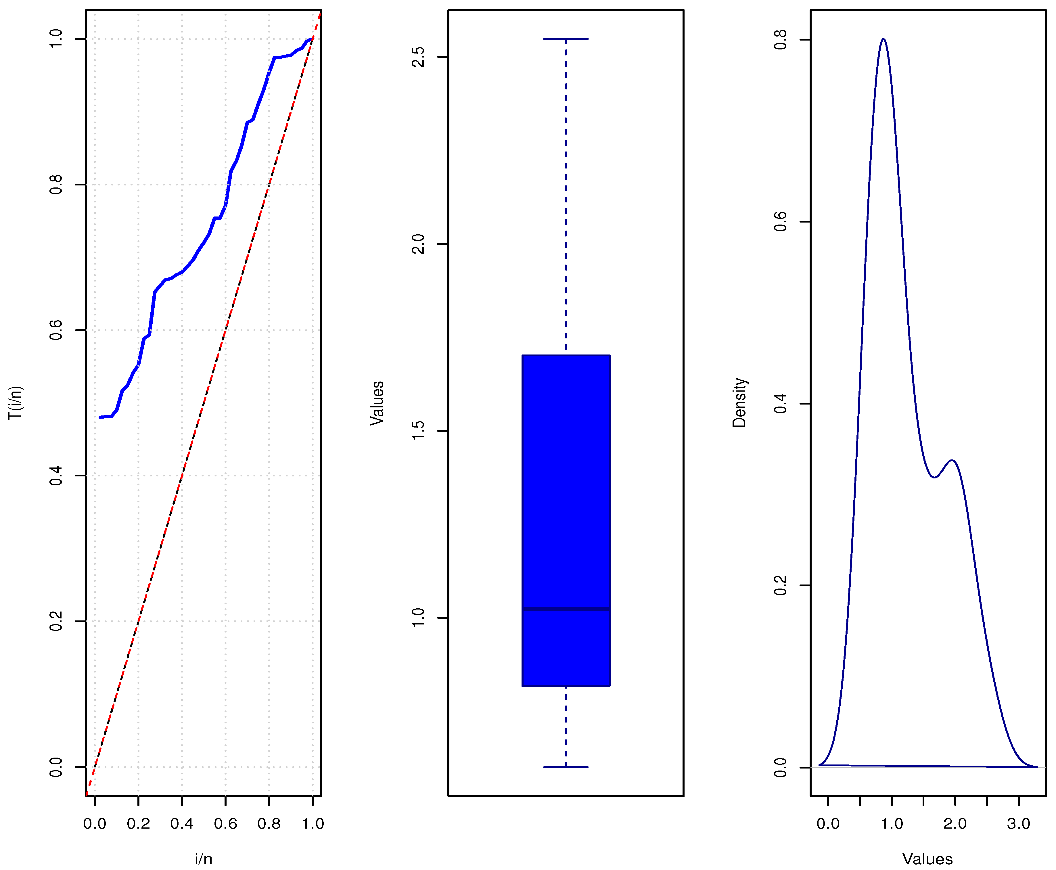
Table 8 and Figure 3 represent the descriptive statistical analysis and some graphical representations, including the TTT, box, and density plots, to illustrate the dataset used.

Table 8. Descriptive statistical analysis of the selected dataset.

Size	Mean	Median	SD	Min	Max	IQR	Skewness	Kurtosis
40	1.25	1.02	0.57	0.60	2.55	0.83	0.71	2.25

Figure 3. TTT, box, and density plots for the proposed dataset.

The descriptive statistics in Table 8 and the graphical representation in Figure 3 demonstrate a right-skewed distribution, characterized by a skewness of 0.71. The mean (1.25) being higher than the median (1.02) indicates the presence of some notably large values that pull the average upward. The data exhibits moderate dispersion, with a standard deviation of 0.57 and a coefficient of variation of 45.66%. The slightly platykurtic kurtosis of 2.25 suggests a distribution with fewer extreme values compared to a normal distribution.

To evaluate the adequacy and superiority of the proposed estimation methods under the I-PLD, we compare its performance with three related lifetime distributions: the Lindley distribution [23], the Inverse Lindley distribution [33], and the Inverse Weibull distribution [34]. Each of these models provides a different degree of flexibility in modeling positively skewed data, which allows us to assess the robustness and accuracy of the I-PLD fit. These models were fitted to the same real dataset, and their performances were evaluated using several goodness-of-fit criteria, including the Akaike Information Criterion (AIC), Corrected AIC (CAIC), Bayesian Information Criterion (BIC), Hannan–Quinn Information Criterion (HQIC), and the Kolmogorov–Smirnov (K–S) test.

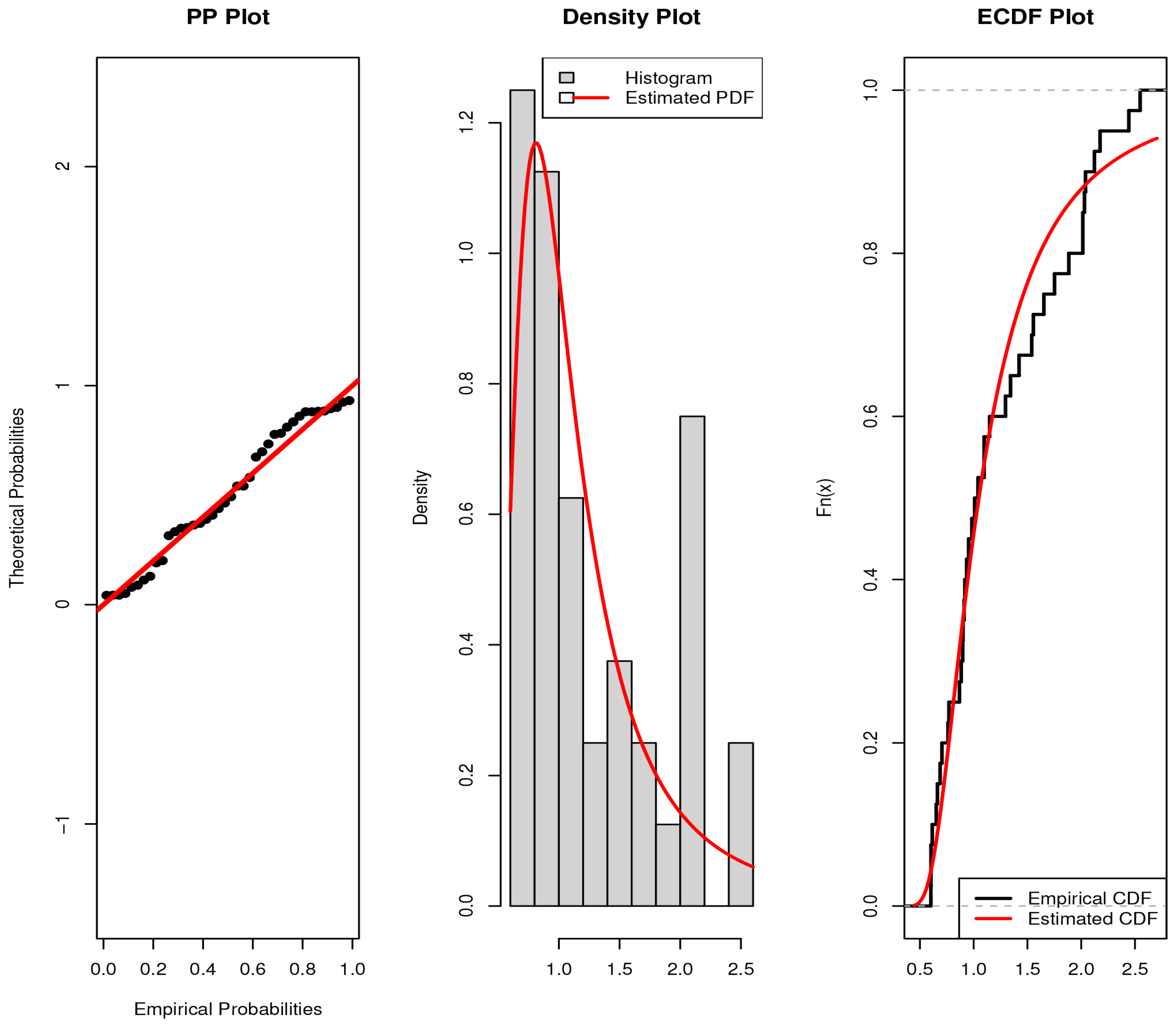
The results in Table 9 show that the IPLD provides the best fit to the data, as indicated by their lower AIC, CAIC, BIC, and HQIC values, and by their non-significant K–S test results (high p-values). Between these two, the IPLD demonstrates slightly better performance and stability, confirming its superiority and flexibility in modeling positively skewed lifetime data compared to the standard Lindley-type distributions. The graphical representation in Figure 4 provides visual confirmation of these statistical findings.

Table 9. Comparison of fitted models for the real dataset.

Statistic	IPLD	Lindley	Inverse Lindley	Inverse Weibull
W Statistic	0.0826	0.1758	0.0972	0.0811
A Statistic	0.6612	1.0575	0.6865	0.6430
K–S Statistic	0.1024	0.3438	0.2619	0.1035
K–S p-value	0.7959	0.00016	0.00828	0.7848
AIC	61.3547	93.5443	104.4534	60.9403
CAIC	61.6790	93.6495	104.5586	61.2646
BIC	64.7324	95.2331	106.1422	64.3181
HQIC	62.5759	94.1549	105.0640	62.1616

Figure 4. P-P, density and emperical CDF plots lots for the dataset.

To comprehensively examine the superiority of ranked set sampling over SRS across different estimation methods, an SRS sample of size 12 was chosen for comparability, while an RSS scheme was designed with a set size of 3 and four cycles to maintain the same total sample size. Assuming a perfect sampling design, an extensive evaluation was carried out using several goodness-of-fit statistics to assess the performance and reliability of each sampling approach. Specifically, we employed the Anderson–Darling test $A^{*}$, the Cramér-von Mises test $C^{*}$, and the Kolmogorov–Smirnov test $K^{*}$. These statistical measures were systematically applied to assess model fit and provide comparative insights into the effectiveness of RSS in capturing the underlying data distribution relative to SRS. A detailed comparison of the goodness-of-fit values for both sampling designs is presented in Table 10.

Table 10. Estimates and test statistics for each method under the two sampling schemes (SRS and RSS).

Method	Sampling	$\widehat{\mathit{\alpha }}$	$\widehat{\mathit{\beta }}$	${\mathit{A}}^{*}$	${\mathit{C}}^{*}$	${\mathit{K}}^{*}$	p-Value
MLE	SRS	4.2608	2.1232	22.4776	1.1928	0.3146	0.0007
	RSS	2.7212	1.2720	1.1726	0.1332	0.1169	0.6454
OLSE	SRS	2.9404	1.7829	6.3987	0.6300	0.2271	0.0323
	RSS	1.6713	1.2548	1.2061	0.1366	0.1415	0.3997
WLSE	SRS	3.0948	1.8497	8.0736	0.7307	0.2451	0.0163
	RSS	1.8401	1.2567	0.8286	0.0862	0.1218	0.5936
CVME	SRS	3.6223	1.9726	13.4570	0.9412	0.2790	0.0039
	RSS	2.1460	1.2533	0.5248	0.0564	0.0918	0.8886
MPSE	SRS	3.2835	1.8975	9.8602	0.8101	0.2585	0.0095
	RSS	1.9387	1.2715	0.6824	0.0703	0.1131	0.6856
ADE	SRS	3.5743	1.9508	12.7188	0.9100	0.2740	0.0049
	RSS	1.9801	1.2775	0.6396	0.0664	0.1096	0.7224
RTADE	SRS	3.4526	1.9129	11.2140	0.8498	0.2645	0.0074
	RSS	1.8857	1.2627	0.7530	0.0775	0.1176	0.6379
LTADE	SRS	3.8419	1.9579	15.0562	0.9595	0.2797	0.0038
	RSS	2.1647	1.2369	0.5221	0.0570	0.0887	0.9115
MSADE	SRS	3.3022	2.1078	13.4121	1.0725	0.2983	0.0016
	RSS	2.2708	1.1211	0.8176	0.1183	0.1184	0.6294
MSALDE	SRS	3.3614	2.0963	13.6203	1.0605	0.2973	0.0017
	RSS	2.3907	1.1984	0.6181	0.0800	0.1043	0.7773
MSSDE	SRS	2.8095	1.9136	7.6897	0.8065	0.2541	0.0114
	RSS	2.1106	1.0934	1.0517	0.1537	0.1402	0.4113
MSSLDE	SRS	3.5198	1.9024	11.5258	0.8475	0.2634	0.0078
	RSS	2.0642	1.2057	0.6029	0.0651	0.0945	0.8670
MSLDE	SRS	2.7897	1.9120	7.5892	0.8047	0.2534	0.0117
	RSS	2.1029	1.0955	1.0435	0.1515	0.1397	0.4158
KE	SRS	3.4779	1.9115	11.3693	0.8517	0.2646	0.0074
	RSS	2.0549	1.3886	0.8855	0.1186	0.1145	0.6712
ADLSOE	SRS	5.4097	1.9399	35.0314	1.2522	0.3060	0.0011
	RSS	2.9310	1.0423	2.0324	0.2909	0.1775	0.1605

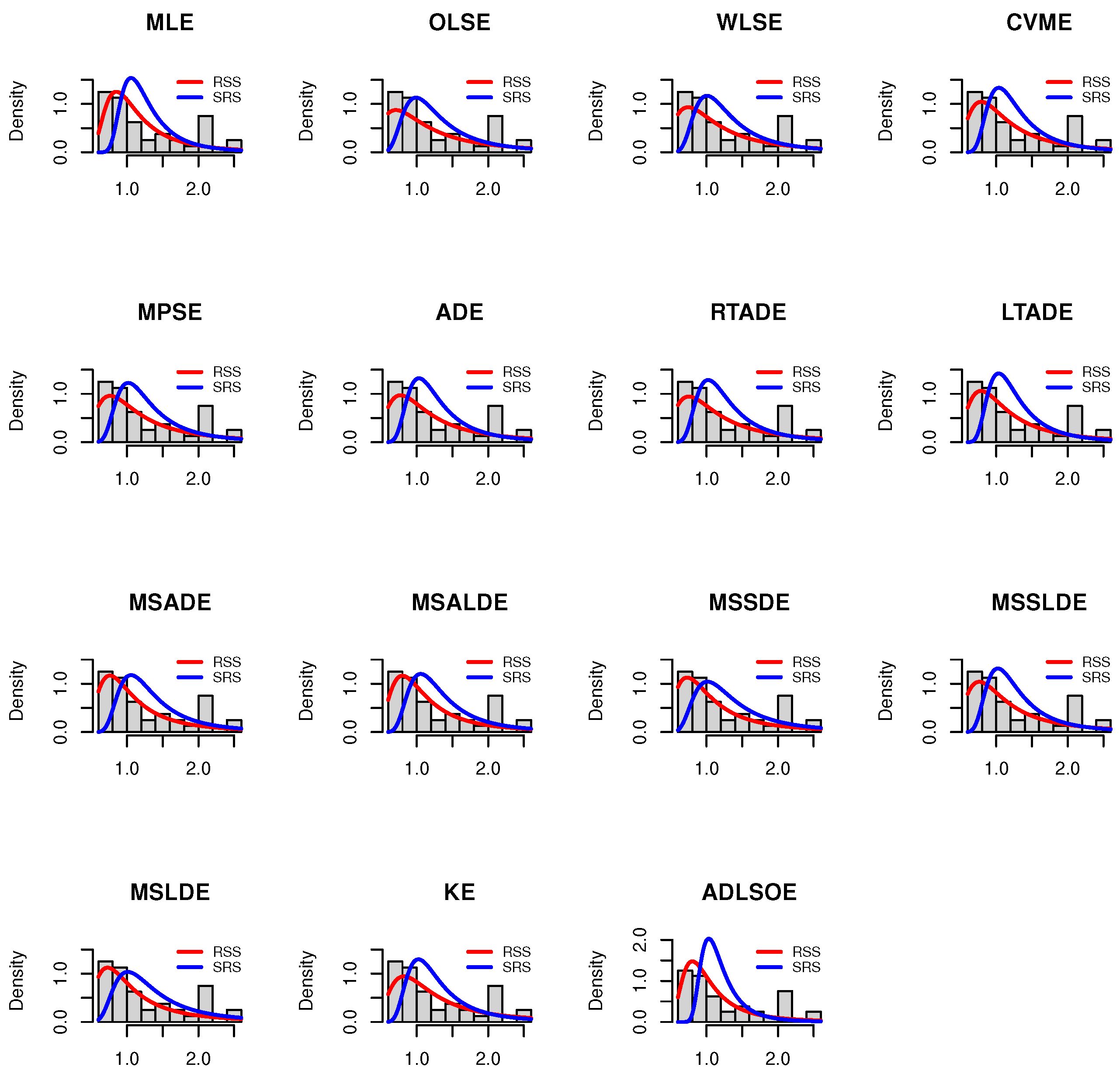
Table 10 revealed a consistent superiority of RSS over SRS across multiple estimation techniques. The RSS methodology demonstrated notably improved model fit, characterized by reduced $A^{*}$, $C^{*}$, and $K^{*}$ test values, coupled with elevated p-values. These empirical findings substantiate the theoretical advantages of RSS design. The graphical representations in Figure 5 and Figure 6 provide additional visual corroboration of these findings, reinforcing the robust performance of the RSS approach in statistical modeling.

Figure 5. Plots of the estimated PDFs of the I-PL distribution for the two sampling method for $m=3$ and $r=4$.

Figure 6. Plots of the estimated CDFs of the I-PL distribution for the two sampling method for $m=3$ and $r=4$.

5. Conclusions

This study provides strong evidence that ranked set sampling (RSS) outperforms simple random sampling (SRS) in estimating parameters of the inverse power Lindley distribution (IPLD). Through an extensive comparison of eleven estimation techniques, supported by large-scale simulations and empirical data, RSS consistently produced estimators with lower bias, smaller mean squared error, and improved mean relative error—all achieved without increasing the number of measurements. The results underline RSS’s intrinsic advantage in exploiting ranking information for greater estimation precision. While maximum likelihood estimation performed reliably, the most pronounced efficiency gains under RSS were seen in minimum distance estimators (based on Anderson–Darling and Cramér–von Mises criteria) and spacing-based approaches such as maximum product spacing and minimum spacing distance. Notably, MSSLDE and RTADE methods showed exceptional accuracy in estimating the scale parameter $\beta$, substantially reducing variance and MSE. These advantages were further validated using real failure time data, confirming the practical significance of RSS in applied settings. Given its efficiency, simplicity, and low implementation cost, RSS emerges as a valuable and practical tool for researchers and professionals in reliability engineering, survival analysis, and quality control. Future investigations may extend this work by developing new RSS variants, testing additional distributions, or broadening empirical applications to demonstrate its versatility in statistical inference.