The Density Function of the Stochastic SIQR Model with a Two-Parameters Mean-Reverting Process

Abstract

This study develops a stochastic SIQR epidemic model with mean-reverting Ornstein–Uhlenbeck (OU) processes for both transmission rate $\beta \left(t\right)$ and quarantine release rate $k\left(t\right)$; this is distinct from existing non-white-noise stochastic epidemic models, most of which focus on single-parameter perturbation or only stability analysis. It synchronously embeds OU dynamics into two core epidemic parameters to capture asynchronous fluctuations between infection spread and control measures. It adopts a rare measure solution framework to derive rigorous infection extinction conditions, linking OU’s ergodicity to long-term ${\beta }^{+}\left(t\right)$ averages. It obtains the explicit probability density function of the four-dimensional SIQR system, filling the gap of lacking quantifiable density dynamics in prior studies. Simulations validate that $R_0^d<1$ ensures almost sure extinction, while $R_0^e>1$ leads to stable stochastic persistence.

1. Introduction

Epidemiological modeling is key to understanding disease transmission, predicting outbreaks, and formulating control strategies [1]. Diekmann and Kretzschmar [2] linked transmission to demography; Feng and Thieme [3,4] refined endemic transitions; and Hethcote et al. [5] quantified quarantine efficacy. Traditional deterministic SIQR models [6,7] assume fixed parameters (e.g., constant$\beta ,k$) but fail to reflect real-world randomness—such as seasonal contact changes, policy adjustments, or medical resource fluctuations—requiring stochastic extensions [8].

$$\left\{\begin{array}{c}\dot{S}\left(t\right)=\Lambda -{\displaystyle \frac{\beta S\left(t\right)I\left(t\right)}{1+\alpha I\left(t\right)}}-\mu S\left(t\right),\hfill \\ \dot{I}\left(t\right)={\displaystyle \frac{\beta S\left(t\right)I\left(t\right)}{1+\alpha I\left(t\right)}}-(\delta +\gamma +\mu +{\mu }_1)I\left(t\right),\hfill \\ \dot{Q}\left(t\right)=\delta I\left(t\right)-(k+\mu +{\mu }_2)Q\left(t\right),\hfill \\ \dot{R}\left(t\right)=\gamma I\left(t\right)+kQ\left(t\right)-\mu R\left(t\right),\hfill \end{array}\right.$$

(1)

where all of the parameters are assumed to be positive and are defined in Table 1.

Table 1. The definitions of the parameters.

Parameter	Definition
$S\left(t\right)$	susceptible individuals
$I\left(t\right)$	infected individuals
$Q\left(t\right)$	quarantined individuals
$R\left(t\right)$	recovered individuals
$\Lambda$	the recruitment rate of susceptible
$\beta$	the average number of adequate contacts
$\mu$	the per capita natural mortality rate
$\delta$	the removal rate constant from the compartment I
k	the removal rate constant from the compartment Q
$\gamma$	the rate at which individuals recover from compartment I and move to compartment R
${\mu }_1$	the extra disease-related death rate constant in compartments I
${\mu }_2$	the extra disease-related death rate constant in compartments Q

Early stochastic models used white noise for tractability, but its memoryless, unbounded nature contradicts the mean-reverting trend of real epidemic parameters (e.g., $\beta$ stabilizes at a baseline post-outbreak). Ornstein–Uhlenbeck processes, which encode “fluctuation around a central value,” address this, yet existing OU-based studies have critical gaps.

Recent non-white noise stochastic epidemic research has limitations: (1) Quarantine/hospital compartment models focus on determinism, while Zhang et al. [6] only add white noise to $\beta$, ignoring k’s mean reversion. (2) White noise models [1,8] lack temporal correlation for parameters like seasonal $\beta$. (3) Non-Gaussian models [9] omit joint $\beta$(k) stochasticity and explicit compartment density functions.

To fill these gaps, this study develops a stochastic SIQR model with OU processes for both $\beta$ and $k\left(t\right)$ as follows:

$$\left\{\begin{array}{c}dS\left(t\right)=[\Lambda -{\displaystyle \frac{{\beta }^{+}\left(t\right)S\left(t\right)I\left(t\right)}{1+\alpha I\left(t\right)}}-\mu S\left(t\right)]dt,\hfill \\ dI\left(t\right)=[{\displaystyle \frac{{\beta }^{+}\left(t\right)S\left(t\right)I\left(t\right)}{1+\alpha I\left(t\right)}}-(\delta +\gamma +\mu +{\mu }_1)I\left(t\right)]dt,\hfill \\ dQ\left(t\right)=[\delta I\left(t\right)-(k^{+}\left(t\right)+\mu +{\mu }_2)Q\left(t\right)]dt,\hfill \\ dR\left(t\right)=[\gamma I\left(t\right)+k^{+}\left(t\right)Q\left(t\right)-\mu R\left(t\right)]dt,\hfill \\ d\beta \left(t\right)=\left[{\theta }_1(\overline{\beta }-\beta \left(t\right))\right]dt+{\sigma }_{1}d{B}_1\left(t\right),\hfill \\ dk\left(t\right)=\left[{\theta }_2(\overline{k}-k\left(t\right))\right]dt+{\sigma }_{2}d{B}_2\left(t\right).\hfill \end{array}\right.,$$

(2)

where ${\beta }^{+}\left(t\right)=max\{\beta \left(t\right),0\}$, and in the same way, $k^{+}\left(t\right)=max\{k\left(t\right),0\}$. In addition, we write $a\wedge b=min\{a,b\}$, and $a\bigvee b=max\{a,b\}$. The aim is to (1) capture asynchronous infection-control fluctuations; (2) derive an extinction threshold $R_0^d$ via OU’s ergodicity; (3) obtain the system’s explicit density function; and (4) validate thresholds $R_0^d/R_0^e$ via simulations.

This paper systematically investigates the dynamical behavior of stochastic SIQR models with mean-reverting process noise. The analysis is methodologically structured into four principal components: In Section 2, we establish the existence and uniqueness of the global mild solution for the considered system by applying the Banach fixed-point theorem. Subsequently, in Section 3, a Lyapunov function-based approach is employed to demonstrate the existence of a unique stationary distribution for the stochastic system (SI2). Through spectral analysis, we derive the explicit expression in Section 4, which enables us to characterize the extinction thresholds under different parameter regimes. Finally, extensive numerical simulations are conducted to validate the theoretical predictions through comparative analysis of stochastic trajectories and stationary distribution fitting.

2. Existence and Uniqueness of the Global Positive Solution of System (2)

Relevant basic knowledge about existence and uniqueness are found in reference [10], and the main conclusions are as follows.

Theorem 1.

Along with the initial value $(S\left(0\right),I\left(0\right),Q\left(0\right),R\left(0\right),\beta \left(0\right),k\left(0\right))\in {\mathbb{R}}_{+}^4\times {\mathbb{R}}^2$, there exists a unique solution $\left(S\right(t),I(t),Q(t),R(t),\beta (t),k(t\left)\right)$ of model (2) on $t\ge 0$ and the solution will remain in ${\mathbb{R}}_{+}^4\times {\mathbb{R}}^2$ with probability 1, that is, the solution $(S\left(t\right),I\left(t\right),Q\left(t\right),R\left(t\right),\beta \left(t\right),k\left(t\right))\in {\mathbb{R}}_{+}^4\times {\mathbb{R}}^2$ for all $t\ge 0$ a.s..

Proof. 

Due to [10], there is a unique local solution $(S\left(t\right),I\left(t\right),Q\left(t\right),R\left(t\right),\beta \left(t\right),k\left(t\right))\in {\mathbb{R}}_{+}^4\times {\mathbb{R}}^2$ on $t\in$(0, ${\tau }_0$) for any initial value, where ${\tau }_0$ is an explosion time. [11]. To prove that the local solution is global, we only need to prove ${\tau }_0=\infty$ a.s. Let ${\tau }_0$ be sufficiently large for every component of $(S\left(0\right),I\left(0\right),Q\left(0\right),R\left(0\right),e^{\beta \left(t\right)},e^{k\left(t\right))}$ lying within the interval $\left[{\displaystyle \frac{1}{{\tau }_0}},{\tau }_0\right]$. For each integer $n\ge n_0$, we define the stopping time

$$\begin{array}{cc}\hfill {\tau }_n=& inf\{0<t<{\tau }_0|\min \{S\left(t\right),I\left(t\right),Q\left(t\right),R\left(t\right),e^{\beta \left(t\right)},e^{k\left(t\right)}\}\le {\displaystyle \frac{1}{n}}\hfill \\ \hfill \mathrm{or}& \max \{S\left(t\right),I\left(t\right),Q\left(t\right),R\left(t\right),e^{\beta \left(t\right)},e^{k\left(t\right)}\}\ge n\},\hfill \end{array}$$

we set $inf\left\{\varnothing \right\}$ = ∞. Obviously, ${\tau }_n$ increases as $n\to \infty$. We set ${\tau }_{\infty }=li{m}_{n\to \infty }{\tau }_n$; thus, ${\tau }_{\infty }\le {\tau }_0$ a.s.; if we show that ${\tau }_{\infty }=\infty$ a.s., then ${\tau }_0=\infty$ a.s. If ${\tau }_{\infty }<\infty$ a.s., then there are two constants, $J>0$ and $\epsilon \in \left(0,1\right)$, such that $P\left\{{\tau }_{\infty }\le J\right\}>\epsilon .$ Therefore,

$$P\{{\tau }_n\le J\}\ge \epsilon ,foralln\ge n_1.$$

(3)

we have

$$d(S+I+Q+R)=[\Lambda -\mu (S+I+Q+R)-{\mu }_{1}I-{\mu }_{2}Q]dt\le [\Lambda -\mu (S+I+Q+R)]dt,$$

and then

$$S\left(t\right)+I\left(t\right)+Q\left(t\right)+R\left(t\right)\le \left\{\begin{array}{c}{\displaystyle \frac{\Lambda }{\mu }},S\left(0\right)+I\left(0\right)+Q\left(0\right)+R\left(0\right)\le {\displaystyle \frac{\Lambda }{\mu }}\hfill \\ S\left(0\right)+I\left(0\right)+R\left(0\right),S\left(0\right)+I\left(0\right)+Q\left(0\right)+R\left(0\right)>{\displaystyle \frac{\Lambda }{\mu }}\hfill \end{array}\right.$$

Define $W_0:{\mathbb{R}}_{+}^4\times {\mathbb{R}}^2\to {\mathbb{R}}_{+}$ as follows:

$$\begin{array}{cc}\hfill W_0(S\left(t\right),I\left(t\right),Q\left(t\right),R\left(t\right),\beta \left(t\right),k\left(t\right))=& S-1-lnS+I-1-lnI+Q-1-lnQ\hfill \\ & +R-1-lnR+{\displaystyle \frac{{\left(\beta \left(t\right)\right)}^2}{2}}+{\displaystyle \frac{{\left(k\left(t\right)\right)}^2}{2}}.\hfill \end{array}$$

By applying It$\widehat{o}$’s formula [12] to $W_0(S\left(t\right),I\left(t\right),Q\left(t\right),R\left(t\right),\beta \left(t\right),k\left(t\right))$, we have

$$d{W}_0=\mathcal{L}{W}_{0}dt+{\sigma }_1\beta \left(t\right)d{B}_1\left(t\right)+{\sigma }_{2}k\left(t\right)d{B}_2\left(t\right),$$

(4)

where

$$\begin{array}{cc}\hfill \mathcal{L}{W}_0=& \Lambda -\mu (S+I+Q+R)-{\mu }_{1}I-{\mu }_{2}Q-{\displaystyle \frac{\Lambda }{S}}+{\displaystyle \frac{{\beta }^{+}I}{1+\alpha I}}+\mu -{\displaystyle \frac{{\beta }^{+}S}{1+\alpha I}}\hfill \\ & +(\delta +\gamma +\mu +{\mu }_1)-{\displaystyle \frac{\delta I}{Q}}+(k^{+}+\mu +{\mu }_2)-{\displaystyle \frac{\gamma I+k^{+}Q}{R}}+\mu \hfill \\ & -{\theta }_1\beta \left(t\right)(\beta \left(t\right)-\overline{\beta })-{\theta }_{2}k\left(t\right)(k\left(t\right)-\overline{k})+{\displaystyle \frac{{\sigma }_1^2+{\sigma }_2^2}{2}}\hfill \\ \hfill \le & \Lambda +4\mu +\delta +\gamma +{\mu }_1+{\mu }_2+{\displaystyle \frac{{\sigma }_1^2+{\sigma }_2^2}{2}}+{\displaystyle \frac{\left|\beta \right(t\left)\right|}{\alpha }}+\left|k\left(t\right)\right|\hfill \\ & -{\theta }_1\beta {\left(t\right)}^2-{\theta }_{2}k{\left(t\right)}^2+{\theta }_1\overline{\beta }\beta \left(t\right)+{\theta }_2\overline{k}k\left(t\right)\hfill \\ \hfill \le & \Lambda +4\mu +\delta +\gamma +{\mu }_1+{\mu }_2+{\displaystyle \frac{{(\frac{1}{\alpha }+{\theta }_1\overline{\beta })}^2}{4{\theta }_1}}+{\displaystyle \frac{{(1+\overline{k}{\theta }_2)}^2}{4{\theta }_2}}\hfill \\ \hfill \le & k^s,\hfill \end{array}$$

where $k^s>0$; then, we have

$$\begin{array}{cc}\hfill E{W}_0& (S({\tau }_n\wedge J),I({\tau }_n\wedge J),Q({\tau }_n\wedge J),R({\tau }_n\wedge J),\beta ({\tau }_n\wedge J),k({\tau }_n\wedge J))\hfill \\ \hfill \le & W_0(S\left(0\right),I\left(0\right),Q\left(0\right),R\left(0\right),\beta \left(0\right),k\left(0\right))+k^{s}E({\tau }_n\wedge J)\hfill \\ \hfill \le & W_0(S\left(0\right),I\left(0\right),Q\left(0\right),R\left(0\right),\beta \left(0\right),k\left(0\right))+k^{s}J.\hfill \end{array}$$

Define ${\Omega }_n$ = $\left\{{\tau }_n\le T\right\}$ for $n\ge n_1$, therefore,

$$\begin{array}{cc}\hfill W_0& (S\left(0\right),I\left(0\right),Q\left(0\right),R\left(0\right),\beta \left(0\right),k\left(0\right))+k^{s}J\hfill \\ \hfill \ge & E\left[I_{{\Omega }_n}{W}_0(S({\tau }_n,\omega ),I({\tau }_n,\omega ),Q({\tau }_n,\omega ),R({\tau }_n,\omega ),\beta ({\tau }_n,\omega ),k({\tau }_n,\omega ))\right]\hfill \\ \hfill \ge & ϵ\left\{[n-1-lnn]\wedge [{\displaystyle \frac{1}{n}}-1+lnn]\wedge \left[{\displaystyle \frac{{(lnn)}^2}{2}}\right]\right\},\hfill \end{array}$$

where $I_{{\Omega }_n}$ is the indicator function of ${\Omega }_n$. Taking $n\to \infty$, we have

$$\infty >W_0(S\left(0\right),I\left(0\right),Q\left(0\right),R\left(0\right),\beta \left(0\right),k\left(0\right))+k^{s}J=\infty .$$

We have $(S\left(t\right),I\left(t\right),Q\left(t\right),R\left(t\right),\beta \left(t\right),k\left(t\right))\in {\mathbb{R}}_{+}^4\times {\mathbb{R}}^2$ for all $t\ge 0$ almost surely (a.s.). This completes the proof. □

Remark 1.

From Theorem 1, there is a unique global solution $(S\left(t\right),I\left(t\right),Q\left(t\right),R\left(t\right),\beta \left(t\right),k\left(t\right))\in {\mathbb{R}}_{+}^4\times {\mathbb{R}}^2$ a.s. of system (2). Therefore,

$$d(S+I+Q+R)\le [\Lambda -\mu (S+I+Q+R\left)\right]dt,$$

and

$$S\left(t\right)+I\left(t\right)+Q\left(t\right)+R\left(t\right)\le {\displaystyle \frac{\Lambda }{\mu }}+e^{-\mu t}(S\left(0\right)+E\left(0\right)+Q\left(0\right)+I\left(0\right)+R\left(0\right)-{\displaystyle \frac{\Lambda }{\mu }}).$$

If $S\left(0\right)+I\left(0\right)+Q\left(0\right)+R\left(0\right)\le {\displaystyle \frac{\Lambda }{\mu }}$, then $S\left(t\right)+I\left(t\right)+Q\left(t\right)+R\left(t\right)\le {\displaystyle \frac{\Lambda }{\mu }}$ a.s., so the region

$${\Gamma }_1=\left\{(S,I,Q,R,\beta ,K)\in {\mathbb{R}}_{+}^4\times {\mathbb{R}}^2:S>0,I>0,Q>0,R>0,0<S+I+Q+R\le {\displaystyle \frac{\Lambda }{\mu }}\right\}$$

is a positively invariant set of system (2) on ${\Gamma }_1$, and assuming $(S\left(0\right),I\left(0\right),Q\left(0\right),R\left(0\right),\beta \left(0\right),k\left(0\right))\in {\Gamma }_1$.

3. Existence of a Stationary Distribution of System (2)

Define a critical value

$$R_0^e=R_0-{\displaystyle \frac{\frac{\Lambda }{\mu }(1+\frac{\Lambda \overline{\beta }}{{\mu }^2}){\sigma }_1}{(\delta +\gamma +\mu +{\mu }_1)\sqrt{2{\theta }_1}}}.$$

Theorem 2.

Assuming $R_0^e>1$, the model (2) has a unique stationary distribution under $(S\left(0\right),I\left(0\right),Q\left(0\right),R\left(0\right),\beta \left(0\right),k\left(0\right))\in {\Gamma }_1$.

Proof. 

Define a $C^2$ function

$$\begin{array}{cc}\hfill V=& M_1(-lnI-\alpha I-e_{1}S+{\displaystyle \frac{e_2{(\beta \left(t\right)-\overline{\beta })}^2}{2}})-lnS-lnQ-lnR+(S+I+Q+R)\hfill \\ & +{\displaystyle \frac{\beta {\left(t\right)}^2}{2}}+{\displaystyle \frac{k{\left(t\right)}^2}{2}}\hfill \\ \hfill :=& M_0{V}_1-V_2-V_3-V_4+V_5+V_6+V_7,\hfill \end{array}$$

where $e_1$ and $e_2$ are both positive. The specific values of $e_1$ and $e_2$ will be given in the following proofs.

Applying It${\widehat{o}}^{\prime }s$ formula [13] to $V_1$, then we have

$$\begin{array}{cc}\hfill \mathcal{L}{V}_1=& -{\displaystyle \frac{{\beta }^{+}S}{1+\alpha I}}+(\delta +\gamma +\mu +{\mu }_1)-{\displaystyle \frac{\alpha {\beta }^{+}SI}{1+\alpha I}}+\alpha (\delta +\gamma +\mu +{\mu }_1)I-e_1\Lambda +{\displaystyle \frac{e_1{\beta }^{+}SI}{1+\alpha I}}\hfill \\ & +e_1\mu S-e_2{\theta }_1{(\beta \left(t\right)-\overline{\beta })}^2+{\displaystyle \frac{e_2{\sigma }_1^2}{2}}\hfill \\ \hfill \le & -\overline{\beta }S+|\overline{\beta }-\beta \left(t\right)|{\displaystyle \frac{\Lambda }{\mu }}+(\delta +\gamma +\mu +{\mu }_1)+\alpha (\delta +\gamma +\mu +{\mu }_1)I+e_1\mu S-e_1\Lambda \hfill \\ & +{\displaystyle \frac{e_1\overline{\beta }SI}{1+\alpha I}}+{\displaystyle \frac{|\beta \left(t\right)-\overline{\beta }|e_{1}SI}{1+\alpha I}}-e_2{\theta }_1{(\beta \left(t\right)-\overline{\beta })}^2+{\displaystyle \frac{e_2{\sigma }_1^2}{2}}.\hfill \end{array}$$

Let $e_1={\displaystyle \frac{\overline{\beta }}{\mu }}$, $e_2={\displaystyle \frac{\frac{\Lambda }{\mu }(1+\frac{\Lambda \overline{\beta }}{{\mu }^2})}{{\sigma }_1\sqrt{2{\theta }_1}}}$, then we have

$$\begin{array}{cc}\hfill \mathcal{L}{V}_1\le & |\overline{\beta }-\beta \left(t\right)|{\displaystyle \frac{\Lambda }{\mu }}-(R_0-1)(\delta +\gamma +\mu +{\mu }_1)+\left[{\displaystyle \frac{e_1\overline{\beta }\Lambda }{\mu }}+\alpha (\delta +\gamma +\mu +{\mu }_1)\right]I\hfill \\ & +|\overline{\beta }-\beta \left(t\right)|e_1{\left({\displaystyle \frac{\Lambda }{\mu }}\right)}^2-e_2{\theta }_1{(\beta \left(t\right)-\overline{\beta })}^2+{\displaystyle \frac{e_2{\sigma }_1^2}{2}}\hfill \\ \hfill \le & -(R_0-1)(\delta +\gamma +\mu +{\mu }_1)+\left[{\displaystyle \frac{e_1\overline{\beta }\Lambda }{\mu }}+\alpha (\delta +\gamma +\mu +{\mu }_1)\right]I+{\displaystyle \frac{{\left[\frac{\Lambda }{\mu }(1+\frac{\overline{\beta }\Lambda }{{\mu }^2})\right]}^2}{4{\theta }_1{e}_2}}+{\displaystyle \frac{e_2{\sigma }_1^2}{2}}\hfill \\ \hfill \le & -(R_0-1)(\delta +\gamma +\mu +{\mu }_1)+\left[{\displaystyle \frac{e_1\overline{\beta }\Lambda }{\mu }}+\alpha (\delta +\gamma +\mu +{\mu }_1)\right]I+{\displaystyle \frac{\frac{\Lambda }{\mu }(1+\frac{\Lambda \overline{\beta }}{{\mu }^2}){\sigma }_1}{\sqrt{2{\theta }_1}}}\hfill \\ \hfill \le & -(R_0^e-1)(\delta +\gamma +\mu +{\mu }_1)+\left[{\displaystyle \frac{e_1\overline{\beta }\Lambda }{\mu }}+\alpha (\delta +\gamma +\mu +{\mu }_1)\right]I,\hfill \end{array}$$

where

$$R_0^e=R_0-{\displaystyle \frac{\frac{\Lambda }{\mu }(1+\frac{\Lambda \overline{\beta }}{{\mu }^2}){\sigma }_1}{(\delta +\gamma +\mu +{\mu }_1)\sqrt{2{\theta }_1}}}.$$

In addition, applying the I$t{\widehat{o}}^{\prime }s$ formula to the others, we get

$$\begin{array}{cc}\hfill \mathcal{L}(-V_2)=& -{\displaystyle \frac{\Lambda }{S}}+{\displaystyle \frac{{\beta }^{+}I}{1+\alpha I}}+\mu \le -{\displaystyle \frac{\Lambda }{S}}+{\displaystyle \frac{\left|\beta \right(t\left)\right|\Lambda }{\mu }}+\mu ,\hfill \\ \hfill \mathcal{L}(-V_3)=& -{\displaystyle \frac{\delta I}{Q}}+(k^{+}+\mu +{\mu }_2),\hfill \\ \hfill \mathcal{L}(-V_4)=& -{\displaystyle \frac{\gamma I}{R}}-{\displaystyle \frac{k^{+}Q}{R}}+\mu \le -{\displaystyle \frac{\gamma I}{R}}+\mu ,\hfill \\ \hfill \mathcal{L}{V}_5=& \Lambda -\mu (S+I+Q+R)-{\mu }_{1}I-{\mu }_{2}Q\le \Lambda -\mu (S+I+Q+R),\hfill \\ \hfill \mathcal{L}{V}_6=& -{\theta }_1\beta \left(t\right)(\beta \left(t\right)-\overline{\beta })+{\displaystyle \frac{{\sigma }_1^2}{2}},\hfill \\ \hfill \mathcal{L}{V}_7=& -{\theta }_{2}k\left(t\right)(k\left(t\right)-\overline{k})+{\displaystyle \frac{{\sigma }_2^2}{2}}.\hfill \end{array}$$

Then we define a non-negative $C^2$-function $\tilde{V}(S,I,R,\beta ):{\mathbb{R}}_{+}^4\times {\mathbb{R}}^2\to {\mathbb{R}}_{+}^1$,

$$\tilde{V}(S,I,Q,R,\beta ,k)=V(S,I,Q,R,\beta ,k)-V_0,$$

(5)

where $V(S,I,Q,R,\beta ,k)$ has a minimum $V_0$. Applying the $It{\widehat{o}}^{\prime }s$ formula to $\tilde{V}(S,I,Q,R,\beta ,k)$, then, we have

$$\begin{array}{cc}\hfill \mathcal{L}\tilde{V}\le & -M_1(R_0^e-1)(\delta +\gamma +\mu +{\mu }_1)+M_1\left[{\displaystyle \frac{e_1\overline{\beta }\Lambda }{\mu }}+\alpha (\delta +\gamma +\mu +{\mu }_1)\right]I-{\displaystyle \frac{\Lambda }{S}}\hfill \\ & +{\displaystyle \frac{\left|\beta \right(t\left)\right|\Lambda }{\mu }}+\mu -{\displaystyle \frac{\delta I}{Q}}+(k^{+}+\mu +{\mu }_2)-{\displaystyle \frac{\gamma I}{R}}+\mu +\Lambda -\mu (S+I+Q+R)\hfill \\ & -{\theta }_1\beta \left(t\right)(\beta \left(t\right)-\overline{\beta })+{\displaystyle \frac{{\sigma }_1^2}{2}}-{\theta }_{2}k\left(t\right)(k\left(t\right)-\overline{k})+{\displaystyle \frac{{\sigma }_2^2}{2}}\hfill \\ \hfill \le & -M_1(R_0^e-1)(\delta +\gamma +\mu +{\mu }_1)+3\mu +{\mu }_2+\Lambda +{\displaystyle \frac{{\sigma }_1^2+{\sigma }_2^2}{2}}+{\displaystyle \frac{{(\frac{\Lambda }{\mu }+{\theta }_1\overline{\beta })}^2}{2{\theta }_1}}\hfill \\ & +{\displaystyle \frac{{(1+{\theta }_2\overline{k})}^2}{2{\theta }_2}}+M_1\left[{\displaystyle \frac{e_1\overline{\beta }\Lambda }{\mu }}+\alpha (\delta +\gamma +\mu +{\mu }_1)\right]I-{\displaystyle \frac{\Lambda }{S}}-{\displaystyle \frac{\delta I}{Q}}-{\displaystyle \frac{\gamma I}{R}}\hfill \\ & -\mu (S+I+Q+R)-{\displaystyle \frac{{\theta }_1\beta {\left(t\right)}^2}{2}}-{\displaystyle \frac{{\theta }_{2}k{\left(t\right)}^2}{2}},\hfill \end{array}$$

where $M_1$ is sufficiently large that it satisfies the following conditions

$$-M_1(R_0^e-1)(\delta +\gamma +\mu +{\mu }_1)+3\mu +{\mu }_2+\Lambda +{\displaystyle \frac{{\sigma }_1^2+{\sigma }_2^2}{2}}+{\displaystyle \frac{{(\frac{\Lambda }{\mu }+{\theta }_1\overline{\beta })}^2}{2{\theta }_1}}+{\displaystyle \frac{{(1+{\theta }_2\overline{k})}^2}{2{\theta }_2}}\le -2.$$

Construct a closed set $H_{ϵ}$ in the following form

$$H_{ϵ}=\left\{(S,I,Q,R,\beta ,k)\in {\Gamma }_1:S\ge ϵ,I\ge ϵ,Q\ge {ϵ}^{2}R\ge {ϵ}^2,S+I+Q+R\le {\displaystyle \frac{1}{ϵ}},\left|\beta \right|\le {\displaystyle \frac{1}{ϵ}},\left|k\right|\le {\displaystyle \frac{1}{ϵ}}\right\}.$$

where $ϵ$ is sufficiently small that satisfies the following conditions:

$$-2+M_1\left[{\displaystyle \frac{e_1\overline{\beta }\Lambda }{\mu }}+\alpha (\delta +\gamma +\mu +{\mu }_1)\right]ϵ\le -1,$$

(6)

$$-2+M_1\left[{\displaystyle \frac{e_1\overline{\beta }\Lambda }{\mu }}+\alpha (\delta +\gamma +\mu +{\mu }_1)\right]{\displaystyle \frac{\Lambda }{\mu }}-{\displaystyle \frac{min\{\Lambda ,\delta ,\gamma ,\mu \}}{ϵ}}\le -1,$$

(7)

$$-2+M_1\left[{\displaystyle \frac{e_1\overline{\beta }\Lambda }{\mu }}+\alpha (\delta +\gamma +\mu +{\mu }_1)\right]{\displaystyle \frac{\Lambda }{\mu }}-{\displaystyle \frac{min\{{\theta }_1,{\theta }_2\}}{2{ϵ}^2}}\le -1.$$

(8)

Then ${\Gamma }_1\setminus H_{ϵ}=H_{{ϵ}^1}^c\cup H_{{ϵ}^2}^c$…$\cup H_{{ϵ}^7}^c$, where

$$\begin{array}{cc}\hfill & H_{{ϵ}^1}^c=\left\{(S,I,Q,R,\beta ,k)\in {\Gamma }_1|S<ϵ\right\},H_{{ϵ}^2}^c=\left\{(S,I,Q,R,\beta ,k)\in {\Gamma }_1|I<ϵ\right\},\hfill \\ \hfill & H_{{ϵ}^3}^c=\left\{(S,I,Q,R,\beta ,k)\in {\Gamma }_1|I\ge ϵ,Q<{ϵ}^2\right\},H_{{ϵ}^4}^c=\left\{(S,I,Q,R,\beta ,k)\in {\Gamma }_1|I\ge ϵ,R<{ϵ}^2\right\},\hfill \\ \hfill & H_{{ϵ}^5}^c=\left\{(S,I,Q,R,\beta ,k)\in {\Gamma }_1|S+I+Q+R>{\displaystyle \frac{1}{ϵ}}\right\},H_{{ϵ}^6}^c=\left\{(S,I,Q,R,\beta ,k)\in {\Gamma }_1\left|\right|\beta |>{\displaystyle \frac{1}{ϵ}}\right\},\hfill \\ & H_{{ϵ}^7}^c=\left\{(S,I,Q,R,\beta ,k)\in {\Gamma }_1\left|\right|k|>{\displaystyle \frac{1}{ϵ}}\right\}.\hfill \end{array}$$

Case (1) If $(S,I,Q,R,\beta ,k)\in H_{{ϵ}^1}^c$, according to Equation (6), we have

$$-2+M_1\left[{\displaystyle \frac{e_1\overline{\beta }\Lambda }{\mu }}+\alpha (\delta +\gamma +\mu +{\mu }_1)\right]ϵ\le -1,$$

Case (2) If $(S,I,Q,R,\beta ,k)\in {\sum }_{i=2}^5{H}_{{ϵ}^i}^c$, from Equation (7), we get

$$-2+M_1\left[{\displaystyle \frac{e_1\overline{\beta }\Lambda }{\mu }}+\alpha (\delta +\gamma +\mu +{\mu }_1)\right]{\displaystyle \frac{\Lambda }{\mu }}-{\displaystyle \frac{min\{\Lambda ,\delta ,\gamma ,\mu \}}{ϵ}}\le -1,$$

Case (3) If $(S,I,Q,R,\beta ,k)\in {\sum }_{i=6}^7{H}_{{ϵ}^i}^c$, by Equation (8), we obtain

$$-2+M_1\left[{\displaystyle \frac{e_1\overline{\beta }\Lambda }{\mu }}+\alpha (\delta +\gamma +\mu +{\mu }_1)\right]{\displaystyle \frac{\Lambda }{\mu }}-{\displaystyle \frac{min\{{\theta }_1,{\theta }_2\}}{2{ϵ}^2}}\le -1.$$

Therefore, the global positive solution $\left(S\right(t),I(t),Q(t),R(t),\beta (t),k(t\left)\right)$ of system (2) converges as a stationary distribution $\pi$(·). This completes the proof of Theorem 2. □

4. Density Function and Extinction of System (2)

We define a quasi-equilibrium point $E_{*}=(S_{*},I_{*},Q_{*},R_{*},\overline{\beta },\overline{k})$ for system (2), which is determined by the following equation [4]

$$\left\{\begin{array}{c}\Lambda -{\displaystyle \frac{{\beta }^{+}\left(t\right)S_{*}\left(t\right)I_{*}\left(t\right)}{1+\alpha I_{*}\left(t\right)}}-\mu S_{*}\left(t\right)=0,\hfill \\ {\displaystyle \frac{{\beta }^{+}\left(t\right)S_{*}\left(t\right)I_{*}\left(t\right)}{1+\alpha I_{*}\left(t\right)}}-(\delta +\gamma +\mu +{\mu }_1)I_{*}\left(t\right)=0,\hfill \\ \delta I_{*}\left(t\right)-(k^{+}\left(t\right)+\mu +{\mu }_2)Q_{*}\left(t\right)=0,\hfill \\ \gamma I_{*}\left(t\right)+k^{+}\left(t\right)Q_{*}\left(t\right)-\mu R_{*}\left(t\right)=0,\hfill \\ {\theta }_1(\overline{\beta }-\beta \left(t\right))=0,\hfill \\ {\theta }_2(\overline{k}-k\left(t\right))=0.\hfill \end{array}\right.$$

(9)

where the definition of quasi-equilibrium is similar to that in Section 1.

Let $y_1=S-S_{*}$, $y_2=I-I_{*}$, $y_3=Q-Q_{*}$, $y_4=R-R_{*}$$y_5=\beta -\overline{\beta }$, $y_6=k-\overline{k}$; then we can get a linearized form of the system (2) as follows

$$\left\{\begin{array}{c}d{y}_1=(-a_{11}{y}_1-a_{12}{y}_2-a_{15}{y}_5)dt,\hfill \\ d{y}_2=(a_{21}{y}_1-a_{22}{y}_2+a_{15}{y}_5)dt,\hfill \\ d{y}_3=(a_{32}{y}_2-a_{33}{y}_3-a_{36}{y}_6)dt,\hfill \\ d{y}_4=(a_{42}{y}_2+a_{43}{y}_3-a_{44}{y}_4+a_{36}{y}_6),\hfill \\ d{y}_5=-a_{55}{y}_{5}dt+{\sigma }_{1}d{B}_1\left(t\right),\hfill \\ d{y}_6=-a_{66}{y}_{6}dt+{\sigma }_{2}d{B}_2\left(t\right).\hfill \end{array}\right.,$$

(10)

where

$$\begin{array}{cc}\hfill & a_{11}={\displaystyle \frac{\overline{\beta }{I}_{*}}{1+\alpha I_{*}}}+\mu >0,a_{12}={\displaystyle \frac{\overline{\beta }{S}_{*}(1+\alpha I_{*})-\alpha \overline{\beta }{S}_{*}{I}_{*}}{{(1+\alpha I_{*})}^2}}>0,a_{15}={\displaystyle \frac{S_{*}{I}_{*}}{1+\alpha I_{*}}}>0,\hfill \\ & a_{21}={\displaystyle \frac{\overline{\beta }{I}_{*}}{1+\alpha I_{*}}}>0,a_{22}=(\delta +\gamma +\mu +{\mu }_1)-{\displaystyle \frac{\overline{\beta }{S}_{*}(1+\alpha I_{*})-\alpha \overline{\beta }{S}_{*}{I}_{*}}{{(1+\alpha I_{*})}^2}}>0,a_{32}=\delta ,\hfill \\ & a_{33}=\overline{k}+\mu +{\mu }_2,a_{36}=Q_{*},a_{42}=\gamma ,a_{43}=\overline{k},\hfill \\ & a_{44}=\mu ,a_{55}={\theta }_1>0,a_{66}={\theta }_2>0.\hfill \end{array}$$

Theorem 3.

Around the equilibrium of approximately $E_{*}$, the stationary distribution has a normal density function $\Psi (S,I,Q,R,\beta ,k)$ along with initial value $(S\left(0\right),I\left(0\right),Q\left(0\right),R\left(0\right),\beta \left(0\right),k\left(0\right))\in {\Gamma }_1$. Then the specific form of the covariance matrix Σ is as follows.

$$\Sigma ={\xi }_1^2{\left(M_1{J}_5{J}_4{J}_3{J}_2{J}_1\right)}^{-1}{\Sigma }_a{\left[{\left(M_1{J}_5{J}_4{J}_3{J}_2{J}_1\right)}^{-1}\right]}^T+{\xi }_2^2{\left(M_2{J}_c{J}_b{J}_a\right)}^{-1}{\Sigma }_b{\left[{\left(M_2{J}_c{J}_b{J}_a\right)}^{-1}\right]}^T,$$

where

$${\xi }_1=a_{15}{w}_1{w}_3{\sigma }_1,{\xi }_2=a_{36}{w}_a{\sigma }_2.$$

$$J_1=\left(\begin{array}{cccccc}0& 0& 0& 0& 1& 0\\ 1& 0& 0& 0& 0& 0\\ 0& 1& 0& 0& 0& 0\\ 0& 0& 1& 0& 0& 0\\ 0& 0& 0& 1& 0& 0\\ 0& 0& 0& 0& 0& 1\end{array}\right),J_2=\left(\begin{array}{cccccc}1& 0& 0& 0& 0& 0\\ 0& 1& 0& 0& 0& 0\\ 0& 1& 1& 0& 0& 0\\ 0& 0& 0& 1& 0& 0\\ 0& 0& 0& 0& 1& 0\\ 0& 0& 0& 0& 0& 1\end{array}\right),$$

$$J_3=\left(\begin{array}{cccccc}1& 0& 0& 0& 0& 0\\ 0& 1& 0& 0& 0& 0\\ 0& 0& 1& 0& 0& 0\\ 0& 0& 0& 1& 0& 0\\ 0& 0& 0& -{\displaystyle \frac{a_{42}}{a_{32}}}& 1& 0\\ 0& 0& 0& 0& 0& 1\end{array}\right),J_4=\left(\begin{array}{cccccc}1& 0& 0& 0& 0& 0\\ 0& 1& 0& 0& 0& 0\\ 0& 0& 1& 0& 0& 0\\ 0& 0& {\displaystyle \frac{a_{32}}{w_1}}& 1& 0& 0\\ 0& 0& 0& 0& 1& 0\\ 0& 0& 0& 0& 0& 1\end{array}\right),$$

$$J_5=\left(\begin{array}{cccccc}1& 0& 0& 0& 0& 0\\ 0& 1& 0& 0& 0& 0\\ 0& 0& 1& 0& 0& 0\\ 0& 0& 0& 1& 0& 0\\ 0& 0& 0& -{\displaystyle \frac{w_4}{w_3}}& 1& 0\\ 0& 0& 0& 0& 0& 1\end{array}\right),J_a=\left(\begin{array}{cccccc}0& 0& 0& 0& 0& 1\\ 1& 0& 0& 0& 0& 0\\ 0& 1& 0& 0& 0& 0\\ 0& 0& 1& 0& 0& 0\\ 0& 0& 0& 1& 0& 0\\ 0& 0& 0& 0& 1& 0\end{array}\right),$$

$$J_b=\left(\begin{array}{cccccc}1& 0& 0& 0& 0& 0\\ 0& 1& 0& 0& 0& 0\\ 0& 0& 1& 0& 0& 0\\ 0& 0& 0& 1& 0& 0\\ 0& 0& 0& 1& 1& 0\\ 0& 0& 0& 0& 0& 1\end{array}\right),J_c=\left(\begin{array}{cccccc}1& 0& 0& 0& 0& 0\\ 0& 0& 0& 1& 0& 0\\ 0& 0& 0& 0& 1& 0\\ 0& 1& 0& 0& 0& 0\\ 0& 0& 1& 0& 0& 0\\ 0& 0& 0& 0& 0& 1\end{array}\right),$$

$$M_1=\left(\begin{array}{cccccc}{m}_1& m_2& m_3& m_4& 0& m_5\\ 0& w_1{w}_3& -w_3(a_{12}+a_{22}+a_{33})& a_{33}^2& 0& (a_{33}+a_{66})a_{36}\\ 0& 0& w_3& -a_{33}& 0& -a_{36}\\ 0& 0& 0& 1& 0& 0\\ 0& 0& 0& 0& 1& 0\\ 0& 0& 0& 0& 0& 1\end{array}\right),$$

where

$$\begin{array}{cc}\hfill & m_1=-a_{1}5w_1{w}_3,m_2=w_1{w}_3(a_{21}-a_{11}-a_{22}-a_{33}),\hfill \\ & m_3=-w_1{w}_3{a}_{12}+w_3(a_{12}+a_{22}+a_{33})(a_{12}+a_{22}),m_4=-a_{33}^3,\hfill \\ & m_5=-a_{33}^2{a}_{36}-a_{36}{a}_{66}(a_{33}+a_{66}).\hfill \end{array}$$

$$\begin{array}{cc}\hfill & M_2=\hfill \\ \hfill & \left(\begin{array}{cccccc}-a_{36}{w}_a& -(a_{33}+a_{44})w_a& a_{44}^2& (a_{32}+a_{42})a_{21}& d_0& (a_{32}+a_{42})a_{15}\\ 0& w_a& -a_{44}& 0& a_{32}+a_{42}& 0\\ 0& 0& 1& 0& 0& 0\\ 0& 0& 0& 1& 0& 0\\ 0& 0& 0& 0& 1& 0\\ 0& 0& 0& 0& 0& 1\end{array}\right),\hfill \end{array}$$

where $d_0=w_a{a}_{32}-(a_{32}+a_{42})(a_{22}+a_{44}).$

$${\Sigma }_a=\left(\begin{array}{cccc}{\displaystyle \frac{a_2{a}_3-a_1{a}_4}{2Q}}& 0& -{\displaystyle \frac{a_3}{2Q}}& 0\\ 0& {\displaystyle \frac{a_3}{2Q}}& 0& -{\displaystyle \frac{a_1}{2Q}}\\ -{\displaystyle \frac{a_3}{2Q}}& 0& {\displaystyle \frac{a_1}{2Q}}& 0\\ 0& -{\displaystyle \frac{a_1}{2Q}}& 0& {\displaystyle \frac{a_1{a}_2-a_3}{2a_{4}Q}}\end{array}\right),$$

$${\Sigma }_b=\left(\begin{array}{cccc}{\displaystyle \frac{b_2}{2(b_1{b}_2-b_3)}}& 0& -{\displaystyle \frac{1}{2(b_1{b}_2-b_3)}}& 0\\ 0& {\displaystyle \frac{1}{2(b_1{b}_2-b_3)}}& 0& 0\\ -{\displaystyle \frac{1}{2(b_1{b}_2-b_3)}}& 0& {\displaystyle \frac{b_1}{2b_3(b_1{b}_2-b_3)}}& 0\\ 0& 0& 0& 0\end{array}\right),$$

where $Q=a_1(a_2{a}_3-a_1{a}_4)-a_3^2$; the other parameters that are not defined will be given specific values in the proof below.

Proof. 

Let $Y={(y_1,y_2,y_3,y_4,y_5,y_6)}^T$, $B\left(t\right)={(0,0,0,0,B_1\left(t\right),B_2\left(t\right))}^T$, and

$$A=\left(\begin{array}{cccccc}-a_{11}& -a_{12}& 0& 0& -a_{15}& 0\\ a_{21}& -a_{22}& 0& 0& a_{15}& 0\\ 0& a_{32}& -a_{33}& 0& 0& -a_{36}\\ 0& a_{42}& a_{43}& -a_{44}& 0& a_{36}\\ 0& 0& 0& 0& -a_{55}& 0\\ 0& 0& 0& 0& 0& -a_{66}\end{array}\right),G=\left(\begin{array}{cccccc}0& 0& 0& 0& 0& 0\\ 0& 0& 0& 0& 0& 0\\ 0& 0& 0& 0& 0& 0\\ 0& 0& 0& 0& 0& 0\\ 0& 0& 0& 0& {\sigma }_1& 0\\ 0& 0& 0& 0& 0& {\sigma }_2\end{array}\right).$$

Then the corresponding linearized model (10) is written as $dY=AYdt+GdB\left(\right(t\left)\right)$. According to [13], the probability density function is as follows [14]:

$$\begin{array}{cc}\hfill & -{\displaystyle \frac{{\sigma }_1^2}{2}}{\displaystyle \frac{{\partial }^2\Psi }{\partial y_5^2}}-{\displaystyle \frac{{\sigma }_2^2}{2}}{\displaystyle \frac{{\partial }^2\Psi }{\partial y_6^2}}+{\displaystyle \frac{\partial }{\partial y_1}}[(-a_{11}{y}_1-a_{12}{y}_2-a_{15}{y}_5)\Psi ]+{\displaystyle \frac{\partial }{\partial y_2}}[(a_{21}{y}_1-a_{22}{y}_2+a_{15}{y}_5)\Psi ]\hfill \\ & +{\displaystyle \frac{\partial }{\partial y_3}}[(a_{32}{y}_2-a_{33}{y}_3-a_{36}{y}_6)\Psi ]+{\displaystyle \frac{\partial }{\partial y_4}}\left[(a_{42}{y}_2+a_{43}{y}_3-a_{44}{y}_4+a_{36}{y}_6)\right]\hfill \\ & +{\displaystyle \frac{\partial }{\partial y_5}}(-a_{55}{y}_5\Psi )+{\displaystyle \frac{\partial }{\partial z_1}}(-a_{66}{y}_6\Psi )=0.\hfill \end{array}$$

According to G is a constant matrix, we obtain

$$G^2+A\Sigma +\Sigma A^T=0.$$

Since [7], the above equation is written as

$$G_i^2+A{\Sigma }_i+{\Sigma }_i{A}^T=0(i=a,b),$$

where $G_a=(0,0,0,0,{\sigma }_1,0),G_b=(0,0,0,0,0,{\sigma }_2)$, $\Sigma ={\Sigma }_a+{\Sigma }_b$ and $G^2=G_a^2+G_b^2$.

Define

$$F=\left(\begin{array}{cccc}-a_{11}& -a_{12}& 0& 0\\ a_{21}& -a_{22}& 0& 0\\ 0& a_{32}& -a_{33}& 0\\ 0& a_{42}& a_{43}& -a_{44}\end{array}\right).$$

Before we can prove that $\Sigma$ is positive definite, the characteristic polynomial of the matrix F takes

$${\varphi }_F\left(\lambda \right)={\lambda }^4+q_1{\lambda }^3+q_2{\lambda }^2+q_3\lambda +q_4,$$

where

$$\begin{array}{cc}\hfill & q_1=a_{11}+a_{22}+a_{33}+a_{44}>0,\hfill \\ \hfill & q_2=(a_{11}+a_{22})(a_{33}+a_{44})+a_{33}{a}_{44}+a_{11}{a}_{22}+a_{12}{a}_{21}>0,\hfill \\ \hfill & q_3=(a_{11}+a_{22})a_{33}{a}_{44}+(a_{33}+a_{44})(a_{11}{a}_{22}+a_{12}{a}_{21})>0,\hfill \\ \hfill & q_4=(a_{11}{a}_{22}+a_{12}{a}_{21})a_{33}{a}_{44}>0,\hfill \\ \hfill & q_1(q_2{q}_3-q_1{q}_4)-q_3^2=q_1{q}_3(a_{11}+a_{22})(a_{33}+a_{44})+q_1{(a_{11}{a}_{22}+a_{12}{a}_{21})}^2(a_{33}+a_{44})\hfill \\ & +q_1(a_{11}+a_{22}){\left(a_{33}{a}_{44}\right)}^2>{(a_{11}{a}_{22}+a_{12}{a}_{21})}^2(a_{11}+a_{22})(a_{33}+a_{44})\hfill \\ & +(a_{33}+a_{44})(a_{11}+a_{22}){\left(a_{33}{a}_{44}\right)}^2>0\hfill \end{array}.$$

(11)

By the Routh–Hurwitz stability criterion [14], we know that the matrix F has all negative eigenvalues.

Step 1.Consider the equation

$$G_a^2+A{\Sigma }_a+{\Sigma }_a{A}^T=0.$$

(12)

Firstly, let $A_1=J_{1}A{J}_1^{-1}$; we have

$$A_1=\left(\begin{array}{cccccc}-a_{55}& 0& 0& 0& 0& 0\\ -a_{15}& -a_{11}& -a_{12}& 0& 0& 0\\ a_{15}& a_{21}& -a_{22}& 0& 0& 0\\ 0& 0& a_{32}& -a_{33}& 0& -a_{36}\\ 0& 0& a_{42}& a_{43}& -a_{44}& a_{36}\\ 0& 0& 0& 0& 0& -a_{66}\end{array}\right).$$

Next, let $A_2=J_3{J}_2{A}_1{\left(J_3{J}_2\right)}^{-1}$; we have

$$A_2=\left(\begin{array}{cccccc}-a_{55}& 0& 0& 0& 0& 0\\ -a_{15}& a_{12}-a_{11}& -a_{12}& 0& 0& 0\\ 0& w_1& -a_{12}-a_{22}& 0& 0& 0\\ 0& -a_{32}& a_{32}& -a_{33}& 0& -a_{36}\\ 0& 0& 0& w_2& -a_{44}& a_{36}+{\displaystyle \frac{a_{36}{a}_{42}}{a_{32}}}\\ 0& 0& 0& 0& 0& -a_{66}\end{array}\right),$$

where $w_1=a_{21}-a_{11}+a_{22}+a_{12}=\delta +\gamma +{\mu }_1\ne 0$, $w_2=a_{43}+{\displaystyle \frac{a_{33}{a}_{42}}{a_{32}}}-{\displaystyle \frac{a_{44}{a}_{42}}{a_{32}}}\ne 0$. Then we define $A_3=J_4{A}_2{J}_4^{-1}$; we have

$$A_3=\left(\begin{array}{cccccc}-a_{55}& 0& 0& 0& 0& 0\\ -a_{15}& a_{12}-a_{11}& -a_{12}& 0& 0& 0\\ 0& w_1& -a_{12}-a_{22}& 0& 0& 0\\ 0& 0& w_3& -a_{33}& 0& -a_{36}\\ 0& 0& w_4& w_2& -a_{44}& a_{36}+{\displaystyle \frac{a_{36}{a}_{42}}{a_{32}}}\\ 0& 0& 0& 0& 0& -a_{66}\end{array}\right),$$

where $w_3=a_{32}-{\displaystyle \frac{(a_{12}+a_{22})a_{32}}{w_1}}+{\displaystyle \frac{a_{32}{a}_{33}}{w_1}}\ne 0$, $w_4=-{\displaystyle \frac{w_2{a}_{32}}{w_1}}\ne 0$. Define $A_4=J_5{A}_3{J}_5^{-1}$; we obtain

$$A_4=\left(\begin{array}{cccccc}-a_{55}& 0& 0& 0& 0& 0\\ -a_{15}& a_{12}-a_{11}& -a_{12}& 0& 0& 0\\ 0& w_1& -a_{12}-a_{22}& 0& 0& 0\\ 0& 0& w_3& -a_{33}& 0& -a_{36}\\ 0& 0& 0& w_5& -a_{44}& w_6\\ 0& 0& 0& 0& 0& -a_{66}\end{array}\right),$$

where $w_5=w_2+{\displaystyle \frac{a_{33}{w}_4}{w_3}}-{\displaystyle \frac{a_{44}{w}_4}{w_3}}=0$, $w_6=a_{36}+{\displaystyle \frac{a_{36}{a}_{42}}{a_{32}}}+{\displaystyle \frac{a_{36}{w}_4}{w_3}}$. Let $A_5=M_1{A}_4{M}_1^{-1}$; then we obtain

$$A_5=\left(\begin{array}{cccccc}-a_1& -a_2& -a_3& -a_4& -a_5& -a_6\\ 1& 0& 0& 0& 0& 0\\ 0& 1& 0& 0& 0& 0\\ 0& 0& 1& 0& 0& 0\\ 0& 0& 0& 0& -a_{44}& w_6\\ 0& 0& 0& 0& 0& -a_{66}\end{array}\right),$$

where

$$\begin{array}{cc}\hfill & a_1=a_{11}+a_{22}+a_{33}+a_{55},\hfill \\ \hfill & a_2=(a_{11}+a_{22})(a_{33}+a_{55})+a_{33}{a}_{55}+a_{11}{a}_{22}+a_{12}{a}_{21},\hfill \\ \hfill & a_3=(a_{11}+a_{22})a_{33}{a}_{55}+(a_{33}+a_{55})(a_{11}{a}_{22}+a_{12}{a}_{21}),\hfill \\ \hfill & a_4=(a_{11}{a}_{22}+a_{12}{a}_{21})a_{33}{a}_{55}.\hfill \end{array}$$

For the values of $a_5$ and $a_6$ have no influence, we omit them here.

Therefore, the Equation (12) is equivalent to

$$\begin{array}{c}\hfill \left(M_1{J}_5{J}_4{J}_3{J}_2{J}_1\right)G_a^2{\left(M_1{J}_5{J}_4{J}_3{J}_2{J}_1\right)}^T+A_5\left[\left(M_1{J}_5{J}_4{J}_3{J}_2{J}_1\right){\Sigma }_a{\left(M_1{J}_5{J}_4{J}_3{J}_2{J}_1\right)}^T\right]\\ \hfill +\left[\left(M_1{J}_5{J}_4{J}_3{J}_2{J}_1\right){\Sigma }_a{\left(M_1{J}_5{J}_4{J}_3{J}_2{J}_1\right)}^T\right]A_5^T=0.\end{array}$$

(13)

Let ${\Sigma }_1={\xi }_1^{-2}\left(M_1{J}_5{J}_4{J}_3{J}_2{J}_1\right){\Sigma }_a{\left(M_1{J}_5{J}_4{J}_3{J}_2{J}_1\right)}^T$, where ${\xi }_1=a_{15}{w}_1{w}_3{\sigma }_1$; then, the above Equation (13) can be simplified as

$$G_0^2+A_5{\Sigma }_1+{\Sigma }_1{A}_5^T=0,$$

(14)

where $G_0=diag(1,0,0,0,0,0)$, by solving Equation (14), we have

$${\Sigma }_1=\left(\begin{array}{cccc}{\displaystyle \frac{a_2{a}_3-a_1{a}_4}{2Q}}& 0& -{\displaystyle \frac{a_3}{2Q}}& 0\\ 0& {\displaystyle \frac{a_3}{2Q}}& 0& -{\displaystyle \frac{a_1}{2Q}}\\ -{\displaystyle \frac{a_3}{2Q}}& 0& {\displaystyle \frac{a_1}{2Q}}& 0\\ 0& -{\displaystyle \frac{a_1}{2Q}}& 0& {\displaystyle \frac{a_1{a}_2-a_3}{2a_{4}Q}}\end{array}\right),$$

where $Q=a_1(a_2{a}_3-a_1{a}_4)-a_3^2$. Since the proof for $a_1(a_2{a}_3-a_1{a}_4)-a_3^2>0$ is similar to the proof for Equation (11), we omit it here. By the proof result of Zhou et al. [15], in Appendix A of his paper, we have that ${\Sigma }_1$ is semi-positive definite. Then, ${\Sigma }_a={\xi }_1^2{\left(M_1{J}_5{J}_4{J}_3{J}_2{J}_1\right)}^{-1}{\Sigma }_1{\left[{\left(M_1{J}_5{J}_4{J}_3{J}_2{J}_1\right)}^{-1}\right]}^T$ is also a semi-positive definite matrix. Furthermore, there exists a positive constant $f_1$ such that

$${\Sigma }_a\ge f_1\left(\begin{array}{cccccc}1& 0& 0& 0& 0& 0\\ 0& 1& 0& 0& 0& 0\\ 0& 0& 1& 0& 0& 0\\ 0& 0& 0& 0& 0& 0\\ 0& 0& 0& 0& 1& 0\\ 0& 0& 0& 0& 0& 0\end{array}\right).$$

For the following algebraic equation,

$$G_b^2+A{\Sigma }_b+{\Sigma }_b{A}^T=0.$$

(15)

Firstly, we define $B_1=J_{a}A{J}_a^{-1}$; then, we obtain

$$B_1=\left(\begin{array}{cccccc}-a_{66}& 0& 0& 0& 0& 0\\ 0& -a_{11}& -a_{12}& 0& 0& -a_{15}\\ 0& a_{21}& -a_{22}& 0& 0& a_{15}\\ -a_{36}& 0& a_{32}& -a_{33}& 0& 0\\ a_{36}& 0& a_{42}& a_{43}& -a_{44}& 0\\ 0& 0& 0& 0& 0& -a_{55}\end{array}\right).$$

Define $B_2=J_b{B}_1{J}_b^{-1}$; then, we have

$$B_2=\left(\begin{array}{cccccc}-a_{66}& 0& 0& 0& 0& 0\\ 0& -a_{11}& -a_{12}& 0& 0& -a_{15}\\ 0& a_{21}& -a_{22}& 0& 0& a_{15}\\ -a_{36}& 0& a_{32}& -a_{33}& 0& 0\\ 0& 0& a_{42}+a_{32}& w_a& -a_{44}& 0\\ 0& 0& 0& 0& 0& -a_{55}\end{array}\right),$$

where $w_a=a_{43}-a_{33}+a_{44}=-{\mu }_2\ne 0$, let $B_3=J_c{B}_2{J}_c^{-1}$; we get

$$B_3=\left(\begin{array}{cccccc}-a_{66}& 0& 0& 0& 0& 0\\ -a_{36}& -a_{33}& 0& 0& a_{32}& 0\\ 0& w_a& -a_{44}& 0& a_{32}+a_{42}& 0\\ 0& 0& 0& -a_{11}& -a_{12}& -a_{15}\\ 0& 0& 0& a_{21}& -a_{22}& a_{15}\\ 0& 0& 0& 0& 0& -a_{55}\end{array}\right).$$

Finally, let $B_4=M_2{B}_3{M}_2^{-1}$; then we obtain

$$B_4=\left(\begin{array}{cccccc}-b_1& -b_2& -b_3& -b_4& -b_5& -b_6\\ 1& 0& 0& 0& 0& 0\\ 0& 1& 0& 0& 0& 0\\ 0& 0& 0& -a_{11}& -a_{12}& -a_{15}\\ 0& 0& 0& a_{21}& -a_{22}& a_{15}\\ 0& 0& 0& 0& 0& -a_{55}\end{array}\right),$$

where

$$\begin{array}{cc}\hfill & b_1=a_{33}+a_{44}+a_{66}>0,\hfill \\ \hfill & b_2=a_{33}{a}_{44}+a_{44}{a}_{66}+a_{33}{a}_{66}>0,\hfill \\ \hfill & b_3=a_{33}{a}_{44}{a}_{66}>0,\hfill \\ \hfill & b_1{b}_2-b_3>(a_{33}+a_{44})b_2>0.\hfill \end{array}$$

Similarly, we omit $b_4$, $b_5$ and $b_6$ here. Therefore, Equation (15) is equivalent to

$$\begin{array}{c}\hfill \left(M_2{J}_c{J}_b{J}_a\right)G_b^2{\left(M_2{J}_c{J}_b{J}_a\right)}^T+B_4\left[\left(M_2{J}_c{J}_b{J}_a\right){\Sigma }_B{\left(M_2{J}_c{J}_b{J}_a\right)}^T\right]+\left[\left(M_2{J}_c{J}_b{J}_a\right){\Sigma }_b{\left(M_2{J}_c{J}_b{J}_a\right)}^T\right]B_4^T=0.\end{array}$$

(16)

Let ${\Sigma }_2={\xi }_2^{-2}\left(M_2{J}_c{J}_b{J}_a\right){\Sigma }_b{\left(M_2{J}_c{J}_b{J}_a\right)}^T$, where ${\xi }_2=a_{36}{w}_a{\sigma }_2$, then the above Equation (16) can be equivalent to

$$G_0^2+B_4{\Sigma }_2+{\Sigma }_2{B}_4^T=0.$$

(17)

By solving Equation (17) above, we obtain

$${\Sigma }_2=\left(\begin{array}{ccccc}-{\displaystyle \frac{b_2}{2(b_3-b_1{b}_2)}}& 0& {\displaystyle \frac{1}{2(b_3-b_1{b}_2)}}& 0& 0\\ 0& -{\displaystyle \frac{1}{2(b_3-b_1{b}_2)}}& 0& 0& 0\\ {\displaystyle \frac{1}{2(b_3-b_1{b}_2)}}& 0& -{\displaystyle \frac{b_1}{2(b_3-b_1{b}_2)}}& 0& 0\\ 0& 0& 0& 0& 0\\ 0& 0& 0& 0& 0\end{array}\right).$$

According to $b_1{b}_2-b_3>0$, by the proof result of Zhou et al. [15], in the Appendix A of his paper, we have that ${\Sigma }_1$ is semi-positive definite. Then, ${\Sigma }_b={\xi }_2^2{\left(M_2{J}_c{J}_b{J}_a\right)}^{-1}{\Sigma }_2{\left[{\left(M_2{J}_c{J}_b{J}_a\right)}^{-1}\right]}^T$ is also a semi-positive matrix. Furthermore, there exists a positive number $f_2$ satisfying

$${\Sigma }_b\ge f_2\left(\begin{array}{cccccc}0& 0& 0& 0& 0& 0\\ 0& 0& 0& 0& 0& 0\\ 0& 0& 1& 0& 0& 0\\ 0& 0& 0& 1& 0& 0\\ 0& 0& 0& 0& 0& 0\\ 0& 0& 0& 0& 0& 1\end{array}\right).$$

Then, the covariance matrix

$$\begin{array}{cc}\hfill \Sigma ={\Sigma }_a+{\Sigma }_b& \ge f_1\left(\begin{array}{cccccc}1& 0& 0& 0& 0& 0\\ 0& 1& 0& 0& 0& 0\\ 0& 0& 1& 0& 0& 0\\ 0& 0& 0& 0& 0& 0\\ 0& 0& 0& 0& 1& 0\\ 0& 0& 0& 0& 0& 0\end{array}\right)+f_2\left(\begin{array}{cccccc}0& 0& 0& 0& 0& 0\\ 0& 0& 0& 0& 0& 0\\ 0& 0& 1& 0& 0& 0\\ 0& 0& 0& 1& 0& 0\\ 0& 0& 0& 0& 0& 0\\ 0& 0& 0& 0& 0& 1\end{array}\right)\hfill \\ \hfill & \ge (f_1\wedge f_2)\left(\begin{array}{cccccc}1& 0& 0& 0& 0& 0\\ 0& 1& 0& 0& 0& 0\\ 0& 0& 1& 0& 0& 0\\ 0& 0& 0& 1& 0& 0\\ 0& 0& 0& 0& 1& 0\\ 0& 0& 0& 0& 0& 1\end{array}\right).\hfill \end{array}$$

Furthermore, the normal density function exists around $E_{*}$. □

Theorem 4.

Along with the initial value $(S\left(0\right),I\left(0\right),Q\left(0\right),R\left(0\right),\beta \left(0\right),k\left(0\right))\in {\Gamma }_1$, if $R_0^d<1$, then the solution $\left(S\right(t),I(t),Q(t),R(t),\beta (t),k(t\left)\right)$ of system (2) converges as

$$\underset{t\to \infty }{lim}sup{\displaystyle \frac{lnI\left(t\right)}{t}}\le (\delta +\gamma +\mu +{\mu }_1)(R_0^d-1)<0,a.s.$$

where

$$R_0^d={\displaystyle \frac{\left[\overline{\beta }\Phi \left(\frac{\overline{\beta }\sqrt{2{\theta }_1}}{{\sigma }_1}\right)+\frac{{\sigma }_1}{2\sqrt{{\theta }_1\pi }}{e}^{-\frac{{\overline{\beta }}^2{\theta }_1}{{\sigma }_1^2}}\right]\Lambda }{\mu (\delta +\gamma +\mu +{\mu }_1)}},$$

Proof. 

According to It$\widehat{o}$’s formula, we have

$$\begin{array}{cc}\hfill dlnI\left(t\right)=& \left[{\displaystyle \frac{{\beta }^{+}S}{1+\alpha I}}-(\delta +\gamma +\mu +{\mu }_1)\right]dt\hfill \\ \hfill \le & [{\beta }^{+}S-(\delta +\gamma +\mu +{\mu }_1)]dt\hfill \\ \hfill \le & [{\displaystyle \frac{{\beta }^{+}\Lambda }{\mu }}-(\delta +\gamma +\mu +{\mu }_1)]dt.\hfill \end{array}$$

Integrating this from 0 to t and dividing by t leads to

$$\begin{array}{cc}\hfill {\displaystyle \frac{lnI\left(t\right)-lnI\left(0\right)}{t}}\le & {\displaystyle \frac{1}{t}}{\int }_0^t[{\displaystyle \frac{{\beta }^{+}\left(s\right)\Lambda }{\mu }}-(\delta +\gamma +\mu +{\mu }_1)]ds\hfill \\ \hfill =& {\displaystyle \frac{\Lambda }{\mu t}}{\int }_0^t{\beta }^{+}\left(s\right)ds-(\delta +\gamma +\mu +{\mu }_1).\hfill \end{array}$$

By [6], we obtain

$$\begin{array}{cc}\hfill \underset{t\to \infty }{lim}{\displaystyle \frac{1}{t}}{\int }_0^t{\beta }^{+}\left(s\right)ds={\int }_0^{\infty }x{\displaystyle \frac{\sqrt{{\theta }_1}}{\sqrt{\pi }{\sigma }_1}}{e}^{-{\displaystyle \frac{{\theta }_1{x}^2}{{\sigma }_1^2}}}dx& ={\displaystyle \frac{{\sigma }_1}{2\sqrt{{\theta }_1\pi }}}{e}^{-{\displaystyle \frac{{\overline{\beta }}^2{\theta }_1}{{\sigma }_1^2}}}+\overline{\beta }\left[\Phi (\infty )-\Phi \left(-{\displaystyle \frac{\overline{\beta }\sqrt{2{\theta }_1}}{{\sigma }_1}}\right)\right]\hfill \\ & =\overline{\beta }\Phi \left({\displaystyle \frac{\overline{\beta }\sqrt{2{\theta }_1}}{{\sigma }_1}}\right)+{\displaystyle \frac{{\sigma }_1}{2\sqrt{{\theta }_1\pi }}}{e}^{-{\displaystyle \frac{{\overline{\beta }}^2{\theta }_1}{{\sigma }_1^2}}},\hfill \end{array}$$

where $\Phi \left(x\right)={\int }_{-\infty }^x{\displaystyle \frac{1}{\sqrt{2\pi }}}{e}^{-{\displaystyle \frac{v^2}{2}}}dv$, because of $\underset{t\to \infty }{lim}{\displaystyle \frac{lnI\left(0\right)}{t}}=0$; then, we have

$$\underset{t\to \infty }{lim}sup{\displaystyle \frac{lnI\left(t\right)}{t}}\le (\delta +\gamma +\mu +{\mu }_1)(R_0^d-1)<0,a.s.$$

where

$$R_0^d={\displaystyle \frac{\left[\overline{\beta }\Phi \left(\frac{\overline{\beta }\sqrt{2{\theta }_1}}{{\sigma }_1}\right)+\frac{{\sigma }_1}{2\sqrt{{\theta }_1\pi }}{e}^{-\frac{{\overline{\beta }}^2{\theta }_1}{{\sigma }_1^2}}\right]\Lambda }{\mu (\delta +\gamma +\mu +{\mu }_1)}},$$

The proof is completed. □

5. Numerical Simulations

We study the spread of disease through numerical simulations. Along [6,8], the corresponding discretization equation of model (2) is given by

$$\left\{\begin{array}{c}{S}_{i+1}=S_i+[\Lambda -{\displaystyle \frac{{\beta }_i{S}_i{I}_i}{1+\alpha I_i}}-\mu S_i]\Delta t,\hfill \\ I_{i+1}=I_i+[{\displaystyle \frac{{\beta }_i{S}_i{I}_i}{1+\alpha I_i}}-(\delta +\gamma +\mu +{\mu }_1)I_i]\Delta t,\hfill \\ Q_{i+1}=Q_i+[\delta I_i-(k_i+\mu +{\mu }_2)Q_i]\Delta t,\hfill \\ R_{i+1}=R_i+[\gamma I_i+k_i{Q}_i-\mu R_i]\Delta t,\hfill \\ {\beta }_{i+1}={\beta }_i+{\theta }_1(\overline{\beta }-{\beta }_i)\Delta t+{\sigma }_1{\iota }_i\sqrt{\Delta t}+{\displaystyle \frac{{\sigma }_1^2}{2}}({\iota }_i^2-1)\Delta t,\hfill \\ k_{i+1}=k_i+{\theta }_2(k-k_i)\Delta t+{\sigma }_2{\zeta }_i\sqrt{\Delta }+{\displaystyle \frac{{\sigma }_2^2}{2}}({\zeta }_i^2-1)\Delta t,\hfill \end{array}\right.$$

(18)

where $\Delta t>0$.

Let the parameters $\Lambda =0.8$, $\mu =0.5$, $\gamma =0.5$, $\delta =0.5$, ${\mu }_1=0.1$, ${\mu }_2=0.3$, $\overline{\beta }=5$, $\overline{k}=0.2$, $\alpha =1$, and let the stochastic perturbations ${\sigma }_1=\sqrt{0.05}$, ${\theta }_1=0.5$, ${\sigma }_2=\sqrt{0.05}$, ${\theta }_2=0.5$. According to Theorem 2, which we have already proven, System (10) has the corresponding conclusion, which can be shown in Figure 1.

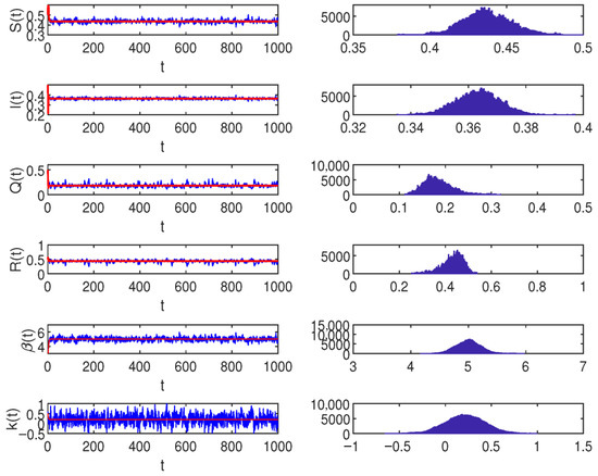
Figure 1. When $R_0^d=1.1987>1$, the blue lines represent the simulations under Ornstein–Uhlenbeck process on the left. On the right, the frequency histogram and marginal density function curve of $\Lambda =0.8$, $\mu =0.5$, $\gamma =0.5$, $\delta =0.5$, ${\mu }_1=0.1$, ${\mu }_2=0.3$, $\overline{\beta }=5$, $\overline{k}=0.2$, $\alpha =1$, and let the stochastic perturbations ${\sigma }_1=\sqrt{0.05}$, ${\theta }_1=0.5$, ${\sigma }_2=\sqrt{0.05}$, ${\theta }_2=0.5$ in the model (2).

Consider the main parameters $\Lambda =0.8$, $\mu =0.5$, $\gamma =0.5$, $\delta =0.5$, ${\mu }_1=0.1$, ${\mu }_2=0.3$, $\overline{\beta }=5$, $\overline{k}=0.2$, $\alpha =1$, and similarly let the stochastic perturbations ${\sigma }_1=\sqrt{0.05}$, ${\theta }_1=0.5$, ${\sigma }_2=\sqrt{0.05}$, ${\theta }_2=0.5$. According to the results already given in Theorem 4, the infected individuals in system (2) will be extinct, as shown in Figure 2.

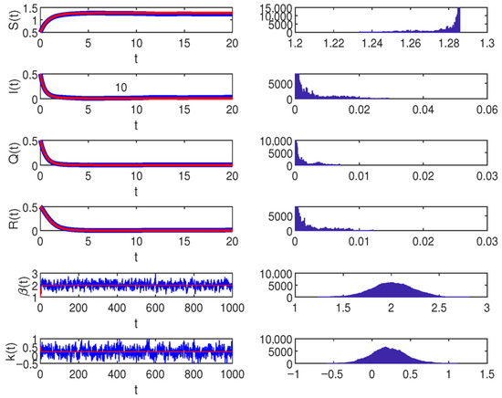
Figure 2. When $R_0^d=0.9986<1$, the blue lines show the simulations under the Ornstein–Uhlenbeck process on the left. The right figure presents the density properties with $\Lambda =0.8$, $\mu =0.5$, $\gamma =0.5$, $\delta =0.5$, ${\mu }_1=0.1$, ${\mu }_2=0.3$, $\overline{\beta }=5$, $\overline{k}=0.2$, $\alpha =1$, and similarly, let the stochastic perturbations ${\sigma }_1=\sqrt{0.05}$, ${\theta }_1=0.5$, ${\sigma }_2=\sqrt{0.05}$, ${\theta }_2=0.5$ in model (2).

Therefore, the blue shows the simulations of the model (2) and the red indicates the simulation of the system (1). The figure on the right represents the density of the model (2). In Figure 2, when $R_0^d<1$. This similarly means that the system (2) will be extinct.

In system (2), parameters $\Lambda$, $\overline{\beta }$, and $\mu$ play a key role in numerical simulations. By analyzing each of them individually, examples can be found in Figure 3, Figure 4 and Figure 5.

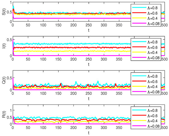
Figure 3. Numerical simulations of the solution S(t), I(t), Q(t) and R(t) in model (2) under the different $\Lambda =0.8$, $\Lambda =0.6$, $\Lambda =0.4$, and $\Lambda =0.08$ values, respectively.

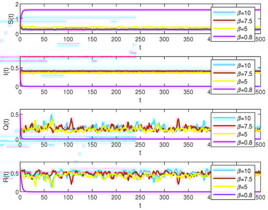
Figure 4. Numerical simulations of the solutions S(t), I(t), Q(t) and R(t) in system (2) under the different $\overline{\beta }$ values, $\overline{\beta }=10$, $\overline{\beta }=7.5$, $\overline{\beta }=5$, $\overline{\beta }=0.8$ values, respectively.

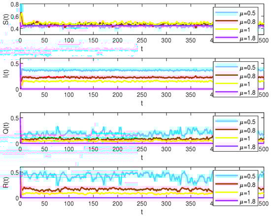
Figure 5. Numerical simulations of the solution S(t), I(t), Q(t) and R(t) in model (2) under the different $\mu$ values, $\mu =0.5$, $\mu =0.8$, $\mu =1$, $\mu =1.8$, respectively.

Let the main parameters $\mu =0.5$, $\gamma =0.5$, $\delta =0.5$, ${\mu }_1=0.1$, ${\mu }_2=0.3$, $\overline{\beta }=5$, $\overline{k}=0.2$, $\alpha =1$, and let the stochastic perturbations ${\sigma }_1=\sqrt{0.05}$, ${\theta }_1=0.5$, ${\sigma }_2=\sqrt{0.05}$, ${\theta }_2=0.5$. And

$$\begin{array}{cc}\hfill & R_0^e=1.1987>1,when\Lambda =0.8,\hfill \\ \hfill & R_0^e=1.5698>1,when\Lambda =0.6,\hfill \\ \hfill & R_0^e=1.4938>1,when\Lambda =0.4,\hfill \\ \hfill & R_0^d=0.5000<1,when\Lambda =0.08,\hfill \end{array}$$

which represents that for $\Lambda =0.8$, $\Lambda =0.6$, $\Lambda =0.4$, the diseases will persist but will be extinct when $\Lambda =0.08$ as in Figure 3.

With the data $\Lambda =0.8$, $\mu =0.5$, $\gamma =0.5$, $\delta =0.5$, ${\mu }_1=0.1$, ${\mu }_2=0.3$, $\overline{k}=0.2$, $\alpha =1$, let the stochastic perturbations ${\sigma }_1=\sqrt{0.05}$, ${\theta }_1=0.5$, ${\sigma }_2=\sqrt{0.05}$, ${\theta }_2=0.5$. And

$$\begin{array}{cc}\hfill & R_0^e=2.6210>1,when\overline{\beta }=10,\hfill \\ \hfill & R_0^e=1.9098>1,when\overline{\beta }=7.5,\hfill \\ \hfill & R_0^e=1.1987>1,when\overline{\beta }=5,\hfill \\ \hfill & R_0^d=0.8001<1,when\overline{\beta }=0.8,\hfill \end{array}$$

which illustrates that the diseases will exist when $\overline{\beta }=10$, $\overline{\beta }=7.5$, $\overline{\beta }=5$ but will be extinct when $\overline{\beta }=0.8$, as in Figure 4.

Consider the parameters $\Lambda =0.8$, $\gamma =0.5$, $\delta =0.5$, ${\mu }_1=0.1$, ${\mu }_2=0.3$, $\overline{\beta }=5$, $\overline{k}=0.2$, $\alpha =1$, and let the stochastic perturbations ${\sigma }_1=\sqrt{0.05}$, ${\theta }_1=0.5$, ${\sigma }_2=\sqrt{0.05}$, ${\theta }_2=0.5$. And

$$\begin{array}{cc}\hfill & R_0^e=1.1987>1,when\mu =0.5,\hfill \\ \hfill & R_0^e=1.7783>1,when\mu =0.8,\hfill \\ \hfill & R_0^e=1.4788>1,when\mu =1,\hfill \\ \hfill & R_0^d=0.7663<1,when\mu =1.8,\hfill \end{array}$$

which indicates that for $\mu =0.5$, $\mu =0.8$, $\mu =1$, the diseases will persist but will be extinct when $\mu =1.8$, as in Figure 5.

6. Conclusions

This study systematically examines the stochastic dynamics of an SIQR model incorporating a mean-reverting process with parameters $\beta \left(t\right),k\left(t\right)$. We first establish the existence and uniqueness of a non-negative global solution for the stochastic system using the Banach fixed-point theorem. By constructing a suitable Lyapunov function, we further demonstrate that the system admits a unique stationary distribution in the long-time asymptotic regime. Through detailed analysis of the associated Fokker–Planck equation, we derive the exact probability density function of the system’s state variables, revealing critical insights into the mean-reverting behavior inherent in the mean-reverting process. Subsequently, we determine the extinction threshold for the stochastic epidemic model by analyzing the asymptotic stability of the disease-free equilibrium. This allows us to establish theoretical conditions for effective disease control strategies. Finally, we validate the obtained theoretical results through extensive numerical simulations using the Euler–Maruyama method, comparing the simulated trajectories with the analytical PDF and verifying the extinction criteria under various parameter regimes.

Future work could extend this model by incorporating time-varying contact rates or age-structured populations. Exploring multi-strain dynamics with mean-reverting noise and relaxing the Gaussian assumption for parameters are also promising directions. Additionally, applying the framework to real epidemic datasets (e.g., COVID-19) to calibrate parameters would enhance practical relevance. Meanwhile, we can propose a novel data-driven reliability evaluation method based on the nonlinear Tweedie exponential dispersion process as in [16].

References

- Anderson, R.M.; May, R.M. Infectious Diseases of Humans: Dynamics and Control; Oxford University Press: Oxford, UK, 1991. [Google Scholar]
- Diekmann, O.; Kretzschmar, M. Patterns in the effects of infectious diseases on population growth. J. Math. Biol. 1991, 29, 539–570. [Google Scholar] [CrossRef] [PubMed]
- Gardiner, C.W. Handbook of Stochastic Methods for Physics, Chemistry and the Natural Sciences; Springer: Berlin/Heidelberg, Germany, 1893. [Google Scholar]
- Li, W.; Liu, S. Dynamic analysis of a stochastic epidemic model incorporating the double epidemic hypothesis and Crowley-Martin incidence term. Electron. Res. Arch. 2023, 31, 6134–6159. [Google Scholar] [CrossRef]
- Hethcote, H.W.; Zhien, M.; Liao, S. Effect of Quarantine in Six Endemic Models for Infectious Diseases. Math. Biosci. Eng. 2002, 180, 141–160. [Google Scholar] [CrossRef] [PubMed]
- Zhang, L.; Liu, M.; Chen, L. Optimal quarantine strategies in stochastic SIR models with white noise. IEEE Trans. Biomed. Eng. 2020, 67, 3542–3551. [Google Scholar]
- Nirwani, N.; Badshah, V.H.; Khandelwal, R. Dynamical Study of an SIQR Model with Saturated Incidence Rate. Nonlinear Anal. Differ. Equ. 2016, 4, 43–50. [Google Scholar] [CrossRef]
- Higham, D.J. An algorithmic introduction to numerical simulation of stochastic differential equations. SIAM Rev. 2001, 43, 525–546. [Google Scholar] [CrossRef]
- Divine, W. Estimating white noise intensity regions for comparable properties of a class of SEIRs stochastic and deterministic epidemic models. J. Appl. Anal. Comput 2021, 11, 1095–1137. [Google Scholar]
- Wang, X.; Wang, K.; Teng, Z. Dynamical properties and density function in a stochastic epidemic model with incomplete and temporal immunization. Adv. Contin. Discret. Model. 2025, 2025, 110. [Google Scholar] [CrossRef]
- Mao, X.; Marion, G.; Renshaw, E. Environmental brownian noise suppresses explosions in population dynamics. Stoch. Process. Appl. 2002, 97, 95–110. [Google Scholar] [CrossRef]
- Khasminskii, R. Stochastic Stability of Differential Equations; Springer: Berlin/Heidelberg, Germany, 2011. [Google Scholar]
- Mao, X. Stochastic Differential Equations and Applications; Horwood Publishing: Chichester, UK, 1997. [Google Scholar]
- Roozen, H. An Asymptotic Solution to a Two-Dimensional Exit Problem Arising in Population Dynamics. SIAM J. Appl. Math. 1989, 49, 1793–1810. [Google Scholar] [CrossRef]
- Zhou, B.; Jiang, D.; Dai, Y.; Hayat, T. Stationary distribution and density function expression for a stochastic SIQRS epidemic model with temporary immunity. Nonlinear Dyn. 2021, 105, 931–955. [Google Scholar] [CrossRef] [PubMed]
- Lu, Y.; Wang, S.; Chen, R.; Zhang, C.; Zhang, Y.; Gao, J.; Du, S. Reliability estimation method based on nonlinear Tweedie exponential dispersion process and evidential reasoning rule. Comput. Ind. Eng. 2025, 206, 111205. [Google Scholar] [CrossRef]
Disclaimer/Publisher’s Note: The statements, opinions and data contained in all publications are solely those of the individual author(s) and contributor(s) and not of MDPI and/or the editor(s). MDPI and/or the editor(s) disclaim responsibility for any injury to people or property resulting from any ideas, methods, instructions or products referred to in the content. |
© 2025 by the authors. Licensee MDPI, Basel, Switzerland. This article is an open access article distributed under the terms and conditions of the Creative Commons Attribution (CC BY) license (https://creativecommons.org/licenses/by/4.0/).