Pricing Chinese Convertible Bonds with Learning-Based Monte Carlo Simulation Model

Abstract

In this paper, we explore a novel model for pricing Chinese convertible bonds that seamlessly integrates machine learning techniques with traditional models. The least squares Monte Carlo (LSM) method is effective in handling multiple state variables and complex path dependencies through simple regression analysis. In our approach, we incorporate machine learning techniques, specifically support vector regression (SVR) and random forest (RF). By employing Bayesian optimization to fine-tune the random forest, we achieve improved predictive performance. This integration is designed to enhance the precision and predictive capabilities of convertible bond pricing. Through the use of simulated data and real data from the Chinese convertible bond market, the results demonstrate the superiority of our proposed model over the classic LSM, confirming its effectiveness. The development of a pricing model incorporating machine learning techniques proves particularly effective in addressing the complex pricing system of Chinese convertible bonds. Our study contributes to the body of knowledge on convertible bond pricing and further deepens the application of machine learning in the field in an integrated and supportive manner.

1. Introduction

Convertible bonds are complex financial instruments that have grown in popularity in recent years due to their unique features, such as path dependence and an embedded call option on the issuer’s stock. Despite the growth of the convertible bond market in China, pricing these instruments remains an ongoing challenge. The least squares Monte Carlo (LSM) method proposed by Longstaff and Schwartz [1] has gained popularity for its effectiveness in handling multiple state variables and complex path dependencies through simple regression analysis, particularly in the context of convertible bond pricing. Researchers have frequently attempted to adapt conventional convertible bond pricing models with factor adjustments, but directly applying these established methods to the pricing of domestic convertible bonds in the Chinese market would not always produce good results. This misalignment has led to a substantial discrepancy between the theoretical price and the actual closing price of convertible bonds, underscoring the need for innovation in pricing models [2]. The distinctions between domestic and foreign market environments have further complicated the application of international research results to the Chinese convertible bond market [3]. The existing pricing system for convertible bonds in China is incomplete, resulting in frequent discounting and market instability [4]. Establishing a healthy and stable convertible bond market in China necessitates the development of a standardized pricing system that enables issuers to optimize financing methods and various terms while providing investors with accurate convertible bond price estimates and optimal investment portfolios. This underlines the importance of research on convertible bond pricing within China’s financial market.

Recently, machine learning has been widely applied in research across various financial sectors, demonstrating the potential for achieving superior results [5]. By combining traditional pricing methods with advanced machine learning techniques, it is expected to improve the accuracy and efficiency of convertible bond pricing, thereby contributing to the development of a healthy and stable convertible bond market in China. This study aims to extend the least squares Monte Carlo method by replacing linear regression with machine learning regression techniques. In this way, nonlinear relationships among state variables would be able to be captured and therefore more insights from simulated paths would be gained. Empirical findings substantiate the efficacy of machine-learning-driven convertible bond pricing across diverse circumstances, thus implying the viability of our method as a credible alternative to conventional OLS-based pricing methodologies.

2. Literature Review

The convertible bond has attracted the attention of many scholars because of its unique characteristics as a hybrid of bonds and options. As a member of the contingent claim asset, that is, a security whose expected value depends on the performance of the underlying asset, the research on the pricing theory of the convertible bond can be roughly categorized into two ways: the analytical method, such as the B–S option pricing method, and the numerical method including the finite difference method, binary tree method, and least square Monte Carlo simulation method. As follows, we briefly review the history of the development of the pricing methods with an emphasis on research achievements on Chinese convertible bond valuation.

2.1. Brief History for Pricing Convertible Bonds

The B–S option pricing method proposed by Black and Scholes [6] and Merton [7] is the pioneering work for pricing the contingent claim asset. Subsequently, Merton [8] derived partial differential equations (PDEs), subject to boundary conditions, to estimate the value of securities and treated firm value as the dynamic underlying asset, which is called the structural form approach. But the closed-form solutions to the PDEs could be hard to find without restrictive assumptions according to Ingersoll [9]. Brennan and Schwartz [10,11] first applied the finite difference method to solve the structural model that incorporated features that fit the real market, such as discrete coupon and dividend payments, redemption, and early conversion. McConnell and Schwartz [12] initiated the reduced-form approach, which regarded the convertible bond as a contingent claim asset on the stock price. Under this method, the value of convertible bonds is considered as the maximum of the bond face value and the conversion value of stock price rather than the firm value influenced by the capital structure in the structural approach. In the reduced-form approach assuming stock price as the underlying asset, various improvements focus on the volatility of stock price movement (see e.g., [13,14,15]). Cox et al. [16] first established the binary tree pricing model and it was further developed by Hung and Wang [17] and Das and Sundaram [18] in convertible bond pricing by incorporating effects from different underlying stochastic factors. When more factors and assets are taken into account, the computation time it takes by using the classical binary tree model increases exponentially as the number of nodes grows over time [19]. The LSM method has extensive applications in the financial field and can be employed for pricing various financial instruments, such as pricing commodity options. The value of commodity options is dependent on the price fluctuations of physical commodities (such as energy, agricultural products, etc.). Similar to the American option valuation process, the LSM method can be used to estimate the continuation value function through regression analysis [20]. It is also applicable to capability investments and inventory/production management issues involving updating demand/supply forecasts in operations and hydroelectric power plant management [21]. The LSM methodology can also be used for portfolio management, especially when estimating the future cash flows of portfolios. The risk of portfolios can be better predicted and managed by regression analysis on simulated paths [22]. By simulating share prices and estimating the conditional expected value, the LSM methodology can help to determine the optimal conversion time as well [23].

2.2. Research on Pricing Chinese Convertible Bonds

In the context of research on pricing Chinese convertible bonds, domestic scholars have conducted a lot of improvement studies based on international theoretical achievements. Considering that the convertible bond market is still an emerging market in China, the bond contract is normally designed with some complex and special clauses. Many attempts have been made to solve such specialized pricing problems that involve certain clauses for convertible bonds, for example, downward revision clauses [24], reset clauses [25], sell-back clauses, and redemption clauses [26,27]. In addition, more efforts are spent on the construction of new pricing models which challenge the standard B–S approach to valuing derivatives by using innovative statistical methods to describe the dynamic underlying asset price or risk factors [28,29].

2.3. Machine Learning Method for Pricing Convertible Bonds

In recent years, more and more scholars have embarked on analyzing financial data using machine learning models because these models are relatively easy to implement in empirical experiments and are adept at capturing unique statistical characteristics of financial series [30,31]. In the field of convertible bond pricing, Zhou et al. [32] made a comparison analysis of the B-S model, binary tree model, and artificial neural network model on convertible bond pricing, noting that the artificial neural network model yielded superior estimation results. Recently, Niu and Ba [33] conducted a convertible bond pricing project, specifying 31 factors as input variables to predict convertible bond prices. They found that the support vector regression model effectively completed the prediction task. While numerous scholars have embraced the wave of machine learning models, there has been limited work carried out on integrating machine learning techniques with traditional models [34]. Therefore, we try to bridge the gap by using machine learning models to replace the regression analysis of the standard LSM.

2.4. Motivation and Overview

Although the least squares Monte Carlo simulation has been widely used, the least squares regression method has drawbacks such as overfitting and the curse of dimensionality. For example, Fabozzi et al. [35] proved that the assumption of the OLS method—homoscedasticity of errors—does not hold in the LSM model and the resulting OLS estimation is not unbiased, it is actually more prone to overfitting the continuation value curve. So, necessary improvement can be made in the way of replacement of OLS with different regression methods such as weighted least square regression [15] and the FAST model [36]. However, the theoretical methods to correct the estimation bias of OLS still lack support from the real market data [37,38].

In this study, we refer to the idea from Ling and Almeida [39], using machine learning techniques to replace the OLS part in LSM to enhance the performance of the bond pricing model, with experiments on both simulated data and real market data.

To sum up, focusing on the Monte Carlo simulation method to price Chinese convertible bonds, given the drawbacks of least squares regression, and inspired by the powerful performance of machine learning models, we are going to use SVR and RF to replace least squares regression to improve the accuracy of valuation.

3. Methods

3.1. Fundamental Framework for Pricing Convertible Bonds via Regression-Based Monte Carlo Approaches

In the pricing of convertible bonds, it is important to take into account the various embedded options along with the debt component. A thorough comparison of the value of these options is essential for determining the appropriate pricing of convertible bonds. At maturity, the final boundary condition can be expressed as $V_T=\mathrm{m}\mathrm{a}\mathrm{x}\left(n_T{S}_T,F\right)$ where the maximum value between the conversion value $n_T{S}_T$ and redemption value $F$ is explained in Table 1. Throughout the convertible bond’s lifetime, investors engage in strategic decision making to choose conversion or continue holding the bond, i.e., the continuation value $Y_t$, and more detailed rules on exercise decisions are presented in Table 2.

Table 1. The meanings of each letter in the discounted cash flow model.

Name	Meaning
$n_t{S}_t$	The conversion value equals the payoff in terms of the corresponding number of shares
$n_t$	The conversion ratio
$S_t$	The underlying stock price at time t
$F$	The final redemption value of the convertible bond

Table 2. Rules of optimal exercise decision in convertible bonds.

Payoff	Condition	Decision
$n_T{S}_T$	$F<n_T{S}_T$	Forced conversion
$n_t{S}_t$	$Y_t<n_t{S}_t$	Voluntary conversion
F	$n_T{S}_T<F$	Redemption at maturity
0	Otherwise	Continuation

3.2. The Standard Procedure of Basic LSM with OLS

The fundamental framework for pricing convertible bonds using the least squares Monte Carlo (LSM) method, assuming static credit risk, is as follows.

(1)

Define a complete probability space $(\mathsf{\Omega },F,P)$ within the bounded time horizon $[0,\mathrm{T}]$. $\mathsf{\Omega }$ is the whole set containing all possible outcomes ω of the state variable $S_t$ and $Q$ is an equivalent martingale measure under the assumption of no arbitrage opportunities. Divide $[0,\mathrm{T}]$ into a set of finite number of stopping times $[0=t_0,t_1,t_2,\dots ,t_N=\mathrm{T}]$. Considering a series of cash flows from a convertible bond $C(\omega ,t_j)$ along the $\omega$ path at discrete time point $t_j$, with risk-neutral pricing measure $Q$, the continuation value at a given time $t_i$ can be expressed as the expectation of the future cash flows discounted by risk-free interest rate$r(\omega ,s)$,

$$Y(\omega ;t_i)=E_Q\left[{\sum }_{j=i+1}^N exp\left(-{\int }_{t_i}^{t_j} r(\omega ,s)ds\right)C(\omega ,t_j)\mid F_{t_i}\right]$$

(1)

(2)

Facing the difficulty of the computation of the above conditional expectation Formula (1), Longstaff and Schwartz (2001) proposed an approach of a least squares regression on some basis functions of the state variables to make the estimation. Usually, the first few Laguerre polynomials are chosen to be the basis functions. The estimated conditional expectation value would be derived in the form of a linear combination of the state variable $S_{t_i}$:

$$\begin{gathered} \widehat{Y}\left(\mathsf{\omega };t_i\right)=\mathrm{a}+\mathrm{b}{S}_{t_i}+{\mathrm{c}{S}_{t_i}}^2. \\ \mathrm{The} \mathrm{coefficients} \mathrm{a},\mathrm{b},\mathrm{c} \mathrm{can\; be\; found\; through\; the\; OLS\; regression.} \end{gathered}$$

(3)

For each path, when $\widehat{Y}\left(\mathsf{\omega };t_i\right)$ is greater than the conversion value ${n_{t_i}S}_{t_i}$, a rational investor would continue holding the convertible bond, so the optimal stopping value remains unchanged. Otherwise, the optimal stopping time point $t_i$ and stopping time value $M_{t_i}$ are updated.

(4)

By Monte Carlo simulation, $K$ stock price paths are generated based on the Heston model. Once the optimal exercise decisions and corresponding payoffs are determined for each path, the time-0 price of the convertible bond is calculated by averaging the discounted each $M_{t_i}$ back to the time $t_0$ over all $K$ simulated paths.

$$V_0=\frac{1}{K}\sum _{k=1}^K \mathit{exp}\left(-{\int }_0^{t_i} r\left(\omega ,s\right)ds\right)M_{t_i}^k.$$

(5)

To provide a more intuitive illustration of the pricing process in the LSM model, Figure 1 depicts the simulated price paths in different scenarios. Path 1 represents the path of the convertible bond when early redemption is triggered. Path 2 and Path 3 represent the paths of the convertible bond in the money and out of the money, respectively.

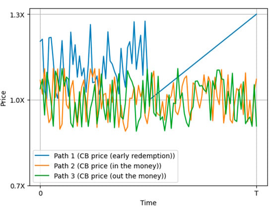Figure 1. Simulated Paths.

3.3. Foundations of Convertible Bond Valuation through Machine Learning Methodology

While commonplace in regression analysis, the ordinary least squares (OLS) method is subject to limitations such as overfitting and the misspecification of polynomial degrees of foundational functions and interactions between variables. Furthermore, performing OLS requires a sufficiently large data sample size, thus resulting in a considerable computational burden. To overcome limitations in linear regression within the Longstaff–Schwartz algorithm, some efforts have been spent on the improvement of the OLS under the LSM framework like matching projection pursuit, Gaussian process regression, and an enhanced GPR-MC framework. Details about approaches can be found in the work led by Tompaidis and Yang [40], Mu et al. [41], and Goudenège et al. [42]. Here, we also attempt to explore sensible alternatives to traditional linear regression. In this paper we follow the same framework of the basic LSM algorithm; only the continuation value is estimated by support vector regression or random forests instead of OLS.

3.3.1. Support Vector Regression

Unlike linear regression aiming to minimize the sum of squared errors, the objective function of support vector regression (SVR) is to find the minimum coefficients under the condition that the error term is set at an acceptable level. Therefore, using SVR in the model will give us more flexibility to control error to a certain degree and reduce the features used to avoid potential overfit.

The formulation of SVR is given by the following equations:

$$f\left(x,\beta \right)={\beta }^{t}x+c.$$

Define a specified margin $\epsilon$ that satisfies the equation:

$$|Z-f(x,\beta ){|}_{\epsilon }=\left\{\begin{array}{c}\begin{array}{c}0, if \left|Z-f\left(x,\beta \right)\right|\le \epsilon \\ \end{array}\\ \left|Z-f\left(x,\beta \right)\right|-\epsilon ,otherwise\end{array}\right..$$

The SVR aims to minimize the value of margin $\epsilon$ and the coefficient vector $\parallel \beta {\parallel }^2$ in Equation (2).

$$\begin{array}{c}R\left(f\right)=d{\displaystyle \sum _{i=1}^n} {\left|Z_i-f_i\left(x,\beta \right)\right|}_{\epsilon }+\frac{1}{2}\parallel \beta {\parallel }^2\end{array}$$

(2)

Equation (2) reduces to Equation (3) under the conditions defined in Equations (4) and (5).

$$\begin{array}{c}R\left(f\right)=d{\displaystyle \sum _{i=1}^n} \left({\zeta }_{\mathit{i}}+{\zeta }_i^{*}\right)+\frac{1}{2}\parallel \beta {\parallel }^2\end{array}$$

(3)

$$\begin{array}{c}\left({\beta }^t{x}_i+c\right)-Z_i\le \epsilon +{\zeta }_{\mathit{i}}\end{array}$$

(4)

$$\begin{array}{c}{Z}_i-\left({\beta }^t{x}_i+c\right)\le \epsilon +{\zeta }_i^{*}\end{array}$$

(5)

where ${\mathsf{\zeta }}_{\mathrm{i}}$ and ${\mathsf{\zeta }}_{\mathrm{i}}^{\mathrm{*}}$ are defined as slack variables to tolerate deviation from the margin $\epsilon$.

As an alternative to OLS in the LSM pricing model, we are allowed to decide how tolerant we are of errors by selecting an acceptable error margin and the tolerance value to deviate from the acceptable error rate. It is expected that SVR can attain a similarly satisfactory fitting result when the sample size is not sufficiently large.

Further, kernel functions can be used in SVR. The common forms of kernel functions include linear, radial basis function (RBF), and polynomial. In our empirical experiment, the radial basis function $K\left(x_i,x_j\right)=e^{\delta {∥x_i-x_j∥}^2}$ is chosen as the kernel and the hyperparameter $\delta >0$ is tuned to gain the desired accuracy of the model.

3.3.2. Random Forest

Breiman [43] introduced the random forest technique, an ensemble tree-based algorithm wherein a regression tree serves as the foundational regressor. In the classical least squares approach, the expected continuation values can be approximated by a linear regression on a countable set of basis functions of random variable $X$. In our study, a depth-p regression tree ${\mathcal{T}}_p\left(X\right)$ is used to estimate the continuation values. The basic idea is to write the conditional expectation of $X$ as a piecewise constant function of $X$.

Consider a partition $\mathcal{A}$ of $[0,1{]}^d$ with $2^p$ elements obtained in the regression tree ${\mathcal{T}}_p$.

For ${\left({\alpha }_p^n\right)}_{1\le n\le 2^p}\in {\mathbb{R}}^{2^p}$, ${\mathcal{P}}_p$ is defined as the piecewise constant function on the partition $\mathcal{A}$ with values ${\alpha }_p^n$. For $x\in [0,1{]}^d$,

$${\mathcal{P}}_p\left(x,{\left(a_p^{n-1}\right)}_{0\le n\le 2^p},{\left({\alpha }_p^n\right)}_{1\le n\le 2^p}\right)=\sum _{n=1}^{2^p} {\alpha }_p^n{\mathbb{1}}_{\left\{x\in \left[a_p^{n-1},a_p^n\right)\right\}}$$

If we choose ${\alpha }_p^n=\mathbb{E}\left[Y\mid X\in \left[a_p^{n-1},a_p^n\right)\right],$ then the regression tree ${\mathcal{T}}^p\left(X\right)$ can be written in this form:

$${\mathcal{T}}^p\left(X\right)={\mathcal{P}}_p\left(X,{\left(a_p^{n-1}\right)}_{0\le i\le 2^p},{\left({\alpha }_p^n\right)}_{1\le i\le 2^p}\right).$$

When exercised at time $t_i$, we denote the discounted payoff of the convertible bond:

$$Z_{t_j}=\sum _{j=i+1}^N \exp \left(-{\int }_{t_i}^{t_j} r(\omega ,s)ds\right)C(\omega ,t_j).$$

Then, the continuation value at a given time $t_i$ is

$$Y\left(\omega ;t_i\right)=E_{\mathrm{Q}}\left[Z_{t_j}\mid F_{t_i}\right].$$

${\tau }_i$ is the smallest optimal stopping time after $t_i$, that is,

$${\tau }_i=t_i{\mathbb{1}}_{\left\{{n_{t_i}S}_{t_i}\ge E_{\mathrm{Q}}\left[Z_{{\tau }_{i+1}\mid }\mid F_{t_i}\right]\right\}}+{\tau }_{i+1}{\mathbb{1}}_{\left\{{n_{t_i}S}_{t_i}<E_{\mathrm{Q}}\left[Z_{{\tau }_{i+1}}\mid F_{t_i}\right]\right\}}$$

The main task is to find the continuation value $E_{\mathrm{Q}}\left[Z_{{\tau }_{i+1}}\mid F_{t_i}\right]$ by the regression tree.

Let ${\left(\left[a_{n-1}\left(p\right),a_n\left(p\right)\right)\right)}_{1\le n\le 2^p}$ be the partition generated by ${\mathcal{T}}_i^p\left(S_{t_i}\right)$. We define

$${\mathcal{T}}_i^p\left(S_{t_i}\right)=\sum _{n=1}^{2^p} \mathbb{E}\left[Z_{{\tau }_{i+1}}\mid S_{t_i}\in \left[a_{n-1}\left(p\right),a_n\left(p\right)\right)\right]{\mathbb{1}}_{\left\{S_{t_i}\in \left[a_{n-1}\left(p\right),a_n\left(p\right)\right)\right\}}$$

Then, we use ${\mathcal{T}}_i^p\left(S_{t_i}\right)$ to approximate the continuation value $E_{\mathrm{Q}}\left[Z_{{\tau }_{i+1}}\mid F_{t_i}\right]$. The smallest optimal stopping time after $t_i$ is expressed as:

$${\tau }_i^p=t_i{\mathbb{1}}_{\left\{{n_{t_i}S}_{t_i}\ge {\tau }_i^p\left(S_{t_i}\right)\right\}}+{\tau }_{i+1}{\mathbb{1}}_{\left\{{n_{t_i}S}_{t_i}<{\tau }_i^p\left(S_{t_i}\right)\right\}}$$

The results for convergence of the expected continuation value have been given by the following theorem [44]:

Theorem 4.1.

$$\underset{p\to \mathrm{\infty }}{\mathrm{l}\mathrm{i}\mathrm{m}} \mathbb{E}\left[Z_{{\tau }_i^p}\mid {\mathcal{F}}_{t_i}\right]=\mathbb{E}\left[Z_{{\tau }_i}\mid {\mathcal{F}}_{t_i}\right] \mathrm{in} {\mathbb{L}}^2(\mathsf{\Omega }) \mathrm{for} 1\le i\le N$$

Next, we proceed to present the result for convergence of the LSM algorithm with regression trees. For the fixed regression tree depth $p$, we simulate $K$ stock price paths $S_{t_0}^{\left(k\right)},\dots ,S_{t_K}^{\left(k\right)}$ along with the corresponding payoff paths $Z_{t_0}^{\left(k\right)},\dots ,Z_{t_N}^{\left(k\right)},k=1,\dots ,K$. For each time point $t_i,$ $i=1,\dots ,N-1$ we approximate the conditional expectations $E_{\mathrm{Q}}\left[Z_{{\tau }_{i+1}}\mid F\left(\omega ;t_i\right)\right]$ on the path $k$ using the regression tree ${\widehat{\mathcal{T}}}_p^{i,K}\left(S_{t_i}^{\left(k\right)}\right)$. Finally, the present value of the convertible bond at $t_0$ is approximated by

$$V_{t_0}^{p,K}=\frac{1}{K}\sum _{k=1}^K Z_{{\widehat{\tau }}_i^{p,\left(k\right)}}^{\left(k\right)},$$

where ${\widehat{\tau }}_i^{p,\left(k\right)}=t_i{\mathbb{1}}_{\left\{Z_{t_i}^{\left(k\right)}\ge {\widehat{\mathcal{T}}}_p^{i,K}\left(X_{t_i}^{\left(k\right)}\right)\right\}}+{\widehat{\tau }}_{i+1}^{\left(k\right)}{\mathbb{1}}_{\left\{Z_{\mathrm{i}}^{\left(k\right)}<{\widehat{\mathcal{T}}}_p^{i,K}\left(X_{t_i}^{\left(k\right)}\right)\right\}}.$

It remains to show the convergent behavior of the estimated price as the number of sampled paths $K$ goes to infinity for a fixed depth. The convergence result is summarized in the following theorem.

Theorem 4.2.

Assume that for all $p\in {\mathbb{N}}^{*}$, and all $1\le i\le N-1,\mathbb{P}\left(Z_{t_i}={\mathcal{T}}_p^i\left(X_{t_i}\right)\right)=0$. Then, for $\alpha =\mathrm{1,2}$ and for every $i=1,\dots ,N$,

$$\underset{K\to \infty }{lim} \frac{1}{K}\sum _{k=1}^K {\left(Z_{{\tau }_i^{p,\left(k\right)}}^{\left(k\right)}\right)}^{\alpha }=\mathbb{E}\left[{\left(Z_{{\tau }_i^p}\right)}^{\alpha }\right] a.s.$$

The detailed proof can be seen in Ech-Chafiq et al. [44].

Note that Theorem 4.2 only proves the a.s. convergence of the estimated value for any fixed $p$ when $K$ goes to infinity. The limiting behavior is still not clear when both $K$ and $p$ go to infinity. In the empirical experiment, we will study the effect of increasing the number of simulated paths on pricing accuracy.

3.3.3. Bayesian Optimization

The computational time of the random forest method directly depends on the number of trees, the depth of the tree, and the number of samples in each node (leaf) inside the forest. The splitting strategy and input feature selection also affect the accuracy and robustness of the learning-based approach. Setting appropriate values for the parameters is crucial to cut down the computational cost to a manageable size and avoid the overfitting problem [45]. Bayesian optimization is a method of finding the minimum value of a function, which has been applied to the parameter value search in machine learning [46].

In this study, with the aid of Bayesian optimization, we select the values for the number of trees (n_estimators), the depth of the tree (max_depth), the maximum number of input features (max_features), the minimum number of samples of the split threshold (min_samples_split), and the minimum number of samples in each node (min_samples_leaf) as recorded in Table 3. Since the parameter value in the model must be an integer, the nearest integer value for each parameter is selected as the optimal value.

Table 3. Parameter Optimization Information.

Name	Value Range	Optimum Value (Simulation)	Optimum Value (Real Case)
max_depth	(5,20)	17.807	16.305
max_features	(0,20)	17	16
n_estimators	(10,150)	103.516	101.498
min_samples_split	(1,5)	3	2
min_samples_leaf	(1,5)	2	1

4. Empirical Studies

Our study uses numerical experiments to assess the effectiveness of our novel learning-based LSM algorithm. We start with simulated data analysis, adjusting simulation paths, and time increments for pricing accuracy. Then, we compare predicted prices for both methods with real-market valuations, focusing on the China Securities Convertible Bond as a key case study for pricing. Moreover, for the call option characteristics embedded in the convertible bond, we classified at-the-money (ATM) options as those with moneyness ranging from 0.95 to 1.05. In-the-money (ITM) options were defined as those with moneyness between 1.05 and 1.3, while out-of-the-money (OTM) options were identified as having moneyness values between 0.7 and 0.95. It is important to note that, in the context of convertible bond pricing, moneyness is determined by the ratio of the stock price to the conversion price.

4.1. Data Description

In China, banks typically dominate the convertible bond market in terms of the largest issuance volume, and convertible bonds issued by banks tend to carry higher credit ratings [34]. Therefore, our sample primarily chooses existing convertible bonds issued by China Everbright Bank (CEB) as of 1 January 2023. Descriptive statistics of the sample bond price are presented in Table 4, where we computed the maximum value, minimum value, median, standard deviation, mean, and three quartiles. The sample period ranges from 1 January 2022 to 31 December 2022 with price predicted every day as a time step. We utilized daily trading data of Everbright Bank’s convertible bonds, containing transaction prices, trading volumes, transaction dates, risk-free interest rates, and price volatility, among other factors. These real trading data reflect the market demand and trading behavior of investors in the convertible bond market. Our objective is to conduct pricing analysis to compare the accuracy of different models, namely, basic LSM with OLS, LSM with SVR, and LSM with RF. The deviation between predicted and observed values is measured by root mean square error (RMSE). As an indicator of model goodness-of-fit to check the degree of mispricing, RMSE indicates the average level of prediction error and is calculated as:

$$RSME=\sqrt{\frac{\sum {\left(y_i-{\widehat{y}}_i\right)}^2}{N-P}},$$

where $y_i$ is the actual value for the $i$th observation, ${\widehat{y}}_i$ is the predicted value for the $i$th observation, $N$ is the number of observations, $P$ is the number of parameter estimates.

Table 4. Descriptive statistics of sample data.

Name	Mean	Median	Max	Min
CEB	107.09	105.61	115.95	104.358
CB Price	STD	Q1	Q2	Q3
	2.18	105.04	105.61	106.82

4.2. Model Description

At first, a large number of stock price paths are generated through Monte Carlo simulation. For each path, three different regression techniques are used to estimate the value of continuation at each time step. The estimated continuation value is compared with the conversion value to determine whether immediate exercising is optimal. If immediate exercising is optimal based on the exercise rules, the exercise decision is revisited at the next exercise time step. This process iterates backward from the last time step until reaching the beginning. Finally, the mean of the exercise values across all paths is computed to derive the final price of the convertible, marking the conclusion of the algorithm.

Table 5 records the specific values for input parameters that are needed in the LSM pricing model. In the simulated data experiment, an initial stock price $S_0$ was set at 100 and for the real market data experiment, the closing stock price on the first day of the year 2022 was 112.97. The selection of volatility ${\sigma }_s$ refers to the long-term mean volatility of the underlying stock before the issuing date. As for the risk-free rate $r_0$, we choose the 6-year risk-free interest rate at the issuing date.

Table 5. Parameters of underlying assets of two studies.

	${\mathbf{S}}_0$	${\mathsf{\sigma }}_{\mathbf{s}}$	${\mathbf{r}}_0$
Simulated data	100.00	0.2672	0.03158
CEB	112.97	0.2672	0.03158

4.3. Simulated Data Study

Table 6 presents the results of various convertible bond pricing techniques, with initial stock price (${\mathrm{S}}_0$) set at 100, time to maturity (T) spanning from 1 month to 2 years, and conversion prices ranging from 70 to 130. The bond price obtained via the finite difference with a sufficiently large number of grids method serves as the benchmark for the comparison purpose. The root mean square error (RMSE) is computed as a metric for evaluating pricing accuracy from different models. A higher RMSE indicates a higher degree of mispricing and vice versa.

Table 6. RMSE results with 1000 simulated paths and 100 time steps.

Moneyness	Total	ITM	ATM	OTM
Bys-RF	0.4922	0.6001	0.6122	0.3673
SVR	0.5324	0.6326	0.6426	0.3987
LSM	0.7295	0.9355	0.8126	0.6532

Note: Bys-RF refers to the random forest model with hyperparameter tuning by Bayesian optimization and the parameter settings can be found in Table 2.

As presented in Table 6, both learning-based approaches achieve better results than the ordinary LSM model. Furthermore, the Bys-RF approach exhibits the best performance. As follows, we start to investigate the impact of the number of simulated paths and the number of time steps on the pricing accuracy. Detailed outcomes are displayed in Table 7 and Table 8.

Table 7. RMSE results for the different number of paths with 100 time steps.

Number of Paths	Moneyness	Bys-RF	SVR	LSM
500	Total	0.6345	0.6789	1.0224
	ITM	0.7536	0.7452	1.324
	ATM	0.6948	0.6879	1.0321
	OTM	0.4927	0.4523	0.7987
1000	Total	0.5011	0.5324	0.7295
	ITM	0.6012	0.6326	0.9355
	ATM	0.6023	0.6426	0.8126
	OTM	0.3751	0.3987	0.6532
1500	Total	0.4029	0.5221	0.6254
	ITM	0.5012	0.6178	0.7659
	ATM	0.4564	0.5748	0.6588
	OTM	0.2918	0.3889	0.5114

Table 8. RMSE results for the different numbers of time steps with 1000 simulated paths.

Number of Time Steps	Moneyness	Bys-RF	SVR	LSM
500	Total	0.5901	0.6144	0.6378
	ITM	0.6984	0.7865	0.8569
	ATM	0.6512	0.6978	0.7894
	OT	0.4325	0.4556	0.5985
1000	Total	0.4897	0.5324	0.7295
	ITM	0.6012	0.6326	0.9355
	ATM	0.6215	0.6426	0.8126
	OTM	0.3698	0.3987	0.6532
1500	Total	0.4215	0.5978	0.7015
	ITM	0.5078	0.7145	0.8123
	ATM	0.4598	0.6878	0.7564
	OTM	0.3021	0.4589	0.6545

From Table 7, it is evident that the price prediction error reduces along with the increasing number of simulation paths. Moreover, as the number of paths increases, the two learning-based models consistently yield more precise outcomes and the Bys-RF approach outperforms the other two algorithms given the same time steps. This particular outcome is consistent with Table 5, highlighting the advantage of the Bys-RF method used in LSM pricing analysis.

Table 8 reveals a similar result: under the impact of varying numbers of time steps, the Bys-RF model performs best among all different simulated scenarios. Interestingly, we can observe that only the pricing accuracy achieved by the Bys-RF model steadily improves with the increment in the number of time steps. The robust performance of the Bys-RF model validates the convergence results previously discussed.

4.4. A Case Study of CEB Convertible Bond

To test the real-world applicability of our proposed methods, we now perform a case study on the CEB convertible bond. There are two main reasons to select Everbright Bank’s convertible bonds for our research. Firstly, from an empirical perspective, Everbright Bank’s convertible bonds are a prominent and representative product, with significant issuance and trading activity that influences the Chinese financial market. Secondly, in terms of data availability, as a publicly listed company, Everbright Bank’s convertible bonds offer abundant and easily accessible data, including issuance announcements, financial reports, and market trading data. This rich dataset provides a robust foundation for our research, enhancing the reliability and validity of our empirical study. All of these make the CEB convertible bond an ideal subject for studying convertible bond pricing, exploring pricing mechanisms and investor behavior in the convertible bond market, and contributing to the research in finance and investment. Our study collected daily trading price data for this bond from 1 January 2022 to 1 December 2022 (see Table 9) and we simulated convertible bond pricing for the three models using 10,000 paths and 240 time steps (one year).

Table 9. CEB Convertible Bond Basic Terms.

Issue Date	2017.3.31
Time horizon	6
Face value	100
Coupon (%)	0.2, 0.5, 1.0, 1.5, 1.8, 2.0
Call value till maturity	105
The first conversion price	4.36
Change of conversion price	2017.7.5, adjusted to 4.26
Reset clause	In 30 consecutive trading days, the closing stock price is lower than 80% of the conversion price in 15 trading days
Call on condition	In 30 consecutive trading days, the closing stock price is not less than 130% of the conversion price in 15 trading days
Call value	Face value plus the accrued interest
Put on condition	When the use of the capital is changed
Put value	Face value plus the accrued interest
${\mathsf{\sigma }}_{\mathrm{s}}$	The long-term mean volatility of the underlying stock before the issuing date
r	The 6-year risk-free interest rate at the issuing date

Table 10 provides a summary of the performance of the three models. Similar to the results computed with simulated data, it is not surprising to see the RF model outperforms both SVR and LSM models. Nonetheless, the performance of the SVR method is not impressive as its prediction accuracy falls below that of the original LSM method. This observation also confirms our previous discussion that SVR might be more efficient when handling relatively small datasets, i.e., with fewer Monte Carlo pricing paths.

Table 10. RMSE results of CEB convertible bond valuation without tuning hyperparameters.

Moneyness	Total	ITM	ATM	OTM
RF	0.6589	0.7748	0.6897	0.5987
SVR	0.8945	1.0586	0.9465	0.7946
LSM	0.7365	1.0568	0.8654	0.7145

Note: RF represents the random forest model without hyperparameter tuning.

To explore the possibility of enhancing the model’s performance through the adjustment of hyperparameters, we conducted tests on China Everbright Bank (CEB) convertible bond data during the first quarter of the year 2022 by employing the Bayesian optimization method previously described for tuning the hyperparameters of the random forest (Table 2). Table 11 showcases the root mean square error (RMSE) for convertible bonds traded in the first quarter of the year 2022, allowing for a comparison with and without hyperparameter tuning.

Table 11. RMSE results with and without hyperparameter tuning.

	Moneyness	Bys-RF	SVR	LSM
With hyperparameter Tuning	Total	0.5233	0.7	0.7643
	ITM	0.5931	0.8235	0.8878
	ATM	0.5278	0.7978	0.8235
	OTM	0.4363	0.6912	0.6945
Without hyperparameter tuning	Total	0.6183	0.8141	0.7765
	ITM	0.7238	1.0186	0.9568
	ATM	0.6497	0.8451	0.8654
	OTM	0.5895	0.7546	0.7145

Both SVR and Bys-RF methods yield better results, as presented in Table 11. The performance of the Bys-RF method is superior to both SVR and LSM in both simulated data experiments and real market data experiments, irrespective of whether the hyperparameters were tuned or not.

In Figure 2, we compare the actual price and predicted price by using three models. It can be seen that the trend of both prices is roughly the same, and inflection points occur earlier than the real situation. The deviation of pricing results is mostly maintained within a very narrow range, illustrating that pricing results are excellent.

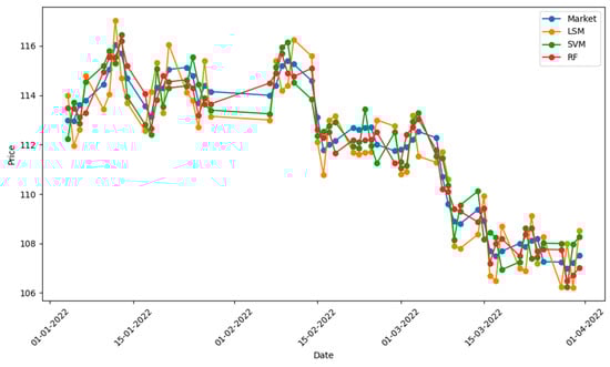
Figure 2. Market Price and Predicted Price for CEB Convertible Bonds.

In addition to examining error rates, we also measured the computational time of each model as shown in Table 12:

Table 12. Time Consumption Comparison.

Algorithm	Computational Cost Estimate	Estimated Computation Time	Reason for Difference
Traditional LSM	Moderate	About 10 min	Simple regression model fitting, relatively low computational complexity.
SVR replacing LSM	High	15–20 min	Support vector regression (SVR) involves solving a quadratic programming problem, which can be computationally intensive, especially for large datasets. It also requires tuning hyperparameters which may require additional computation.
RF replacing LSM	High	About 30 min	Random forest (RF) involves building multiple decision trees, each of which requires training on subsets of the data. For large datasets or a large number of trees, this can lead to significantly higher computational costs compared to simple regression. Additionally, tuning the RF hyperparameters adds to the computation time.
Bys-RF replacing LSM	Very high	30–40 min	Bayesian optimization iteratively explores the hyperparameter space of the random forest model to find optimal settings. While it can improve model performance, this iterative process requires additional computation, resulting in higher computational costs compared to standard random forest fitting.

As can be seen from the results in Table 12, the LSM model with Bys-RF produces the best result at the cost of the longest computation time. There may exist a tradeoff between pricing accuracy and computation cost. We concluded that for a comparable accuracy, a simpler algorithm like the basic LSM is efficient enough to deal with low-dimensional problems. However, for large datasets, it is interesting to consider using the improved LSM algorithm.

5. Conclusions and Limitations

In conclusion, our study proposes a novel approach for developing financial pricing models that integrate machine learning models. Specifically, we replace the OLS in the LSM model with two machine learning models, SVR and random forest, to construct a new model with improved pricing accuracy. Our simulation experiment demonstrates that the LSM model with SVR outperforms the traditional LSM model in terms of regression performance, particularly when the time step and simulated path quantity are increased.

Our study has significant implications for the financial industry, as integrating machine learning models into traditional pricing models can substantially enhance pricing accuracy. We suggest treading two new paths for future research: first, exploring the use of deep learning in LSM to further improve the accuracy of random forest and, second, applying the new model to more convertible bonds or investigating the usage of learning-based methods in clearly defining the links between valuation and the underlying risk factors.

Overall, our study contributes to the literature on financial pricing models by presenting a new approach that leverages machine learning models and by evaluating the performance of this approach through both simulation and market data experiments.

References

- Longstaff, F.; Schwartz, E. Valuing American options by simulation: A simple least-squares approach. Rev. Financ. Stud. 2001, 14, 113–147. [Google Scholar] [CrossRef]
- Luo, X.; Zhang, J. Pricing Chinese Convertible Bonds with Default Intensity by Monte Carlo Method. Discret. Dyn. Nat. Soc. 2019, 2019, 8610126. [Google Scholar] [CrossRef]
- Li, P.; Song, J. Pricing Chinese Convertible Bonds with Dynamic Credit Risk. Discret. Dyn. Nat. Soc. 2014, 2014, 492134. [Google Scholar] [CrossRef]
- Liu, J.; Yan, L.; Ma, C. Valuing Convertible Bonds Based on LSRQM Method. Discret. Dyn. Nat. Soc. 2014, 2014, 301282. [Google Scholar] [CrossRef]
- Nazemi, A.; Rauch, J.; Fabozzi, F.J. Interpretable Machine Learning for Creditor Recovery Rates. SSRN Electron. J. 2022. [Google Scholar] [CrossRef]
- Black, F.; Scholes, M. The Pricing of Options and Corporate Liabilities. J. Political Econ. 1973, 81, 637–654. [Google Scholar] [CrossRef]
- Merton, R.C. Theory of Rational Option Pricing. Bell J. Econ. Manag. Sci. 1973, 4, 141. [Google Scholar] [CrossRef]
- Merton, R.C. On the pricing of corporate debt: The risk structure of interest rates. J. Financ. 1974, 29, 449–470. [Google Scholar]
- Ingersoll, J.E. A contingent-claims valuation of convertible securities. J. Financ. Econ. 1977, 4, 289–321. [Google Scholar] [CrossRef]
- Brennan, M.J.; Schwartz, E.S. Convertible bonds: Valuation and optimal strategies for call and conversion. J. Financ. 1977, 32, 1699–1715. [Google Scholar] [CrossRef]
- Brennan, M.J.; Schwartz, E.S. Analyzing convertible bonds. J. Financ. Quant. Anal. 1980, 15, 907–929. [Google Scholar] [CrossRef]
- McConnell, J.J.; Schwartz, E.S. LYON taming. J. Financ. 1986, 41, 561–576. [Google Scholar] [CrossRef]
- Hull, J.; White, A. The Use of the Control Variate Technique in Option Pricing. J. Financ. Quant. Anal. 1988, 23, 237–251. [Google Scholar] [CrossRef]
- Kalotay, A.J.; Williams, G.O.; Fabozzi, F.J. A Model for Valuing Bonds and Embedded Options. Financ. Anal. J. 1993, 49, 35–46. [Google Scholar] [CrossRef]
- Duan, J.-C. The GARCH Option Pricing Model. Math. Financ. 1995, 1, 13–32. [Google Scholar] [CrossRef]
- Cox, J.C.; Ross, S.A.; Rubinstein, M. Option pricing: A simplified approach. J. Financ. Econ. 1979, 7, 229–263. [Google Scholar] [CrossRef]
- Hung, M.-W.; Wang, Y., Jr. Pricing Convertible Bonds Subject to Default Risk. Derivations 2002, 10, 75–87. [Google Scholar] [CrossRef]
- Das, S.R.; Sundaram, R.K. An Integrated Model for Hybrid Securities. Manag. Sci. 2007, 53, 1439–1451. [Google Scholar] [CrossRef][Green Version]
- Fu, M.C.; Laprise, S.B.; Madan, D.B.; Su, Y.; Wu, R. Pricing American options: A comparison of Monte Carlo simulation approaches. J. Comput. Financ. 2001, 4, 39–88. [Google Scholar] [CrossRef]
- Cortazar, G.; Gravet, M.; Urzua, J. The valuation of multidimensional American real options using the LSM simulation method. Comput. Oper. Res. 2008, 35, 113–129. [Google Scholar] [CrossRef]
- Nadarajah, S.; Margot, F.; Secomandi, N. Comparison of least squares Monte Carlo methods with applications to energy real options. Eur. J. Oper. Res. 2017, 256, 196–204. [Google Scholar] [CrossRef]
- Cecconi, F.; Khodabakhshian, A.; Rampini, L. Data-driven decision support system for building stocks energy retrofit policy. J. Build. Eng. 2022, 54, 104633. [Google Scholar] [CrossRef]
- Batten, J.A.; Khaw KL, H.; Young, M.R. Pricing convertible bonds. J. Bank. Financ. 2018, 92, 216–236. [Google Scholar] [CrossRef]
- Zheng, Z.; Lin, H. Research on the Pricing of Convertible Bonds in China. J. Xiamen Univ. (Philos. Soc. Sci. Ed.) 2004, 162, 93–99. [Google Scholar]
- Yang, J.; Choi, Y.; Li, S.; Yu, J. A note on “Monte Carlo analysis of convertible bonds with reset clause”. Eur. J. Oper. Res. 2010, 200, 924–925. [Google Scholar] [CrossRef]
- Feng, J.; Zhou, X.; Duan, M. Design and Impact Analysis of Convertible Bond Option Terms. Manag. Rev. 2018, 30, 58–68. [Google Scholar]
- Xie, Y. Research on Pricing of Convertible Bonds Based on Black-Scholes Model—Taking Oupai Convertible Bonds as an Example. China Price 2021, 11, 53–55. [Google Scholar]
- Yang, X.; Yu, J.; Xu, M.; Fan, W. Convertible bond pricing with partial integro-differential equation model. Math. Comput. Simul. 2018, 152, 35–50. [Google Scholar] [CrossRef]
- Chang, J.; Wang, Y. Pricing of Convertible Bonds Based on Tsallis Entropy Distribution under Stochastic Interest Rate Model. Oper. Res. Manag. 2020, 29, 189–197, 231. [Google Scholar]
- Takahashi, S.; Chen, Y.; Tanaka-Ishii, K. Modeling financial time-series with generative adversarial networks. Phys. A Stat. Mech. Appl. 2019, 527, 121261. [Google Scholar] [CrossRef]
- Dogariu, M.; Ştefan, L.-D.; Boteanu, B.A.; Lamba, C.; Ionescu, B. Towards Realistic Financial Time Series Generation via Generative Adversarial Learning. In Proceedings of the 29th European Signal Processing Conference (EUSIPCO), Dublin, Ireland, 23–27 August 2021. [Google Scholar]
- Zhou, W.; Yang, M.; Han, L. A Nonparametric Approach to Pricing Convertible Bond via Neural Network. In Proceedings of the Eighth ACIS International Conference on Software Engineering, Artificial Intelligence, Networking, and Parallel/Distributed Computing (SNPD 2007), Qingdao, China, 30 July–1 August 2007; Volume 2, pp. 564–569. [Google Scholar]
- Niu, X.; Ba, X. Pricing and Empirical Analysis of Convertible Bonds Based on Machine Learning. J. Party Sch. Guizhou Prov. 2021, 5, 58–71. [Google Scholar]
- Ren, G.; Meng, T. Research on Pricing Methods of Convertible Bonds Based on Deep Learning GAN Models. Int. J. Financ. Stud. 2024, 11, 145. [Google Scholar] [CrossRef]
- Fabozzi, F.J.; Paletta, T.; Tunaru, R. An improved least squares Monte Carlo valuation method based on heteroscedasticity. Eur. J. Oper. Res. 2017, 263, 698–706. [Google Scholar] [CrossRef]
- Jang, H.; Kim, S.; Han, J.; Lee, S.; Ban, J.; Han, H.; Lee, C.; Jeong, D.; Kim, J. Fast Monte Carlo Simulation for Pricing Equity-Linked Securities. Comput. Econ. 2019, 56, 865–882. [Google Scholar] [CrossRef]
- Andreasson, J.; Shevchenko, P.V. A bias-corrected Least-Squares Monte Carlo for solving multi-period utility models. Soc. Sci. Res. Netw. 2021. [Google Scholar] [CrossRef]
- Boire, F.M.; Reesor, R.M.; Stentoft, L. Bias Correction in the Least-Squares Monte Carlo Algorithm. SSRN Electron. J. 2022. [Google Scholar] [CrossRef]
- Lin, J.; Almeida, C. American option pricing with machine learning: An extension of the Longstaff-Schwartz method. Braz. Rev. Financ. 2021, 19, 85–109. [Google Scholar] [CrossRef]
- Tompaidis, S.; Yang, C. Pricing American-style options by Monte Carlo simulation: Alternatives to ordinary least squares. J. Comput. Financ. 2014, 18, 121–143. [Google Scholar] [CrossRef]
- Mu, G.; Godina, T.; Maffia, A.; Sun, Y.C. Supervised machine learning with control variates for American option pricing. Found. Comput. Decis. Sci. 2018, 43, 207–217. [Google Scholar] [CrossRef]
- Goudenège, L.; Molent, A.; Zanette, A. Machine learning for pricing American options in high-dimensional Markovian and non-Markovian models. Quant. Financ. 2020, 20, 573–591. [Google Scholar] [CrossRef]
- Breiman, L. Random Forests. Mach. Learn. 2001, 45, 5–32. [Google Scholar] [CrossRef]
- Ech-Chafiq, Z.E.F.; Labordère, P.H.; Lelong, J. Pricing Bermudan Options Using Regression Trees/Random Forests. SIAM J. Financ. Math. 2023, 14, 1113–1139. [Google Scholar] [CrossRef]
- Sun, D.; Wen, H.; Wang, D.; Xu, J. A random forest model of landslide susceptibility mapping based on hyperparameter optimization using Bayes algorithm. Geomorphology 2020, 362, 107201. [Google Scholar] [CrossRef]
- Guo, J.; Zan, X.; Wang, L.; Lei, L.; Ou, C.; Bai, S. A random forest regression with Bayesian optimization-based method for fatigue strength prediction of ferrous alloys. Eng. Fract. Mech. 2023, 293, 109714. [Google Scholar] [CrossRef]
Disclaimer/Publisher’s Note: The statements, opinions and data contained in all publications are solely those of the individual author(s) and contributor(s) and not of MDPI and/or the editor(s). MDPI and/or the editor(s) disclaim responsibility for any injury to people or property resulting from any ideas, methods, instructions or products referred to in the content. |
© 2024 by the authors. Licensee MDPI, Basel, Switzerland. This article is an open access article distributed under the terms and conditions of the Creative Commons Attribution (CC BY) license (https://creativecommons.org/licenses/by/4.0/).