Radial Basis Function–Finite Difference Solution Combined with Level-Set Embedded Boundary Method for Improving a Diffusive Logistic Model with a Free Boundary

Abstract

In this paper, we propose an efficient numerical method to solve the problems of diffusive logistic models with free boundaries, which are often used to simulate the spreading of new or invasive species. The boundary movement is tracked by the level-set method, where the Hamilton–Jacobi weighted essentially nonoscillatory (HJ-WENO) scheme is utilized to capture the boundary curve embedded by the Cartesian grids via the embedded boundary method. Then the radial basis function–finite difference (RBF-FD) method is adopted for spatial discretization and the implicit–explicit (IMEX) scheme is considered for time integration. A variety of numerical examples are utilized to demonstrate the evolution of the diffusive logistic model with different initial boundaries.

1. Introduction

Diffusive logistic models with free boundaries, commonly used to describe the spreading of new or invasive species in ecology, possess moving boundary problems. These moving boundary problems originate from physical and engineering problems [1,2] and, more recently, from decision and control theory and ecology [3]; the details can be found in Crank’s research [2]. The key characteristic of moving boundary problems is that the boundary of the domain is unknown but is determined by the governing equation. More precisely, the behavior of a moving boundary is strongly related to that of an unknown solution.

The first diffusive logistic model related to ecological invasion was established in 1937, without boundary constraints, and was independently proposed by Fisher [4] and Kolmogorov-Petrovsky-Piskunov (KPP) [5]. To the best of our knowledge, Du and Lin used the Stefan condition and solved the moving boundary problem of parabolic partial differential equations (PDEs) [3], which represented the first exploration in the field of population diffusion. In particular, the spreading–vanishing dichotomy of a one-dimensional case was demonstrated. The regularity and asymptotic behavior of the moving boundary $\partial \mathsf{\Omega }\left(t\right)$ and the solution $u(\mathbf{x},t)$ in high dimensions were studied in [6].

When numerically solving such a system, the main challenge arises from handling moving boundaries. To overcome this challenge and accurately measure both the inner and outer regions, the embedded boundary method [7,8] is commonly employed. This method involves embedding the complex geometry into a Cartesian mesh, which allows for the discretization of the intricate geometric regions. By incorporating the boundary into the computational domain, the embedded boundary method effectively addresses the difficulties associated with moving boundaries.

Moreover, to overcome the limitations of traditional grid-based methods, researchers have explored alternative approaches that offer greater flexibility and efficiency. One such approach is the use of radial basis functions (RBF) for multidimensional discrete data interpolation. In non-convex regions, where boundaries exhibit complex shapes and changes, radial basis function interpolation enables high adaptability for moving boundaries and irregular geometries, providing accurate interpolation results. Initially, RBF was used for global interpolation to solve PDEs by Kansa [9,10]. Global interpolation is easy to program and has spectral accuracy, but the resulting linear system is ill conditioned. In order to solve this shortcoming, local interpolation [11,12,13,14] methods are proposed. Among them, the radial basis function–finite difference (RBF-FD) method is popular. It is accurate, robust, computationally efficient, and geometrically flexible. Notably, the RBF-FD method stands out due to its ability to handle irregular and evolving domains. Unlike grid-based methods that require a structured mesh, the RBF-FD method operates on scattered nodes, allowing greater flexibility in representing complex geometries. In recent years, the RBF-FD method has been used to solve surface PDEs and has been applied to ecology, chemistry, geography, etc. [15,16,17].

The front-fixing method [18,19,20], the front-tracking method [18,19,21], and the level-set method [18,19,22,23,24] are three popular numerical methods of effectively dealing with moving boundaries. The front-fixing method is relatively simple and easy to implement compared to the other methods. However, its accuracy in simulating material interfaces with complex shape changes and internal structures may be limited. The front-tracking method is proposed to address the one-dimensional problem and the level-set method is proposed to handle the moving boundary for the two-dimensional problem by Liu et al. in [18,25]. Additionally, the front-tracking algorithm is also employed to solve a two-dimensional model with radial symmetry in [21]. The level-set method is generally robust in dealing with complex topological changes. When dealing with high-dimensional topological bifurcations, the level-set method enables greater efficacy in handling moving boundaries compared to the front-tracking method [19]. In practice, the level-set function is commonly used as the indicator function of the boundary when tracking its motion, and the corresponding boundary equation is typically solved using the Hamilton–Jacobi weighted essentially nonoscillatory (HJ-WENO) scheme [26].

The purpose of this paper is to solve the diffusive logistic model with moving boundaries. The embedded boundary method is employed to establish a fixed computational domain that distinguishes the interior and exterior regions. The interior of the domain is discretized using the radial basis function–finite difference method. Simultaneously, the boundary equation is solved using the HJ-WENO scheme, which determines the evolution of the moving boundary. In this paper, we determine the evolution of moving boundaries under different initial boundaries.

The rest of this paper is organized as follows. Section 2 presents a diffusive logistic model with a free boundary. In Section 3, the RBF-FD method is briefly reviewed, and the embedded boundary method for handling complex domains is presented. The numerical scheme for solving the diffusive logistic model with a stationary boundary is also given. The HJ-WENO scheme, which is used to solve the level-set equation, is introduced in Section 4. Additionally, the numerical algorithm for solving the diffusive logistic moving boundary problem is presented. Then, in Section 5, the convergence test for the embedded boundary method is demonstrated. Various numerical examples are performed to track the evolution of the moving boundary with different initial boundaries. Finally, we present our conclusion in Section 6. In addition, we give an appendix defining the abbreviations at the end of the article.

2. Problem Formulation

The diffusive logistic model has been widely used in simulations of the spreading of new or invasive species, with the free boundary representing the expanding front; it states that

$$\begin{array}{c}\hfill \frac{\partial u}{\partial t}-\gamma \Delta u=u(a-bu),t>0,\mathbf{x}\in \mathsf{\Omega }\left(t\right),\end{array}$$

(1)

subject to the boundary condition

$$\begin{array}{c}\hfill u(\mathbf{x},t)=0,t>0,\mathbf{x}\in \partial \mathsf{\Omega }\left(t\right),\end{array}$$

(2)

the Stefan condition

$$\begin{array}{c}\hfill {\rho }_t-\mu \nabla u·\nabla \rho =0,t>0,\mathbf{x}\in \mathsf{\Omega }\left(t\right),\end{array}$$

(3)

and the initial conditions

$$\begin{array}{c}\hfill \rho (\mathbf{x},0)={\rho }_0\left(\mathbf{x}\right),u(\mathbf{x},0)=u_0\left(\mathbf{x}\right),\mathbf{x}\in \mathsf{\Omega }\left(0\right),\end{array}$$

(4)

where $\mathsf{\Omega }$ represents the computational domain, $\Delta$ is the Laplacian operator, and ∇ is the gradient operator. $\gamma >0$ is the diffusive rate and $a>0$ and $b>0$ represent the intrinsic growth rate and the intraspecific competition, respectively. Here, $\partial \mathsf{\Omega }\left(t\right)$ represents the unknown moving boundary, $\rho$ denotes the level-set function, and $\mu >0$ denotes the proportionality constant between the species gradient at the front and the speed of the moving boundary. The initial function $u_0\left(\mathbf{x}\right)$ satisfies the following regularity condition:

$$\begin{array}{c}\hfill u_0\left(\mathbf{x}\right)\in C^2\left(\mathsf{\Omega }\left(0\right)\right),u_0\left(\mathbf{x}\right)>0,\mathbf{x}\in \mathsf{\Omega }\left(0\right).\end{array}$$

(5)

In the Stefan condition, $\rho$ represents the indicator function of the boundary as follows:

$$\rho (\mathbf{x},t)=\left\{\begin{array}{cc}\hfill +D,& \mathbf{x}\in \mathsf{\Omega }{\left(t\right)}^c,\hfill \\ \hfill 0,& \mathbf{x}\in \partial \mathsf{\Omega }\left(t\right),\hfill \\ \hfill -D,& \mathbf{x}\in \mathsf{\Omega }\left(t\right),\hfill \end{array}\right.$$

(6)

where D represents the Euclidean distance between the point $\mathbf{x}$ and the boundary $\partial \mathsf{\Omega }\left(t\right)$. $\mathsf{\Omega }{\left(t\right)}^c$ denotes the outside of the domain $\mathsf{\Omega }\left(t\right)$. The idea of introducing the level-set function is that the boundary is equal to the zero level set at any given time, i.e.,

$$\begin{array}{c}\hfill \partial \mathsf{\Omega }\left(t\right)=\left\{\mathbf{x}\right|\rho (\mathbf{x},t)=0\},\end{array}$$

(7)

where $\partial \mathsf{\Omega }\left(t\right)$ denotes the boundary of $\mathsf{\Omega }$ at time t.

3. Embedded Boundary Method with RBF-FD Discretization

In this part, we give a brief review on the RBF-FD discretization used for the given differential operator; then, the embedded boundary method is presented to address the complex domain, and an IMEX scheme is considered for the time integration of the diffusive logistic model with the stationary boundary.

3.1. RBF-FD Discretization

Given a differential operator $\mathcal{L}$, select the stencil ${\left\{{\mathbf{x}}_i\right\}}_{i=1}^n$ centered on point ${\mathbf{x}}_1$, where n is the stencil size; then, $\mathcal{L}u$ can be approximately expressed as a linear combination of the values of the functions at each stencil point, i.e.,

$$\begin{array}{c}\hfill {\mathcal{L}u\left(\mathbf{x}\right)|}_{\mathbf{x}={\mathbf{x}}_1}\approx \sum _{i=1}^n{w}_{i}u\left({\mathbf{x}}_i\right),\end{array}$$

(8)

where $w_1,w_2,\dots ,w_n$ are a set of weight coefficients.

Through the above stencil points ${\mathbf{x}}_1$, ${\mathbf{x}}_2$, …, ${\mathbf{x}}_n$ and with the function values $u\left({\mathbf{x}}_1\right)$, $u\left({\mathbf{x}}_2\right)$, …, $u\left({\mathbf{x}}_n\right)$ at the corresponding nodes, we use the following radial basis function coupled polynomial interpolation:

$$\begin{array}{c}\hfill u_h\left(\mathbf{x}\right)=\sum _{j=1}^n{c}_j\varphi (\parallel \mathbf{x}-{\mathbf{x}}_j\parallel )+\sum _{i=1}^m{\lambda }_i{P}_i\left(\mathbf{x}\right),\end{array}$$

(9)

subject to

$$\begin{array}{c}\hfill \sum _{j=1}^n{c}_j{P}_i\left({\mathbf{x}}_j\right)=0,i=1,2,\dots ,m,\end{array}$$

(10)

where $c_1,c_2,\dots ,c_n$ and ${\lambda }_1,{\lambda }_2,\dots ,{\lambda }_m$ are undetermined coefficients. $\varphi (\parallel \mathbf{x}-{\mathbf{x}}_j\parallel )$ is the radial basis function [27] and $\parallel ·\parallel$ represents the Euclidean distance. ${\left\{P_i\right\}}_{i=1}^m$ is the polynomial basis where m is the number of polynomial bases. The calculation formula of m is $m=\left(\genfrac{}{}{0pt}{}{p+d}{p}\right)$, p is the highest degree of the polynomial, and d is the space dimension. On the one hand, the addition of polynomial terms ensures that the radial function and polynomial space together form a complete space, preventing the matrix from being singular. On the other hand, this approach guarantees that the interpolation accuracy reaches at least polynomial accuracy.

Let ${\varphi }_j\left(\mathbf{x}\right)=\varphi (\parallel \mathbf{x}-{\mathbf{x}}_j\parallel )$ and $p=2$. The polynomial basis functions are given by $\{1,x,y,x^2,xy,y^2\}$. According to the interpolation condition $u_h\left({\mathbf{x}}_i\right){{|}_{i=1}^n=u\left({\mathbf{x}}_i\right)|}_{i=1}^n$, we can obtain a linear system:

$$\begin{array}{c}\hfill \left[\begin{array}{cccccccc}{\varphi }_1\left({\mathbf{x}}_1\right)& {\varphi }_2\left({\mathbf{x}}_1\right)& \cdots & {\varphi }_n\left({\mathbf{x}}_1\right)& 1& x_1& \cdots & y_1^2\\ {\varphi }_1\left({\mathbf{x}}_2\right)& {\varphi }_2\left({\mathbf{x}}_2\right)& \cdots & {\varphi }_n\left({\mathbf{x}}_2\right)& 1& x_2& \cdots & y_2^2\\ ⋮& ⋮& \ddots & ⋮& ⋮& ⋮& \ddots & ⋮\\ {\varphi }_1\left({\mathbf{x}}_n\right)& {\varphi }_2\left({\mathbf{x}}_n\right)& \cdots & {\varphi }_n\left({\mathbf{x}}_n\right)& 1& x_n& \cdots & y_n^2\\ 1& 1& \dots & 1& 0& 0& \dots & 0\\ x_1& x_2& \dots & x_n& 0& 0& \dots & 0\\ ⋮& ⋮& \ddots & ⋮& ⋮& ⋮& \ddots & ⋮\\ y_1^2& y_2^2& \dots & y_n^2& 0& 0& \dots & 0\end{array}\right]\left[\begin{array}{c}{c}_1\\ c_2\\ ⋮\\ c_n\\ {\lambda }_1\\ {\lambda }_2\\ ⋮\\ {\lambda }_m\end{array}\right]=\left[\begin{array}{c}u\left({\mathbf{x}}_1\right)\\ u\left({\mathbf{x}}_2\right)\\ ⋮\\ u\left({\mathbf{x}}_n\right)\\ 0\\ 0\\ ⋮\\ 0\end{array}\right],\end{array}$$

(11)

or equivalently, it can be written as the matrix form

$$\begin{array}{c}\hfill \left[\begin{array}{cc}A& P\\ P^T& 0\end{array}\right]\left[\begin{array}{c}\mathbf{c}\\ \lambda \end{array}\right]=\left[\begin{array}{c}\mathbf{u}\\ 0\end{array}\right],\end{array}$$

(12)

where $\mathbf{c}={(c_1,c_2,\dots ,c_n)}^T$, $\lambda ={({\lambda }_1,{\lambda }_2,\dots ,{\lambda }_m)}^T$, $\mathbf{u}={(u\left({\mathbf{x}}_1\right),u\left({\mathbf{x}}_2\right),\dots ,u\left({\mathbf{x}}_n\right))}^T$, A is the coefficient matrix of the radial basis function, and P is the coefficient matrix of the polynomial basis, which are defined as follows:

$$\begin{array}{c}\hfill A=\left[\begin{array}{cccc}{\varphi }_1\left({\mathbf{x}}_1\right)& {\varphi }_2\left({\mathbf{x}}_1\right)& \cdots & {\varphi }_n\left({\mathbf{x}}_1\right)\\ {\varphi }_1\left({\mathbf{x}}_2\right)& {\varphi }_2\left({\mathbf{x}}_2\right)& \cdots & {\varphi }_n\left({\mathbf{x}}_2\right)\\ ⋮& ⋮& \ddots & ⋮\\ {\varphi }_1\left({\mathbf{x}}_n\right)& {\varphi }_2\left({\mathbf{x}}_n\right)& \cdots & {\varphi }_n\left({\mathbf{x}}_n\right)\end{array}\right],P=\left[\begin{array}{cccc}1& x_1& \cdots & y_1^2\\ 1& x_2& \cdots & y_2^2\\ ⋮& ⋮& \ddots & ⋮\\ 1& x_n& \cdots & y_n^2\end{array}\right].\end{array}$$

It follows from the non-singularity of the interpolation matrix [17] that

$$\begin{array}{c}\hfill \left[\begin{array}{c}\mathbf{c}\\ \mathsf{\lambda }\end{array}\right]={\left[\begin{array}{cc}A& P\\ P^T& 0\end{array}\right]}^{-1}\left[\begin{array}{c}\mathbf{u}\\ 0\end{array}\right].\end{array}$$

(13)

Now, we apply the differential operator ${\mathcal{L}u\left(\mathbf{x}\right)|}_{\mathbf{x}={\mathbf{x}}_1}$ to the interpolation formula to obtain the differential relation:

$$\begin{array}{cc}\hfill {\mathcal{L}u\left(\mathbf{x}\right)|}_{\mathbf{x}={\mathbf{x}}_1}& \approx \mathcal{L}{u}_h{\left(\mathbf{x}\right)|}_{\mathbf{x}={\mathbf{x}}_1}\hfill \\ \hfill & =\sum _{j=1}^n{c}_j\mathcal{L}{\varphi }_j\left(\mathbf{x}\right){{|}_{\mathbf{x}={\mathbf{x}}_1}+\sum _{i=1}^m{\lambda }_i\mathcal{L}{P}_i\left(\mathbf{x}\right)|}_{\mathbf{x}={\mathbf{x}}_1}\hfill \\ \hfill & =\left[\begin{array}{cc}\mathcal{L}\varphi {\left(\mathbf{x}\right)}^T{|}_{\mathbf{x}={\mathbf{x}}_1}& \mathcal{L}P{\left(\mathbf{x}\right)}^T{|}_{\mathbf{x}={\mathbf{x}}_1}\end{array}\right]\left[\begin{array}{c}\mathbf{c}\\ \mathsf{\lambda }\end{array}\right]\hfill \\ \hfill & =\left[\begin{array}{cc}\mathcal{L}\varphi {\left(\mathbf{x}\right)}^T{|}_{\mathbf{x}={\mathbf{x}}_1}& \mathcal{L}P{\left(\mathbf{x}\right)}^T{|}_{\mathbf{x}={\mathbf{x}}_1}\end{array}\right]{\left[\begin{array}{cc}A& P\\ P^T& 0\end{array}\right]}^{-1}\left[\begin{array}{c}\mathbf{u}\\ 0\end{array}\right]\hfill \\ \hfill & =\left[\begin{array}{cc}{\mathbf{w}}^T& {\mathsf{\beta }}^T\end{array}\right]\left[\begin{array}{c}\mathbf{u}\\ 0\end{array}\right]={\mathbf{w}}^T\mathbf{u},\hfill \end{array}$$

(14)

where $\mathcal{L}\varphi \left(\mathbf{x}\right)={\left\{\mathcal{L}{\varphi }_j\left(\mathbf{x}\right)\right\}}_{j=1}^n$ and $\mathcal{L}P\left(\mathbf{x}\right)={\left\{\mathcal{L}{P}_i\left(\mathbf{x}\right)\right\}}_{i=1}^m$. The above equation can also deduce a weight formula:

$$\left[\begin{array}{cc}\mathcal{L}{\varphi }^T& \mathcal{L}{P}^T\end{array}\right]{\left[\begin{array}{cc}A& P\\ P^T& 0\end{array}\right]}^{-1}=\left[\begin{array}{cc}{\mathbf{w}}^T& {\mathsf{\beta }}^T\end{array}\right],$$

which, in turn, implies that

$$\left[\begin{array}{cc}A& P\\ P^T& 0\end{array}\right]\left[\begin{array}{c}\mathbf{w}\\ \mathsf{\beta }\end{array}\right]=\left[\begin{array}{c}\mathcal{L}\varphi \\ \mathcal{L}P\end{array}\right].$$

It is worth noting that the above computational process of weight coefficients only needs to retain $\mathbf{w}$. When the differential weights are obtained, we can discretize the differential operator by substituting it back to Equation (8).

Next, we will give the error estimates for the radial basis function interpolation [28].

Theorem 1.

Let Ω be a compact subset of ${\mathbb{R}}^d$ with a Lipschitz boundary. Let $1\le p,q\le \infty ,s\in \mathbb{R}$ with $s>d/p$ if $p>1$ or $s\ge d$ if $p=1$. Let $\mu \in \mathbb{N}$ satisfy $0\le \mu \le {}^{⌐}s-d{(1/p-1/q)}_{+}^{\neg }-1$. Also, let $X\subset \mathsf{\Omega }$ be a discrete set with mesh norm $h_{X,\mathsf{\Omega }}$. Then, there exists a constant depending only on Ω such that if $h_{X,\mathsf{\Omega }}\le h_0$ and if $u\in W_p^s\left(\mathsf{\Omega }\right)$, then

$$\parallel u-u_h{\parallel }_{W_q^{\mu }\left(\mathsf{\Omega }\right)}\le C{h}_{X,\mathsf{\Omega }}^{s-\mu -d{(\frac{1}{p}-\frac{1}{q})}_{+}}{\parallel u\parallel }_{W_p^s\left(\mathsf{\Omega }\right)},$$

(15)

where C is a positive constant independent of $h_{X,\mathsf{\Omega }}$, and ${\left(x\right)}_{+}=x$ if $x\ge 0$ and is 0 otherwise.

For $1\le p\le \infty$,

$$W_p^s\left(\mathsf{\Omega }\right)=\{u\in L^p\left(\mathsf{\Omega }\right)|D^{\alpha }u\in L^p\left(\mathsf{\Omega }\right),\left|\alpha \right|\le s\},$$

where $D^{\alpha }u$ represents the α-order weak derivative of u.

We define the norms as follows:

$$\begin{array}{c}\hfill \begin{array}{cc}\hfill {\parallel u\parallel }_{W_p^s\left(\mathsf{\Omega }\right)}& :={\left(\sum _{\left|\alpha \right|\le s}{\parallel D^{\alpha }u\parallel }_{L^p\left(\mathsf{\Omega }\right)}^p\right)}^{\frac{1}{p}},(1\le p<\infty ).\hfill \\ \hfill {\parallel u\parallel }_{W_{\infty }^s\left(\mathsf{\Omega }\right)}& :=\underset{\left|\alpha \right|\le s}{max}{\parallel D^{\alpha }u\parallel }_{L^{\infty }\left(\mathsf{\Omega }\right)},(p=\infty ).\hfill \end{array}\end{array}$$

(16)

Proof. 

The proof can be conducted in a similar way to the method in [29] [Corollary 13].    □

Remark 1.

Note that the RBF used in this paper is PHS-augmented with a quadratic polynomial; we immediately obtain

$$\begin{array}{cc}\hfill {∥u\left(\mathbf{x}\right)-u_h\left(\mathbf{x}\right)∥}_{L^{\infty }\left(\mathsf{\Omega }\right)}& \le C{h}_{X,\mathsf{\Omega }}^2{\parallel \Delta u\parallel }_{L^{\infty }\left(\mathsf{\Omega }\right)}=\mathcal{O}\left(h^2\right),\hfill \end{array}$$

(17)

$$\begin{array}{cc}\hfill {∥u\left(\mathbf{x}\right)-u_h\left(\mathbf{x}\right)∥}_{L^2\left(\mathsf{\Omega }\right)}& \le C{h}_{X,\mathsf{\Omega }}^2{\parallel \Delta u\parallel }_{L^2\left(\mathsf{\Omega }\right)}=\mathcal{O}\left(h^2\right).\hfill \end{array}$$

(18)

3.2. Embedded Boundary Method

The idea of the embedded boundary condition is to embed the complex geometry into the Cartesian mesh covering the entire computational domain. To this end, we recall the diffusive logistic model with the stationary boundary

$$\frac{\partial u}{\partial t}-\gamma \Delta u=u(a-bu),t>0,\mathbf{x}\in \mathsf{\Omega },$$

subject to the boundary condition

$$u(\mathbf{x},t)=0,t>0,\mathbf{x}\in \partial \mathsf{\Omega },$$

and the appropriate initial condition

$$u(\mathbf{x},0)=u_0\left(\mathbf{x}\right),\mathbf{x}\in \mathsf{\Omega }.$$

Assume $\mathsf{\Omega }$ is contained inside a rectangular domain $\tilde{\mathsf{\Omega }}=[0,L_1]\times [0,L_2],$ and for simplification, let $L_1=L_2=L$. Denote N as an integer, and let us discretize the spatial domain $\mathsf{\Omega }$ via a uniform mesh with the spatial step size $h=L/N$ as follows:

$$\begin{array}{c}\hfill {\tilde{\mathsf{\Omega }}}_h=\left\{(x_i,y_j)\right|x_i=ih,y_j=jh,0\le i,j\le N\}.\end{array}$$

(19)

Denote $T>0$ as the terminal time, and let $t_n=n\tau$, $0\le n\le T/\tau$, where $\tau$ is the time step size. Let $u_{i,j}^n=u_{i,j}\left(t_n\right)$ be the numerical approximation of u at the mesh point $(x_i,y_j)$ at time $t=t_n$.

Upon applying spatial discretization via the RBF-FD method as in the previous subsection for the Laplacian operator $\Delta$, denoted by ${\Delta }_h$, the corresponding space-discrete equation becomes an ordinary differential equation:

$$\frac{\partial u_h}{\partial t}-\gamma {\Delta }_h{u}_h=u_h(a-b{u}_h),$$

and then, an IMEX scheme is considered for time integration:

$$\begin{array}{c}\hfill \frac{u_h^{n+1}-u_h^n}{\tau }-\gamma {\Delta }_h{u}_h^{n+1}=u_h^n(a-b{u}_h^n).\end{array}$$

(20)

4. Level-Set Method with the HJ-WENO Scheme

A level-set function is utilized to capture the boundary movement. The governing equation determining the evolution of the boundary is given by

$$\left\{\begin{array}{ccc}\hfill & {\rho }_t-\mu \nabla u·\nabla \rho =0,\hfill & \hfill t>0,\mathbf{x}\in \tilde{\mathsf{\Omega }},\\ \hfill & \rho (\mathbf{x},0)={\rho }_0\left(\mathbf{x}\right),\hfill & \hfill \mathbf{x}\in \tilde{\mathsf{\Omega }},\end{array}\right.$$

(21)

where $\tilde{\mathsf{\Omega }}$ is the computational domain derived by the embedded boundary method. The level-set Equation (21) can be regarded as the special case of the Hamilton–Jacobi (HJ) equation, where $-\mu \nabla u·\nabla \rho$ is the Hamiltonian. Thus the HJ-WENO scheme can be used to discretize the level-set equation.

If we assume that $H({\rho }_x,{\rho }_y)=-\mu \nabla u·\nabla \rho =-\mu u_x{\rho }_x-\mu u_y{\rho }_y$, the level-set equation can be discretized in the following form [26]:

$$\begin{array}{c}\hfill \begin{array}{cc}\hfill \frac{d{\rho }_{i,j}}{dt}& =-\widehat{H}({\rho }_{x,i,j}^{+},{\rho }_{x,i,j}^{-},{\rho }_{y,i,j}^{+},{\rho }_{y,i,j}^{-}),\hfill \end{array}\end{array}$$

(22)

where ${\rho }_{x,i,j}^{-}$ and ${\rho }_{x,i,j}^{+}$ are the approximate values of ${\rho }_x(x_i,y_j)$ obtained on the left and right stencils illustrated in Figure 1, respectively. ${\rho }_{y,i,j}^{+}$ and ${\rho }_{y,i,j}^{-}$ are similar. $\widehat{H}$ is a Lipschitz continuous monotone flux, which is consistent with the Hamiltonian H, i.e., $\widehat{H}({\rho }_x^{+},{\rho }_x^{-},{\rho }_y^{+},{\rho }_y^{-})=H({\rho }_x,{\rho }_y)$. In this paper, we use the Lax–Friedrichs (LF) flux:

$$\begin{array}{c}\hfill \widehat{H}({\rho }_x^{+},{\rho }_x^{-},{\rho }_y^{+},{\rho }_y^{-})=H(\frac{{\rho }_x^{+}+{\rho }_x^{-}}{2},\frac{{\rho }_y^{+}+{\rho }_y^{-}}{2})-\alpha ({\rho }_x^{+},{\rho }_x^{-})\frac{{\rho }_x^{+}-{\rho }_x^{-}}{2}-\beta ({\rho }_y^{+},{\rho }_y^{-})\frac{{\rho }_y^{+}-{\rho }_y^{-}}{2}\end{array}$$

with

$$\alpha ({\rho }_x^{+},{\rho }_x^{-})=\underset{{\rho }_x\in I({\rho }_x^{-},{\rho }_x^{+})}{max}|H^{\prime }\left({\rho }_x\right)|=\mu \underset{\mathbf{x}\in \tilde{\mathsf{\Omega }}}{max}\left|u_x\right|,$$

$$\beta ({\rho }_y^{+},{\rho }_y^{-})=\underset{{\rho }_y\in I({\rho }_y^{-},{\rho }_y^{+})}{max}|H^{\prime }\left({\rho }_y\right)|=\mu \underset{\mathbf{x}\in \tilde{\mathsf{\Omega }}}{max}\left|u_y\right|,$$

where $I(a,b)=[min(a,b),max(a,b\left)\right].$

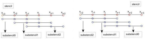
Figure 1. The left-biased stencil and the right-biased stencil.

In the same way, we also obtain the approximate value $u_{x,i,j}^{+},u_{x,i,j}^{-},u_{y,i,j}^{+},u_{y,i,j}^{-}$ of $u_x(x_i,y_j)$ and $u_y(x_i,y_j)$ using the fifth-order HJ-WENO reconstruction. Then, we obtain

$$\begin{array}{c}\hfill u_{x,i,j}=\omega u_{x,i,j}^{+}+(1-\omega )u_{x,i,j}^{-},\end{array}$$

(23)

where $\omega \in [0,1]$ is the weight coefficient. Similarly, $u_{y,i,j}$ can be obtained. After the overall reconstruction, we adapt the TVD scheme to the semi-discrete system:

$$\begin{array}{c}\hfill \begin{array}{cc}\hfill \frac{{\rho }_{i,j}^{n+1}-{\rho }_{i,j}^n}{\tau }=& \mu u_{x,i,j}^n\frac{{\rho }_{x,i,j}^{n,+}+{\rho }_{x,i,j}^{n,-}}{2}+\mu u_{y,i,j}^n\frac{{\rho }_{y,i,j}^{n,+}+{\rho }_{y,i,j}^{n,-}}{2}\hfill \\ \hfill & +\alpha ({\rho }_{x,i,j}^{n,+},{\rho }_{x,i,j}^{n,-})\frac{{\rho }_{x,i,j}^{n,+}-{\rho }_{x,i,j}^{n,-}}{2}+\beta ({\rho }_{y,i,j}^{n,+},{\rho }_{y,i,j}^{n,-})\frac{{\rho }_{y,i,j}^{n,+}-{\rho }_{y,i,j}^{n,-}}{2}\hfill \\ \hfill :=& L({\rho }_{i,j}^n,u_{i,j}^n).\hfill \end{array}\end{array}$$

(24)

For the moving boundary problem described in Equation (1), it is challenging to solve the diffusive logistic model accurately and effectively due to the evolving computational boundary over time. We couple the embedded boundary method and level-set method to develop an efficient numerical scheme. The details are as follows (Algorithm 1):

Algorithm 1

Step 1: Set a sufficient large rectangular domain $\tilde{\mathsf{\Omega }}\subset R^2$, so that the whole irregular area $\mathsf{\Omega }\left(t\right)\subset \tilde{\mathsf{\Omega }}$ for $t\in [0,T]$. Initialize the level-set function ${\rho }^0$ and $u^0$. Set $n=0$. Step 2: Solve (20) over $\tilde{\mathsf{\Omega }}$ to obtain $u^{n+1}$. Step 3: Solve (24) over $\tilde{\mathsf{\Omega }}$ to obtain ${\rho }^{n+1}$. Step 4: Set $n:=n+1$. Steps 1 and 2 are repeated over time until the final simulation time is reached.

5. Numerical Experiments

In this part, we perform the simulation of the evolution process of the moving boundary in various regions. The polyharmonic spline (PHS) radial basis function with $\varphi \left(r\right)=r^5$ augmented with the quadratic polynomial is adopted for RBF-FD spatial discretization, which does not need to determine the shape parameters and thus simplifies the calculation compared with the other parameter-determined radial basis functions (see [30]). And the closest point method is utilized to select the stencil point where the number of stencil points is 13 around the central node. The embedded computational domain is always set to ${[-1,1]}^2$ in two-dimensional space.

5.1. Convergence Test for Embedded Boundary Method

In this example, we consider the Poisson equation $\nabla ·\left(c\right(x,y)\nabla u)=f(x,y)$ in an irregular domain $\mathsf{\Omega }$, which is determined by the parameterized boundary interface:

$$\left\{\begin{array}{c}\hfill \begin{array}{cc}& \rho =r-(0.5+0.2sin(5\theta \left)\right),\hfill \\ & \theta =arctan(y/x),\hfill \\ & r=\sqrt{x^2+y^2},\hfill \end{array}\end{array}\right.$$

with the exact solution $u=e^x+e^y$. The diffusion coefficient $c(x,y)=2+sin\left(xy\right)$, and the forcing term $f(x,y)$ is computed using the exact solution.

The convergence results of the solution for the two-dimensional variable coefficient Poisson equation are shown in Table 1, which reports the spatial error in the $L^2$ norm and $L^{\infty }$ norm and the corresponding convergence rate. The numerical solution and the numerical error with $N=1280$ are presented in Figure 2. It can be observed that the spatial convergence rate of the embedded boundary method is of second order, which is consistent with the theoretical prediction in Theorem 1.

Table 1. Spatial error in $L^2$ norm and $L^{\infty }$ norm and corresponding convergence rate.

N	${\mathit{L}}^2$ Error	Rate	${\mathit{L}}^{\mathit{\infty }}$ Error	Rate
40	6.0670 × 10−6	-	1.3948 × 10−5	-
80	1.4202 × 10−6	$2.09$	3.3572 × 10−6	$2.05$
160	3.4323 × 10−7	$2.05$	8.2027 × 10−7	$2.03$
320	8.3416 × 10−8	$2.04$	2.0084 × 10−7	$2.03$
640	2.0532 × 10−8	$2.02$	4.9634 × 10−8	$2.02$
1280	5.1003 × 10−9	$2.01$	1.2351 × 10−8	$2.01$

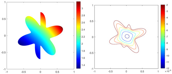
Figure 2. Profiles of numerical solution (left) and error (right) in the irregular domain with $N=1280$.

5.2. Numerical Tests for Diffusive Logistic Model with a Free Boundary

In this part, we next consider the diffusive logistic model (1) with the different parameter settings with the specific initial value and initial level-set function. The time–space step size is always set at $\tau =1e-4$ and $h=1/40$. The terminal time is $T=0.1$.

Example 1.

The initial boundary is set as a circle, where the center of the circle is at the origin point $(0,0)$, and the radius is $0.5$, with the initial level-set function given by

$$\begin{array}{c}\hfill \rho (x,y,0)=-(0.5-\sqrt{x^2+y^2}).\end{array}$$

(25)

The initial value is $u(x,y,0)=5cos\left(\sqrt{x^2+y^2}\pi \right)$. The parameter settings are set at $(\gamma ,\mu ,a,b)=(1,1,1,1)$.

Figure 3 shows the evolutions of the numerical solution and the moving boundary at t = 0.0002, 0.0242, 0.0661, and 0.1, respectively. It can be seen that the circle propagates in the form of a circle and the circular area becomes larger and larger as time progresses, which is in agreement with the results of [6]. The calculation time is 259.625.

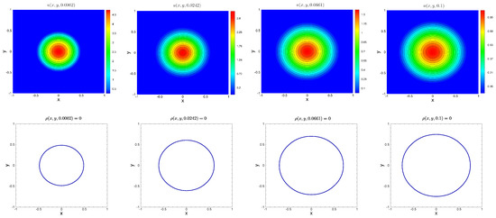
Figure 3. The evolutions of the numerical solution $u(x,y,t)$ and the moving boundary when the initial boundary is circular.

Example 2.

The initial boundary is set as an equilateral triangle centered at the origin point $(0,0)$ with a side length of 1, with the initial level-set function defined by

$$\begin{array}{c}\hfill \begin{array}{cc}\hfill & \rho (x,y,0)=-min(\frac{\sqrt{3}}{2}-\frac{1}{\sqrt{3}}+y,\sqrt{3}x-y+\frac{1}{\sqrt{3}},-\sqrt{3}x-y+\frac{1}{\sqrt{3}}).\hfill \end{array}\end{array}$$

(26)

The initial value is $u(x,y,0)=10(\frac{\sqrt{3}}{2}-\frac{1}{\sqrt{3}}+y)(\sqrt{3}x-y+\frac{1}{\sqrt{3}})(-\sqrt{3}x-y+\frac{1}{\sqrt{3}})$. The parameter settings are $(\gamma ,\mu ,a,b)$ = $(1,10,1,1)$.

Example 3.

The initial boundary is set as a square where the center of the square is at the origin point $(0,0)$, and the side length is 0.6, with the initial level-set function expressed as

$$\begin{array}{c}\hfill \begin{array}{c}\hfill \rho (x,y,0)=-min(0.3-|x|,0.3-|y\left|\right).\end{array}\end{array}$$

(27)

The initial value is $u(x,y,0)=100(0.3^2-x^2)(0.3^2-y^2)$. The parameter settings are set at $(\gamma ,\mu ,a,b)$ = $(1,10,1,1)$.

Figure 4 shows the evolutions of the numerical solution and the moving boundary at t = 0.0015, 0.0357, 0.0812, and 0.1, respectively. It can be observed that the initial square boundary eventually evolves into a circle and propagates in the form of a circle, which is consistent with that in [6]. The calculation time is 479.734.

Figure 4. The evolutions of the numerical solution $u(x,y,t)$ and the moving boundary when the initial boundary is a square.

Figure 5 shows the evolutions of the numerical solution and the moving boundary at t = 0.0001, 0.0094, 0.0301, and 0.1, respectively, from which it can be observed that the moving boundary asymptotically evolves into a circle, which is consistent with the asymptotic behavior described in [6]. The calculation time is 322.750.

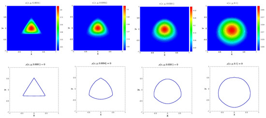
Figure 5. The evolutions of the numerical solution $u(x,y,t)$ and the moving boundary when the initial boundary is a triangle.

Example 4.

The initial boundary is set as a rectangle with the two adjacent sides measuring 0.6 and 0.8 respectively, with the initial level-set function

$$\begin{array}{c}\hfill \begin{array}{cc}\hfill & \rho (x,y,0)=-min(0.3-|x|,0.4-|y\left|\right).\hfill \end{array}\end{array}$$

(28)

The initial value is $u(x,y,0)=100(0.3^2-x^2)(0.4^2-y^2)$. The parameter settings are $(\gamma ,\mu ,a,b)$ = $(1,10,1,1)$.

Figure 6 depicts the evolutions of the numerical solution and the moving boundary at t = 0.0002, 0.0311, 0.0702, and 0.1, respectively, from which we can see that the boundary evolves into a circle and propagates gradually over time, which is in accordance with the prediction made in [6]. The calculation time is 259.625.

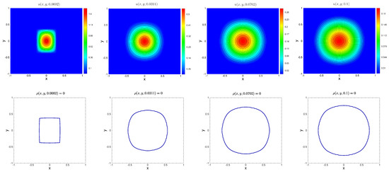
Figure 6. The evolutions of the numerical solution $u(x,y,t)$ and the moving boundary when the initial boundary is a rectangle.

The above numerical examples are carried out at $T=0.1$. In order to observe the boundary evolution over a longer period, we take the circular region as an example:

In the Figure 7, we choose T = 0.1, 1, 2. Obviously, the circular region becomes larger, and u tends to 0.

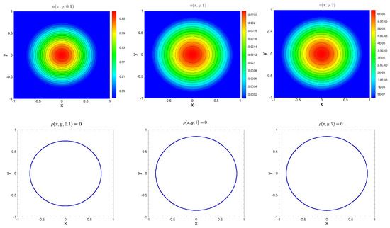
Figure 7. The evolutions of the numerical solution $u(x,y,t)$ and the moving boundary when the initial boundary is circular over a longer period.

6. Conclusions

In this paper, we incorporated the embedded boundary method with RBF-FD discretization and the level-set method with the HJ-WENO scheme to systematically investigate a diffusive logistic model with a free boundary. The embedded boundary method embeds the moving boundary within a rectangular domain to facilitate the construction of the discrete scheme, in which spatial discretization is achieved by the RBF-FD method. Additionally, the HJ-WENO scheme is employed to discretize the level-set convection equation, and thus, the moving boundary is obtained. Various numerical experiments are conducted to demonstrate the capability and efficiency of the proposed scheme in treating the irregular geometry. Moreover, we can observe that moving boundaries with initial regions shaped as circles, squares, triangles, and rectangles undergo changes and asymptotically evolve into circular shapes over time. Determining how to extend to more complex diffusive models with a free boundary will be the focus of our future research. Specifically, a more component diffusive logistic model with a free boundary will be studied later.

References

- Duffy, D.J. Finite Difference Methods in Financial Engineering: A Partial Differential Equation Approach; John Wiley & Sons: Hoboken, NJ, USA, 2013. [Google Scholar]
- Tayler, A.B. Free and moving boundary problems. J. Fluid Mech. 1985, 158, 532–533. [Google Scholar] [CrossRef]
- Du, Y.; Lin, Z. Spreading-vanishing dichotomy in the diffusive logistic model with a free boundary. SIAM J. Math. Anal. 2010, 42, 377–405. [Google Scholar] [CrossRef]
- Fisher, R.A. The wave of advance of advantageous genes. Ann. Eugen. 1937, 7, 355–369. [Google Scholar] [CrossRef]
- Kolmogorov, A. Étude de l’ équation de la diffusion avec croissance de la quantité de matière et son application à un problème biologigue. Moscow Univ. Bull. Ser. Internat. Sect. A 1937, 1, 1. [Google Scholar]
- Du, Y.; Matano, H.; Wang, K. Regularity and asymptotic behavior of nonlinear Stefan problems. Arch. Ration. Mech. An. 2014, 212, 957–1010. [Google Scholar] [CrossRef]
- Johansen, H.; Colella, P.A. Cartesian grid embedded boundary method for Poisson’s equation on irregular domains. J. Comput. Phys. 1998, 147, 60–85. [Google Scholar] [CrossRef]
- Peng, Z.; Appelö, D.; Liu, S. Universal AMG accelerated embedded boundary method without small cell stiffness. J. Sci. Comput. 2023, 97, 1–29. [Google Scholar] [CrossRef]
- Kansa, E.J. Multiquadrics-A scattered data approximation scheme with applications to computational fluid-dynamics-I surface approximations and partial derivative estimates. Comput. Math. Appl. 1990, 19, 127–145. [Google Scholar] [CrossRef]
- Kansa, E.J. Multiquadrics-A scattered data approximation scheme with applications to computational fluid-dynamics-II solutions to parabolic, hyperbolic and elliptic partial differential equations. Comput. Math. Appl. 1990, 19, 147–161. [Google Scholar] [CrossRef]
- Bayona, V.; Moscoso, M.; Carretero, M.; Kindelan, M. RBF-FD formulas and convergence properties. J. Comput. Phys. 2010, 229, 8281–8295. [Google Scholar] [CrossRef]
- Bayona, V.; Moscoso, M.; Kindelan, M. Optimal constant shape parameter for multiquadric based RBF-FD method. J. Comput. Phys. 2011, 230, 7384–7399. [Google Scholar] [CrossRef]
- Cecil, T.; Qian, J.; Osher, S. Numerical methods for high dimensional Hamilton-Jacobi equations using radial basis functions. J. Comput. Phys. 2004, 196, 327–347. [Google Scholar] [CrossRef]
- Fornberg, B.; Flyer, N. Solving PDEs with radial basis functions. Acta Numer. 2015, 24, 215–258. [Google Scholar] [CrossRef]
- Álvarez, D.; González-Rodríguez, P.; Kindelan, M. A local radial basis function method for the Laplace-Beltrami operator. J. Sci. Comput. 2021, 86, 28. [Google Scholar]
- Flyer, N.; Fornberg, B.; Bayona, V.; Barnett, G.A. On the role of polynomials in RBF-FD approximations: I. Interpolation and accuracy. J. Comput. Phys. 2016, 321, 21–38. [Google Scholar] [CrossRef]
- Shaw, S.B. Radial Basis Function Finite Difference Approximations of the Laplace-Beltrami Operator. Master’s Thesis, Boise State University, Boise, ID, USA, 2019. [Google Scholar]
- Liu, S.; Liu, X. Numerical methods for a two-species competition-diffusion model with free boundaries. Mathematics 2018, 6, 72. [Google Scholar] [CrossRef]
- Liu, S. Numerical Methods for A Class of Reaction-Diffusion Equations with Free Boundaries. Ph.D. Thesis, University of South Carolina, Columbia, SC, USA, 2019. [Google Scholar]
- Piqueras, M.A.; Company, R.; Jódar, L. A front-fixing numerical method for a free boundary nonlinear diffusion logistic population model. J. Comput. Appl. Math. 2017, 309, 473–481. [Google Scholar] [CrossRef]
- Liu, S.; Du, Y.; Liu, X. Numerical studies of a class of reaction-diffusion equations with Stefan conditions. Int. J. Comput. Math. 2020, 97, 9597–9979. [Google Scholar] [CrossRef]
- Chen, S.; Merriman, B.; Osher, S.; Smereka, P. A simple level set method for solving Stefan problems. J. Comput. Phys. 1997, 135, 8–29. [Google Scholar] [CrossRef]
- Osher, S.; Fedkiw, R.P. Level set methods: An overview and some recent results. J. Comput. Phys. 2001, 169, 463–502. [Google Scholar] [CrossRef]
- Osher, S.; Sethian, J.A. Fronts propagating with curvature-dependent speed: Algorithms based on Hamilton-Jacobi formulations. J. Comput. Phys. 1988, 79, 12–49. [Google Scholar] [CrossRef]
- Liu, S.; Liu, X. Exponential Time Differencing Method for a Reaction-Diffusion System with Free Boundary. Com. Appl. Math. Comput. 2023, 6, 354–371. [Google Scholar] [CrossRef]
- Jiang, G.S.; Peng, D. Weighted ENO schemes for Hamilton-Jacobi equations. SIAM J. Sci. Comput. 2000, 21, 2126–2143. [Google Scholar] [CrossRef]
- Liu, Y.; Qiao, Y.; Feng, X. A stable radial basis function partition of unity method for solving convection-diffusion equations on surfaces. Eng. Anal. Bound. Elem. 2023, 155, 148–159. [Google Scholar] [CrossRef]
- Johnson, M.J. An error analysis for radial basis function interpolation. Numer. Math. 2004, 98, 675–694. [Google Scholar] [CrossRef][Green Version]
- Fuselier, E.; Wright, G.B. Scattered data interpolation on embedded submanifolds with restricted positive definite kernels: Sobolev error estimates. SIAM J. Numer. Anal. 2012, 50, 1753–1776. [Google Scholar] [CrossRef]
- Barnett, G.A. A Robust RBF-FD Formulation Based on Polyharmonic Splines and Polynomials. Ph.D. Thesis, University of Colorado Boulder, Boulder, CO, USA, 2015. [Google Scholar]
Disclaimer/Publisher’s Note: The statements, opinions and data contained in all publications are solely those of the individual author(s) and contributor(s) and not of MDPI and/or the editor(s). MDPI and/or the editor(s) disclaim responsibility for any injury to people or property resulting from any ideas, methods, instructions or products referred to in the content. |
© 2024 by the authors. Licensee MDPI, Basel, Switzerland. This article is an open access article distributed under the terms and conditions of the Creative Commons Attribution (CC BY) license (https://creativecommons.org/licenses/by/4.0/).