Skew-Symmetric Generalized Normal and Generalized t Distributions

Abstract

In this paper, we introduce the skew-symmetric generalized normal and the skew-symmetric generalized t distributions, which are skewed extensions of symmetric special cases of generalized skew-normal and generalized skew-t distributions, respectively. We derive key distributional properties for these new distributions, including a recurrence relation and an explicit form for the cumulative distribution function (cdf) of the skew-symmetric generalized t distribution. Numerical examples including a simulation study and a real data analysis are presented to illustrate the practical applicability of these distributions.

1. Introduction

Azzalini [1] introduced the skew-normal distribution $SN\left(\lambda \right)$ characterized by the following density function:

$$2\varphi \left(x\right)\Phi \left(\lambda x\right),x\in \mathbb{R},$$

where $\varphi (·)$ represents the normal density function, and $\Phi (·)$ denotes the standard normal cumulative distribution function. The $SN$ distribution has gained considerable attention due to its ability to capture asymmetry in data while preserving key characteristics of the normal distribution. Its flexibility has made it particularly useful in various fields, such as finance, environmental studies, and biomedical research.

Subsequently, Jamalizadeh et al. [2] proposed a two-parameter generalized SN distribution $GSN({\lambda }_1,{\lambda }_2)$ with the following density function:

$${\varphi }_{GSN}(x;{\lambda }_1,{\lambda }_2)={\displaystyle \frac{2\pi }{{cos}^{-1}\left(\frac{-{\lambda }_1{\lambda }_2}{\sqrt{1+{\lambda }_1^2}\sqrt{1+{\lambda }_2^2}}\right)}}\varphi \left(x\right)\Phi \left({\lambda }_{1}x\right)\Phi \left({\lambda }_{2}x\right),x\in \mathbb{R},$$

where ${\lambda }_1$ and ${\lambda }_2$ are real numbers that enhance the model’s flexibility in capturing asymmetric data distributions. This two-parameter model effectively accommodates a wider range of skewness and kurtosis, offering more flexibility compared to its one-parameter counterpart.

Building on this, Jamalizadeh and Balakrishnan [3] introduced a three-parameter $GSN$ distribution $GSN({\lambda }_1,{\lambda }_2,\rho )$, which can be viewed as a special case of the unified multivariate skew-normal distribution introduced by Arellano-Valle and Azzalini [4]. The density function of $GSN$ is defined as follows:

$${\varphi }_{GSN}(x;{\lambda }_1,{\lambda }_2,\rho )={\displaystyle \frac{2\pi }{{cos}^{-1}\left(\frac{-(\rho +{\lambda }_1{\lambda }_2)}{\sqrt{1+{\lambda }_1^2}\sqrt{1+{\lambda }_2^2}}\right)}}\varphi \left(x\right){\Phi }_2({\lambda }_{1}x,{\lambda }_{2}x,\rho ),x\in \mathbb{R},$$

(1)

where ${\Phi }_2$ represents the cumulative distribution function of the standard bivariate normal distribution with correlation $\rho$ (with $\left|\rho \right|<1$). This three-parameter model enhances the distribution’s capability to provide a more flexible fit for complex datasets and to accommodate dependencies between variables.

Remark 1.

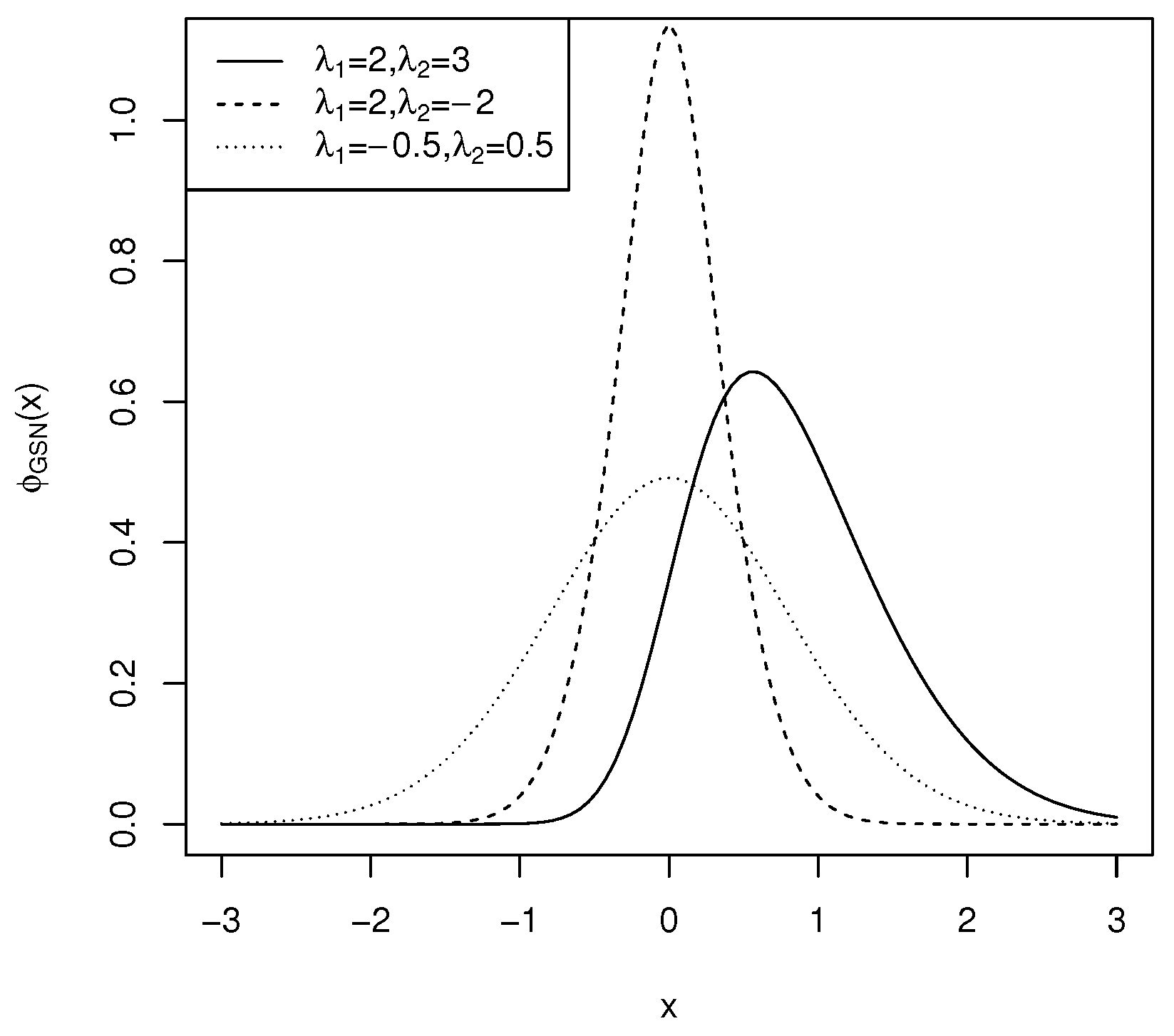
In the special case where ${\lambda }_1=-{\lambda }_2=\lambda$, the density function in (1) simplifies to the generalized normal distribution $GN(\lambda ,\rho )$, given by

$${\varphi }_{GN}(x;\lambda ,\rho )=c(\lambda ,\rho )\varphi \left(x\right){\Phi }_2(\lambda x,-\lambda x,\rho ),x\in \mathbb{R},$$

(2)

where

$$c(\lambda ,\rho )={\displaystyle \frac{2\pi }{{cos}^{-1}\left(\frac{-(\rho -{\lambda }^2)}{1+{\lambda }^2}\right)}},$$

(3)

defines the normalization constant.

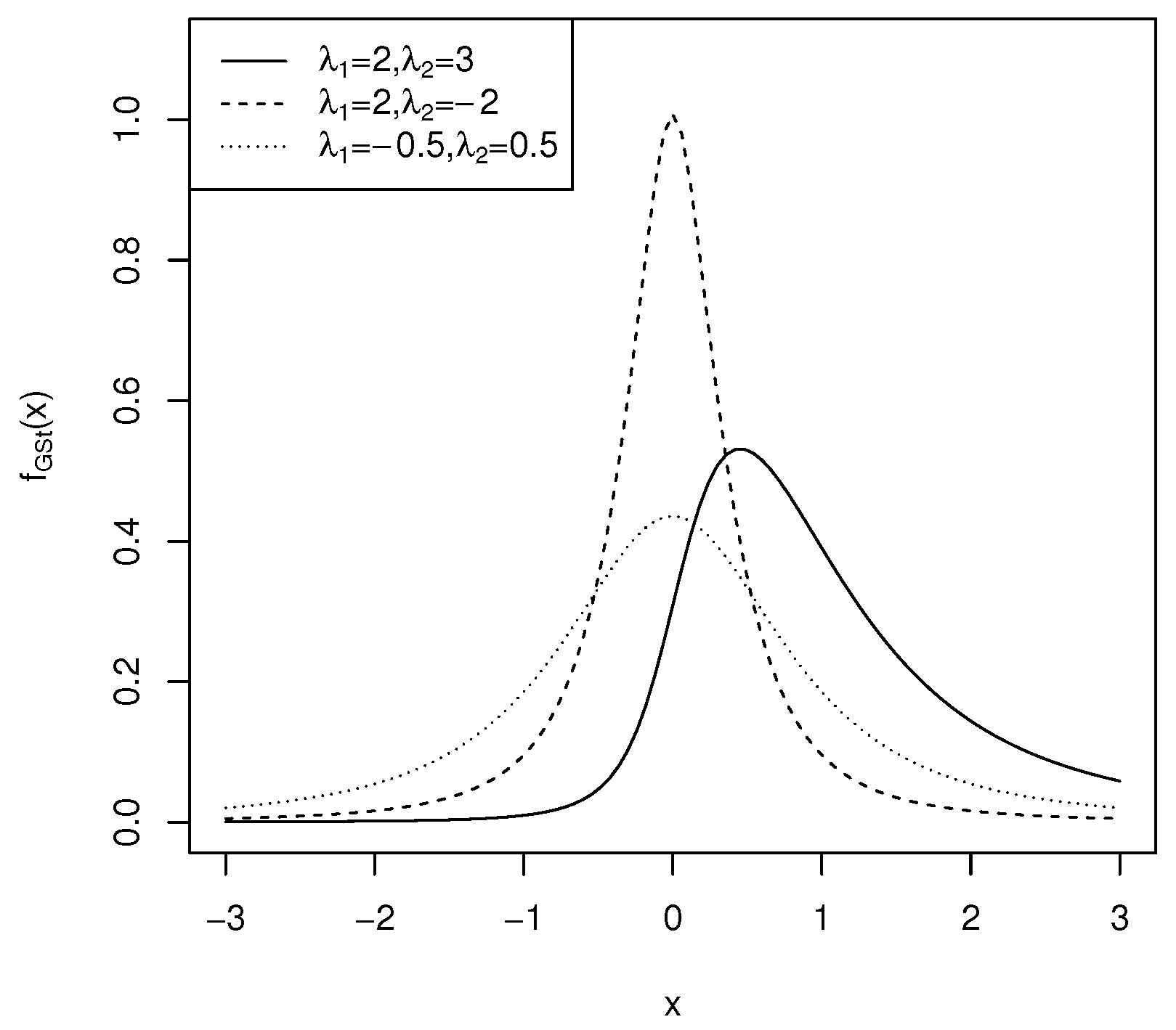
This distribution represents a symmetric distribution centered at zero as depicted in Figure 1. The capability of this distribution to retain symmetry while introducing elements of skewness makes it particularly valuable for statistical modeling applications.

Figure 1. The density function of $GSN({\lambda }_1,{\lambda }_2,\rho )$ for $\rho =0.8$.

Definition 1.

The family of skew-symmetric (-modulated) distributions is defined by the following density function [5]:

$${\varphi }_{SS}\left(x\right)=2f\left(x\right)\Pi \left(\omega \left(x\right)\right),$$

(4)

where $f(·)$ is a symmetric density function (symmetric about zero), $\omega (·)$ is an odd function, and $\Pi :\mathbb{R}\to [0,1]$ is a distribution function such that $\Pi \left(t\right)+\Pi (-t)=1$.

This definition highlights the interplay between symmetry and skewness, enabling nuanced modeling of real-world phenomena. Azzalini and Regoli [6] explored various properties of skew-symmetric (-modulated) distributions, contributing significantly to the theoretical framework essential for practical applications. Several studies have investigated skew-symmetric distributions, including that of Nadarajah and Kotz [7], which introduced a family of skew-symmetric normal distributions characterized by the density function $2\varphi \left(x\right)F\left(\alpha x\right)$, where $\alpha$ is a real constant and $F(·)$ is an absolutely continuous distribution function with a symmetric density. By utilizing distribution functions such as normal, Student’s t, Laplace, logistic, and uniform distributions for $F(·)$, the authors demonstrated the versatility of skew-symmetric models across different contexts.

Gupta and Chang [8] examined a class of multivariate skew distributions, emphasizing the importance of skewness in multivariate data analysis. Meanwhile, Gomez et al. [9] studied a general family of skew-symmetric distributions generated by the normal distribution’s cumulative distribution function, further expanding the theoretical landscape of these distributions. Additionally, Nekoukhou and Alamatsaz [10] introduced a family of skew-symmetric Laplace distributions, which have practical applications in fields such as finance and risk management. Salehi and Azzalini [11] considered a Kotz-type distribution, where the tail weight and degree of peakedness is regulated by two parameters instead of a single one, and with a built symmetry-modulated Kotz-type distribution. They made statistical inference based on the likelihood function on three real data sets.

In this paper, we aim to introduce a three-parameter skew-symmetric generalized normal, and a four-parameter skew-symmetric generalized t distributions as two new flexible models with wider ranges of skewness. The remainder of this paper is structured as follows: Section 2 presents the skew-symmetric generalized normal distribution and discusses its key properties. Section 3 then introduces the skew-symmetric generalized t distribution, providing a recurrence relation and an explicit form for its cumulative distribution function (cdf). Section 4 offers numerical examples, including a simulation study and an analysis of real data. Finally, the paper concludes in Section 5.

2. Skew-Symmetric Generalized Normal Distribution

The three-parameter skew-symmetric generalized normal distribution, denoted as $SSGN(\lambda ,\rho ,\alpha )$, is derived by substituting the symmetric density function $f(.)$ from (2) into (4). In this formulation, we utilize the standard normal distribution function, represented as $\Pi (.)$, and define the weighting function $\omega \left(x\right)=\alpha x$. This approach allows us to capture the skewness and symmetry properties inherent in the distribution.

The density function for the $SSGN$ is expressed mathematically as follows:

$${\varphi }_{SSGN}(x;\lambda ,\rho ,\alpha )=2c(\lambda ,\rho )\varphi \left(x\right){\Phi }_2(\lambda x,-\lambda x,\rho )\Phi \left(\alpha x\right),x\in \mathbb{R},$$

(5)

where $\alpha \in \mathbb{R}$, $\lambda \in \mathbb{R}$, and $\rho$ ($\left|\rho \right|<1$) are shape parameters, and $c(\lambda ,\rho )$ is a normalization constant defined in (3). This formulation highlights the interplay between the parameters $\lambda$, $\rho$, and $\alpha$, which together characterize the shape and behavior of the distribution.

In cases where $\rho =0$, the density function of the $SSGN$ simplifies significantly, leading to the following expression:

$${\varphi }_{SSGN}(x;\lambda ,\alpha )={\displaystyle \frac{4\pi }{{cos}^{-1}\left(\frac{{\lambda }^2}{1+{\lambda }^2}\right)}}\varphi \left(x\right)\Phi \left(\lambda x\right)\Phi (-\lambda x)\Phi \left(\alpha x\right),x\in \mathbb{R}.$$

(6)

This simplification exposes the core structure of the distribution in the absence of the correlation parameter, facilitating a clearer analysis of the effects and roles of the remaining parameters.

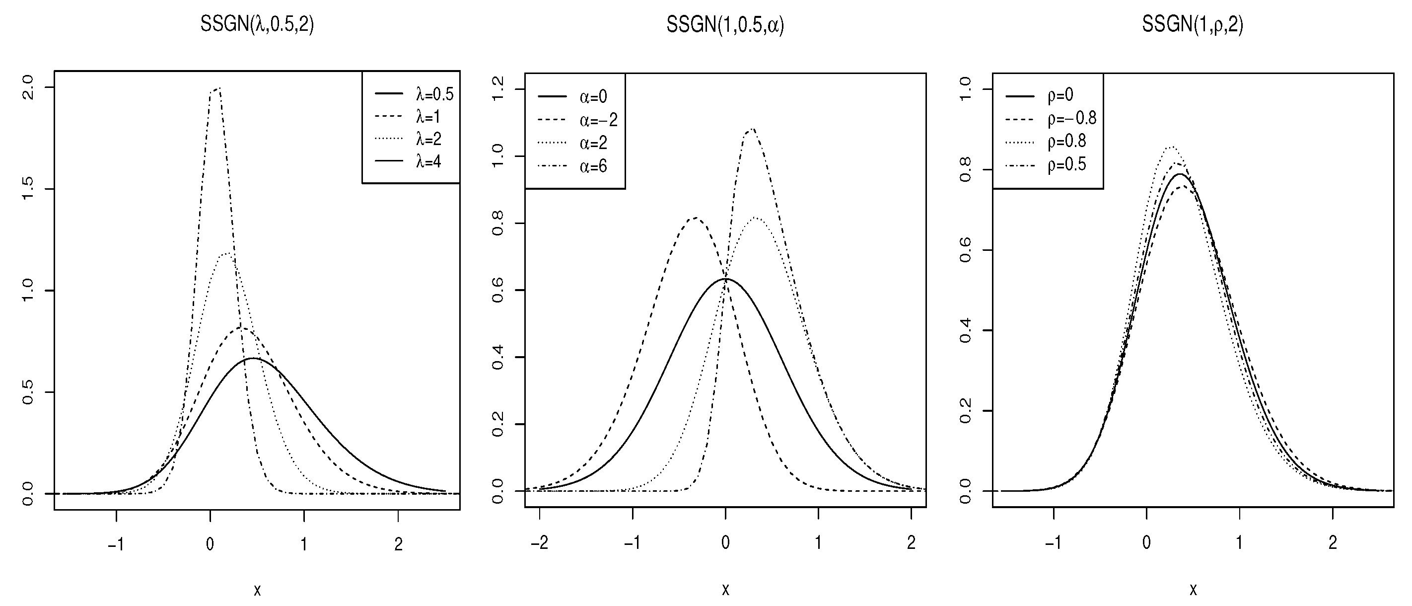
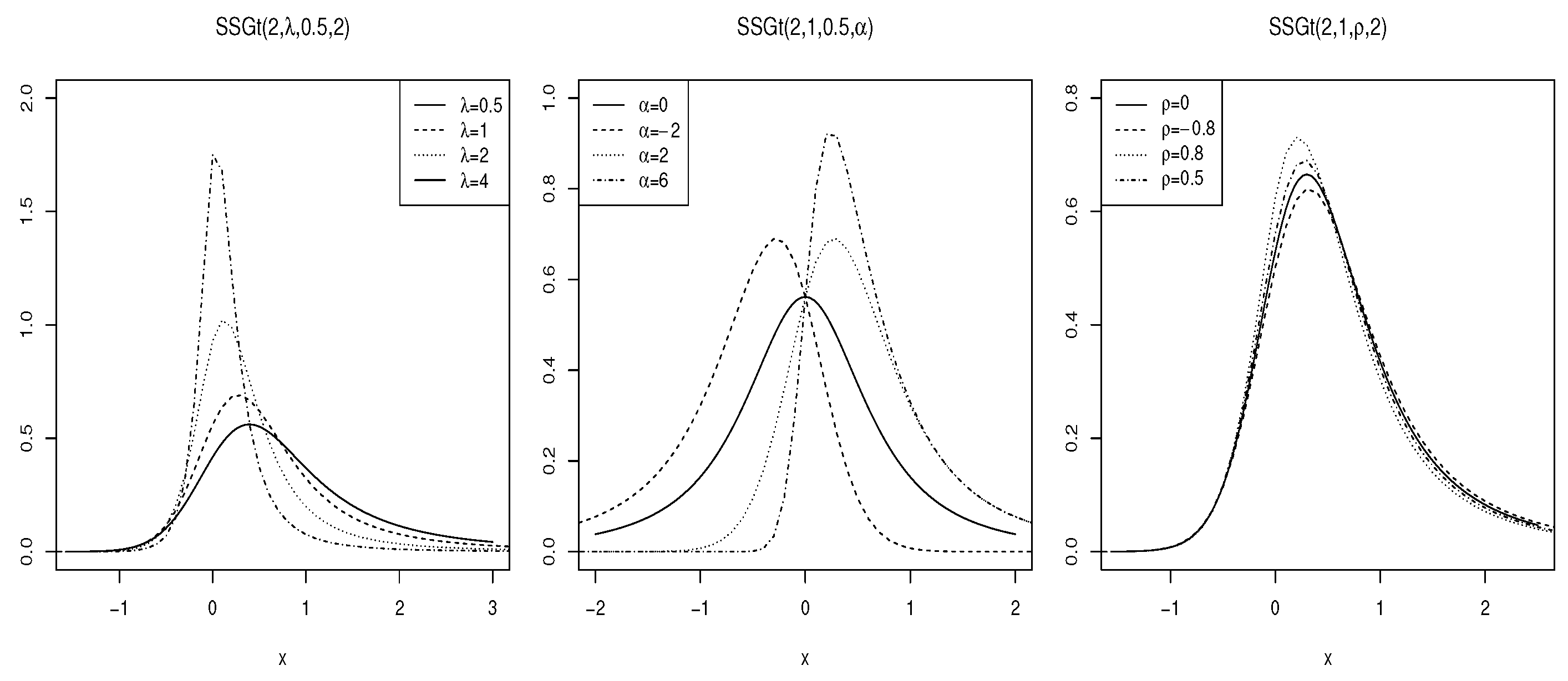
The graphical representation of the density function of $SSGN$ for various parameter values is illustrated in Figure 2. These plots provide valuable insights into how the parameters $\lambda$, $\rho$, and $\alpha$ influence the shape and characteristics of the $SSGN$. By examining these plots, one can observe the effects of skewness and kurtosis, which are critical in understanding the distribution’s behavior in practical applications.

Figure 2. The density function of $SSGN(\lambda ,\rho ,\alpha )$ for some choices of the parameters.

Overall, the $SSGN$ serves as a versatile model in statistical analysis, accommodating a range of data characteristics through its parameterization, and the visualizations further enhance our comprehension of its properties.

Remark 2.

The following results are readily obtained:

1. 

$SSGN(0,0,0)\equiv N(0,1)$

2. 

$SSGN(0,0,\alpha )\equiv SN\left(\alpha \right)$

3. 

$SSGN(\lambda ,\rho ,0)\equiv GN(\lambda ,\rho )$

4. 

$SSGN(-\lambda ,\rho ,\alpha )\equiv SSGN(\lambda ,\rho ,\alpha )$ (Thus, $SSGN$ is not identifiable.)

5. 

If $X\sim SSGN(\lambda ,\rho ,\alpha )$, then $-X\sim SSGN(\lambda ,\rho ,-\alpha )$

6. 

If $X\sim SSGN(\lambda ,\rho ,\alpha )$, then $X\stackrel{d}{=}U|\alpha \left(U\right)>Z$, where $Z\sim N(0,1)$, $U\sim GN(\lambda ,\rho )$, and $Z\perp U$.

Moments

In this section, we analyze the skewness and kurtosis of the three-parameter $SSGN$ distribution. To facilitate this analysis, we first derive the moment-generating function (MGF) of the $SSGN$.

Theorem 1.

The moment-generating function of $SSGN(\lambda ,\rho ,\alpha )$ is given by

$$M(t;\lambda ,\rho ,\alpha )=2c(\lambda ,\rho )exp\left({\displaystyle \frac{t^2}{2}}\right){\Phi }_3\left({\displaystyle \frac{\lambda t}{\sqrt{1+{\lambda }^2}}},{\displaystyle \frac{-\lambda t}{\sqrt{1+{\lambda }^2}}},{\displaystyle \frac{\alpha t}{\sqrt{1+{\alpha }^2}}},\mathbf{R}\right),$$

(7)

where

$$\mathbf{R}=\left[\begin{array}{ccc}1& {\rho }_{12}& {\rho }_{13}\\ & 1& -{\rho }_{13}\\ & & 1\end{array}\right]=\left[\begin{array}{ccc}1& {\displaystyle \frac{\rho -{\lambda }^2}{1+{\lambda }^2}}& {\displaystyle \frac{\lambda \alpha }{\sqrt{1+{\lambda }^2}\sqrt{1+{\alpha }^2}}}\\ & 1& {\displaystyle \frac{-\lambda \alpha }{\sqrt{1+{\lambda }^2}\sqrt{1+{\alpha }^2}}}\\ & & 1\end{array}\right].$$

(8)

Proof. 

To derive the moment-generating function, we start with the integral representation of the MGF:

$$\begin{array}{ccc}\hfill M(t;\lambda ,\rho ,\alpha )& =& 2c(\lambda ,\rho ){\int }_{-\infty }^{\infty }{e}^{tx}\varphi \left(x\right){\Phi }_2(\lambda x,-\lambda x,\rho )\Phi \left(\alpha x\right)dx\hfill \\ & =& 2c(\lambda ,\rho )e^{{\displaystyle \frac{t^2}{2}}}{\int }_{-\infty }^{\infty }\varphi (x-t){\Phi }_2(\lambda x,-\lambda x,\rho )\Phi \left(\alpha x\right)dx\hfill \\ & =& 2c(\lambda ,\rho )e^{{\displaystyle \frac{t^2}{2}}}{\int }_{-\infty }^{\infty }\varphi \left(z\right){\Phi }_2(\lambda (z+t),-\lambda (z+t),\rho )\Phi \left(\alpha (z+t)\right)dz\hfill \\ & =& 2c(\lambda ,\rho )e^{{\displaystyle \frac{t^2}{2}}}E\left({\Phi }_2(\lambda (z+t),-\lambda (z+t),\rho )\Phi \left(\alpha (z+t)\right)\right)\hfill \\ & =& 2c(\lambda ,\rho )e^{{\displaystyle \frac{t^2}{2}}}P(Y_1-\lambda Z<\lambda t,Y_2+\lambda Z<-\lambda t,Y_3-\alpha Z<\alpha t)\hfill \\ & =& 2c(\lambda ,\rho )e^{{\displaystyle \frac{t^2}{2}}}{\Phi }_3\left({\displaystyle \frac{\lambda t}{\sqrt{1+{\lambda }^2}}},{\displaystyle \frac{-\lambda t}{\sqrt{1+{\lambda }^2}}},{\displaystyle \frac{\alpha t}{\sqrt{1+{\alpha }^2}}},\mathbf{R}\right),\hfill \end{array}$$

where ${(Y_1,Y_2)}^T$ follows a bivariate normal distribution $N_2(0,0,1,1,\rho )$, which is independent of $Y_3$ and Z, where Z is independently and identically distributed as $N(0,1)$. □

The derivatives of the moment-generating function, evaluated at $t=0$, provide the moments of the $SSGN(\lambda ,\rho ,\alpha )$. To aid in this process, we present the following lemma.

Lemma 1.

Let $\mathit{\gamma }, \mathit{\beta }\in {\mathbb{R}}^p$ defined as $\mathit{\gamma }={\left({\gamma }_1,{\gamma }_2,\cdots ,{\gamma }_p\right)}^T$ and $\mathit{\beta }={\left({\beta }_1,{\beta }_2,\cdots ,{\beta }_p\right)}^T$. Let $\Sigma =\left({\sigma }_{ij}\right)$ denote a $p\times p$ positive definite covariance matrix. Furthermore, we assume that for $i=1,2,\dots ,p$, $\mathit{\gamma }, \mathit{\beta }$, and Σ are partitioned as follows:

$$\mathit{\gamma }=\left(\begin{array}{c}{\gamma }_i\\ {\mathit{\gamma }}_{-i}\end{array}\right),\mathit{\beta }=\left(\begin{array}{c}{\beta }_i\\ {\mathit{\beta }}_{-i}\end{array}\right),\Sigma =\left(\begin{array}{cc}{\sigma }_{ii}& {\mathit{\sigma }}_{-ii}^T\\ {\mathit{\sigma }}_{-ii}& {\Sigma }_{-i-i}\end{array}\right),$$

then, for $s\in \mathbb{R}$ we have [12]

$$\begin{array}{ccc}\hfill {\displaystyle \frac{\partial }{\partial s}}{\Phi }_p\left(\mathit{\gamma }s+\mathit{\beta };\Sigma \right)& =& \sum _{i=1}^p\left({\displaystyle \frac{{\gamma }_i}{\sqrt{{\sigma }_{ii}}}}\right)\varphi \left({\displaystyle \frac{{\gamma }_{i}s+{\beta }_i}{\sqrt{{\sigma }_{ii}}}}\right)\hfill \\ & & \times {\Phi }_{p-1}\left(\left({\mathit{\gamma }}_{-i}-{\displaystyle \frac{{\gamma }_i}{{\sigma }_{ii}}}{\mathit{\sigma }}_{-ii}\right)s+\left({\mathit{\beta }}_{-i}-{\displaystyle \frac{{\beta }_i}{{\sigma }_{ii}}}{\mathit{\sigma }}_{-ii}\right);{\Sigma }_{-i|i}\right).\hfill \end{array}$$

where ${\mathit{\gamma }}_{-i}={\left({\gamma }_1,\cdots ,{\gamma }_{i-1},{\gamma }_{i+1},\dots ,{\gamma }_p\right)}^T$ and ${\Sigma }_{-i|i}={\Sigma }_{-i-i}-{\displaystyle \frac{{\mathit{\sigma }}_{-ii}{\mathit{\sigma }}_{-ii}^T}{{\sigma }_{ii}}}$.

The first four moments of $SSGN$ are expressed as follows:

$$\begin{array}{cc}\hfill E\left(X\right)& ={\displaystyle \frac{2c(\lambda ,\rho )}{\sqrt{2\pi }}}\left\{{\displaystyle \frac{-{\gamma }_1}{\pi }}{sin}^{-1}{\displaystyle \frac{{\rho }_{13}+{\rho }_{12}{\rho }_{13}}{\sqrt{1-{\rho }_{12}^2}\sqrt{1-{\rho }_{13}^2}}}+{\gamma }_2\left({\displaystyle \frac{1}{4}}+{\displaystyle \frac{1}{2\pi }}{sin}^{-1}{\displaystyle \frac{{\rho }_{12}+{\rho }_{13}^2}{1-{\rho }_{13}^2}}\right)\right\},\hfill \end{array}$$

(9)

$$\begin{array}{cc}\hfill E\left(X^2\right)& =1-{\displaystyle \frac{{\lambda }^{2}c(\lambda ,\rho )(1+\rho )}{\pi (1+{\lambda }^2)\sqrt{1-{\rho }^2+2{\lambda }^2+2\rho {\lambda }^2}}},\hfill \end{array}$$

(10)

$$\begin{array}{cc}\hfill E\left(X^3\right)& ={\displaystyle \frac{2c(\lambda ,\rho )}{\sqrt{2\pi }}}\left\{{\displaystyle \frac{{\gamma }_1^3-3{\gamma }_1}{\pi }}{sin}^{-1}{\displaystyle \frac{{\rho }_{13}+{\rho }_{12}{\rho }_{13}}{\sqrt{1-{\rho }_{12}^2}\sqrt{1-{\rho }_{13}^2}}}-({\gamma }_2^3-3{\gamma }_2)\left({\displaystyle \frac{1}{4}}+{\displaystyle \frac{1}{2\pi }}{sin}^{-1}{\displaystyle \frac{{\rho }_{12}+{\rho }_{13}^2}{1-{\rho }_{13}^2}}\right)\right.\hfill \\ \hfill & \left.-{\displaystyle \frac{{\gamma }_1}{\pi }}\left({\displaystyle \frac{A({\gamma }_1+{\gamma }_1{\rho }_{12})}{\sqrt{1-{\rho }_{12}^2}}}-{\displaystyle \frac{B({\gamma }_2-{\gamma }_1{\rho }_{13})}{\sqrt{1-{\rho }_{13}^2}}}\right)+{\displaystyle \frac{C{\gamma }_2({\gamma }_1-{\gamma }_2{\rho }_{13})}{\pi \sqrt{1-{\rho }_{13}^2}}}\right\},\hfill \end{array}$$

(11)

$$\begin{array}{cc}\hfill E\left(X^4\right)& =3+{\displaystyle \frac{c(\lambda ,\rho )(1+\rho )}{\pi (1+{\lambda }^2)\sqrt{1-{\rho }^2+2{\lambda }^2+2\rho {\lambda }^2}}}\left({\displaystyle \frac{3{\lambda }^4}{1+{\lambda }^2}}+{\displaystyle \frac{{\lambda }^4(1+\rho )}{(1+{\lambda }^2)(1+2{\lambda }^2-\rho )}}-6{\lambda }^2\right),\hfill \end{array}$$

(12)

where ${\gamma }_1={\displaystyle \frac{\lambda }{\sqrt{1+{\lambda }^2}}}$, ${\gamma }_2={\displaystyle \frac{\alpha }{\sqrt{1+{\alpha }^2}}}$, and

$$\begin{array}{cc}\hfill A& ={\displaystyle \frac{1}{\sqrt{1-{\rho }_{13}^2-\frac{{({\rho }_{13}+{\rho }_{12}{\rho }_{13})}^2}{1-{\rho }_{12}^2}}}}\left({\gamma }_2-{\gamma }_1{\rho }_{13}-{\displaystyle \frac{({\gamma }_1+{\gamma }_1{\rho }_{12})({\rho }_{13}+{\rho }_{12}{\rho }_{13})}{(1-{\rho }_{12}^2)}}\right),\hfill \end{array}$$

$$\begin{array}{cc}\hfill B& ={\displaystyle \frac{1}{\sqrt{1-{\rho }_{12}^2-\frac{{({\rho }_{13}+{\rho }_{12}{\rho }_{13})}^2}{1-{\rho }_{13}^2}}}}\left(-{\gamma }_1-{\gamma }_1{\rho }_{12}+{\displaystyle \frac{({\gamma }_2-{\gamma }_1{\rho }_{13})({\rho }_{13}+{\rho }_{12}{\rho }_{13})}{(1-{\rho }_{13}^2)}}\right),\hfill \end{array}$$

$$\begin{array}{cc}\hfill C& ={\displaystyle \frac{1}{\sqrt{1-{\rho }_{13}^2-\frac{{({\rho }_{12}+{\rho }_{13}^2)}^2}{1-{\rho }_{13}^2}}}}\left(-{\gamma }_1+{\gamma }_2{\rho }_{13}-{\displaystyle \frac{({\gamma }_1-{\gamma }_2{\rho }_{13})({\rho }_{12}+{\rho }_{13}^2)}{(1-{\rho }_{13}^2)}}\right).\hfill \end{array}$$

The skewness and kurtosis of the $SSGN$ can be derived from Equations (9)–(12) as follows:

$$\begin{array}{c}\hfill CS={\displaystyle \frac{E\left(X^3\right)-3E\left(X\right)E\left(X^2\right)+2E^3\left(X\right)}{Va{r}^{3/2}\left(X\right)}},\end{array}$$

(13)

$$\begin{array}{c}\hfill CK={\displaystyle \frac{E\left(X^4\right)-4E\left(X\right)E\left(X^3\right)+6E^2\left(X\right)E\left(X^2\right)-3E^4\left(X\right)}{Va{r}^2\left(X\right)}}-3,\end{array}$$

(14)

where

$$\begin{array}{c}\hfill Var\left(X\right)=1-{\displaystyle \frac{{\lambda }^{2}c(\lambda ,\rho )(1+\rho )}{\pi (1+{\lambda }^2)\sqrt{1-{\rho }^2+2{\lambda }^2+2\rho {\lambda }^2}}}-E^2\left(X\right).\end{array}$$

(15)

The plots illustrating the skewness and kurtosis of $SSGN$ for various parameter values are presented in Figure 3 and Figure 4, respectively.

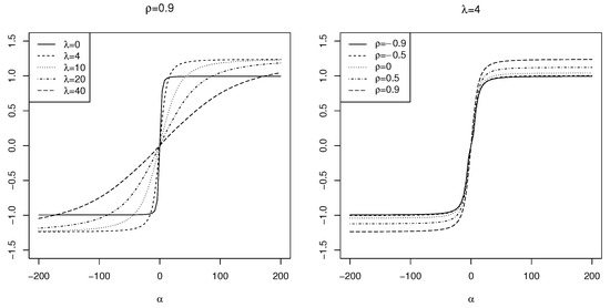
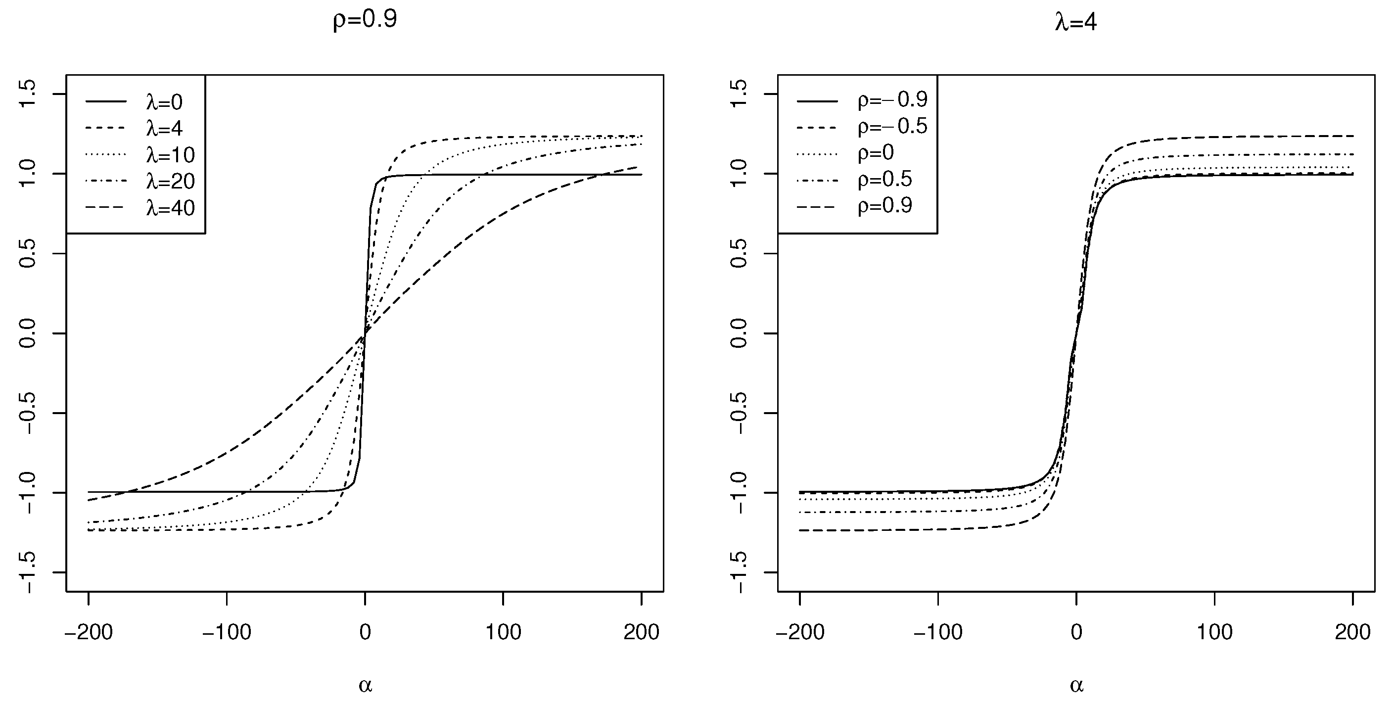
Figure 3. The skewness of $SSGN(\lambda ,\rho ,\alpha )$ for the selected parameter values.

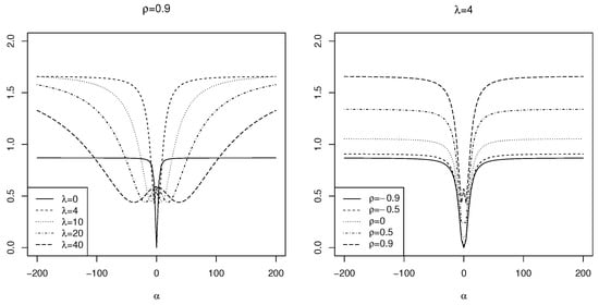
Figure 4. The kurtosis of $SSGN(\lambda ,\rho ,\alpha )$ for the selected parameter values.

As shown in Figure 3, the skewness of the $SSGN$ increases with higher values of $\alpha$ and $\rho$, indicating a greater asymmetry in the distribution. Specifically, the maximum skewness occurs at $\lambda =3.46878$, resulting in a value of $1.2382$. In contrast, Figure 4 illustrates that the kurtosis initially decreases as $\left|\alpha \right|$ increases, before rising again. The peak kurtosis value is observed at $1.6648$ for $\lambda =4.0195$. This behavior highlights the capacity of $SSGN$ to model data with varying levels of asymmetry and peakedness, providing a flexible framework for statistical analysis.

3. Skew-Symmetric Generalized t Distribution

Jamalizadeh and Balakrishnan [3] defined a four-parameter generalized skew-t distribution, $GSt(\nu ,{\lambda }_1,{\lambda }_2,\rho )$, with the following density function:

$$f_{GSt}(x;\nu ,{\lambda }_1,{\lambda }_2,\rho )={\displaystyle \frac{2\pi }{{cos}^{-1}\left(\frac{-(\rho +{\lambda }_1{\lambda }_2)}{\sqrt{1+{\lambda }_1^2}\sqrt{1+{\lambda }_2^2}}\right)}}g(x;\nu )G_2\left({\lambda }_{1}x\sqrt{{\displaystyle \frac{1+\nu }{\nu +x^2}}},{\lambda }_{2}x\sqrt{{\displaystyle \frac{1+\nu }{\nu +x^2}}};\rho ,\nu +1\right),$$

(16)

where $x\in \mathbb{R}$, $g(·;\nu )$ is the density function of the t distribution with $\nu$ degrees of freedom, and $G_2(·,·;\rho ,\nu )$ represents the distribution function of the standard bivariate t distribution with correlation $\rho$ (where $\left|\rho \right|<1$) and $\nu +1$ degrees of freedom.

Remark 3.

For the special case ${\lambda }_1=-{\lambda }_2=\lambda$, the density function (16) reduces to $Gt(\nu ,\lambda ,\rho )$ with the following density function:

$$f_{Gt}(x;\nu ,\lambda ,\rho )=c(\lambda ,\rho )g(x;\nu )G_2\left(\lambda x\sqrt{{\displaystyle \frac{1+\nu }{\nu +x^2}}},-\lambda x\sqrt{{\displaystyle \frac{1+\nu }{\nu +x^2}}};\rho ,\nu +1\right),x\in \mathbb{R},$$

(17)

where $c(\lambda ,\rho )$ is defined in (3).

This is a symmetric distribution, centered at 0, as illustrated in Figure 5.

Figure 5. The density function of $GSt(\nu ,{\lambda }_1,{\lambda }_2,\rho )$ for $\nu =2,\rho =0.8$.

The four-parameter skew-symmetric generalized t distribution, $SSGt(\nu ,\lambda ,\rho ,\alpha )$, is obtained by substituting (17) into (4) as a symmetric density function $f(.)$, using the standard normal distribution function $\Pi (.)$ and $\omega \left(x\right)=\alpha x$. The density function of $SSGt$ is given by

$$f_{SSGt}(x;\nu ,\lambda ,\rho ,\alpha )=2c(\lambda ,\rho )g(x;\nu )G_2\left(\lambda x\sqrt{{\displaystyle \frac{1+\nu }{\nu +x^2}}},-\lambda x\sqrt{{\displaystyle \frac{1+\nu }{\nu +x^2}}};\rho ,\nu +1\right)\Phi \left(\alpha x\right),x\in \mathbb{R},$$

(18)

where $\alpha \in \mathbb{R}$, $\lambda \in \mathbb{R}$, $\rho$ ($\left|\rho \right|<1$) are shape parameters, $\nu \in {\mathbb{R}}^{+}$ is the tail parameter, and $c(\lambda ,\rho )$ is defined in (3). When $\rho =0$, the density function of $SSGt$ becomes

$$f_{SSGt}(x;\nu ,\lambda ,\alpha )={\displaystyle \frac{4\pi }{{cos}^{-1}\left(\frac{{\lambda }^2}{1+{\lambda }^2}\right)}}g(x;\nu )G\left(\lambda x\sqrt{{\displaystyle \frac{1+\nu }{\nu +x^2}}};\nu +1\right)G\left(-\lambda x\sqrt{{\displaystyle \frac{1+\nu }{\nu +x^2}}};\rho ,\nu +1\right)\Phi \left(\alpha x\right).$$

(19)

The plots of the density function of $SSGt$ for various parameter values are shown in Figure 6.

Figure 6. The density function of $SSGt(\nu ,\lambda ,\rho ,\alpha )$ for various parameter choices.

Remark 4.

The following results are readily obtained:

1. 

$SSGt(\nu ,0,0,0)\equiv t\left(\nu \right)$

2. 

$SSGt(\nu ,0,0,\alpha )\equiv St(\nu ,\alpha )$

3. 

$SSGt(\nu ,\lambda ,\rho ,0)\equiv Gt(\nu ,\lambda ,\rho )$

4. 

$SSGt(\nu ,-\lambda ,\rho ,\alpha )\equiv SSGt(\nu ,\lambda ,\rho ,\alpha )$ (Thus, $SSGt$ is not identifiable.)

5. 

If $X\sim SSGt(\nu ,\lambda ,\rho ,\alpha )$, then $-X\sim SSGt(\nu ,\lambda ,\rho ,-\alpha )$

6. 

If $X\sim SSGt(\nu ,\lambda ,\rho ,\alpha )$, then $X\stackrel{d}{=}U|\alpha \left(U\right)>Z$, where $Z\sim N(0,1)$, $U\sim GN(\lambda ,\rho )$, and $Z\perp U$.

Remark 5.

If $X\sim SSGt(\nu ,\lambda ,\rho ,\alpha )$, then $X\stackrel{d}{=}{W}^{-1/2}Z$, where $W\sim {\chi }_{\nu }^2/\nu$, $Z\sim SSGN(\lambda ,\rho ,\alpha )$, and $W\perp Z$. Thus, the integral form of the cumulative distribution function (cdf) of the $SSGt$ distribution is as follows:

$$\begin{array}{ccc}\hfill F_{SSGt}\left(t;\nu ,\lambda ,\rho ,\alpha \right)& =& E\left[{\Phi }_{SSGN}\left(t\sqrt{W};\lambda ,\rho ,\alpha \right)\right]\hfill \\ & =& 2\sqrt{\pi }{C}_{\nu }{\int }_0^{\infty }{x}^{\nu -1}\varphi \left(x\right){\Phi }_{SSGN}\left({\displaystyle \frac{tx}{\sqrt{\nu }}};\lambda ,\rho ,\alpha \right)dx,\hfill \end{array}$$

(20)

where

$$C_{\nu }={\displaystyle \frac{1}{\Gamma \left(\frac{\nu }{2}\right)2^{\left(\nu -1\right)/2}}}.$$

Amiri et al. [13] obtained efficient recursive computational algorithms for multivariate t and multivariate unified skew-t distributions. Also, Salehi et al. [12] obtained recurrence relations for the cdf and the density function of the generalized skew two-piece skew-t distribution. Here, we intend to achieve to a recurrence relation for the cdf of the $SSGt$ distribution from the integration form given by (20).

Theorem 2.

The following recurrence relation holds for all $\nu >1$:

$$\begin{array}{cc}\hfill & F_{SSGt}\left(t;\nu +1,\lambda ,\rho ,\alpha \right)=F_{SSGt}\left(\sqrt{{\displaystyle \frac{\nu -1}{\nu +1}}}t;\nu -1,\lambda ,\rho ,\alpha \right)\hfill \\ \hfill & +2c\left(\lambda ,\rho \right)h\left(t;\nu +1,\nu -1\right)G_3\left({\displaystyle \frac{\sqrt{\nu }\lambda t}{\sqrt{\nu +1+t^2}}},{\displaystyle \frac{-\sqrt{\nu }\lambda t}{\sqrt{\nu +1+t^2}}},{\displaystyle \frac{\sqrt{\nu }\alpha t}{\sqrt{\nu +1+t^2}}};\nu ,{\mathbf{R}}^{*}\right),\hfill \end{array}$$

(21)

where $h\left(t;{\nu }_1,{\nu }_2\right)={\displaystyle \frac{t}{\sqrt{{\nu }_1{\nu }_2}}}g\left(\sqrt{{\displaystyle \frac{{\nu }_2}{{\nu }_1}}}t;{\nu }_2\right)$, $G_3(·,·,·;\nu ,{\mathbf{R}}^{*})$ stands for the cdf of the trivariate Student’s t distribution with ν degrees of freedom and the correlation matrix

$${\mathbf{R}}^{*}=\left[\begin{array}{ccc}1& \rho & 0\\ \rho & 1& 0\\ 0& 0& 1\end{array}.\right]$$

Proof. 

From (20) and upon integrating by parts, the cdf of $SSGt$ distribution with $\nu +1$ degrees of freedom is readily obtained as

$$\begin{array}{ccc}\hfill F_{SSGt}\left(t;\nu +1,\lambda ,\rho ,\alpha \right)& =& 2\sqrt{\pi }{C}_{\nu +1}{\int }_0^{\infty }{x}^{\nu }\varphi \left(x\right){\Phi }_{SSGN}\left({\displaystyle \frac{tx}{\sqrt{\nu +1}}};\lambda ,\rho ,\alpha \right)dx\hfill \\ & =& F_{SSGt}\left(\sqrt{{\displaystyle \frac{\nu -1}{\nu +1}}}t;\nu -1,\lambda ,\rho ,\alpha \right)\hfill \\ \hfill & & +2\sqrt{\pi }{C}_{\nu +1}{\int }_0^{\infty }{x}^{\nu -1}\varphi \left(x\right)\left\{{\displaystyle \frac{\partial }{\partial x}}{\Phi }_{SSGN}\left({\displaystyle \frac{tx}{\sqrt{\nu +1}}};\lambda ,\rho ,\alpha \right)\right\}dx.\hfill \end{array}$$

(22)

Now, the second part of the right-hand side (RHS) of (22) is simplified to

$$\begin{array}{cc}\hfill RHS& =2\sqrt{\pi }{C}_{\nu +1}{\displaystyle \frac{t}{\sqrt{\nu +1}}}{\int }_0^{\infty }{x}^{\nu -1}\varphi \left(x\right){\varphi }_{SSGN}\left({\displaystyle \frac{tx}{\sqrt{\nu +1}}};\lambda ,\rho ,\alpha \right)dx\hfill \\ \hfill & =2\sqrt{\pi }{C}_{\nu +1}{\displaystyle \frac{2c\left(\lambda ,\rho \right)t}{\sqrt{\nu +1}}}{\int }_0^{\infty }{x}^{\nu -1}\varphi \left(x\right)\varphi \left({\displaystyle \frac{tx}{\sqrt{\nu +1}}}\right){\Phi }_2\left({\displaystyle \frac{\lambda tx}{\sqrt{\nu +1}}},{\displaystyle \frac{-\lambda tx}{\sqrt{\nu +1}}};\rho \right)\Phi \left({\displaystyle \frac{\alpha tx}{\sqrt{\nu +1}}}\right)dx\hfill \\ \hfill & ={\displaystyle \frac{c\left(\lambda ,\rho \right)\Gamma \left(\frac{\nu }{2}\right){\left(\nu +1\right)}^{\left(\nu -1\right)/2}}{\sqrt{\pi }\Gamma \left(\frac{\nu +1}{2}\right)}}{\displaystyle \frac{t}{{\left(\nu +1+t^2\right)}^{\nu /2}}}\hfill \\ \hfill & \times 2\sqrt{\pi }{C}_{\nu }{\int }_0^{\infty }{x}^{\nu -1}\varphi \left(x\right){\Phi }_2\left({\displaystyle \frac{\lambda tx}{\sqrt{\nu +1+t^2}}},{\displaystyle \frac{-\lambda tx}{\sqrt{\nu +1+t^2}}};\rho \right)\Phi \left({\displaystyle \frac{\alpha tx}{\sqrt{\nu +1+t^2}}}\right)dx\hfill \\ \hfill & =2c\left(\lambda ,\rho \right)h\left(t;\nu +1,\nu -1\right)\hfill \\ \hfill & \times 2\sqrt{\pi }{C}_{\nu }{\int }_0^{\infty }{x}^{\nu -1}\varphi \left(x\right){\Phi }_3\left({\displaystyle \frac{\sqrt{\nu }\lambda tx}{\sqrt{\nu }\sqrt{\nu +1+t^2}}},{\displaystyle \frac{-\sqrt{\nu }\lambda tx}{\sqrt{\nu }\sqrt{\nu +1+t^2}}},{\displaystyle \frac{\sqrt{\nu }\alpha tx}{\sqrt{\nu }\sqrt{\nu +1+t^2}}};{\mathbf{R}}^{*}\right)dx\hfill \\ \hfill & =2c\left(\lambda ,\rho \right)h\left(t;\nu +1,\nu -1\right)G_3\left({\displaystyle \frac{\sqrt{\nu }\lambda t}{\sqrt{\nu +1+t^2}}},{\displaystyle \frac{-\sqrt{\nu }\lambda t}{\sqrt{\nu +1+t^2}}},{\displaystyle \frac{\sqrt{\nu }\alpha t}{\sqrt{\nu +1+t^2}}};\nu ,{\mathbf{R}}^{*}\right).\hfill \end{array}$$

□

Remark 6.

From Theorem 2, the following results are respectively concluded for odd and even values of ν

$$\begin{array}{cc}\hfill & F_{SSGt}\left(t;\nu ,\lambda ,\rho ,\alpha \right)=F_{SSGt}\left({\displaystyle \frac{t}{\sqrt{\nu }}};1,\lambda ,\rho ,\alpha \right)\hfill \\ \hfill & +2c\left(\lambda ,\rho \right)\sum _{i=1}^{\left(\nu -1\right)/2}h\left(t;\nu ,2i-1\right)G_3\left({\displaystyle \frac{\sqrt{2i}\lambda t}{\sqrt{\nu +t^2}}},{\displaystyle \frac{-\sqrt{2i}\lambda t}{\sqrt{\nu +t^2}}},{\displaystyle \frac{\sqrt{2i}\alpha t}{\sqrt{\nu +t^2}}};2i,{\mathbf{R}}^{*}\right),\hfill \end{array}$$

(23)

and

$$\begin{array}{cc}\hfill & F_{SSGt}\left(t;\nu ,\lambda ,\rho ,\alpha \right)=F_{SSGt}\left(\sqrt{{\displaystyle \frac{2}{\nu }}}t;2,\lambda ,\rho ,\alpha \right)\hfill \\ \hfill & +2c\left(\lambda ,\rho \right)\sum _{i=2}^{\nu /2}h\left(t;\nu ,2i-2\right)G_3\left({\displaystyle \frac{\sqrt{2i-1}\lambda t}{\sqrt{\nu +t^2}}},{\displaystyle \frac{-\sqrt{2i-1}\lambda t}{\sqrt{\nu +t^2}}},{\displaystyle \frac{\sqrt{2i-1}\alpha t}{\sqrt{\nu +t^2}}};2i-1,{\mathbf{R}}^{*}\right).\hfill \end{array}$$

(24)

There is no explicit form for $F_{SSGt}\left(t;1,\lambda ,\rho ,\alpha \right)$ to be used as the starting point in (24). But an explicit form for $f_{SSGt}\left(t;1,\lambda ,\rho ,\alpha \right)$ is obtained as

$$f_{SSGt}\left(t;1,\lambda ,\rho ,\alpha \right)={\displaystyle \frac{c\left(\lambda ,\rho \right)}{\sqrt{\pi }\left(1+t^2\right)}}{G}_3\left({\displaystyle \frac{\sqrt{2}\lambda t}{\sqrt{1+t^2}}},{\displaystyle \frac{-\sqrt{2}\lambda t}{\sqrt{1+t^2}}},{\displaystyle \frac{\sqrt{2}\alpha t}{\sqrt{1+t^2}}};2,{\mathbf{R}}^{*}\right).$$

Also an explicit form for $F_{SSGt}\left(t;2,\lambda ,\rho ,\alpha \right)$ is as

$$\begin{array}{cc}\hfill & F_{SSGt}\left(t;2,\lambda ,\rho ,\alpha \right)={\Phi }_{SSGN}\left(0;\lambda ,\rho ,\alpha \right)\hfill \\ \hfill & +{\displaystyle \frac{c\left(\lambda ,\rho \right)t}{c\left(\frac{\lambda t}{\sqrt{2+t^2}},\rho \right)}}{\Phi }_{SSGN}\left(0;{\displaystyle \frac{\lambda t}{\sqrt{2+t^2}}},\rho ,{\displaystyle \frac{-\alpha t}{\sqrt{2+t^2}}}\right).\hfill \end{array}$$

Thus, a closed form for the cdf of the $SSGt$ distribution is accessible.

Moments

According to Remark 5, the $r^{th}$ moment of $X\sim SSGt(\nu ,\lambda ,\rho ,\alpha )$ can be derived as follows:

$$E\left(X^r\right)=E\left(W^{-r/2}\right)E\left(Z^r\right),$$

(25)

where

$$E\left(W^{-r/2}\right)={\displaystyle \frac{{\left(\frac{\nu }{2}\right)}^{r/2}\Gamma \left(\frac{\nu -r}{2}\right)}{\Gamma \left(\frac{\nu }{2}\right)}},\nu >r.$$

Thus, the first four moments of $SSGt$ can be obtained using the first four moments of $SSGN$ in Equations (9)–(12). Consequently, the skewness and kurtosis of $SSGt$ can be derived from Equations (13) and (14), respectively. The plots of skewness and kurtosis of $SSGt$ for various parameter values are shown in Figure 7 and Figure 8, respectively.

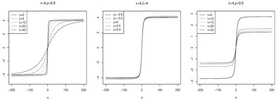
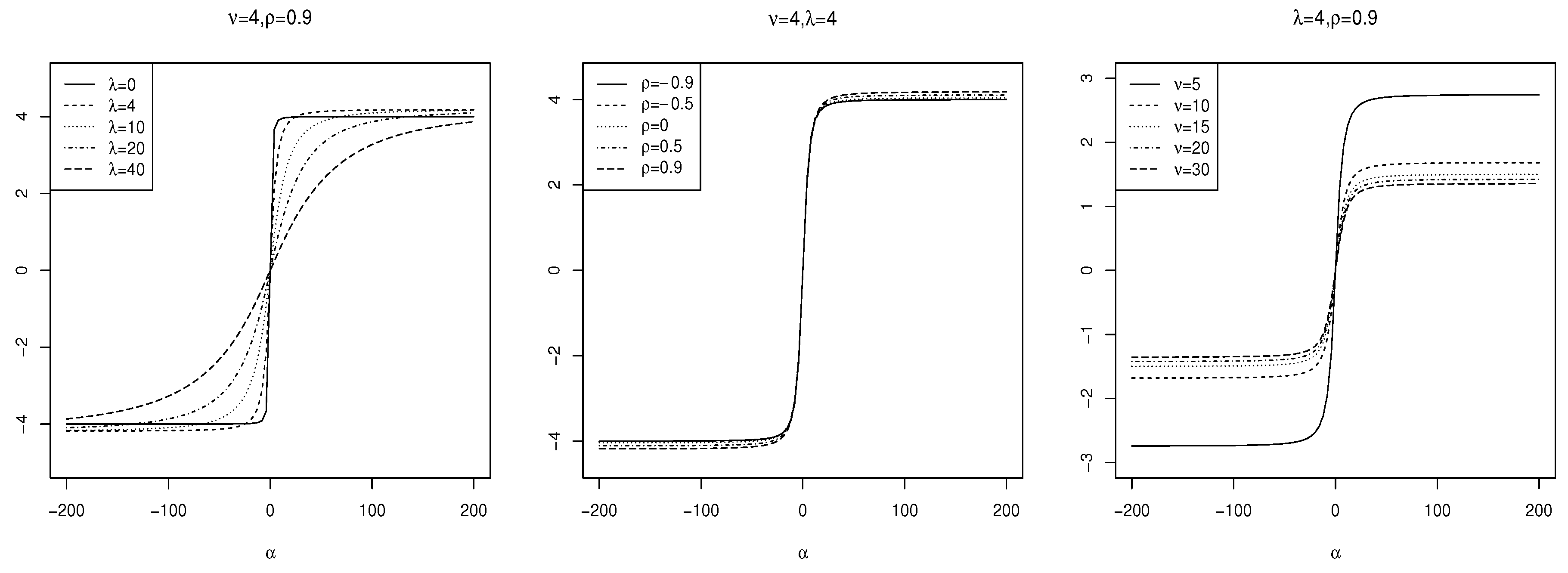
Figure 7. The skewness of $SSGt(\nu ,\lambda ,\rho ,\alpha )$ for various parameter choices.

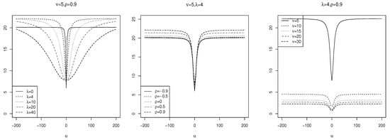
Figure 8. The kurtosis of $SSGt(\nu ,\lambda ,\rho ,\alpha )$ for various parameter choices.

As observed in Figure 7, along with the numerical optimization results, the skewness of $SSGt$ increases with increasing $\alpha$ and $\rho$ while decreasing with increasing $\nu$. The maximum skewness occurs at $\lambda =3.8114$, with a value of $4.1821$. From Figure 8, the kurtosis increases with increasing $\left|\alpha \right|$ and $\rho$ while decreasing with $\nu$. The maximum kurtosis value is $22.1327$ for $\lambda =4.5767$. Thus, the ranges of skewness and kurtosis of $SSGt$ are wider than those of $SSGN$.

4. Numerical Illustration

For practical works, the distributions proposed so far in (5) and (18) must be supplied with a location (denoted by $\mu$) and a scale (denoted by $\sigma$) parameters yielding $SSGN(\mu ,\sigma ,\lambda ,\rho ,\alpha )$ and $SSGt(\mu ,\sigma ,\nu ,\lambda ,\rho ,\alpha ,\nu )$ distributions, respectively. If we assume that the observations $\mathbf{x}=(x_1,\dots ,x_n)$ follow from the former distribution under independence conditions, then the log-likelihood function of $(\mu ,\sigma ,\lambda ,\rho ,\alpha )$ is

$$\begin{array}{ccc}\hfill l(\mu ,\sigma ,\lambda ,\rho ,\alpha )& =& nln2c(\lambda ,\rho )-nln\sigma -{\displaystyle \frac{n}{2}}ln\left(2\pi {\sigma }^2\right)-{\displaystyle \frac{1}{2{\sigma }^2}}\sum _{i=1}^n{(x_i-\mu )}^2\hfill \\ & +& \sum _{i=1}^{n}ln{\Phi }_2\left({\displaystyle \frac{\lambda (x_i-\mu )}{\sigma }},{\displaystyle \frac{-\lambda (x_i-\mu )}{\sigma }},\rho \right)+\sum _{i=1}^{n}ln\Phi \left({\displaystyle \frac{\alpha (x_i-\mu )}{\sigma }}\right).\hfill \end{array}$$

(26)

Similarly, for the $SSGt(\mu ,\sigma ,\nu ,\lambda ,\rho ,\alpha )$ distribution, we have

$$\begin{array}{ccc}\hfill l(\mu ,\sigma ,\nu ,\lambda ,\rho ,\alpha )& =& nln2c(\lambda ,\rho )-nln\sigma +nln\Gamma \left({\displaystyle \frac{\nu +1}{2}}\right)-nln\Gamma \left({\displaystyle \frac{\nu }{2}}\right)-{\displaystyle \frac{n}{2}}ln\left(\pi \nu \right)\hfill \\ & -& {\displaystyle \frac{\nu +1}{2}}\sum _{i=1}^{n}ln\left(1+{\displaystyle \frac{{(x_i-\mu )}^2}{\nu {\sigma }^2}}\right)+\sum _{i=1}^{n}ln\Phi \left({\displaystyle \frac{\alpha (x_i-\mu )}{\sigma }}\right)\hfill \\ & +& \sum _{i=1}^{n}ln{G}_2\left(\lambda \left({\displaystyle \frac{x-\mu }{\sigma }}\right)\sqrt{{\displaystyle \frac{1+\nu }{\nu +{\left(\frac{x-\mu }{\sigma }\right)}^2}}},-\lambda \left({\displaystyle \frac{x-\mu }{\sigma }}\right)\sqrt{{\displaystyle \frac{1+\nu }{\nu +{\left(\frac{x-\mu }{\sigma }\right)}^2}}};\rho ,\nu +1\right).\hfill \end{array}$$

(27)

Maximization of the log-likelihoods given by (26) and (27) which must be performed by numerical techniques lead to the maximum likelihood estimates (MLEs) of the parameters. Using the R programming environment [14], we employ a combination of the global optimizer $\mathtt{DEoptim}$ [15] and the local optimizer $\mathtt{optim}$ (with the ’L-BFGS-B’ method), available in the $\mathtt{DEoptim}$ and $\mathtt{stats}$ R packages, respectively. $\mathtt{DEoptim}$ package is based on the Differential Evolution (DE) algorithm [16], and its significant performance as a global optimization algorithm on continuous numerical minimization problems has been extensively studied [17].

4.1. Simulation Study

In this section, we intend to carry out a brief simulation study in order to investigate the behavior of the MLEs of the parameters of $SSGN(\mu ,\sigma ,\lambda ,\rho ,\alpha )$ distribution. To this end, we set some selected values as the true parameters, $\mu =0,\sigma =1,\lambda =1,\alpha =0.4,\rho =0.5$, and consider samples with different sizes, $n=100,200,500,1000,2000$, as the given observations. To generate samples from $SSGN$ distribution we employ the acceptance–rejection algorithm using the stochastic representation given by Remark 2, part 6.

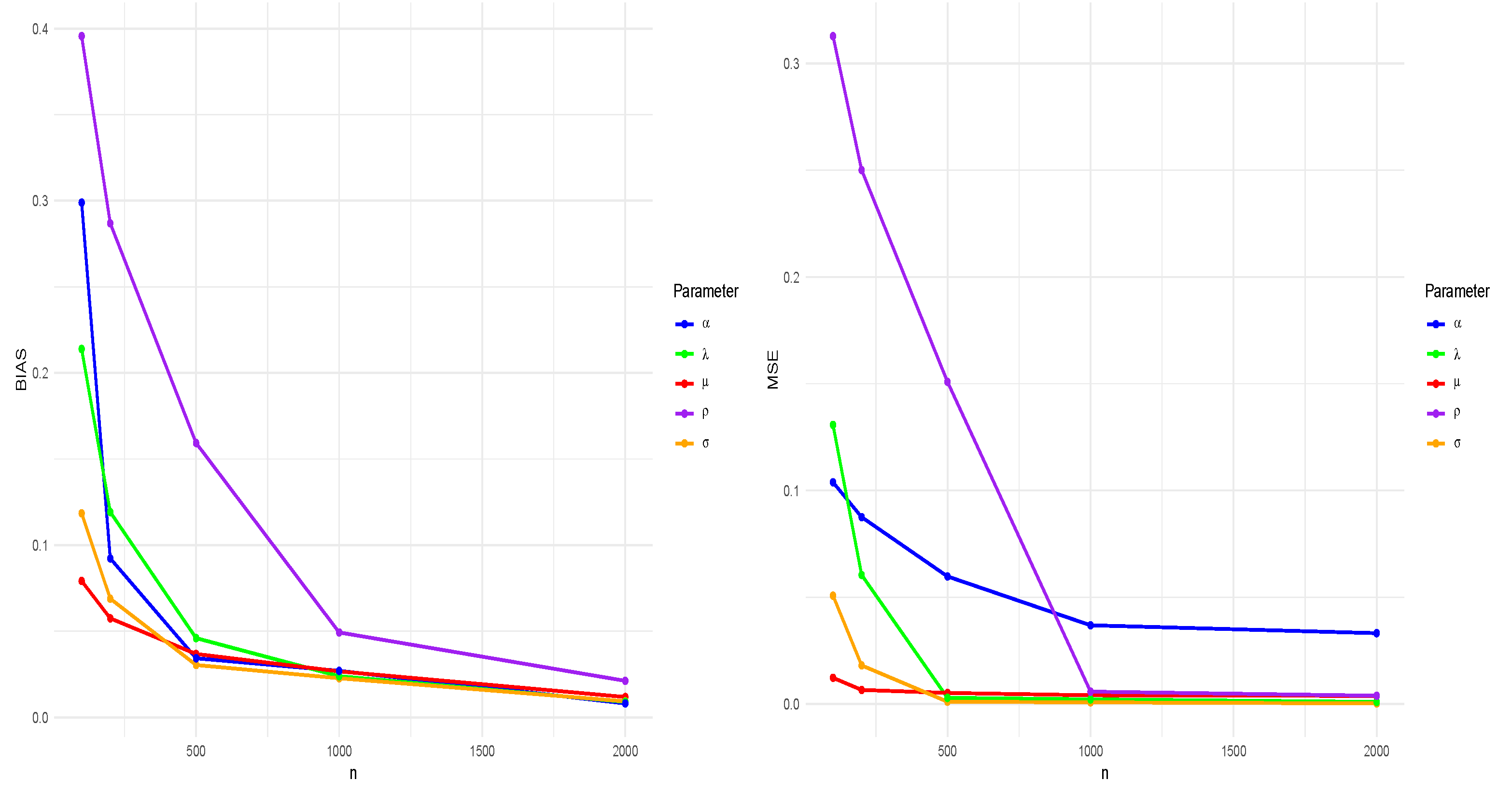
As the evaluation metrics measured for the estimators, the mean squared error (MSE) and bias are computed, and the results are summarized in Table 1. Moreover, Figure 9 shows the MSE of the parameters and the absolute value of bias for different values of n.

Table 1. MLEs and the corresponding biases and MSEs.

n		$\mathit{\mu }$	$\mathit{\sigma }$	$\mathit{\lambda }$	$\mathit{\alpha }$	$\mathit{\rho }$
	Estimate	−0.0792	1.1185	1.2139	0.6989	0.1043
100	Bias	−0.0792	0.1185	0.2139	0.2989	−0.3956
	MSE	0.0122	0.0507	0.1307	0.1038	0.3129
	Estimate	−0.0575	1.0689	1.1192	0.4923	0.2130
200	Bias	−0.0575	0.0689	0.1192	0.0923	−0.2869
	MSE	0.0065	0.0180	0.0604	0.0875	0.2501
	Estimate	0.0368	1.0304	1.0460	0.4343	0.3406
500	Bias	0.0368	0.0304	0.0460	0.0343	−0.1593
	MSE	0.0051	0.0010	0.0028	0.0597	0.1509
	Estimate	−0.0267	1.0227	1.0239	0.4270	0.5493
1000	Bias	−0.0267	0.0227	0.0239	0.0270	0.0493
	MSE	0.0040	0.0007	0.0021	0.0368	0.0057
	Estimate	−0.0118	1.0093	1.0090	0.3918	0.4787
2000	Bias	−0.0118	0.0093	0.0090	−0.0081	−0.0212
	MSE	0.0037	0.0002	0.0008	0.0331	0.0038

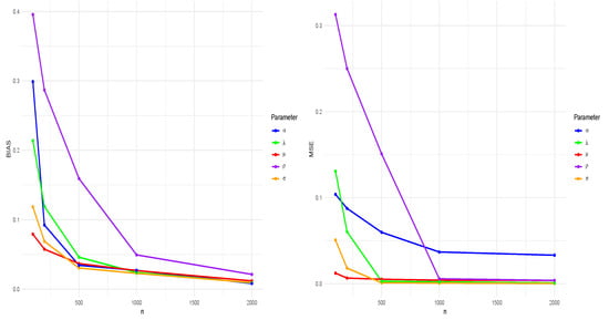
Figure 9. The MSE and absolute bias of the MLEs of the SSGN’s parameters for $\mu =0,\sigma =1,\lambda =1,$$\alpha =0.4,\rho =0.5$, and different values of n.

As it is observed from Figure 9, all of the MLEs are consistent but with different convergence rates. More specifically, the performance of the MLE of $\rho$ for the small and medium sample sizes is not as good as those of other estimators. Therefore, we recommend using the distribution (6) instead of its complementary version in (5) when there is no significant difference in the Akaike information criteria (AICs) of these models for the given real data.

4.2. Real Data Analysis

To demonstrate the practical application of the distributions proposed so far, we examine a real dataset that includes the strength of carbon fibers [18] (see Table 2). Here, we also consider $SN$ and $St$ distributions as the potential competitors of the distributions proposed so far. For fitting these distributions, we respectively employ the functions $\mathtt{sn}.\mathtt{mple}$ and $\mathtt{st}.\mathtt{mple}$, available in the R package $\mathtt{sn}$ [19,20].

Table 2. The strength of carbon fibers [18].

1.901, 2.132, 2.203, 2.228, 2.257, 2.350, 2.361, 2.396, 2.397, 2.445, 2.454, 2.474, 2.518, 2.522, 2.525,

2.532, 2.575, 2.614, 2.616, 2.618, 2.624, 2.659, 2.675, 2.738, 2.740, 2.856, 2.917, 2.928, 2.937, 2.937,

2.977, 2.996, 3.030, 3.125, 3.139, 3.145, 3.220, 3.223, 3.235, 3.243, 3.264, 3.272, 3.294, 3.332, 3.346,

3.377, 3.408, 3.435, 3.493, 3.501, 3.537, 3.554, 3.562, 3.628, 3.852, 3.871, 3.886, 3.971, 4.024, 4.027,

4.225, 4.395, 5.020.

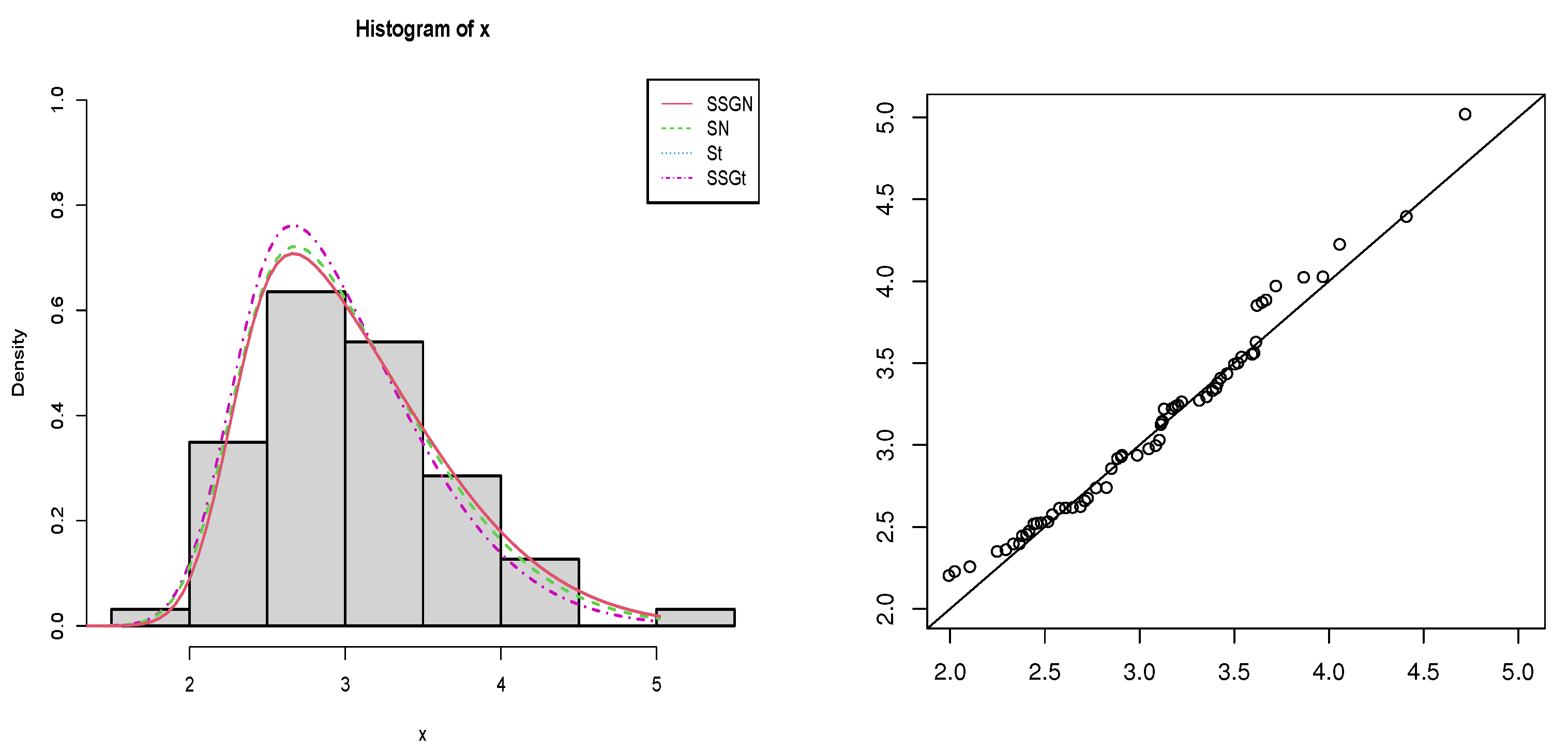
The MLEs of parameters, the corresponding standard error, log-likelihood, Akaike information criterion (AIC), Bayesian Information Criterion (BIC) and the p-value of the Kolmogorov–Smirnov (KS) test are reported in Table 3. According to the p-value of the KS test, the goodness-of-fits of all distributions are confirmed. However, as seen in Table 3, $SSGN$ has the minimum AIC and BIC and thus provides the best fit for the data. The corresponding Q-Q plot of the $SSGN$ model, along with the histogram of the data including the fitted curves, is shown in Figure 10.

Table 3. MLEs (standard errors), log-likelihood, AIC, BIC and p-value of KS test.

Distribution	$\mathbf{SSGN}(\mathit{\mu },\mathit{\sigma },\mathit{\lambda },\mathit{\alpha },\mathit{\rho })$	$\mathbf{SN}(\mathit{\mu },\mathit{\sigma },\mathit{\alpha })$	$\mathbf{St}(\mathit{\mu },\mathit{\sigma },\mathit{\nu },\mathit{\alpha })$	$\mathbf{SSGt}(\mathit{\mu },\mathit{\sigma },\mathit{\nu },\mathit{\lambda },\mathit{\alpha },\mathit{\rho })$
$\widehat{\mu }$	2.2710	2.2709	2.2710	2.2710
	(0.1063)	(0.1667)	(0.1406)	(0.1237)
$\widehat{\sigma }$	1.0005	1.0004	1.0004	1.0004
	(0.0139)	(0.0201)	(0.0110)	(0.0108)
$\widehat{\lambda }$	0.3001	----	----	0.5012
	(0.0109)	----	----	(0.0236)
$\widehat{\alpha }$	4.0018	4.4183	4.4182	3.9862
	(0.0435)	(0.0534)	(0.0547)	(0.0621)
$\widehat{\rho }$	−0.9899	----	----	−0.9899
	(0.0102)	----	----	(0.0184)
$\widehat{\nu }$	----	----	55,897.0701	340.5657
	----	----	(18.0547)	(4.0534)
Log-likelihood	−47.4183	−55.9015	−55.9015	−47.0208
AIC	104.8366	117.8031	119.8033	106.0417
BIC	115.5523	124.2324	128.3755	118.9004
p-value	0.4568	0.8771	0.8765	0.4732

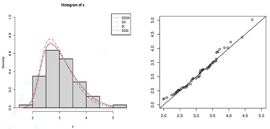
Figure 10. The histogram of the data and the fitted curves (left) and the Q-Q plot of $SSGN$ (right).

The results also indicate that the $SSGt$ distribution provides a good fit for the carbon fiber strength data as evidenced by its AIC value and the p-value from the KS test.

5. Conclusions

In this paper, we introduced the skew-symmetric generalized normal distribution ($SSGN$) and the skew-symmetric generalized t distribution ($SSGt$), extending the framework established by previous studies on skew-normal and skew-t distributions. We derived the density functions, moments, and important statistical properties of these distributions, demonstrating their flexibility in modeling asymmetric data. Moreover, a recurrence relation as well as an exact form for the cdf of the $SSGt$ distribution were obtained. A brief simulation study was also conducted to investigate the behavior of the MLEs of the $SSGN$ parameters. Then, a numerical illustration provided evidence of the practical applicability of the $SSGN$ and $SSGt$ distributions by fitting them to a real dataset concerning the strength of carbon fibers. The results indicated that the $SSGN$ distribution outperformed its competitors, such as the skew-normal and skew-t distributions, in terms of the AIC and the KS test.

References

- Azzalini, A. A class of distributions which includes the normal ones. Scand. J. Stat. 1985, 12, 171–178. [Google Scholar]
- Jamalizadeh, A.; Behboodian, J.; Balakrishnan, N. A two-parameter generalized skew-normal distribution. Stat. Probab. Lett. 2008, 78, 1722–1726. [Google Scholar] [CrossRef]
- Jamalizadeh, A.; Balakrishnan, N. Order statistics from trivariate normal and tν-distributions in terms of generalized skew-normal and skew-tν distributions. J. Stat. Plan. Inference 2009, 139, 3799–3819. [Google Scholar] [CrossRef]
- Arellano-Valle, R.B.; Azzalini, A. On the Unification of Families of Skew-normal Distributions. Scand. J. Stat. 2006, 33, 561–574. [Google Scholar] [CrossRef]
- Azzalini, A.; Capitanio, A. Distributions generated by perturbation of symmetry with emphasis on a multivariate skew-t distribution. J. R. Stat. Soc. Ser. B 2003, 65, 367–389. [Google Scholar] [CrossRef]
- Azzalini, A.; Regoli, G. Some properties of skew-symmetric distributions. Ann. Inst. Stat. Math. 2012, 64, 857–879. [Google Scholar] [CrossRef]
- Nadarajah, S.; Kotz, S. Skewed distributions generated by the normal kernel. Stat. Probab. Lett. 2003, 65, 269–277. [Google Scholar] [CrossRef]
- Gupta, A.K.; Chang, F.C. Multivariate skew-symmetric distributions. Appl. Math. Lett. 2003, 16, 643–646. [Google Scholar] [CrossRef]
- Gomez, H.W.; Venegas, O.; Bolfarine, H. Skew-symmetric distributions generated by the distribution function of the normal distribution. Environmetrics 2007, 18, 395–407. [Google Scholar] [CrossRef]
- Nekoukhou, V.; Alamatsaz, M.H. A family of skew-symmetric-Laplace distributions. Stat. Pap. 2012, 53, 685–696. [Google Scholar] [CrossRef]
- Salehi, M.; Azzalini, A. On application of the univariate Kotz distribution and some of its extensions. METRON 2018, 76, 177–201. [Google Scholar] [CrossRef]
- Salehi, M.; Jamalizadeh, A.; Doostparast, M. A generalized skew two-piece skew-elliptical distribution. Stat. Pap. 2014, 55, 409–429. [Google Scholar] [CrossRef]
- Amiri, M.; Mehrali, Y.; Balakrishnan, N.; Jamalizadeh, A. Efficient recursive computational algorithms for multivariate t and multivariate unified skew-t distributions with applications to inference. Comput. Stat. 2022, 37, 125–158. [Google Scholar] [CrossRef]
- R Core Team. R: A Language and Environment for Statistical Computing; R Foundation for Statistical Computing: Vienna, Austria, 2024; Available online: https://www.R-project.org/ (accessed on 30 September 2024).
- Ardia, D.; Mullen, K.; Peterson, B.; Ulrich, J.; Boudt, K. DEoptim: Global Optimization by Differential Evolution; R 259 Package Version 2.2-5; R Core Team: Vienna, Austria, 2020. [Google Scholar]
- Storn, R.; Price, K. Differential Evolution—A simple and efficient heuristic for global optimization over continuous 292 spaces. J. Glob. Optim. 1997, 11, 341–359. [Google Scholar] [CrossRef]
- Price, K.; Storn, R.M.; Lampinen, J.A. Differential Evolution: A Practical Approach to Global Optimization; Springer Science and Business Media: Berlin/Heidelberg, Germany, 2006. [Google Scholar]
- Badar, M.G.; Priest, A.M. Statistical aspects of fiber and bundle strength in hybrid composites. In Progress in Science and Engineering Composites; Hayashi, T., Kawata, K., Umekawa, S., Eds.; ICCM-IV: Tokyo, Japan, 1982; pp. 1129–1136. [Google Scholar]
- Azzalini, A. The R Package ‘sn’: The Skew-Normal and Related Distributions such as the Skew-t and the SUN (Version 2.1.1). 2023. Available online: http://azzalini.stat.unipd.it/SN/ (accessed on 30 September 2024).
- Azzalini, A.; Salehi, M. Some computational aspects of maximum likelihood estimation of the Skew- distribution. In Computational and Methodological Statistics and Biostatistics; Bekker, A., Chen, G., Ferreira, J., Eds.; Emerging Topics in Statistics and Biostatistics; Springer: Cham, Switzerland, 2020. [Google Scholar] [CrossRef]
Disclaimer/Publisher’s Note: The statements, opinions and data contained in all publications are solely those of the individual author(s) and contributor(s) and not of MDPI and/or the editor(s). MDPI and/or the editor(s) disclaim responsibility for any injury to people or property resulting from any ideas, methods, instructions or products referred to in the content. |
© 2024 by the authors. Licensee MDPI, Basel, Switzerland. This article is an open access article distributed under the terms and conditions of the Creative Commons Attribution (CC BY) license (https://creativecommons.org/licenses/by/4.0/).