Application of Triple- and Quadruple-Generalized Laplace Transform to (2+1)- and (3+1)-Dimensional Time-Fractional Navier–Stokes Equation

Abstract

In this study, the solution of the (2+1)- and (3+1)-dimensional system of the time-fractional Navier–Stokes equations is gained by utilizing the triple-generalized Laplace transform decomposition method (TGLTDM) and quadruple-generalized Laplace transform decomposition method (FGLTDM). In addition, the results of the offered methods match with the exact solutions of the problems, which proves that, as the terms of the series increase, the approximate solutions are closer to the exact solutions of each problem. To verify the appropriateness of these methods, some examples are offered. The TGLTDM and FGLTDM results indicate that the suggested methods have higher evaluation convergence as compared to the ADM and HPM.

1. Introduction

The Navier–Stokes equations are defined as partial differential equations that explain the movement of sticky fluid materials and were first introduced by the researchers in [1]. The Navier–Stokes equation can indicate physical phenomena, fluid flows in conduits and air currents [2,3]. The Navier–Stokes equation is well utilized to deduce the relationship between sticky fluids and solid bodies and is considered the best instrument in the fields of thermohydraulics, meteorology, the petroleum industry, plasma physics, and technology [4]. Various researchers have implemented diverse approaches to gain solutions to the Navier–Stokes equations. For example, the authors in [5] obtained the solution to the time-fractional Navier–Stokes equation by employing a new analytical and approximate method. In [6], the researchers solved the system of time-fractional Navier–Stokes equations by utilizing the hybrid method, which is known as the Laplace Adomian decomposition method.

Numerical results for the multi-dimensional Navier–Stokes equations were acquired using the Adomian decomposition transform method and the q-homotopy analysis transform method [7]. A new recursive transform method, the homotopy perturbation method, with natural transformation, was applied to obtain solutions to the multi-dimensional Navier–Stokes equations [8]. The solution of the fractional multidimensional Navier–Stokes equation with the Caputo fractional derivative operator was examined using the Sumudu transform technique [9].

The combination method known as the variational iteration transform method was applied to solve the fractional-order Navier–Stokes equations [10]. The generalized Laplace transform was initially studied in [11]; additionally, the characteristics of this transformation were examined in [12]. The Laplace-type integral transform connected with the Adomian method was applied to obtain solutions to nonlinear evolution equations endowed with non-integer derivatives [13].

The double-generalized Laplace transform with the decomposition method was applied to gain solutions to the nonlinear sine-Gordon and coupled sine-Gordon equations [14]; later, the same technique was extended to solve a time-fractional partial differential equation [15]. The principal purpose of this study is to find the exact and approximate solutions of multi-dimensional time-fractional Navier–Stokes equations by employing the triple- and quadruple-generalized Laplace decomposition methods.

2. Basic Concepts

In this section, we present some definitions, properties, and theorems for fractional calculus and triple- and quadruple-generalized Laplace transform theory, which are applied in this work.

Definition 1

([11]). Let $f\left(\nu \right)$ be integrable for $\forall \nu \ge 0$. The generalized integral transform $G_{\alpha }$ of the function $f\left(\nu \right)$ is denoted by

$$F\left(s\right)=G_{\alpha }\left(f\right)=s^{\alpha }\underset{0}{\overset{\infty }{\int }}f\left(\nu \right)e^{-{\displaystyle \frac{\nu }{s}}}d\nu ,$$

(1)

for $s\in \mathbb{C}$ and $\alpha \in Z$.

Definition 2.

The Caputo time-fractional derivative operator of order $\alpha >0$ is determined by

$$D_t^{\beta }u(y_1,\nu )=\left\{\begin{array}{c}{\displaystyle \frac{1}{\Gamma \left(m-\alpha \right)}}{\int }_0^{\lambda }{\left(\nu -\lambda \right)}^{m-\alpha -1}{\displaystyle \frac{{\partial }^{m}u(y_1,\tau )}{\partial {\nu }^m}}d\tau ,\\ m-1<\beta <m,\\ {\displaystyle \frac{{\partial }^{m}u(y_1,\nu )}{\partial {\nu }^m}},form=\beta \in \mathbb{N}\end{array}\right.$$

For more details, see [16].

Definition 3

([15]). The triple-generalized Laplace transform (TGLT) of the function $f(y_1,y_2,\nu )$ is defined as

$$\begin{array}{ccc}\hfill F(q_1,q_2,s)& =& G_{y1}{G}_{y_2}{G}_{\nu }\left[f\left(y_1,y_2,\nu \right)\right]\hfill \\ & =& s^{\alpha }{q}_1^{\alpha }{q}_2^{\alpha }\underset{0}{\overset{\infty }{\int }}\underset{0}{\overset{\infty }{\int }}\underset{0}{\overset{\infty }{\int }}{e}^{-({\displaystyle \frac{y_1}{p_1}}+{\displaystyle \frac{y_2}{p_2}}+{\displaystyle \frac{\nu }{s}})}f\left(y_1,y_2,\nu \right)d\nu d{y}_{2}d{y}_1,\hfill \end{array}$$

(2)

where $G_{y_1}{G}_{y_2}{G}_{\nu }$ indicate the TGLT, and the symbols $q_1,q_2$ and s denote transforms of the variables $y_1,y_2$ and ν, respectively.

Definition 4

([15]). The inverse triple-generalized Laplace transform (ITGLT) is

$$\begin{array}{ccc}& & G_{q_1}^{-1}{G}_{q_2}^{-1}{G}_s^{-1}\left(F\left(q_1,q_2,s\right)\right)\hfill \\ & =& f\left(y_1,y_2,t\right)\hfill \\ & =& {\displaystyle \frac{1}{{\left(2\pi i\right)}^3}}{\int }_{\tau -i\infty }^{\tau +i\infty }{\int }_{\varsigma -i\infty }^{\varsigma +i\infty }{\int }_{\eta -i\infty }^{\delta +i\infty }{e}^{{\displaystyle \frac{y_1}{q_1}}+{\displaystyle \frac{y_2}{q_2}}+{\displaystyle \frac{\nu }{s}}}F\left(q_1,q_2,s\right)dsd{q}_{2}d{q}_1,\hfill \end{array}$$

where $G_{q_1}^{-1}{G}_{q_2}^{-1}{G}_s^{-1}$ indicates the IGTLT.

Definition 5.

The quadruple-generalized Laplace transform (FGLT) of the function $f(y_1,y_2,y_3,\nu )$ is defined as

$$\begin{array}{ccc}& & F(q_1,q_2,q_3,s)\hfill \\ & =& G_{y1}{G}_{y_2}{G}_{y_3}{G}_{\nu }\left[f(y_1,y_2,y_3,\nu )\right]\hfill \\ & =& s^{\alpha }{q}_1^{\alpha }{q}_2^{\alpha }{q}_3^{\alpha }\underset{0}{\overset{\infty }{\int }}\underset{0}{\overset{\infty }{\int }}\underset{0}{\overset{\infty }{\int }}\underset{0}{\overset{\infty }{\int }}{e}^{-({\displaystyle \frac{y_1}{q_1}}+{\displaystyle \frac{y_2}{q_2}}+{\displaystyle \frac{y_2}{q_3}}+{\displaystyle \frac{\nu }{s}})}f(y_1,y_2,y_3,\nu )d\nu d{y}_{3}d{y}_{2}d{y}_1,\hfill \end{array}$$

where $G_{y1}{G}_{y_2}{G}_{y_3}{G}_{\nu }$ indicate the FGLT and the symbols $q_1,q_2,q_3$ and s denote transforms of the variables $y_1,y_2,y_3$ and ν, respectively.

Definition 6.

The inverse FGLT is

$$\begin{array}{ccc}& & G_{q_1}^{-1}{G}_{q_2}^{-1}{G}_{q_3}^{-1}{G}_s^{-1}\left(F\left(q_1,q_2,q_3,s\right)\right)\hfill \\ & =& f\left(y_1,y_2,y_3,t\right)\hfill \\ & =& {\displaystyle \frac{1}{{\left(2\pi i\right)}^4}}{\int }_{\tau -i\infty }^{\tau +i\infty }{\int }_{\varsigma -i\infty }^{\varsigma +i\infty }{\int }_{\eta -i\infty }^{\eta +i\infty }{\int }_{\delta -i\infty }^{\delta +i\infty }{\rm Y}dsd{q}_{3}d{q}_{2}d{q}_1,\hfill \end{array}$$

where

$${\rm Y}=e^{{\displaystyle \frac{y_1}{q_1}}+{\displaystyle \frac{y_2}{q_2}}+{\displaystyle \frac{y_3}{q_3}}+{\displaystyle \frac{\nu }{s}}}F\left(q_1,q_2,q_3,s\right),$$

and the symbols $G_{q_1}^{-1}{G}_{q_2}^{-1}{G}_{q_3}^{-1}{G}_s^{-1}$ indicate the IFGLT.

The advantage of the FGLT in generating some transformations from Definition 5 is as follows.

• If we set $\alpha =0$, $s={\displaystyle \frac{1}{s}},q_1={\displaystyle \frac{1}{q_1}},q_2={\displaystyle \frac{1}{q_2}}$ and $q_3={\displaystyle \frac{1}{q_3}}$, we obtain four Laplace transforms:

  $$\begin{array}{ccc}& & L_{y1}{L}_{y_2}{L}_{y_3}{L}_{\nu }\left[f(y_1,y_2,y_3,\nu )\right]\hfill \\ & =& \underset{0}{\overset{\infty }{\int }}\underset{0}{\overset{\infty }{\int }}\underset{0}{\overset{\infty }{\int }}\underset{0}{\overset{\infty }{\int }}f\left(y_1,y_2,y_3,\nu \right)e^{-\left(q_1{y}_1+q_2{y}_2+q_3{y}_3+sv\right)}dvd{y}_{1}d{y}_{2}d{y}_3,\hfill \end{array}$$

  (3)
• If we set $\alpha =0$, $q_1$$={\displaystyle \frac{1}{q_1}}$, $q_2={\displaystyle \frac{1}{q_2}},q_3={\displaystyle \frac{1}{q_3}}$ and substitute s with $\varpi$, we obtain the triple Laplace–Yang transform:

  $$F\left(q_1,q_2,q_3,\varpi \right)=\underset{0}{\overset{\infty }{\int }}\underset{0}{\overset{\infty }{\int }}\underset{0}{\overset{\infty }{\int }}\underset{0}{\overset{\infty }{\int }}f\left(y_1,y_2,y_3,\nu \right)e^{-\left(q_1{y}_1+q_2{y}_2+q_3{y}_3+{\displaystyle \frac{t}{\varpi }}\right)}dvd{y}_{1}d{y}_{2}d{y}_3,$$

  (4)
• At $\alpha =-1$, we obtain the quadruple Sumudu transform:

  $$S_{\chi }{S}_{\gamma }{S}_t\left(f\left(\chi ,\gamma ,t\right)\right)={\displaystyle \frac{1}{q_1{q}_2{q}_{3}s}}\underset{0}{\overset{\infty }{\int }}\underset{0}{\overset{\infty }{\int }}\underset{0}{\overset{\infty }{\int }}\underset{0}{\overset{\infty }{\int }}f\left(y_1,y_2,y_3,\nu \right)e^{-({\displaystyle \frac{y_1}{q_1}}+{\displaystyle \frac{y_2}{q_2}}+{\displaystyle \frac{y_2}{q_3}}+{\displaystyle \frac{\nu }{s}})}dvd{y}_{1}d{y}_{2}d{y}_3.$$

  (5)
  The following notation is used in this work:

  $$\begin{array}{ccc}\hfill G_3& =& G_{y_1}{G}_{y_2}{G}_{\nu },G_3^{-1}=G_{q_1}^{-1}{G}_{q_2}^{-1}{G}_s^{-1}\hfill \\ \hfill G_4& =& G_{y_1}{G}_{y_2}{G}_{y_3}{G}_{\nu },G_4^{-1}=G_{q_1}^{-1}{G}_{q_2}^{-1}{G}_{q_3}^{-1}{G}_s^{-1}.\hfill \end{array}$$

The TGLT of the partial derivatives ${\displaystyle \frac{\partial f(y_1,y_2,\nu )}{\partial y_1}},{\displaystyle \frac{\partial f(y_1,y_2,\nu )}{\partial \nu }}$ and ${\displaystyle \frac{\partial f(y_1,y_2,\nu )}{\partial y_2}}$ is given by

$$\begin{array}{ccc}\hfill G_3\left[{\displaystyle \frac{\partial f(y_1,y_2,\nu )}{\partial y_1}}\right]& =& {\displaystyle \frac{F(q_1,q_2,s)}{q_1}}-q_1^{\alpha }{G}_2\left(f\left(0,y_2,\nu \right)\right),\hfill \\ \hfill G_3\left[{\displaystyle \frac{\partial f(y_1,y_2,\nu )}{\partial y_2}}\right]& =& {\displaystyle \frac{F(q_1,q_2,s)}{q_2}}-q_2^{\alpha }{G}_2\left(f\left(y_1,0,\nu \right)\right),\hfill \\ \hfill G_3\left[{\displaystyle \frac{\partial f(y_1,y_2,\nu )}{\partial \nu }}\right]& =& {\displaystyle \frac{F(q_1,q_2,s)}{s}}-s^{\alpha }{G}_2\left(f\left(y_1,y_2,0\right)\right).\hfill \end{array}$$

Definition 7.

The multi-G-Laplace transform (MGLT) of the function $f\left(y_1,y_2,\dots ,y_n,t\right)$ is offered by

$$\begin{array}{ccc}& & \prod _{j=1}^n{G}_{y_j}{G}_{\nu }\left[f\left(y_1,y_2,\dots ,y_n,\nu \right)\right]\hfill \\ & =& F\left(q_1,q_2,\dots ,q_n,s\right)\hfill \\ & =& s^{\alpha }\prod _{j=1}^n{q}_j^{\alpha }\underset{0}{\overset{\infty }{\int }}\underset{0}{\overset{\infty }{\int }}\dots \underset{0}{\overset{\infty }{\int }}{e}^{-({\displaystyle \frac{y_1}{q_1}}+{\displaystyle \frac{y_2}{q_2}}\dots +{\displaystyle \frac{y_n}{q_n}}+{\displaystyle \frac{\nu }{s}})}f\left(y_1,y_2,\dots ,y_n,\nu \right)d\nu d{y}_{1}d{y}_2\dots d{y}_n,\hfill \end{array}$$

where $j=1,2,3,\dots ,$ so the MGLT of ${\displaystyle \frac{\partial f\left(y_1,y_2,\dots ,y_n,\nu \right)}{\partial \nu }}$ is provided by

$$\begin{array}{ccc}& & \prod _{j=1}^n{G}_{y_j}{G}_{\nu }\left[{\displaystyle \frac{\partial f\left(y_1,y_2,\dots ,y_n,\nu \right)}{\partial \nu }}\right]\hfill \\ & =& {\displaystyle \frac{F\left(q_1,q_2,\dots ,q_n,s\right)}{s^{\beta }}}\hfill \\ & & -s^{\alpha -\beta +1}\prod _{j=1}^n{G}_{y_j}\left[f\left(y_1,y_2,\dots ,y_n,0\right)\right],\hfill \\ \hfill 0& <& \beta \le 1,\hfill \end{array}$$

(6)

In the next theorem, we shall present the FGLT of the partial fractional Caputo derivatives.

Theorem 1.

Let β $>0,$$m-1<\beta \le m$ and $m\in \mathbb{N},$ so that $f\in C^l\left({\mathbb{R}}^{+}\times {\mathbb{R}}^{+}\times {\mathbb{R}}^{+}\times {\mathbb{R}}^{+}\right), l=max\left\{m\right\},$$f^{\left(l\right)}\in L_1\left[\left(0,a\right)\times \left(0,b\right)\times \left(0,c\right)\times \left(0,d\right)\right]$ for any $a,b,c,d$$>0$, $\left|f(y_1,y_2,y_3,\nu )\right|\le K{e}^{y_1{\tau }_1+y_2{\tau }_2+y_3{\tau }_3+\nu {\tau }_4}$, $y_1$$>a>0,y_2>b>0,y_3>c>0$ and $\nu >d>0.$ The quadruple-generalized Laplace transform of Caputo’s fractional derivatives $D_{y_1}^{\beta }\chi (y_1,y_2,y_3,\nu ),$$D_{y_2}^{\beta }\psi (y_1,y_2,y_3,\nu ),D_{y_3}^{\beta }\varphi (y_1,y_2,y_3,\nu )$ and $D_{\nu }^{\beta }\omega (y_1,y_2,y_3,\nu )$ is shown by

$$\begin{array}{ccc}\hfill G_4\left[D_{y_1}^{\beta }\chi (y_1,y_2,y_3,\nu )\right]& =& {\displaystyle \frac{\Theta \left(q_1,q_2,q_3,s\right)}{q_1^{\beta }}}\hfill \\ & & -q_1^{\alpha }\sum _{i=1}^n{\displaystyle \frac{1}{q_1^{\beta -i}}}{G}_{y_2}{G}_{y_3}{G}_{\nu }\left[D_{y_1}^{i-1}\chi \left(0,y_2,y_3,\nu \right)\right],\hfill \\ \hfill n-1& <& \beta <n\hfill \end{array}$$

$$\begin{array}{ccc}\hfill G_4\left[D_{y_2}^{\beta }\psi (y_1,y_2,y_3,\nu )\right]& =& {\displaystyle \frac{\Psi \left(q_1,q_2,q_3,s\right)}{q_2^{\beta }}}\hfill \\ & & -q_2^{\alpha }\sum _{i=1}^n{\displaystyle \frac{1}{q_2^{\beta -i}}}{G}_{y_1}{G}_{y_3}{G}_{\nu }\left[D_{y_2}^{i-1}\psi \left(y_1,0,y_3,\nu \right)\right].\hfill \end{array}$$

$$\begin{array}{ccc}\hfill G_4\left[D_{y_3}^{\beta }\varphi (y_1,y_2,y_3,\nu )\right]& =& {\displaystyle \frac{\Phi \left(q_1,q_2,q_3,s\right)}{q_3^{\beta }}}\hfill \\ & & -q_3^{\alpha }\sum _{i=1}^n{\displaystyle \frac{1}{q_3^{\beta -i}}}{G}_{y_1}{G}_{y_2}{G}_{\nu }\left[D_{y_3}^{i-1}\varphi \left(y_1,y_2,0,\nu \right)\right].\hfill \end{array}$$

and

$$\begin{array}{ccc}\hfill G_4\left[D_{\nu }^{\beta }\omega (y_1,y_2,y_3,\nu )\right]& =& {\displaystyle \frac{ϝ\left(q_1,q_2,q_3,s\right)}{s^{\beta }}}\hfill \\ & & -s^{\alpha }\sum _{i=1}^n{\displaystyle \frac{1}{s^{\beta -i}}}{G}_{y_1}{G}_{y_2}{G}_{y_3}\left[D_{\nu }^{i-1}\omega \left(y_1,y_2,y_3,0\right)\right].\hfill \end{array}$$

The following steps describe the triple-generalized Laplace transform decomposition method.

• Taking the triple-generalized Laplace transform for the (2+1)-dimensional time-fractional Navier–Stokes equations;
• Applying the double-generalized Laplace transformation for the initial conditions;
• Using the inverse TGLT for the obtained equation;
• Applying a decomposed infinite series as a solution to the (2+1)-dimensional time-fractional Navier–Stokes equations.

3. Explanation of the Method of the Triple-Generalized Laplace Transform Decomposition Method (TGLTDM)

In this section of the work, we give the essential concept of the triple-generalized Laplace transform decomposition method (TGLTDM) for the FPDEs. To demonstrate the basic plan of the TGLTDM, we consider the following (2+1)-dimensional time-fractional Navier–Stokes equations:

$$\begin{array}{ccc}\hfill D_{\nu }^{\beta }\chi +\chi {\displaystyle \frac{\partial \chi }{\partial y_1}}+\omega {\displaystyle \frac{\partial \chi }{\partial y_2}}& =& k\left({\displaystyle \frac{{\partial }^2\chi }{\partial y_1^2}}+{\displaystyle \frac{{\partial }^2\chi }{\partial y_2^2}}\right)-{\displaystyle \frac{1}{\rho }}{\displaystyle \frac{\partial p}{\partial y_1}},\hfill \\ \hfill D_{\nu }^{\beta }\omega +\chi {\displaystyle \frac{\partial \omega }{\partial y_1}}+\omega {\displaystyle \frac{\partial \omega }{\partial y_2}}& =& k\left({\displaystyle \frac{{\partial }^2\omega }{\partial y_1^2}}+{\displaystyle \frac{{\partial }^2\omega }{\partial y_2^2}}\right)-{\displaystyle \frac{1}{\rho }}{\displaystyle \frac{\partial p}{\partial y_2}},\hfill \\ \hfill y_1,y_2,t& >& 0,n-1<\beta <n;\hfill \end{array}$$

(7)

with the initial conditions

$$\chi (y_1,y_2,0)=f_1(y_1,y_2),\omega (y_1,y_2,0)=f_2(y_1,y_2)$$

(8)

where $D_{\nu }^{\beta }={\displaystyle \frac{{\partial }^{\beta }}{\partial t^{\beta }}}$ is the fractional Caputo derivative; $k={\displaystyle \frac{\mu }{\rho }}$ is defined as the kinematic viscosity of the flow; $\mu$ denotes the dynamic viscosity; and $\rho$ is the density if p is known; then, $p_1=$${\displaystyle \frac{1}{\rho }}{\displaystyle \frac{\partial p}{\partial x}}$ and $p_2=-{\displaystyle \frac{1}{\rho }}{\displaystyle \frac{\partial p}{\partial y}}.$ To gain a solution to Equation (7), the following steps are needed.

• Applying the TGLT for Equation (7), one can obtain

$$\begin{array}{ccc}\hfill {\displaystyle \frac{G_3\left[\chi (y_1,y_2,\nu )\right]}{s^{\beta }}}& =& s^{\alpha -\beta +1}{G}_2\left(\chi (y_1,y_2,0)\right)-G_3\left(\chi {\displaystyle \frac{\partial \chi }{\partial y_1}}+\omega {\displaystyle \frac{\partial \chi }{\partial y_2}}\right)\hfill \\ & & +G_3\left(k\left({\displaystyle \frac{{\partial }^2\chi }{\partial y_1^2}}+{\displaystyle \frac{{\partial }^2\chi }{\partial y_2^2}}\right)\right)-G_3\left(p_1\right),\hfill \\ \hfill {\displaystyle \frac{G_3\left[\omega (y_1,y_2,\nu )\right]}{s^{\beta }}}& =& s^{\alpha -\beta +1}{G}_2\left(\omega (y_1,y_2,0)\right)-G_3\left(\chi {\displaystyle \frac{\partial \omega }{\partial y_1}}+\omega {\displaystyle \frac{\partial \omega }{\partial y_2}}\right)\hfill \\ & & +G_3\left(k\left({\displaystyle \frac{{\partial }^2\omega }{\partial y_1^2}}+{\displaystyle \frac{{\partial }^2\omega }{\partial y_2^2}}\right)\right)+G_3\left(p_2\right),\hfill \end{array}$$

(9)

2.

Now, taking the DGLT for Equation (8) and substituting it in Equation (9), we have

$$\begin{array}{ccc}\hfill \Theta \left(q_1,q_2,s\right)& =& s^{\alpha +1}{F}_1\left(q_1,q_2\right)-s^{\beta }{G}_3\left(\chi {\displaystyle \frac{\partial \chi }{\partial y_1}}+\omega {\displaystyle \frac{\partial \chi }{\partial y_2}}\right)\hfill \\ & & +s^{\beta }{G}_3\left(k\left({\displaystyle \frac{{\partial }^2\chi }{\partial y_1^2}}+{\displaystyle \frac{{\partial }^2\chi }{\partial y_2^2}}\right)\right)-s^{\beta }{G}_3\left(p_1\right),\hfill \\ \hfill \Psi \left(q_1,q_2,s\right)& =& s^{\alpha +1}{F}_2\left(q_1,q_2\right)-s^{\beta }{G}_3\left(\chi {\displaystyle \frac{\partial \omega }{\partial y_1}}+\omega {\displaystyle \frac{\partial \omega }{\partial y_2}}\right)\hfill \\ & & +s^{\beta }{G}_3\left(k\left({\displaystyle \frac{{\partial }^2\omega }{\partial y_1^2}}+{\displaystyle \frac{{\partial }^2\omega }{\partial y_2^2}}\right)\right)+s^{\beta }{G}_3\left(p_2\right),\hfill \end{array}$$

(10)

3.

On using the inverse TGLT for Equation (10), we have

$$\begin{array}{ccc}\hfill \chi (y_1,y_2,\nu )& =& G_3^{-1}\left(s^{\alpha +1}{F}_1\left(q_1,q_2\right)-s^{\beta }{G}_3\left(p_1\right)\right)\hfill \\ & & -G_3^{-1}\left(s^{\beta }{G}_3\left(\chi {\displaystyle \frac{\partial \chi }{\partial y_1}}+\omega {\displaystyle \frac{\partial \chi }{\partial y_2}}\right)\right)\hfill \\ & & +G_3^{-1}\left(s^{\beta }{G}_3\left(k\left({\displaystyle \frac{{\partial }^2\chi }{\partial y_1^2}}+{\displaystyle \frac{{\partial }^2\chi }{\partial y_2^2}}\right)\right)\right)\hfill \end{array}$$

(11)

and

$$\begin{array}{ccc}\hfill \omega (y_1,y_2,\nu )& =& G_3^{-1}\left(s^{\alpha +1}{F}_2\left(q_1,q_2\right)+s^{\beta }{G}_3\left(p_1\right)\right)\hfill \\ & & -G_3^{-1}\left(s^{\beta }{G}_3\left(\chi {\displaystyle \frac{\partial \omega }{\partial y_1}}+\omega {\displaystyle \frac{\partial \omega }{\partial y_2}}\right)\right)\hfill \\ & & +G_3^{-1}\left(s^{\beta }{G}_3\left(k\left({\displaystyle \frac{{\partial }^2\omega }{\partial y_1^2}}+{\displaystyle \frac{{\partial }^2\omega }{\partial y_2^2}}\right)\right)\right).\hfill \end{array}$$

(12)

4.

The TGLTDM solutions $\chi (y_1,y_2,\nu )$ and $\omega (y_1,y_2,\nu )$ are offered by the following infinite series:

$$\begin{array}{ccc}\hfill \chi (y_1,y_2,\nu )& =& \sum _{n=0}^{\infty }{\chi }_n(y_1,y_2,\nu ),\hfill \\ \hfill \omega (y_1,y_2,\nu )& =& \sum _{n=0}^{\infty }{\omega }_n(y_1,y_2,\nu ),\hfill \end{array}$$

(13)

and therefore the nonlinear terms $\chi {\displaystyle \frac{\partial \chi }{\partial y_1}},\omega {\displaystyle \frac{\partial \chi }{\partial y_2}},\chi {\displaystyle \frac{\partial \omega }{\partial y_1}}$ and $\omega {\displaystyle \frac{\partial \omega }{\partial y_2}}$ are fixed by

$$\begin{array}{ccc}\hfill \chi {\displaystyle \frac{\partial \chi }{\partial y_1}}& =& \sum _{n=0}^{\infty }{A}_n,\omega {\displaystyle \frac{\partial \chi }{\partial y_2}}=\sum _{n=0}^{\infty }{B}_n,\hfill \\ \hfill \chi {\displaystyle \frac{\partial \omega }{\partial y_1}}& =& \sum _{n=0}^{\infty }{C}_n,\omega {\displaystyle \frac{\partial \omega }{\partial y_2}}=\sum _{n=0}^{\infty }{D}_n.\hfill \end{array}$$

(14)

5.

By substituting Equations (13) and (14) into Equations (11) and (12), one can obtain

$$\begin{array}{ccc}\hfill \sum _{n=0}^{\infty }{\chi }_n(y_1,y_2,\nu )& =& G_3^{-1}\left(s^{\alpha +1}{F}_1\left(q_1,q_2\right)-s^{\beta }{G}_3\left(p_1\right)\right)\hfill \\ & & -G_3^{-1}\left(s^{\beta }{G}_3\left(\chi \sum _{n=0}^{\infty }\left(A_n+B_n\right)\right)\right)\hfill \\ & & +G_3^{-1}\left(s^{\beta }{G}_3\left(k\left(\sum _{n=0}^{\infty }\left({\displaystyle \frac{{\partial }^2{\chi }_n}{\partial y_1^2}}+{\displaystyle \frac{{\partial }^2{\chi }_n}{\partial y_2^2}}\right)\right)\right)\right),\hfill \end{array}$$

and

$$\begin{array}{ccc}\hfill \sum _{n=0}^{\infty }{\omega }_n(y_1,y_2,\nu )& =& G_3^{-1}\left(s^{\alpha +1}{F}_2\left(q_1,q_2\right)+s^{\beta }{G}_3\left(p_1\right)\right)\hfill \\ & & -G_3^{-1}\left(s^{\beta }{G}_3\left(\sum _{n=0}^{\infty }{C}_n+D_n\right)\right)\hfill \\ & & +G_3^{-1}\left(s^{\beta }{G}_3\left(k\left(\sum _{n=0}^{\infty }\left({\displaystyle \frac{{\partial }^2{\omega }_n}{\partial y_1^2}}+{\displaystyle \frac{{\partial }^2{\omega }_n}{\partial y_2^2}}\right)\right)\right)\right).\hfill \end{array}$$

We establish the repeated relationship for the above equations by exploiting the decomposition method, and we will obtain

$$\begin{array}{ccc}\hfill {\chi }_0(y_1,y_2,\nu )& =& G_3^{-1}\left(s^{\alpha +1}{F}_1\left(q_1,q_2\right)-s^{\beta }{G}_3\left(p_1\right)\right),\hfill \\ \hfill {\omega }_0(y_1,y_2,\nu )& =& G_3^{-1}\left(s^{\alpha +1}{F}_2\left(q_1,q_2\right)+s^{\beta }{G}_3\left(p_1\right)\right),\hfill \end{array}$$

(15)

and the remainder of the components ${\chi }_{n+1}$ and ${\omega }_{n+1},n\ge 0$ are granted by

$$\begin{array}{ccc}\hfill {\chi }_{n+1}(y_1,y_2,\nu )& =& -G_3^{-1}\left(s^{\beta }{G}_3\left(A_n+B_n\right)\right)\hfill \\ & & +G_3^{-1}\left(s^{\beta }{G}_3\left(k\left({\displaystyle \frac{{\partial }^2{\chi }_n}{\partial y_1^2}}+{\displaystyle \frac{{\partial }^2{\chi }_n}{\partial y_2^2}}\right)\right)\right),\hfill \end{array}$$

(16)

and

$$\begin{array}{ccc}\hfill {\omega }_{n+1}(y_1,y_2,\nu )& =& -G_3^{-1}\left(s^{\beta }{G}_3\left(C_n+D_n\right)\right)\hfill \\ & & +G_3^{-1}\left(s^{\beta }{G}_3\left(k\left({\displaystyle \frac{{\partial }^2{\omega }_n}{\partial y_1^2}}+{\displaystyle \frac{{\partial }^2{\omega }_n}{\partial y_2^2}}\right)\right)\right),\hfill \end{array}$$

(17)

where $G_3$ indicates the TGLT with respect to $y_1,y_2,\nu$ and the ITGLT is denoted by $G_3^{-1}$ with respect to $q_1,q_2,s$. We find that the ITGLT with respect to $q_1,q_2$ and s exists for Equations (15)–(17).

Example 1.

Consider the (2+1)-dimensional time-fractional Navier–Stokes equation

$$\begin{array}{ccc}\hfill D_t^{\alpha }\chi +\chi {\chi }_{y_1}+\omega {\chi }_{y_2}& =& k\left({\chi }_{y_1{y}_1}+{\chi }_{y_2{y}_2}\right)+p_1,y_1,y_2,\nu >0,\hfill \\ \hfill D_t^{\alpha }\omega +\chi {\omega }_{y_1}+\omega {\omega }_{y_2}& =& k\left({\omega }_{y_1{y}_1}+{\omega }_{y_2{y}_2}\right)-p_2,y_1,y_2,\nu >0,\hfill \\ \hfill n-1& <& \alpha <n;\hfill \end{array}$$

(18)

subject to the conditions

$$\begin{array}{ccc}\hfill \chi (y_1,y_2,0)& =& -exp(y_1+y_2),\hfill \\ \hfill \omega (y_1,y_2,0)& =& exp(y_1+y_2)\hfill \end{array}$$

(19)

By using the TGLT on both sides of Equation (18), we obtain

$$\begin{array}{ccc}& & G_3\left[D_t^{\alpha }\chi +\chi {\chi }_x+\omega {\chi }_y=k\left({\chi }_{xx}+{\chi }_{yy}\right)+p_1\right]\hfill \\ & & G_3\left[D_t^{\alpha }\omega +\chi {\omega }_x+\omega {\omega }_y=k\left({\omega }_{xx}+{\omega }_{yy}\right)-p_2\right],\hfill \end{array}$$

(20)

and applying the DGLT for Equation (19) and substituting it in Equation (20), we acquire

$$\begin{array}{ccc}\hfill \Theta \left(q_1,q_2,s\right)& =& -s^{\alpha +1}{\displaystyle \frac{q_1^{\alpha +1}}{1-q_1}}{\displaystyle \frac{q_2^{\alpha +1}}{1-q_2}}\hfill \\ & & -s^{\beta }{G}_3\left(\chi {\displaystyle \frac{\partial \chi }{\partial y_1}}+\omega {\displaystyle \frac{\partial \chi }{\partial y_2}}\right)\hfill \\ & & +s^{\beta }{G}_3\left(k\left({\displaystyle \frac{{\partial }^2\chi }{\partial y_1^2}}+{\displaystyle \frac{{\partial }^2\chi }{\partial y_2^2}}\right)\right)+s^{\beta }{G}_3\left(p_1\right),\hfill \\ \hfill \Psi \left(q_1,q_2,s\right)& =& s^{\alpha +1}{\displaystyle \frac{q_1^{\alpha +1}}{1-q_1}}{\displaystyle \frac{q_2^{\alpha +1}}{1-q_2}}\hfill \\ & & -s^{\beta }{G}_3\left(\chi {\displaystyle \frac{\partial \omega }{\partial y_1}}+\omega {\displaystyle \frac{\partial \omega }{\partial y_2}}\right)\hfill \\ & & +s^{\beta }{G}_3\left(k\left({\displaystyle \frac{{\partial }^2\omega }{\partial y_1^2}}+{\displaystyle \frac{{\partial }^2\omega }{\partial y_2^2}}\right)\right)-s^{\beta }{G}_3\left(p_2\right),\hfill \end{array}$$

(21)

Now, implementing the ITGLT for Equation (21), we have

$$\begin{array}{ccc}\hfill \chi (y_1,y_2,\nu )& =& -exp(y_1+y_2)+{\displaystyle \frac{p_1{\nu }^{\beta }}{\Gamma \left(\beta +1\right)}}\hfill \\ & & -G_3^{-1}\left(s^{\beta }{G}_3\left(\chi {\displaystyle \frac{\partial \chi }{\partial y_1}}+\omega {\displaystyle \frac{\partial \chi }{\partial y_2}}\right)\right)\hfill \\ & & +G_3^{-1}\left(s^{\beta }{G}_3\left(k\left({\displaystyle \frac{{\partial }^2\chi }{\partial y_1^2}}+{\displaystyle \frac{{\partial }^2\chi }{\partial y_2^2}}\right)\right)\right),\hfill \\ \hfill \omega (y_1,y_2,\nu )& =& exp(x+y)-{\displaystyle \frac{p_2{\nu }^{\beta }}{\Gamma \left(\beta +1\right)}}\hfill \\ & & -G_3^{-1}\left(s^{\beta }{G}_3\left(\chi {\displaystyle \frac{\partial \omega }{\partial y_1}}+\omega {\displaystyle \frac{\partial \omega }{\partial y_2}}\right)\right)\hfill \\ & & +G_3^{-1}\left(s^{\beta }{G}_3\left(k\left({\displaystyle \frac{{\partial }^2\omega }{\partial y_1^2}}+{\displaystyle \frac{{\partial }^2\omega }{\partial y_2^2}}\right)\right)\right).\hfill \end{array}$$

(22)

The zeroth components ${\chi }_0$ and ${\omega }_0$ are suggested by the decomposition method, which constantly includes the initial conditions and the source term, which are supposed to be familiar. Consequently, we let

$$\begin{array}{ccc}\hfill {\chi }_0& =& -exp(x+y)+{\displaystyle \frac{p_1{\nu }^{\beta }}{\Gamma \left(\beta +1\right)}},\hfill \\ \hfill {\omega }_0& =& sin(x+y)-{\displaystyle \frac{p_2{\nu }^{\beta }}{\Gamma \left(\beta +1\right)}},\hfill \end{array}$$

The remaining components ${\chi }_{n+1}$, ${\omega }_{n+1},$ $n\ge 0$ are denoted by applying the following relations:

$$\begin{array}{ccc}\hfill {\chi }_{n+1}& =& -G_3^{-1}\left(s^{\beta }{G}_3\left(\left(A_n+B_n\right)\right)\right)\hfill \\ & & +G_3^{-1}\left(s^{\beta }{G}_3\left(k\left({\chi }_{nxx}+{\chi }_{nyy}\right)\right)\right),\hfill \end{array}$$

(23)

and

$$\begin{array}{ccc}\hfill {\omega }_{n+1}& =& -G_3^{-1}\left(s^{\beta }{G}_3\left(C_n+D_n\right)\right)\hfill \\ & & +G_3^{-1}\left(s^{\beta }{G}_3\left(k\left({\omega }_{nxx}+{\omega }_{nyy}\right)\right)\right)\hfill \end{array}$$

(24)

The few terms of the Adomian polynomials $A_n, B_n$, $C_n$ and $D_n$ are defined by

$$\begin{array}{ccc}\hfill A_0& =& {\chi }_0{\chi }_{0y_1},A_1={\chi }_0{\chi }_{1y_1}+{\chi }_1{\chi }_{0y_1},\hfill \\ \hfill A_2& =& {\chi }_0{\chi }_{2y_1}+{\chi }_1{\chi }_{1y_1}+{\chi }_2{\chi }_{0y_1},\hfill \\ \hfill A_3& =& {\chi }_0{\chi }_{3y_1}+{\chi }_1{\chi }_{2y_1}+{\chi }_2{\chi }_{1y_1}+{\chi }_3{\chi }_{0y_1},\hfill \end{array}$$

(25)

$$\begin{array}{ccc}\hfill B_0& =& {\omega }_0{\chi }_{0y_2},B_1={\omega }_0{\chi }_{1y_2}+{\omega }_1{\chi }_{0y_2},\hfill \\ \hfill B_2& =& {\omega }_0{\chi }_{2y_2}+{\omega }_1{\chi }_{1y_2}+{\omega }_2{\chi }_{0y_2},\hfill \\ \hfill B_3& =& {\omega }_0{\chi }_{3y_2}+{\omega }_1{\chi }_{2y_2}+{\omega }_2{\chi }_{1y_2}+{\omega }_3{\chi }_{0y_2},\hfill \end{array}$$

(26)

$$\begin{array}{ccc}\hfill C_0& =& {\chi }_0{\omega }_{0y_1},C_1={\chi }_0{\omega }_{1y_1}+{\chi }_1{\omega }_{0y_1},\hfill \\ \hfill C_2& =& {\chi }_0{\omega }_{2y_1}+{\chi }_1{\omega }_{1y_1}+{\chi }_2{\omega }_{0y_1},\hfill \\ \hfill C_3& =& {\chi }_0{\omega }_{3y_1}+{\chi }_1{\omega }_{2y_1}+{\chi }_2{\omega }_{1y_1}+{\chi }_3{\omega }_{0y_1}.\hfill \end{array}$$

(27)

$$\begin{array}{ccc}\hfill D_0& =& {\omega }_0{\omega }_{0y_2},D_1={\omega }_0{\omega }_{1y_2}+{\omega }_1{\omega }_{0y_2},\hfill \\ \hfill D_2& =& {\omega }_0{\omega }_{2y_2}+{\omega }_1{\omega }_{1y_2}+{\omega }_2{\omega }_{2y_2},\hfill \\ \hfill D_3& =& {\omega }_0{\omega }_{3y_2}+{\omega }_1{\omega }_{2y_2}+{\omega }_2{\omega }_{1y_2}+{\omega }_3{\omega }_{0y_2}.\hfill \end{array}$$

(28)

By putting $n=0$ into Equations (23) and (24), we gain

$$\begin{array}{ccc}\hfill {\chi }_1& =& -G_3^{-1}\left(s^{\beta }{G}_3\left(\left(A_0+B_0\right)\right)\right)\hfill \\ & & +G_3^{-1}\left(s^{\beta }{G}_3\left(k\left({\chi }_{0xx}+{\chi }_{0yy}\right)\right)\right)\hfill \\ & =& G_3^{-1}\left(s^{\beta }{G}_3\left(-2kexp(y_1+y_2)\right)\right)\hfill \\ & =& G_3^{-1}\left[{\displaystyle \frac{-2k{q}_1^{\alpha +1}{q}_2^{\alpha +1}{s}^{\alpha +\beta +1}}{\left(1-q_1\right)\left(1-q_2\right)}}\right]\hfill \\ & =& -2kexp(y_1+y_2){\displaystyle \frac{{\nu }^{\beta }}{\Gamma \left(\beta +1\right)}},\hfill \end{array}$$

and

$$\begin{array}{ccc}\hfill {\omega }_1& =& -G_3^{-1}\left(s^{\beta }{G}_3\left(C_0+D_0\right)\right)\hfill \\ & & +G_3^{-1}\left(s^{\beta }{G}_3\left(k\left({\omega }_{0xx}+{\omega }_{0yy}\right)\right)\right)\hfill \\ & =& G_3^{-1}\left(s^{\beta }{G}_3\left(2kexp(y_1+y_2)\right)\right)\hfill \\ & =& G_3^{-1}\left[{\displaystyle \frac{2k{q}_1^{\alpha +1}{q}_2^{\alpha +1}{s}^{\alpha +\beta +1}}{\left(1-q_1\right)\left(1-q_2\right)}}\right]\hfill \\ & =& 2kexp(y_1+y_2){\displaystyle \frac{{\nu }^{\beta }}{\Gamma \left(\beta +1\right)}},\hfill \end{array}$$

and, similarly, at $n=1,$

$$\begin{array}{ccc}\hfill {\chi }_2& =& -G_3^{-1}\left(s^{\beta }{G}_3\left(\left({\chi }_0{\chi }_{1x}+{\chi }_1{\chi }_{0x}+{\omega }_0{\chi }_{1y}+{\omega }_1{\chi }_{0y}\right)\right)\right)\hfill \\ & & +G_3^{-1}\left(s^{\beta }{G}_3\left(k\left({\chi }_{1xx}+{\chi }_{1yy}\right)\right)\right),\hfill \\ & =& G_3^{-1}\left(s^{\beta }{G}_3\left(-4k^{2}exp(y_1+y_2){\displaystyle \frac{{\nu }^{\beta }}{\Gamma \left(\beta +1\right)}}\right)\right)\hfill \\ & =& G_3^{-1}\left(-4k^2{\displaystyle \frac{q_1^{\alpha +1}{q}_2^{\alpha +1}{s}^{\alpha +2\beta +1}}{\left(1-q_1\right)\left(1-q_2\right)}}\right)\hfill \\ \hfill {\chi }_2& =& -4k^{2}exp(y_1+y_2){\displaystyle \frac{{\nu }^{2\beta }}{\Gamma \left(2\beta +1\right)}},\hfill \end{array}$$

and

$$\begin{array}{ccc}\hfill {\omega }_2& =& -G_3^{-1}\left(s^{\beta }{G}_3\left({\chi }_0{\omega }_{1x}+{\chi }_1{\omega }_{0x}+{\omega }_0{\omega }_{1y}+{\omega }_1{\omega }_{0y}\right)\right)\hfill \\ & & +G_3^{-1}\left(s^{\beta }{G}_3\left(k\left({\omega }_{0xx}+{\omega }_{0yy}\right)\right)\right)\hfill \\ & =& G_3^{-1}\left(s^{\beta }{G}_3\left(4k^{2}exp(y_1+y_2){\displaystyle \frac{{\nu }^{\beta }}{\Gamma \left(\beta +1\right)}}\right)\right)\hfill \\ & =& G_3^{-1}\left(4k^2{\displaystyle \frac{q_1^{\alpha +1}{q}_2^{\alpha +1}{s}^{\alpha +2\beta +1}}{\left(1-q_1\right)\left(1-q_2\right)}}\right)\hfill \\ & =& 4k^{2}exp(y_1+y_2){\displaystyle \frac{{\nu }^{2\beta }}{\Gamma \left(2\beta +1\right)}},\hfill \end{array}$$

while, at $n=2,$ we have

$$\begin{array}{ccc}\hfill {\chi }_3& =& -G_3^{-1}\left(s^{\beta }{G}_3\left(\left(\begin{array}{c}{\chi }_0{\chi }_{2x}+{\chi }_1{\chi }_{1x}+{\chi }_2{\chi }_{0x}\\ +{\omega }_0{\chi }_{2y}+{\omega }_1{\chi }_{1y}+{\omega }_2{\chi }_{0y}\end{array}\right)\right)\right)\hfill \\ & & +G_3^{-1}\left(s^{\beta }{G}_3\left(k\left({\chi }_{2xx}+{\chi }_{2yy}\right)\right)\right),\hfill \\ & =& G_3^{-1}\left(s^{\beta }{G}_3\left(-8k^{3}exp(y_1+y_2){\displaystyle \frac{{\nu }^{2\beta }}{\Gamma \left(2\beta +1\right)}}\right)\right)\hfill \\ & =& G_3^{-1}\left(-8k^3{\displaystyle \frac{q_1^{\alpha +1}{q}_2^{\alpha +1}{s}^{\alpha +3\beta +1}}{\left(1-q_1\right)\left(1-q_2\right)}}\right)\hfill \\ \hfill {\chi }_3& =& -8k^{3}exp(y_1+y_2){\displaystyle \frac{{\nu }^{3\beta }}{\Gamma \left(3\beta +1\right)}},\hfill \end{array}$$

and

$$\begin{array}{ccc}\hfill {\omega }_3& =& -G_3^{-1}\left(s^{\beta }{G}_3\left(\begin{array}{c}{\chi }_0{\omega }_{2x}+{\chi }_1{\omega }_{1x}+{\chi }_2{\omega }_{0x}\\ +{\omega }_0{\omega }_{2y}+{\omega }_1{\omega }_{1y}+{\omega }_2{\omega }_{2y}\end{array}\right)\right)\hfill \\ & & +G_3^{-1}\left(s^{\beta }{G}_3\left(k\left({\omega }_{0xx}+{\omega }_{0yy}\right)\right)\right)\hfill \\ & =& G_3^{-1}\left(s^{\beta }{G}_3\left(8k^{3}exp(y_1+y_2){\displaystyle \frac{{\nu }^{2\beta }}{\Gamma \left(2\beta +1\right)}}\right)\right)\hfill \\ & =& G_3^{-1}\left(8k^3{\displaystyle \frac{q_1^{\alpha +1}{q}_2^{\alpha +1}{s}^{\alpha +3\beta +1}}{\left(1-q_1\right)\left(1-q_2\right)}}\right)\hfill \\ & =& 8k^{3}exp(y_1+y_2){\displaystyle \frac{{\nu }^{3\beta }}{\Gamma \left(3\beta +1\right)}}.\hfill \end{array}$$

In the same way, we have

$${\chi }_n=-{\left(2k\right)}^{n}exp(y_1+y_2){\displaystyle \frac{{\nu }^{n\beta }}{\Gamma \left(n\beta +1\right)}},{\omega }_n={\left(2k\right)}^{n}exp(y_1+y_2){\displaystyle \frac{{\nu }^{n\beta }}{\Gamma \left(n\beta +1\right)}},\forall n\ge 2.$$

The solution of Equation (18) is denoted by

$$\begin{array}{ccc}\hfill \chi (y_1,y_2,\nu )& =& {\chi }_0+{\chi }_1+{\chi }_2+\dots +{\chi }_n\hfill \\ \hfill \omega (y_1,y_2,\nu )& =& {\omega }_0+{\omega }_1+{\omega }_2+\dots +{\omega }_n,\hfill \end{array}$$

therefore,

$$\begin{array}{ccc}\hfill \chi (y_1,y_2,\nu )& =& -exp(y_1+y_2)\sum _{n=1}^{\infty }{\displaystyle \frac{{\left(2k\right)}^n{t}^{n\beta }}{\Gamma \left(n\beta +1\right)}}+{\displaystyle \frac{p_1{t}^{\beta }}{\Gamma \left(\beta +1\right)}},\hfill \\ \hfill \omega (y_1,y_2,\nu )& =& exp(y_1+y_2)\sum _{n=1}^{\infty }{\displaystyle \frac{{\left(2k\right)}^n{t}^{n\beta }}{\Gamma \left(n\beta +1\right)}}-{\displaystyle \frac{p_2{t}^{\beta }}{\Gamma \left(\beta +1\right)}}.\hfill \end{array}$$

In particular, at $\beta =1$ and $p_1=p_2=0,$ we obtain the exact solution of the classical Navier–Stokes equation for the velocity as

$$\begin{array}{ccc}\hfill \chi (y_1,y_2,\nu )& =& -exp(y_1+y_2-2k\nu ),\hfill \\ \hfill \omega (y_1,y_2,\nu )& =& exp(y_1+y_2+2k\nu ).\hfill \end{array}$$

The results obtained agree with [7].

4. Analysis of the Quadruple-Generalized Laplace Transform Decomposition Method (FGLTDM)

In this section, we establish an approximate analytical solution for the (3+1)-dimensional time-fractional Navier–Stokes equations by utilizing the FGLTDM.

Consider that the (3+1) time-fractional model of the Navier–Stokes equation is given by

$$\begin{array}{ccc}\hfill D_{\nu }^{\beta }\chi +\chi {\displaystyle \frac{\partial \chi }{\partial y_1}}+\omega {\displaystyle \frac{\partial \chi }{\partial y_2}}+\varphi {\displaystyle \frac{\partial \chi }{\partial y_3}}& =& k\left({\displaystyle \frac{{\partial }^2\chi }{\partial y_1^2}}+{\displaystyle \frac{{\partial }^2\chi }{\partial y_2^2}}+{\displaystyle \frac{{\partial }^2\chi }{\partial y_3^2}}\right),\hfill \\ \hfill D_{\nu }^{\beta }\omega +\chi {\displaystyle \frac{\partial \omega }{\partial y_1}}+\omega {\displaystyle \frac{\partial \omega }{\partial y_2}}+\varphi {\displaystyle \frac{\partial \omega }{\partial y_3}}& =& k\left({\displaystyle \frac{{\partial }^2\omega }{\partial y_1^2}}+{\displaystyle \frac{{\partial }^2\omega }{\partial y_2^2}}+{\displaystyle \frac{{\partial }^2\omega }{\partial y_3^2}}\right),\hfill \\ \hfill D_{\nu }^{\beta }\varphi +\chi {\displaystyle \frac{\partial \varphi }{\partial y_1}}+\omega {\displaystyle \frac{\partial \varphi }{\partial y_2}}+\varphi {\displaystyle \frac{\partial \varphi }{\partial y_3}}& =& k\left({\displaystyle \frac{{\partial }^2\varphi }{\partial y_1^2}}+{\displaystyle \frac{{\partial }^2\varphi }{\partial y_2^2}}+{\displaystyle \frac{{\partial }^2\varphi }{\partial y_3^2}}\right),\hfill \\ \hfill y_1,y_2,y_2,\nu & >& 0,n-1<\beta <n;\hfill \end{array}$$

(29)

with the initial conditions

$$\begin{array}{ccc}\hfill \chi (y_1,y_2,y_3,0)& =& f_1(y_1,y_2,y_3)\hfill \\ \hfill \omega (y_1,y_2,y_3,0)& =& f_2(y_1,y_2,y_3)\hfill \\ \hfill \varphi (y_1,y_2,y_3,0)& =& f_3(y_1,y_2,y_3),\hfill \end{array}$$

(30)

where $p_1=p_2=p_3.$ To obtain the solution of Equation (29), the following points are used.

(1)

Applying the FGLT for Equation (29), we obtain

$$\begin{array}{ccc}\hfill {\displaystyle \frac{G_4\left[\chi (y_1,y_2,y_3,\nu )\right]}{s^{\beta }}}& =& s^{\alpha -\beta +1}{G}_3\left(\chi (y_1,y_2,y_3,0)\right)\hfill \\ & & -G_4\left(\chi {\displaystyle \frac{\partial \chi }{\partial y_1}}+\omega {\displaystyle \frac{\partial \chi }{\partial y_2}}+\varphi {\displaystyle \frac{\partial \chi }{\partial y_3}}\right)\hfill \\ & & +G_4\left(k\left({\displaystyle \frac{{\partial }^2\chi }{\partial y_1^2}}+{\displaystyle \frac{{\partial }^2\chi }{\partial y_2^2}}+{\displaystyle \frac{{\partial }^2\chi }{\partial y_3^2}}\right)\right),\hfill \end{array}$$

(31)

and

$$\begin{array}{ccc}\hfill {\displaystyle \frac{G_4\left[\omega (y_1,y_2,y_3,\nu )\right]}{s^{\beta }}}& =& s^{\alpha -\beta +1}{G}_2\left(\omega (y_1,y_2,y_3,0)\right)\hfill \\ & & -G_4\left(\chi {\displaystyle \frac{\partial \omega }{\partial y_1}}+\omega {\displaystyle \frac{\partial \omega }{\partial y_2}}+\varphi {\displaystyle \frac{\partial \omega }{\partial y_3}}\right)\hfill \\ & & +G_3\left(k\left({\displaystyle \frac{{\partial }^2\omega }{\partial y_1^2}}+{\displaystyle \frac{{\partial }^2\omega }{\partial y_2^2}}+{\displaystyle \frac{{\partial }^2\omega }{\partial y_3^2}}\right)\right),\hfill \end{array}$$

(32)

and

$$\begin{array}{ccc}\hfill {\displaystyle \frac{G_4\left[\varphi (y_1,y_2,y_3,\nu )\right]}{s^{\beta }}}& =& s^{\alpha -\beta +1}{G}_2\left(\varphi (y_1,y_2,y_3,0)\right)\hfill \\ & & -G_4\left(\chi {\displaystyle \frac{\partial \varphi }{\partial y_1}}+\omega {\displaystyle \frac{\partial \varphi }{\partial y_2}}+\varphi {\displaystyle \frac{\partial \varphi }{\partial y_3}}\right)\hfill \\ & & +G_4\left(k\left({\displaystyle \frac{{\partial }^2\varphi }{\partial y_1^2}}+{\displaystyle \frac{{\partial }^2\varphi }{\partial y_2^2}}+{\displaystyle \frac{{\partial }^2\varphi }{\partial y_3^2}}\right)\right).\hfill \end{array}$$

(33)

(2)

Now, applying the TGLT for Equation (30) and substituting it into Equations (31)–(33), we obtain

$$\begin{array}{ccc}\hfill \Theta \left(q_1,q_2,q_3,s\right)& =& s^{\alpha +1}{F}_1\left(q_1,q_2,q_3\right)\hfill \\ & & -s^{\beta }{G}_4\left(\chi {\displaystyle \frac{\partial \chi }{\partial y_1}}+\omega {\displaystyle \frac{\partial \chi }{\partial y_2}}+\varphi {\displaystyle \frac{\partial \chi }{\partial y_3}}\right)\hfill \\ & & +s^{\beta }{G}_4\left(k\left({\displaystyle \frac{{\partial }^2\chi }{\partial y_1^2}}+{\displaystyle \frac{{\partial }^2\chi }{\partial y_2^2}}+{\displaystyle \frac{{\partial }^2\chi }{\partial y_3^2}}\right)\right),\hfill \end{array}$$

(34)

$$\begin{array}{ccc}\hfill \Psi \left(q_1,q_2,q_3,s\right)& =& s^{\alpha +1}{F}_2\left(q_1,q_2,q_3\right)\hfill \\ & & -s^{\beta }{G}_4\left(\chi {\displaystyle \frac{\partial \omega }{\partial y_1}}+\omega {\displaystyle \frac{\partial \omega }{\partial y_2}}+\varphi {\displaystyle \frac{\partial \omega }{\partial y_3}}\right)\hfill \\ & & +s^{\beta }{G}_4\left(k\left({\displaystyle \frac{{\partial }^2\omega }{\partial y_1^2}}+{\displaystyle \frac{{\partial }^2\omega }{\partial y_2^2}}+{\displaystyle \frac{{\partial }^2\omega }{\partial y_3^2}}\right)\right),\hfill \end{array}$$

(35)

and

$$\begin{array}{ccc}\hfill \Omega \left(q_1,q_2,q_3,s\right)& =& s^{\alpha +1}{F}_3\left(q_1,q_2,q_3\right)\hfill \\ & & -s^{\beta }{G}_4\left(\chi {\displaystyle \frac{\partial \varphi }{\partial y_1}}+\omega {\displaystyle \frac{\partial \varphi }{\partial y_2}}+\varphi {\displaystyle \frac{\partial \varphi }{\partial y_3}}\right)\hfill \\ & & +s^{\beta }{G}_4\left(k\left({\displaystyle \frac{{\partial }^2\varphi }{\partial y_1^2}}+{\displaystyle \frac{{\partial }^2\varphi }{\partial y_2^2}}+{\displaystyle \frac{{\partial }^2\varphi }{\partial y_3^2}}\right)\right).\hfill \end{array}$$

(36)

(3)

By taking the inverse FGLT for Equations (34)–(36), we gain

$$\begin{array}{ccc}\hfill \chi (y_1,y_2,y_3,\nu )& =& G_4^{-1}\left(s^{\alpha +1}{F}_1\left(q_1,q_2,q_3\right)\right)\hfill \\ & & -G_4^{-1}\left(s^{\beta }{G}_4\left(\chi {\displaystyle \frac{\partial \chi }{\partial y_1}}+\omega {\displaystyle \frac{\partial \chi }{\partial y_2}}+\varphi {\displaystyle \frac{\partial \chi }{\partial y_3}}\right)\right)\hfill \\ & & +G_3^{-1}\left(s^{\beta }{G}_4\left(k\left({\displaystyle \frac{{\partial }^2\chi }{\partial y_1^2}}+{\displaystyle \frac{{\partial }^2\chi }{\partial y_2^2}}+{\displaystyle \frac{{\partial }^2\chi }{\partial y_3^2}}\right)\right)\right),\hfill \end{array}$$

(37)

$$\begin{array}{ccc}\hfill \omega (y_1,y_2,y_3,\nu )& =& G_4^{-1}\left(s^{\alpha +1}{F}_2\left(q_1,q_2,q_3\right)\right)\hfill \\ & & -G_4^{-1}\left(s^{\beta }{G}_4\left(\chi {\displaystyle \frac{\partial \omega }{\partial y_1}}+\omega {\displaystyle \frac{\partial \omega }{\partial y_2}}+\varphi {\displaystyle \frac{\partial \omega }{\partial y_3}}\right)\right)\hfill \\ & & +G_4^{-1}\left(s^{\beta }{G}_4\left(k\left({\displaystyle \frac{{\partial }^2\omega }{\partial y_1^2}}+{\displaystyle \frac{{\partial }^2\omega }{\partial y_2^2}}+{\displaystyle \frac{{\partial }^2\omega }{\partial y_3^2}}\right)\right)\right),\hfill \end{array}$$

(38)

and

$$\begin{array}{ccc}\hfill \varphi (y_1,y_2,y_3,\nu )& =& G_4^{-1}\left(s^{\alpha +1}{F}_3\left(q_1,q_2,q_3\right)\right)\hfill \\ & & -G_4^{-1}\left(s^{\beta }{G}_4\left(\chi {\displaystyle \frac{\partial \varphi }{\partial y_1}}+\omega {\displaystyle \frac{\partial \varphi }{\partial y_2}}+\varphi {\displaystyle \frac{\partial \varphi }{\partial y_3}}\right)\right)\hfill \\ & & +G_4^{-1}\left(s^{\beta }{G}_4\left(k\left({\displaystyle \frac{{\partial }^2\varphi }{\partial y_1^2}}+{\displaystyle \frac{{\partial }^2\varphi }{\partial y_2^2}}+{\displaystyle \frac{{\partial }^2\varphi }{\partial y_3^2}}\right)\right)\right),\hfill \end{array}$$

(39)

and the FGLTDM solutions $\chi (y_1,y_2,y_3,\nu )$, $\omega (y_1,y_2,y_3,\nu )$ and $\varphi (y_1,y_2,y_3,\nu )$ are given by the following infinite series:

$$\begin{array}{ccc}\hfill \chi (y_1,y_2,y_3,\nu )& =& \sum _{n=0}^{\infty }{\chi }_n(y_1,y_2,y_3,\nu ),\hfill \\ \hfill \omega (y_1,y_2,y_3,\nu )& =& \sum _{n=0}^{\infty }{\omega }_n(y_1,y_2,y_3,\nu ),\hfill \\ \hfill \varphi (y_1,y_2,y_3,\nu )& =& \sum _{n=0}^{\infty }{\varphi }_n(y_1,y_2,y_3,\nu ),\hfill \end{array}$$

(40)

while the nonlinear terms $\chi {\displaystyle \frac{\partial \chi }{\partial y_1}},\omega {\displaystyle \frac{\partial \chi }{\partial y_2}},\chi {\displaystyle \frac{\partial \omega }{\partial y_1}},\varphi {\displaystyle \frac{\partial \chi }{\partial y_3}},\varphi {\displaystyle \frac{\partial \omega }{\partial y_3}},$$\chi {\displaystyle \frac{\partial \varphi }{\partial y_1}},$$\varphi {\displaystyle \frac{\partial \varphi }{\partial y_3}},\omega {\displaystyle \frac{\partial \varphi }{\partial y_2}}$ and $\omega {\displaystyle \frac{\partial \omega }{\partial y_2}}$ are controlled by

$$\begin{array}{ccc}\hfill \chi {\displaystyle \frac{\partial \chi }{\partial y_1}}& =& \sum _{n=0}^{\infty }{A}_n,\omega {\displaystyle \frac{\partial \chi }{\partial y_2}}=\sum _{n=0}^{\infty }{B}_n,\hfill \\ \hfill \varphi {\displaystyle \frac{\partial \chi }{\partial y_3}}& =& \sum _{n=0}^{\infty }{E}_n,\varphi {\displaystyle \frac{\partial \omega }{\partial y_3}}=\sum _{n=0}^{\infty }{F}_n,\hfill \\ \hfill \chi {\displaystyle \frac{\partial \omega }{\partial y_1}}& =& \sum _{n=0}^{\infty }{C}_n,\omega {\displaystyle \frac{\partial \omega }{\partial y_2}}=\sum _{n=0}^{\infty }{D}_n,\hfill \\ \hfill \chi {\displaystyle \frac{\partial \varphi }{\partial y_1}}& =& \sum _{n=0}^{\infty }{G}_n,\varphi {\displaystyle \frac{\partial \varphi }{\partial y_3}}=\sum _{n=0}^{\infty }{H}_n,\hfill \\ \hfill \omega {\displaystyle \frac{\partial \varphi }{\partial y_2}}& =& \sum _{n=0}^{\infty }{L}_n.\hfill \end{array}$$

(41)

(4)

By substituting Equations (40) and (41) into Equations (37)–(39), we obtain

$$\begin{array}{ccc}& & \sum _{n=0}^{\infty }{\chi }_n(y_1,y_2,y_3,\nu )\hfill \\ & =& G_4^{-1}\left(s^{\alpha +1}{F}_1\left(q_1,q_2,q_3\right)\right)\hfill \\ & & -G_4^{-1}\left(s^{\beta }{G}_4\left(\sum _{n=0}^{\infty }\left(A_n+B_n+E_n\right)\right)\right)\hfill \\ & & +G_4^{-1}\left(s^{\beta }{G}_4\left(k\sum _{n=0}^{\infty }\left({\displaystyle \frac{{\partial }^2{\chi }_n}{\partial y_1^2}}+{\displaystyle \frac{{\partial }^2{\chi }_n}{\partial y_2^2}}+{\displaystyle \frac{{\partial }^2{\chi }_n}{\partial y_3^2}}\right)\right)\right),\hfill \end{array}$$

(42)

$$\begin{array}{ccc}& & \sum _{n=0}^{\infty }{\omega }_n(y_1,y_2,y_3,\nu )\hfill \\ & =& G_4^{-1}\left(s^{\alpha +1}{F}_2\left(q_1,q_2,q_3\right)\right)\hfill \\ & & -G_4^{-1}\left(s^{\beta }{G}_4\left(\sum _{n=0}^{\infty }\left(C_n+D_n+F_n\right)\right)\right)\hfill \\ & & +G_4^{-1}\left(s^{\beta }{G}_4\left(k\sum _{n=0}^{\infty }\left({\displaystyle \frac{{\partial }^2{\omega }_n}{\partial y_1^2}}+{\displaystyle \frac{{\partial }^2{\omega }_n}{\partial y_2^2}}+{\displaystyle \frac{{\partial }^2{\omega }_n}{\partial y_3^2}}\right)\right)\right),\hfill \end{array}$$

(43)

and

$$\begin{array}{ccc}& & \sum _{n=0}^{\infty }{\varphi }_n(y_1,y_2,y_3,\nu )\hfill \\ & =& G_4^{-1}\left(s^{\alpha +1}{F}_3\left(q_1,q_2,q_3\right)\right)\hfill \\ & & -G_4^{-1}\left(s^{\beta }{G}_4\left(\sum _{n=0}^{\infty }\left(G_n+L_n+H_n\right)\right)\right)\hfill \\ & & +G_4^{-1}\left(s^{\beta }{G}_4\left(k\sum _{n=0}^{\infty }\left({\displaystyle \frac{{\partial }^2{\varphi }_n}{\partial y_1^2}}+{\displaystyle \frac{{\partial }^2{\varphi }_n}{\partial y_2^2}}+{\displaystyle \frac{{\partial }^2{\varphi }_n}{\partial y_3^2}}\right)\right)\right).\hfill \end{array}$$

(44)

(5)

We introduce the repeated relations for the above equations by utilizing the decomposition method, and we have

$$\begin{array}{ccc}\hfill {\chi }_0(y_1,y_2,y_3,\nu )& =& G_4^{-1}\left(s^{\alpha +1}{F}_1\left(q_1,q_2,q_3\right)\right)\hfill \\ \hfill {\omega }_0(y_1,y_2,y_3,\nu )& =& G_4^{-1}\left(s^{\alpha +1}{F}_2\left(q_1,q_2,q_3\right)\right)\hfill \\ \hfill \varphi \left(y_1,y_2,y_3,\nu \right)& =& G_4^{-1}\left(s^{\alpha +1}{F}_3\left(q_1,q_2,q_3\right)\right)\hfill \end{array}$$

(45)

and the remaining components ${\chi }_{n+1}$ and ${\omega }_{n+1},{\varphi }_{n+1,}n\ge 0$ are given by

$$\begin{array}{ccc}\hfill {\chi }_{n+1}(y_1,y_2,y_3,\nu )& =& -G_4^{-1}\left(s^{\beta }{G}_4\left(A_n+B_n+E_n\right)\right)\hfill \\ & & +G_4^{-1}\left(s^{\beta }{G}_4\left(k\left({\displaystyle \frac{{\partial }^2{\chi }_n}{\partial y_1^2}}+{\displaystyle \frac{{\partial }^2{\chi }_n}{\partial y_2^2}}+{\displaystyle \frac{{\partial }^2{\chi }_n}{\partial y_3^2}}\right)\right)\right),\hfill \end{array}$$

(46)

$$\begin{array}{ccc}\hfill {\omega }_{n+1}(y_1,y_2,y_3,\nu )& =& -G_4^{-1}\left(s^{\beta }{G}_4\left(C_n+D_n+F_n\right)\right)\hfill \\ & & +G_4^{-1}\left(s^{\beta }{G}_4\left(k\left({\displaystyle \frac{{\partial }^2{\omega }_n}{\partial y_1^2}}+{\displaystyle \frac{{\partial }^2{\omega }_n}{\partial y_2^2}}+{\displaystyle \frac{{\partial }^2{\omega }_n}{\partial y_3^2}}\right)\right)\right),\hfill \end{array}$$

(47)

and

$$\begin{array}{ccc}\hfill {\varphi }_{n+1}(y_1,y_2,y_3,\nu )& =& -G_4^{-1}\left(s^{\beta }{G}_4\left(G_n+L_n+H_n\right)\right)\hfill \\ & & +G_4^{-1}\left(s^{\beta }{G}_4\left(k\left({\displaystyle \frac{{\partial }^2{\varphi }_n}{\partial y_1^2}}+{\displaystyle \frac{{\partial }^2{\varphi }_n}{\partial y_2^2}}+{\displaystyle \frac{{\partial }^2{\varphi }_n}{\partial y_3^2}}\right)\right)\right).\hfill \end{array}$$

(48)

where $G_4$ indicates the FGLT with respect to $y_1,y_2,y_4,\nu$ and the IFGLT is denoted by $G_4^{-1}$ with respect to $q_1,q_2,q_3,s$. We assume that the inverse FGLT with respect to $q_1,q_2,q_3,s$ exists for Equations (45)–(48).

Example 2.

Consider the (3+1) time-fractional model of the Navier–Stokes equation in the following form:

$$\begin{array}{ccc}\hfill D_{\nu }^{\beta }\chi +\chi {\displaystyle \frac{\partial \chi }{\partial y_1}}+\omega {\displaystyle \frac{\partial \chi }{\partial y_2}}+\varphi {\displaystyle \frac{\partial \chi }{\partial y_3}}& =& k\left({\displaystyle \frac{{\partial }^2\chi }{\partial y_1^2}}+{\displaystyle \frac{{\partial }^2\chi }{\partial y_2^2}}+{\displaystyle \frac{{\partial }^2\chi }{\partial y_3^2}}\right),\hfill \\ \hfill D_{\nu }^{\beta }\omega +\chi {\displaystyle \frac{\partial \omega }{\partial y_1}}+\omega {\displaystyle \frac{\partial \omega }{\partial y_2}}+\varphi {\displaystyle \frac{\partial \omega }{\partial y_3}}& =& k\left({\displaystyle \frac{{\partial }^2\omega }{\partial y_1^2}}+{\displaystyle \frac{{\partial }^2\omega }{\partial y_2^2}}+{\displaystyle \frac{{\partial }^2\omega }{\partial y_3^2}}\right),\hfill \\ \hfill D_{\nu }^{\beta }\varphi +\chi {\displaystyle \frac{\partial \varphi }{\partial y_1}}+\omega {\displaystyle \frac{\partial \varphi }{\partial y_2}}+\varphi {\displaystyle \frac{\partial \varphi }{\partial y_3}}& =& k\left({\displaystyle \frac{{\partial }^2\varphi }{\partial y_1^2}}+{\displaystyle \frac{{\partial }^2\varphi }{\partial y_2^2}}+{\displaystyle \frac{{\partial }^2\varphi }{\partial y_3^2}}\right),\hfill \\ \hfill y_1,y_2,y_2,\nu & >& 0,n-1<\beta <n;\hfill \end{array}$$

(49)

with the initial conditions

$$\begin{array}{ccc}\hfill \chi (y_1,y_2,y_3,0)& =& -{\displaystyle \frac{1}{2}}{y}_1+y_2+y_3,\hfill \\ \hfill \omega (y_1,y_2,y_3,0)& =& y_1-{\displaystyle \frac{1}{2}}{y}_2+y_3,\hfill \\ \hfill \varphi (y_1,y_2,y_3,0)& =& y_1+y_2-{\displaystyle \frac{1}{2}}{y}_3.\hfill \end{array}$$

(50)

By utilizing the indicated method, we gain the following recurrence relation:

$$\begin{array}{ccc}\hfill {\chi }_0(y_1,y_2,y_3,\nu )& =& -{\displaystyle \frac{1}{2}}{y}_1+y_2+y_3,\hfill \\ \hfill {\omega }_0(y_1,y_2,y_3,\nu )& =& y_1-{\displaystyle \frac{1}{2}}{y}_2+y_3,\hfill \\ \hfill \varphi \left(y_1,y_2,y_3,\nu \right)& =& y_1+y_2-{\displaystyle \frac{1}{2}}{y}_3,\hfill \end{array}$$

and

$$\begin{array}{ccc}\hfill {\chi }_{n+1}(y_1,y_2,y_3,\nu )& =& -G_4^{-1}\left(s^{\beta }{G}_4\left(A_n+B_n+E_n\right)\right)\hfill \\ & & +G_4^{-1}\left(s^{\beta }{G}_4\left(k\left({\displaystyle \frac{{\partial }^2{\chi }_n}{\partial y_1^2}}+{\displaystyle \frac{{\partial }^2{\chi }_n}{\partial y_2^2}}+{\displaystyle \frac{{\partial }^2{\chi }_n}{\partial y_3^2}}\right)\right)\right),\hfill \end{array}$$

(51)

$$\begin{array}{ccc}\hfill {\omega }_{n+1}(y_1,y_2,y_3,\nu )& =& -G_4^{-1}\left(s^{\beta }{G}_4\left(C_n+D_n+F_n\right)\right)\hfill \\ & & +G_4^{-1}\left(s^{\beta }{G}_4\left(k\left({\displaystyle \frac{{\partial }^2{\omega }_n}{\partial y_1^2}}+{\displaystyle \frac{{\partial }^2{\omega }_n}{\partial y_2^2}}+{\displaystyle \frac{{\partial }^2{\omega }_n}{\partial y_3^2}}\right)\right)\right),\hfill \end{array}$$

(52)

and

$$\begin{array}{ccc}\hfill {\varphi }_{n+1}(y_1,y_2,y_3,\nu )& =& -G_4^{-1}\left(s^{\beta }{G}_4\left(G_n+L_n+H_n\right)\right)\hfill \\ & & +G_4^{-1}\left(s^{\beta }{G}_4\left(k\left({\displaystyle \frac{{\partial }^2{\varphi }_n}{\partial y_1^2}}+{\displaystyle \frac{{\partial }^2{\varphi }_n}{\partial y_2^2}}+{\displaystyle \frac{{\partial }^2{\varphi }_n}{\partial y_3^2}}\right)\right)\right).\hfill \end{array}$$

(53)

The nonlinear terms are denoted by Adomian polynomials as follows:

$$\begin{array}{ccc}\hfill A_0& =& {\chi }_0{\chi }_{0y_1},A_1={\chi }_0{\chi }_{1y_1}+{\chi }_1{\chi }_{0y_1},\hfill \\ \hfill A_2& =& {\chi }_0{\chi }_{2y_1}+{\chi }_1{\chi }_{1y_1}+{\chi }_2{\chi }_{0y_1},\hfill \\ \hfill A_3& =& {\chi }_0{\chi }_{3y_1}+{\chi }_1{\chi }_{2y_1}+{\chi }_2{\chi }_{1y_1}+{\chi }_3{\chi }_{0y_1},\hfill \end{array}$$

(54)

$$\begin{array}{ccc}\hfill B_0& =& {\omega }_0{\chi }_{0y_2},B_1={\omega }_0{\chi }_{1y_2}+{\omega }_1{\chi }_{0y_2},\hfill \\ \hfill B_2& =& {\omega }_0{\chi }_{2y_2}+{\omega }_1{\chi }_{1y_2}+{\omega }_2{\chi }_{0y_2},\hfill \\ \hfill B_3& =& {\omega }_0{\chi }_{3y_2}+{\omega }_1{\chi }_{2y_2}+{\omega }_2{\chi }_{1y_2}+{\omega }_3{\chi }_{0y_2},\hfill \end{array}$$

(55)

$$\begin{array}{ccc}\hfill E_0& =& {\varphi }_0{\chi }_{0y_3},E_1={\varphi }_0{\chi }_{1y_3}+{\varphi }_1{\chi }_{0y_3},\hfill \\ \hfill E_2& =& {\varphi }_0{\chi }_{2y_3}+{\varphi }_1{\chi }_{1y_3}+{\varphi }_2{\chi }_{0y_3},\hfill \\ \hfill E_3& =& {\varphi }_0{\chi }_{3y_3}+{\varphi }_1{\chi }_{2y_3}+{\varphi }_2{\chi }_{1y_3}+{\varphi }_3{\chi }_{0y_3},\hfill \end{array}$$

(56)

$$\begin{array}{ccc}\hfill C_0& =& {\chi }_0{\omega }_{0y_1},C_1={\chi }_0{\omega }_{1y_1}+{\chi }_1{\omega }_{0y_1},\hfill \\ \hfill C_2& =& {\chi }_0{\omega }_{2y_1}+{\chi }_1{\omega }_{1y_1}+{\chi }_2{\omega }_{0y_1},\hfill \\ \hfill C_3& =& {\chi }_0{\omega }_{3y_1}+{\chi }_1{\omega }_{2y_1}+{\chi }_2{\omega }_{1y_1}+{\chi }_3{\omega }_{0y_1}.\hfill \end{array}$$

(57)

$$\begin{array}{ccc}\hfill D_0& =& {\omega }_0{\omega }_{0y_2},D_1={\omega }_0{\omega }_{1y_2}+{\omega }_1{\omega }_{0y_2},\hfill \\ \hfill D_2& =& {\omega }_0{\omega }_{2y_2}+{\omega }_1{\omega }_{1y_2}+{\omega }_2{\omega }_{2y_2},\hfill \\ \hfill D_3& =& {\omega }_0{\omega }_{3y_2}+{\omega }_1{\omega }_{2y_2}+{\omega }_2{\omega }_{1y_2}+{\omega }_3{\omega }_{0y_2}.\hfill \end{array}$$

(58)

$$\begin{array}{ccc}\hfill F_0& =& {\varphi }_0{\omega }_{0y_3},F_1={\varphi }_0{\omega }_{1y_3}+{\varphi }_1{\omega }_{0y_3},\hfill \\ \hfill F_2& =& {\varphi }_0{\omega }_{2y_3}+{\varphi }_1{\omega }_{1y_3}+{\varphi }_2{\omega }_{0y_3},\hfill \\ \hfill F_3& =& {\varphi }_0{\omega }_{3y_3}+{\varphi }_1{\omega }_{2y_3}+{\varphi }_2{\omega }_{1y_3}+{\varphi }_3{\omega }_{0y_3}.\hfill \end{array}$$

(59)

and

$$\begin{array}{ccc}\hfill G_0& =& {\chi }_0{\varphi }_{0y_1},G_1={\chi }_0{\varphi }_{1y_1}+{\chi }_1{\varphi }_{0y_1},\hfill \\ \hfill G_2& =& {\chi }_0{\varphi }_{2y_1}+{\chi }_1{\varphi }_{1y_1}+{\chi }_2{\varphi }_{0y_1},\hfill \\ \hfill G_3& =& {\chi }_0{\varphi }_{3y_1}+{\chi }_1{\varphi }_{2y_1}+{\chi }_2{\varphi }_{1y_1}+{\chi }_3{\varphi }_{0y_1}.\hfill \end{array}$$

(60)

$$\begin{array}{ccc}\hfill H_0& =& {\varphi }_0{\varphi }_{0y_3},H_1={\varphi }_0{\varphi }_{2y_3}+{\varphi }_1{\varphi }_{0y_3},\hfill \\ \hfill H_2& =& {\varphi }_0{\varphi }_{2y_3}+{\varphi }_1{\varphi }_{1y_3}+{\varphi }_2{\varphi }_{2y_3},\hfill \\ \hfill H_3& =& {\varphi }_0{\varphi }_{3y_3}+{\varphi }_1{\varphi }_{2y_3}+{\varphi }_2{\varphi }_{1y_3}+{\varphi }_3{\varphi }_{0y_3}.\hfill \end{array}$$

(61)

$$\begin{array}{ccc}\hfill L_0& =& {\omega }_0{\varphi }_{0y_2},L_1={\omega }_0{\varphi }_{1y_2}+{\omega }_1{\varphi }_{0y_2},\hfill \\ \hfill L_2& =& {\omega }_0{\varphi }_{2y_2}+{\omega }_1{\varphi }_{1y_2}+{\omega }_2{\varphi }_{0y_2},\hfill \\ \hfill L_3& =& {\omega }_0{\varphi }_{3y_2}+{\omega }_1{\varphi }_{2y_2}+{\omega }_2{\varphi }_{1y_2}+{\omega }_3{\varphi }_{0y_2}.\hfill \end{array}$$

(62)

The first reiteration at $n=0$ is given by

$$\begin{array}{ccc}\hfill {\chi }_1& =& -G_4^{-1}\left(s^{\beta }{G}_4\left({\chi }_0{\chi }_{0y_1}+{\omega }_0{\chi }_{0y_2}+{\varphi }_0{\chi }_{0y_3}\right)\right)\hfill \\ & & +G_4^{-1}\left(s^{\beta }{G}_4\left(k\left({\displaystyle \frac{{\partial }^2{\chi }_0}{\partial y_1^2}}+{\displaystyle \frac{{\partial }^2{\chi }_0}{\partial y_2^2}}+{\displaystyle \frac{{\partial }^2{\chi }_0}{\partial y_3^2}}\right)\right)\right),\hfill \\ & =& G_4^{-1}\left(s^{\beta }{G}_4\left(-{\displaystyle \frac{9}{4}}x\right)\right)\hfill \\ & =& -{\displaystyle \frac{9}{4}}{G}_3^{-1}\left[q_1^{\alpha +2}{q}_2^{\alpha +1}{q}_3^{\alpha +1}{s}^{\alpha +\beta +1}\right]\hfill \\ & =& -{\displaystyle \frac{9}{4}}{y}_1{\displaystyle \frac{{\nu }^{\beta }}{\Gamma \left(\beta +1\right)}},\hfill \end{array}$$

$$\begin{array}{ccc}\hfill {\omega }_1& =& -G_4^{-1}\left(s^{\beta }{G}_4\left(C_0+D_0+F_0\right)\right)\hfill \\ & & +G_4^{-1}\left(s^{\beta }{G}_4\left(k\left({\displaystyle \frac{{\partial }^2{\omega }_0}{\partial y_1^2}}+{\displaystyle \frac{{\partial }^2{\omega }_0}{\partial y_2^2}}+{\displaystyle \frac{{\partial }^2{\omega }_0}{\partial y_3^2}}\right)\right)\right),\hfill \\ & =& -G_4^{-1}\left(s^{\beta }{G}_4\left({\chi }_0{\omega }_{0y_1}+{\omega }_0{\omega }_{0y_2}+{\chi }_0{\omega }_{0y_1}\right)\right)\hfill \\ & & +G_4^{-1}\left(s^{\beta }{G}_4\left(k\left({\displaystyle \frac{{\partial }^2{\omega }_0}{\partial y_1^2}}+{\displaystyle \frac{{\partial }^2{\omega }_0}{\partial y_2^2}}+{\displaystyle \frac{{\partial }^2{\omega }_0}{\partial y_3^2}}\right)\right)\right)\hfill \\ & =& G_4^{-1}\left(s^{\beta }{G}_4\left(-{\displaystyle \frac{9}{4}}y\right)\right)=-{\displaystyle \frac{9}{4}}{G}_3^{-1}\left[q_1^{\alpha +1}{q}_2^{\alpha +2}{q}_3^{\alpha +1}{s}^{\alpha +\beta +1}\right]\hfill \\ & =& -{\displaystyle \frac{9}{4}}{y}_2{\displaystyle \frac{{\nu }^{\beta }}{\Gamma \left(\beta +1\right)}},\hfill \end{array}$$

and, in a similar way,

$${\varphi }_1=-{\displaystyle \frac{9}{4}}{y}_3{\displaystyle \frac{{\nu }^{\beta }}{\Gamma \left(\beta +1\right)}},$$

while, for $n=1$,

$$\begin{array}{ccc}\hfill {\chi }_2& =& -G_4^{-1}\left(s^{\beta }{G}_4\left({\chi }_0{\chi }_{1y_1}+{\chi }_1{\chi }_{0y_1}+{\omega }_0{\chi }_{1y_2}+{\omega }_1{\chi }_{0y_2}\right)\right)\hfill \\ & & -G_4^{-1}\left(s^{\beta }{G}_4\left({\varphi }_0{\chi }_{1y_3}+{\varphi }_1{\chi }_{0y_3}\right)\right)\hfill \\ & & +G_4^{-1}\left(s^{\beta }{G}_4\left(k\left({\displaystyle \frac{{\partial }^2{\chi }_0}{\partial y_1^2}}+{\displaystyle \frac{{\partial }^2{\chi }_0}{\partial y_2^2}}+{\displaystyle \frac{{\partial }^2{\chi }_0}{\partial y_3^2}}\right)\right)\right),\hfill \\ & =& G_4^{-1}\left(s^{\beta }{G}_4\left(\left(-{\displaystyle \frac{9}{4}}{y}_1+{\displaystyle \frac{9}{2}}{y}_2+{\displaystyle \frac{9}{2}}{y}_3\right){\displaystyle \frac{{\nu }^{\beta }}{\Gamma \left(\beta +1\right)}}\right)\right)\hfill \\ & =& G_4^{-1}\left[\left(\begin{array}{c}-{\displaystyle \frac{9}{4}}{q}_1^{\alpha +2}{q}_2^{\alpha +1}{q}_3^{\alpha +1}+{\displaystyle \frac{9}{2}}{q}_1^{\alpha +1}{q}_2^{\alpha +2}{q}_3^{\alpha +1}\\ +{\displaystyle \frac{9}{2}}{q}_1^{\alpha +1}{q}_2^{\alpha +1}{q}_3^{\alpha +2}\end{array}\right)s^{\alpha +2\beta +1}\right]\hfill \\ \hfill {\chi }_2& =& \left(-{\displaystyle \frac{9}{4}}{y}_1+{\displaystyle \frac{9}{2}}{y}_2+{\displaystyle \frac{9}{2}}{y}_3\right){\displaystyle \frac{{\nu }^{2\beta }}{\Gamma \left(2\beta +1\right)}},\hfill \end{array}$$

and, in the same way,

$$\begin{array}{ccc}\hfill {\omega }_2& =& \left({\displaystyle \frac{9}{2}}{y}_1-{\displaystyle \frac{9}{4}}{y}_2+{\displaystyle \frac{9}{2}}{y}_3\right){\displaystyle \frac{{\nu }^{2\beta }}{\Gamma \left(2\beta +1\right)}},\hfill \\ \hfill {\varphi }_2& =& \left({\displaystyle \frac{9}{2}}{y}_1+{\displaystyle \frac{9}{2}}{y}_2-{\displaystyle \frac{9}{4}}{y}_3\right){\displaystyle \frac{{\nu }^{2\beta }}{\Gamma \left(2\beta +1\right)}}.\hfill \end{array}$$

Similarly, at $n=2,$

$$\begin{array}{ccc}\hfill {\chi }_3& =& -G_4^{-1}\left(s^{\beta }{G}_4\left({\chi }_0{\chi }_{2y_1}+{\chi }_1{\chi }_{1y_1}+{\chi }_2{\chi }_{0y_1}\right)\right)\hfill \\ & & -G_4^{-1}\left(s^{\beta }{G}_4\left({\omega }_0{\chi }_{2y_2}+{\omega }_1{\chi }_{1y_2}+{\omega }_2{\chi }_{0y_2}\right)\right)\hfill \\ & & -G_4^{-1}\left(s^{\beta }{G}_4\left({\varphi }_0{\chi }_{2y_3}+{\varphi }_1{\chi }_{1y_3}+{\varphi }_2{\chi }_{0y_3}\right)\right)\hfill \\ & & +G_4^{-1}\left(s^{\beta }{G}_4\left(k\left({\displaystyle \frac{{\partial }^2{\chi }_0}{\partial y_1^2}}+{\displaystyle \frac{{\partial }^2{\chi }_0}{\partial y_2^2}}+{\displaystyle \frac{{\partial }^2{\chi }_0}{\partial y_3^2}}\right)\right)\right),\hfill \\ & =& -G_4^{-1}\left(s^{\beta }{G}_4\left({\displaystyle \frac{81}{4}}{y}_1{\displaystyle \frac{{\nu }^{2\beta }}{\Gamma \left(2\beta +1\right)}}+{\displaystyle \frac{81}{16}}{y}_1{\displaystyle \frac{{\nu }^{2\beta }}{{\left(\Gamma \left(\beta +1\right)\right)}^2}}\right)\right)\hfill \\ \hfill {\chi }_3& =& -{\displaystyle \frac{81}{16}}\left({\displaystyle \frac{4{\left(\Gamma \left(\beta +1\right)\right)}^2+\Gamma \left(2\beta +1\right)}{{\left(\Gamma \left(\beta +1\right)\right)}^2}}\right)y_1{\displaystyle \frac{{\nu }^{3\beta }}{\Gamma \left(3\beta +1\right)}}.\hfill \end{array}$$

In the same way,

$$\begin{array}{ccc}\hfill {\omega }_2& =& -{\displaystyle \frac{81}{16}}\left({\displaystyle \frac{4{\left(\Gamma \left(\beta +1\right)\right)}^2+\Gamma \left(2\beta +1\right)}{{\left(\Gamma \left(\beta +1\right)\right)}^2}}\right)y_1{\displaystyle \frac{{\nu }^{3\beta }}{\Gamma \left(3\beta +1\right)}},\hfill \\ \hfill {\varphi }_2& =& -{\displaystyle \frac{81}{16}}\left({\displaystyle \frac{4{\left(\Gamma \left(\beta +1\right)\right)}^2+\Gamma \left(2\beta +1\right)}{{\left(\Gamma \left(\beta +1\right)\right)}^2}}\right)y_1{\displaystyle \frac{{\nu }^{3\beta }}{\Gamma \left(3\beta +1\right)}},\hfill \end{array}$$

and, in the same way, the rest of the terms can be obtained. The approximate solution of Equation (49) is denoted by

$$\begin{array}{ccc}\hfill \chi (y_1,y_2,y_3,\nu )& =& \sum _{n=0}^{\infty }{\chi }_n={\chi }_0+{\chi }_1+{\chi }_2+{\chi }_3+···,\hfill \\ \hfill \omega (y_1,y_2,y_3,\nu )& =& \sum _{n=0}^{\infty }{\omega }_n={\omega }_0+{\omega }_1+{\omega }_2+{\omega }_3+···,\hfill \\ \hfill \varphi (y_1,y_2,y_3,\nu )& =& \sum _{n=0}^{\infty }{\varphi }_n={\varphi }_0+{\varphi }_1+{\varphi }_2+{\varphi }_3+···,\hfill \end{array}$$

and therefore

$$\begin{array}{ccc}\hfill \chi (y_1,y_2,y_3,\nu )& =& -{\displaystyle \frac{1}{2}}{y}_1+y_2+y_3-{\displaystyle \frac{9}{4}}{y}_1{\displaystyle \frac{{\nu }^{\beta }}{\Gamma \left(\beta +1\right)}}\hfill \\ & & +\left(-{\displaystyle \frac{9}{4}}{y}_1+{\displaystyle \frac{9}{2}}{y}_2+{\displaystyle \frac{9}{2}}{y}_3\right){\displaystyle \frac{{\nu }^{2\beta }}{\Gamma \left(2\beta +1\right)}}\hfill \\ & & -{\displaystyle \frac{81}{16}}\left({\displaystyle \frac{4{\left(\Gamma \left(\beta +1\right)\right)}^2+\Gamma \left(2\beta +1\right)}{{\left(\Gamma \left(\beta +1\right)\right)}^2}}\right)y_1{\displaystyle \frac{{\nu }^{3\beta }}{\Gamma \left(3\beta +1\right)}}\hfill \\ & & +···,\hfill \end{array}$$

$$\begin{array}{ccc}\hfill \omega (y_1,y_2,y_3,\nu )& =& y_1-{\displaystyle \frac{1}{2}}{y}_2+y_3-{\displaystyle \frac{9}{4}}{y}_2{\displaystyle \frac{{\nu }^{\beta }}{\Gamma \left(\beta +1\right)}}\hfill \\ & & +\left({\displaystyle \frac{9}{2}}{y}_1-{\displaystyle \frac{9}{4}}{y}_2+{\displaystyle \frac{9}{2}}{y}_3\right){\displaystyle \frac{{\nu }^{2\beta }}{\Gamma \left(2\beta +1\right)}}\hfill \\ & & -{\displaystyle \frac{81}{16}}\left({\displaystyle \frac{4{\left(\Gamma \left(\beta +1\right)\right)}^2+\Gamma \left(2\beta +1\right)}{{\left(\Gamma \left(\beta +1\right)\right)}^2}}\right)y_2{\displaystyle \frac{{\nu }^{3\beta }}{\Gamma \left(3\beta +1\right)}}\hfill \\ & & +····,\hfill \end{array}$$

$$\begin{array}{ccc}\hfill \varphi \left(y_1,y_2,y_3,\nu \right)& =& y_1+y_2-{\displaystyle \frac{1}{2}}{y}_3-{\displaystyle \frac{9}{4}}{y}_3{\displaystyle \frac{{\nu }^{\beta }}{\Gamma \left(\beta +1\right)}}\hfill \\ & & +\left({\displaystyle \frac{9}{2}}{y}_1+{\displaystyle \frac{9}{2}}{y}_2-{\displaystyle \frac{9}{4}}{y}_3\right){\displaystyle \frac{{\nu }^{2\beta }}{\Gamma \left(2\beta +1\right)}}\hfill \\ & & -{\displaystyle \frac{81}{16}}\left({\displaystyle \frac{4{\left(\Gamma \left(\beta +1\right)\right)}^2+\Gamma \left(2\beta +1\right)}{{\left(\Gamma \left(\beta +1\right)\right)}^2}}\right)y_3{\displaystyle \frac{{\nu }^{3\beta }}{\Gamma \left(3\beta +1\right)}}\hfill \\ & & +···,\hfill \end{array}$$

We obtain the exact solution of Equation (49) by letting $\beta =1$ as given by

$$\begin{array}{ccc}\hfill \chi (y_1,y_2,y_3,\nu )& =& {\displaystyle \frac{-\frac{1}{2}{y}_1+y_2+y_3-\frac{9}{4}{y}_{1}v}{1-\frac{9}{4}{v}^2}}\hfill \\ \hfill \omega (y_1,y_2,y_3,\nu )& =& {\displaystyle \frac{y_1-\frac{1}{2}{y}_2+y_3-\frac{9}{4}{y}_{2}v}{1-\frac{9}{4}{v}^2}}\hfill \\ \hfill \varphi \left(y_1,y_2,y_3,\nu \right)& =& {\displaystyle \frac{y_1+y_2-\frac{1}{2}{y}_3-\frac{9}{4}{y}_{3}v}{1-\frac{9}{4}{v}^2}}\hfill \end{array}$$

The results obtained agree with [10].

5. Numerical Results

In this section, we shall demonstrate the precision and efficiency of the triple- and quadruple-generalized Laplace transform decomposition method through numerical results for Examples 1 and 2, with the exact solution when ($\beta$$=1$) and approximate solutions at $\beta$ taking various fractional values for the time-fractional Navier–Stokes equation. The outcomes of Equations (18) and (49) are presented through Table 1, Table 2, Table 3, Table 4 and Table 5, respectively. Figure 1a–d and Figure 2a–e compare the approximate solutions of Equations (18) and (49); at $\beta$ $=1$, we obtained the exact solution and tackled different fractional derivatives, such as ($\beta =0.97,0.99$).

Table 1. Comparison between exact and approximation solutions for $\chi (y_1,y_2,\nu )$.

Exact	The Method	Error	The Method	Error
$\mathit{\beta }=\mathbf{1}$	$\mathit{\beta }=\mathbf{0}.\mathbf{97}$		$\mathit{\beta }=\mathbf{0}.\mathbf{99}$
0	0	0	0	0
−0.7478	−0.8113	0.0635	−0.7685	0.0206
−1.6530	−1.7564	0.1034	−1.6869	0.0339
−2.7403	−2.8765	0.1362	−2.7851	0.0449
−4.0379	−4.2022	0.1643	−4.0922	0.0543
−5.5783	−5.7665	0.1882	−5.6407	0.0624
−7.3979	−7.6058	0.2079	−7.4671	0.0691
−9.5386	−9.7614	0.2228	−9.6129	0.0743
−12.0478	−12.2799	0.2321	−12.1254	0.0777
−14.9792	−15.2140	0.2348	−15.0580	0.0788
−18.3940	−18.6233	0.2293	−18.4713	0.0773

Table 2. Comparison between exact and approximation solutions for $\omega (y_1,y_2,\nu )$.

Exact	The Method	Error	The Method	Error
$\mathit{\beta }=\mathbf{1}$	$\mathit{\beta }=\mathbf{0}.\mathbf{97}$		$\mathit{\beta }=\mathbf{0}.\mathbf{99}$
0	0	0	0	0
40.8	44.3	3.5	42.0	1.1
90.3	95.9	5.6	92.1	1.8
149.6	157.0	7.4	152.1	2.4
220.5	229.4	9.0	223.4	3.0
304.6	314.8	10.3	308.0	3.4
403.9	415.3	11.4	407.7	3.8
520.8	533.0	12.2	524.8	4.1
657.8	670.5	12.7	662.0	4.2
817.8	830.7	12.8	822.1	4.3
1004.3	1016.8	12.5	1008.5	4.2

Table 3. Comparison between exact and approximation solutions for $\chi (y_1,y_2,y_3,\nu )$.

Exact	The Method	Error	The Method	Error
$\mathit{\beta }=\mathbf{1}$	$\mathit{\beta }=\mathbf{0}.\mathbf{97}$		$\mathit{\beta }=\mathbf{0}.\mathbf{99}$
0	0	0	0	0
−42.2768	−42.2768	0	−42.2768	0
−84.5536	−84.5536	0	−84.5536	0
−126.8304	−126.8304	0	−126.8304	0
−169.1071	−169.1071	0	−169.1071	0
−211.3839	−211.3839	0	−211.3839	0
−253.6607	−253.6607	0	−253.6607	0
−295.9375	−295.9375	0	−295.9375	0
−338.2143	−338.2143	0	−338.2143	0
−380.4911	−380.4911	0	−380.4911	0
−422.7679	−422.7679	0	−422.7679	0

Table 4. Comparison between exact and approximation solutions for $\omega (y_1,y_2,y_3\nu )$.

Exact	The Method	Error	The Method	Error
$\mathit{\beta }=\mathbf{1}$	$\mathit{\beta }=\mathbf{0}.\mathbf{97}$		$\mathit{\beta }=\mathbf{0}.\mathbf{99}$
0	0	0	0	0
−6.2500	−6.2500	0	−6.2500	0
−12.5000	−12.5000	0	−12.5000	0
−18.7500	−18.7500	0	−18.7500	0
−25.0000	−25.0000	0	−25.0000	0
−31.2500	−31.2500	0	−31.2500	0
−37.5000	−37.5000	0	−37.5000	0
−43.7500	−43.7500	0	−43.7500	0
−50.0000	−50.0000	0	−50.0000	0
−56.2500	−56.2500	0	−56.2500	0
−62.5000	−62.5000	0	−62.5000	0

Table 5. Comparison between exact and approximation solutions for $\Phi (y_1,y_2,y_3,\nu )$.

Exact	The Method	Error	The Method	Error
$\mathit{\beta }=\mathbf{1}$	$\mathit{\beta }=\mathbf{0}.\mathbf{97}$		$\mathit{\beta }=\mathbf{0}.\mathbf{99}$
0	0	0	0	0
−6.2500	−6.2500	0	−6.2500	0
−12.5000	−12.5000	0	−12.5000	0
−18.7500	−18.7500	0	−18.7500	0
−25.0000	−25.0000	0	−25.0000	0
−31.2500	−31.2500	0	−31.2500	0
−37.5000	−37.5000	0	−37.5000	0
−43.7500	−43.7500	0	−43.7500	0
−50.0000	−50.0000	0	−50.0000	0
−56.2500	−56.2500	0	−56.2500	0
−62.5000	−62.5000	0	−62.5000	0

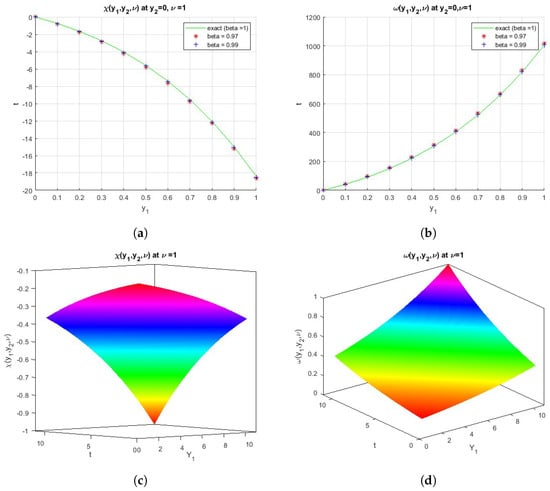
Figure 1. (a) The comparison between the exact and numerical solutions for $\chi (y_1,y_2,\nu )$. (b) The comparison between the exact and numerical solutions for $\omega (y_1,y_2,\nu )$. (c) The surface shows the function $\chi (y_1,y_2,\nu )$. (d) The surface shows the function $\omega (y_1,y_2,\nu )$.

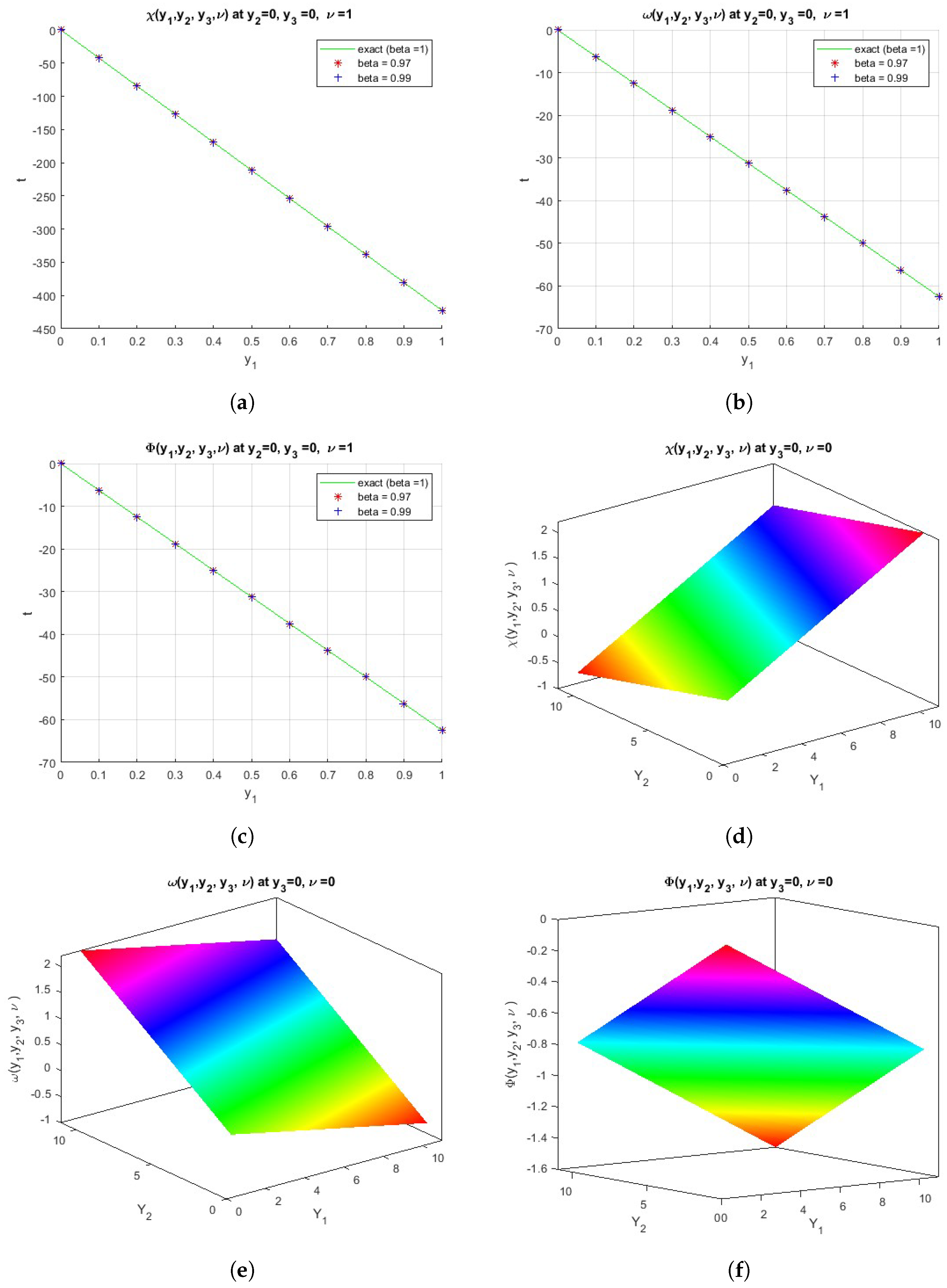
Figure 2. (a) The comparison between the exact and numerical solutions for $\chi (y_1,y_2,y_3,\nu )$. (b) The comparison between the exact and numerical solutions for $\omega (y_1,y_2,y_3,\nu )$. (c) The comparison between the exact and numerical solutions for $\Phi (y_1,y_2,y_3,\nu )$. (d) The surface shows the function $\chi (y_1,y_2,y_3,\nu )$. (e) The surface shows the function $\omega (y_1,y_2,y_3,\nu )$. (f) The surface shows the function $\Phi (y_1,y_2,y_3,\nu )$.

The comparison between the exact and numerical solutions for Equation (18) is shown in Figure 1a,b. We obtain the exact solution at $\beta =1$ and we use different values of $\beta$, such as ($\beta =0.97$, $\beta =0.99$), for the approximate solution. The surfaces in Figure 1c,d show the exact solutions of the functions $\chi (y_1,y_2,\nu )$ and $\omega (y_1,y_2,\nu )$ at $\nu =1$, respectively.

The comparison between the exact and numerical solutions for Equation (49) is shown in Figure 2a–c. We obtain the exact solution at $\beta =1$, and different values of $\beta$, such as ($\beta =0.97$, $\beta =0.99$), are used for the approximate solution. The surfaces in Figure 2d–f show the exact solutions of the functions $\chi (y_1,y_2,y_3\nu )$, $\omega (y_1,y_2,y_3,\nu )$ and $\Phi (y_1,y_2,y_3,\nu )$ at $y_3=0$ and $\nu =1$, respectively.

It is clear from the solutions of Equations (18) and (49) that the TGLTDM and FGLTDM have good agreement with the exact solutions to the problems.

6. Conclusions

In this article, we apply the TGLTDM and FGLTDM to solve the (2+1)- and (3+1)-dimensional Navier–Stokes systems of fractional partial differential equations, respectively. These methods have proven to be strong instruments that enable us to handle fractional-order differential equations and to reach the desired precision; it is only necessary to increase the number of iterations. Therefore, it can be found that the TGLTDM and FGLTDM are powerful methods in the search for exact as well as numerical solutions for fractional Navier–Stokes equations.

References

- Poincare, H. Memoires et observations. Sur l’equilibre d’une masse fluide animee d’un mouvement de rotation. Bull. Astron. Ser. I 1885, 2, 109–118. [Google Scholar]
- Wang, Y.; Zhao, Z.; Li, C.; Chen, Y.Q. Adomian’s method applied to Navier-Stokes equation with a fractional order. In Proceedings of the ASME 2009 IDETC/CIE, San Diego, CA, USA, 30 August–2 September 2009; pp. 1047–1054. [Google Scholar]
- Bazhlekova, E.; Jin, B.; Lazarov, R.; Zhou, Z. An analysis of the Rayleigh-Stokes problem for a generalized second-grade fluid. Numer. Math. 2015, 131, 1–31. [Google Scholar] [CrossRef] [PubMed]
- Zhou, Y.; Peng, L. Weak solutions of the time-fractional Navier-Stokes equations and optimal control. Comput. Math. Appl. 2017, 73, 1016–1027. [Google Scholar] [CrossRef]
- Kumar, S.; Kumar, D.; Abbasbandy, S.; Rashidi, M. Analytical solution of fractional Navier-Stokes equation by using modified Laplace decomposition method. Ain Shams Eng. J. 2014, 5, 569–574. [Google Scholar] [CrossRef]
- Mahmood, S.; Shah, R.; Khan, H.; Arif, M. Laplace Adomian Decomposition Method for Multi Dimensional Time Fractional Model of Navier-Stokes Equation. Symmetry 2019, 11, 149. [Google Scholar] [CrossRef]
- Mukhtar, S.; Shah, R.; Noor, S. The Numerical Investigation of a Fractional-Order Multi-Dimensional Model of Navier–Stokes Equation via Novel Techniques. Symmetry 2022, 14, 1102. [Google Scholar] [CrossRef]
- Singh, M.; Hussein, A.; Msmali; Tamsir, M.; Ahmadini, A.A.H. An analytical approach of multi-dimensional Navier-Stokes equation in the framework of natural transform. AIMS Math. 2024, 9, 8776–8802. [Google Scholar] [CrossRef]
- Albalawi, K.S.; Mishra, M.N.; Goswami, P. Analysis of the Multi-Dimensional Navier–Stokes equation by Caputo Fractional Operator. Fractal Fract. 2022, 6, 743. [Google Scholar] [CrossRef]
- Chu, Y.M.; Ali Shah, N.; Agarwal, P.; Dong Chung, J. Analysis of fractional multi-dimensional Navier–Stokes equation. Adv. Differ. Equ. 2021, 2021, 91. [Google Scholar] [CrossRef]
- Kim, H. The intrinsic structure and properties of Laplace-typed integral transforms. Math. Probl. Eng. 2017, 2017, 1762729. [Google Scholar] [CrossRef]
- Supaknaree, S.; Nonlapon, K.; Kim, H. Further properties of Laplace-type integral transform. Dyn. Syst. Appl. 2019, 28, 195–215. [Google Scholar] [CrossRef]
- Nuruddeen, R.I.; Akbar, Y.; Kim, H. On the application of G integral transform to nonlinear dynamical models with non-integer order derivatives. AIMS Math. 2022, 7, 17859–17878. [Google Scholar] [CrossRef]
- Eltayeb, H.; Mesloub, S. The New G-Double-Laplace Transforms and One-Dimensional Coupled Sine-Gordon Equations. Axioms 2024, 13, 385. [Google Scholar] [CrossRef]
- Eltayeb, H. Analytic Solution of the Time-Fractional Partial Differential Equation Using a Multi-G-Laplace Transform Method. Fractal Fract. 2024, 8, 435. [Google Scholar] [CrossRef]
- Bayrak, M.; Demir, A. A new approach for space-time fractional partial differential equations by residual power series method. Appl. Math. Comput. 2018, 336, 215–230. [Google Scholar]
Disclaimer/Publisher’s Note: The statements, opinions and data contained in all publications are solely those of the individual author(s) and contributor(s) and not of MDPI and/or the editor(s). MDPI and/or the editor(s) disclaim responsibility for any injury to people or property resulting from any ideas, methods, instructions or products referred to in the content. |
© 2024 by the authors. Licensee MDPI, Basel, Switzerland. This article is an open access article distributed under the terms and conditions of the Creative Commons Attribution (CC BY) license (https://creativecommons.org/licenses/by/4.0/).