On the Application of the Block Hybrid Methods to Solve Linear and Non-Linear First Order Differential Equations

Abstract

Block hybrid methods with intra-step points are considered in this study. These methods are implemented to solve linear and nonlinear single and systems of first order differential equations. The stability, convergence, and accuracy of the proposed methods are qualitatively investigated through the absolute and residual error analysis in some selected cases. A number of different numerical examples are tested to demonstrate the efficiency and applicability of the proposed methods. In this study we also implement the proposed methods to solve chaotic systems such as the Glukhvsky–Dolzhansky system, producing very comparable results to those already in the literature.

1. Introduction

Many equations that model physical or dynamical systems in science and engineering are initial value problems. As the name suggests, these are differential equations with prescribed initial conditions that specify the values of the unknown functions at the given specific points in the domain. These initial value problems (IVPs) specify how the systems evolve with time and variations of different parameters (if any), given the initial conditions. There are many initial value problems that we are interested in, that do not have any exact solutions or at least, analytical solutions, that we have figured out yet. In this paper, most of the examples used have exact solutions, since the main objective is the application of the proposed methods.

A plethora of studies have been conducted on block methods since the pioneering work of Shampine and Watts [1] on block implicit one-step methods. Block methods have been developed in order to obtain numerical solutions at more than one point at a time [1]. Brugnano and Trigianite [2] showed that the block methods contain the main and additional methods. Ramos et al. [3] developed a two-step continuous block method with intra-step points through interpolation and collocation. The study observed that the main advantages of the block methods are: (i) overcoming the overlapping pieces of solutions and (ii) that they are self-starting, thus avoiding the use of other methods to obtain starting solutions. Yap et al. [4] proposed the block hybrid collocation method with off-step points. Yap and Ismail [5] proposed the block-hybrid collocation method with three off-step points. Awari [6] studied a class of generalized two-step block hybrid numerical methods. Alharbi and Almatrafi [7] established exact and numerical solitary wave structures to the variant Boussinesq system. Xia [8] studied a generalized Riemann-type hydrodynamical equation and established the existence of a weak solution to the equation in a lower order Sobolev space. Alharbi and Almatrafi [9] presented exact solitary wave and numerical solutions for geophysical KdV equation.

Recently, Ononobgo et al. [10] developed a numerical algorithm for one and two-step hybrid block methods for a numerical solution of first order initial value problems using a method of collocation and Taylor’s series. This then gave a system of nonlinear equations, which was then solved to give a hybrid block method. More detailed work on hybrid block methods can be seen in Gear [11] and Motsa [12]. Yakubu et al. [13] derived the second derivation block hybrid method for the continuous integration of differential systems with the interval of integration.

Ramos and Rufai [14] proposed an implicit two-step block method that incorporates fourth derivatives for solving linear and nonlinear problems. Most recently, Motsa [15] presented a variation of the block methods for integrating systems of initial value problems.

In this study, we apply the newly developed block hybrid linear multi-step methods with off-step points to solve systems of linear and non-linear differential equations. It has been proved that the additional off-step points significantly improve the accuracy of these methods as well as ensuring consistency, zero-stability, and convergence [12]. This happens even if the grid-sizes are kept constant.

Block hybrid methods are used to find the approximate solutions of first order initial value problems of the form

$$\frac{dy}{dt}=f(t,y\left(t\right)),y\left(t_0\right)=y_0,$$

(1)

where $y_0$ is a given initial condition. The one-step method for solving initial value problems $\left(IVPs\right)$ and parabolic differential equations are considered in the implementations of the block hybrid algorithms. These $IVPs$ are solved over an interval $0\le t\le T$, which can be partitioned as $0=t_0<t_1<t_2<\cdots <t_{N-1}<t_N=T.$ The step size is calculated as $h=t_{n-1}-t_n,$ for $n=0,1,2,\cdots ,N-1.$ Now, the differential Equation (1) is solved in the N non-overlapping blocks, $[t_n,t_{n+1}],$ using the known initial condition $y\left(t_n\right)$ for $n=0,1,\cdots ,N-1.$ Then the $M-1$ points, called the off-steps or intra-step points, are introduced to improve the accuracy of the methods. We remark that M is the number of the collocation points.

The points used in the solution process in each block $t_n,t_{n+1}$ are $t_n,t_{n+p_1},t_{n+p_2},\cdots ,t_{tn+p_{M-1},t_{n+p_M}},$ where $t_{n+p_M}=t_{n+1},$ with $p_M=1.$ In the block hybrid method, equally spaced intra-step points defined by

$$t_{n+p_i}=t_n+\frac{i}{M}h=\left(n+\frac{i}{M}\right),$$

(2)

$i=1,2,\cdots ,m,$ are considered [12]. For each interval, say, $I_n$, the first order Equation (1) is solved to obtain a solution, $y^{n+1}\left(t\right).$ The solution in the first interval for example is denoted by $y^{\left(1\right)}\left(t_0\right)=y_0$ and on the subsequent intervals $I_n$ (for $n=1,2,\cdots ,N-1),$ as $y^{(n+1)}\left(t_n\right)=y\left(n\right)\left(t_n\right).$

Motsa [12] showed that the block hybrid method with the intra-step points $p_1,p_2,\cdots ,p_{M-1}$ has the form

$$y_{n+p_i}=y_n+h{\beta }_i{f}_n+h\sum _{j=1}^m{\alpha }_{i,j}{f}_{n+p_j},$$

(3)

$i=1,2,\cdots ,M$ where ${\alpha }_{i,j}$ and ${\beta }_i$ are known constants that depend on the nature of the intra-step points.

2. The Solution Method

Following Motsa [12], the block hybrid method for first order differential equations is based on approximating the exact solution $y\left(t\right)$ of the linear or non-linear differential Equation (1) by

$$y\left(t\right)\approx Y\left(t\right)=\sum _{k=0}^{M+1}{c}_{n,k}{(t-t_n)}^k,$$

(4)

where $c_{n,i}$ are the unknown coefficients in the $[t_n,t_{n+1}]$ block. With the coefficients $c_{n,i}$ being obtained from a system of $M+2$ equations with $M+2$ unknowns generated from

$$\begin{array}{ccc}\hfill & & {\dot{Y}}_{n+p_i}=f(t_{n+p_i},y_{n+p_i}),i=0,1,2,\cdots ,M\hfill \end{array}$$

(5)

$$\begin{array}{ccc}& & Y\left(t_n\right)=c_{n,0}=y_n,n=0,1,\cdots ,N-1,\hfill \end{array}$$

(6)

where the dot denotes differentiation with respect to time $t.$ As clearly explained in Motsa [12], the unknown constants $c_{n,k}$ are generated through Mathematica code. The code is as follows:

$$\begin{array}{ccc}\hfill M& =& 2;\hfill \\ \hfill points& =& Table\left[p_i=i/M,\{i,\theta ,M\}\right];\hfill \\ \hfill Table[t_{n+p_i}& =& (n+p_i)\times h,\{i,\theta ,M\}];\hfill \\ \hfill Y& =& Sum[c_{n,k}\times {(t-t_n)}^k,\{k,\theta ,M\}];\hfill \\ \hfill equations& =& Table[(D[Y,t]/t\to t_{n+p_i})\approx f_{n+p_i},\{i,\theta ,M\}]//simply;\hfill \\ \hfill unknowns& =& Table[c_{n,i},\{i,\theta ,M+1\}];\hfill \\ \hfill initial& =& c_{n,\theta }\approx \approx y_n;\hfill \\ \hfill Allequations& =& Join[equations,\{initial\left\}\right];\hfill \\ \hfill solutions& =& Solve[Allequations,unknowns]\hfill \end{array}$$

Upon solving the system of equations that arise from Equation (5), we can have $c_{n,0}=y_n,$ and $c_{n,1}=f_n$ for all values M. These $c_{n,k}$ coefficients for $k\ge 2$ are given for example, when $M=2,$

$$\begin{array}{ccc}& & c_{n,2}=-\frac{3f_n+f_{n+1}-4f_{n+\frac{1}{2}}}{2h},c_{n,3}=\frac{2\left(f_n+f_{n+1}-2f_{n+\frac{1}{2}}\right)}{3h^2}.\hfill \end{array}$$

(7)

Details of $M\ge 3$ can be found in the study by Motsa [12]. We then obtain the block hybrid method equation by substituting the expressions for $c_{n,k}$ in the approximation $Y\left(t\right)$ and by evaluating the result at the collocation points $t_{n+p_i}$ for $i=1,2,\cdots ,M.$ When the nodes are equally spaced, say, $\{0,\frac{1}{2},1\}$ with $M=2,$ we get

$$\begin{array}{ccc}& & y_{n+\frac{1}{2}}=y_n+\frac{1}{24}h\left(5f_n-f_{n+1}+8f_{n+\frac{1}{2}}\right),\hfill \\ & & y_{n+1}=y_n+\frac{1}{6}h\left(f_n+f_{n+1}+4f_{n+\frac{1}{2}}\right).\hfill \end{array}$$

(8)

The above equation can be written in matrix form as follows:

$$\begin{array}{c}\hfill \left[\begin{array}{c}{y}_{n+\frac{1}{2}}\\ y_{n+1}\end{array}\right]=\left[\begin{array}{c}{y}_n\\ y_n\end{array}\right]+h\left[\begin{array}{c}\frac{5f_n}{24}\\ \frac{f_n}{6}\end{array}\right]+h\left[\begin{array}{cc}\frac{1}{3}& -\frac{1}{24}\\ \frac{2}{3}& \frac{1}{6}\end{array}\right]\left[\begin{array}{c}{f}_{n+\frac{1}{2}}\\ f_{n+1}\end{array}\right].\end{array}$$

(9)

The block hybrid method with the intra-step points $p_1,p_2,p_3,\cdots ,p_{m-1}$, which in general is given by (3).

Equation (3), can be written in matrix as

$$Y_{n+m}=Y_n+h{A}_m{F}_{n+m}+h{B}_m{F}_n,$$

(10)

where the respective coefficient matrices are defined as

$$\begin{array}{c}\hfill A_m=\left[\begin{array}{cccc}{\alpha }_{1,1}& {\alpha }_{1,2},& \cdots ,& {\alpha }_{1,m}\\ {\alpha }_{2,1}& {\alpha }_{2,2}& \cdots & {\alpha }_{2,m}\\ ⋮& ⋮& \ddots & ⋮\\ {\alpha }_{m,1}& {\alpha }_{m,2}& \cdots & {\alpha }_{m,m}\end{array}\right],B_m=\left[\begin{array}{cccc}{\beta }_1& 0& \cdots & 0\\ 0& {\beta }_2& \cdots & 0\\ ⋮& ⋮& \ddots & ⋮\\ 0& 0& \cdots & {\beta }_m\end{array}\right],\end{array}$$

(11)

and the column vectors are:

$$\begin{array}{ccc}& & Y_{n+m}={\left[y_{n+p_1},y_{n+p_2},\cdots ,y_{n+p_m}\right]}^T,F_{n+m}={\left[f_{n+p_1},f_{n+p_2},\cdots ,f_{n+p_m}\right]}^T,\hfill \end{array}$$

(12)

$$\begin{array}{ccc}& & Y_n={\left[y_n,y_n,\cdots ,y_n\right]}^T,F_n={\left[f_n,f_n,\cdots ,f_n\right]}^T.\hfill \end{array}$$

(13)

The coefficient matrices $A_m$ and $B_m,$ when $M=1,2,3,4,5$ are

$$A_1=\frac{1}{2},B_1=\frac{1}{2},$$

$$A_2=\left[\begin{array}{cc}\frac{1}{3}& -\frac{1}{24}\\ \frac{2}{3}& \frac{1}{6}\end{array}\right],B_2=\left[\begin{array}{cc}\frac{1}{24}& \frac{1}{6}\\ -\frac{1}{6}& \frac{1}{3}\end{array}\right],$$

$$A_3=\left[\begin{array}{ccc}\frac{19}{72}& -\frac{5}{72}& \frac{1}{72}\\ \frac{4}{9}& \frac{1}{9}& 0\\ \frac{3}{8}& \frac{3}{8}& \frac{1}{8}\end{array}\right],B_3=\left[\begin{array}{ccc}-\frac{1}{72}& \frac{13}{216}& \frac{17}{216}\\ -\frac{4}{27}& \frac{1}{9}& \frac{4}{27}\\ -\frac{7}{24}& \frac{5}{24}& \frac{5}{24}\end{array}\right],$$

$$A_4=\left[\begin{array}{cccc}\frac{323}{1440}& -\frac{11}{120}& \frac{53}{1440}& -\frac{19}{2880}\\ \frac{31}{90}& \frac{1}{15}& \frac{1}{90}& -\frac{1}{360}\\ \frac{51}{160}& \frac{9}{40}& \frac{21}{160}& -\frac{3}{320}\\ \frac{16}{40}& \frac{2}{15}& \frac{16}{45}& \frac{7}{90}\end{array}\right],B_4=\left[\begin{array}{cccc}-\frac{71}{2880}& \frac{17}{640}& \frac{19}{480}& \frac{263}{5760}\\ -\frac{11}{90}& \frac{2}{45}& \frac{13}{180}& \frac{31}{360}\\ -\frac{9}{40}& \frac{51}{640}& \frac{33}{320}& \frac{81}{640}\\ -\frac{59}{180}& \frac{7}{60}& \frac{7}{60}& \frac{31}{180}\end{array}\right],$$

$$A_5=\left[\begin{array}{ccccc}\frac{1427}{7200}& -\frac{133}{1200}& \frac{241}{3600}& -\frac{173}{7200}& \frac{3}{800}\\ \frac{43}{150}& \frac{7}{225}& \frac{7}{225}& -\frac{1}{75}& \frac{1}{450}\\ \frac{219}{800}& \frac{57}{400}& \frac{57}{400}& -\frac{21}{800}& \frac{3}{800}\\ \frac{64}{225}& \frac{8}{75}& \frac{64}{225}& \frac{14}{225}& 0\\ \frac{25}{96}& \frac{25}{144}& \frac{25}{144}& \frac{25}{96}& \frac{19}{288}\end{array}\right],B_5=\left[\begin{array}{ccccc}-\frac{187}{7200}& \frac{113}{9000}& \frac{809}{\mathrm{36,000}}& \frac{61}{2250}& \frac{1073}{\mathrm{36,000}}\\ -\frac{229}{2250}& \frac{4}{2250}& \frac{89}{2250}& \frac{113}{2250}& \frac{127}{2250}\\ -\frac{723}{4000}& \frac{63}{2000}& \frac{9}{160}& \frac{147}{2000}& \frac{333}{4000}\\ -\frac{292}{1125}& \frac{52}{1125}& \frac{76}{1125}& \frac{22}{225}& \frac{124}{1125}\\ -\frac{487}{1440}& \frac{11}{180}& \frac{113}{1440}& \frac{47}{360}& \frac{193}{1440}\end{array}\right].$$

To validate the block hybrid method results obtained in this study, we consider the equation:

$$y^{\prime }=y-t^2+1,0\le t\le 2,y\left(0\right)=0.5,$$

(14)

with the exact solution

$$y\left(t\right)={(t+1)}^2-0.5e^t.$$

(15)

Table 1 clearly shows the high accuracy of the block hybrid method even with very high step sizes. The results from the fourth order Ruge–Kutta method were generated with the step size $h=0.02$, whilst those of the BHM were generated with the step size $h=0.2.$

Table 1. Maximum Errors for HBM (with $h=0.2$) and RK4 (with $h=0.02$).

t	Exact Solution	BHM-Errors	RK4-Errors
0	0.5	0	0
0.2	0.829298620919917	$2\times {10}^{-15}$	$5.7\times {10}^{-10}$
0.4	1.214087651179369	$4\times {10}^{-15}$	$1.2\times {10}^{-9}$
0.6	1.648940599804753	$7\times {10}^{-15}$	$2.0\times {10}^{-9}$
0.8	2.127229535753778	$1.2\times {10}^{-14}$	$2.9\times {10}^{-9}$
1.0	2.640859085770495	$1.8\times {10}^{-14}$	$3.9\times {10}^{-9}$
1.2	3.179941538631752	$2.5\times {10}^{-14}$	$5\times {10}^{-9}$
1.4	3.732400016577701	$5.2\times {10}^{-14}$	$6.3\times {10}^{-9}$
1.6	4.283483787802496	$5.2\times {10}^{-14}$	$7.8\times {10}^{-9}$
1.8	4.815176267793600	$7.5\times {10}^{-14}$	$9.5\times {10}^{-9}$
2.0	5.305471950534773	$9.9\times {10}^{-14}$	$1.1\times {10}^{-8}$

We note that the block hybrid method gives a consistently superior result, which can be clearly observed in Table 2.

Table 2. Comparisons of errors of the results generated by the BHM and those obtained by Burden and Faires [16].

${\mathit{t}}_0$	Exact	BHM	Error	Adams $4\mathbf{th}$ Order Predictor-Corrector Method	Error (Burden and Faires [16])
0.0	0.5000000	0.5000000	0	0.5000000	0
0.2	0.8292986	0.8292986	0	0.8292933	0.0000053
0.4	1.2140877	1.2140877	0	1.21407762	0.0000114
0.6	1.6489406	1.6489406	0	1.6489220	0.0000186
0.8	2.1272295	2.1272295	0	2.1272056	0.0000239
1.0	2.6408591	2.6408591	0	2.6408286	0.0000305
1.2	3.1799415	3.1799415	0	3.1799026	0.0000389
1.4	3.7324000	3.7324000	0	3.7323505	0.0000495
1.6	4.2834838	4.2834838	0	4.2834208	0.0000630
1.8	4.8151763	4.8151763	0	4.8150964	0.0000799
2.0	5.3054720	5.3054720	0	5.3053707	0.0001013

Local Truncation Error

Given a function $y\left(t\right)$, which is sufficiently differentiable, we can express the block hybrid methods following Motsa [17], in terms of the linear ${\ell }_i,$ with

$${\ell }_i[y\left(t_n\right);h]=y(t_n+h{p}_i)-y\left(t_n\right)-h{\beta }_i{y}^{\prime }\left(t_n\right)-h\sum _{j=1}^M{\alpha }_{i,j}{y}^{\prime }(t_n+h{p}_j),i=1,2,\cdots ,M.$$

(16)

We can then expand the terms of $y(t_n+h{p}_i)$ and $y^{\prime }(t_n+h{p}_i)$ using Taylor series about $t_n$ to obtain

$${\displaystyle {\ell }_i[y\left(t_n\right);h]=C_{i,0}y\left(t_n\right)+C_{i,1}h{y}^{\prime }\left(t_n\right)+C_{i,2}{h}^2{y}^{″}\left(t_n\right)+\cdots +C_{i,q}{h}^q{y}^{\left(q\right)}\left(t_n\right),}$$

(17)

where $C_{i,0},C_{i,1},\cdots C_{i,q}$ are constants. The method is said to be an order of q if

$$\widehat{C_0}=\widehat{C_1}=\cdots =\widehat{C_{q+1}}=0\mathrm{and}\widehat{C_{q+2}}\ne 0.$$

Upon expanding Equation (16) using Taylor series we get:

$${\displaystyle {\ell }_i[y\left(t_n\right);h]=\sum _{k=1}^m\frac{p_i^k}{k!}{h}^k{y}^{\left(k\right)}\left(t_n\right)-h{\beta }_i{y}^{\prime }\left(t_n\right)-\sum _{k=1}^m\frac{p_i^k}{k!}\sum _{j=1}^M{\alpha }_{i,j}{p}_j^{k-1}{y}^{\left(k\right)}\left(t_n\right)+O\left(h^{m+1}\right),}$$

(18)

where m is a positive integer. The above Equation (18) can be expanded to obtain:

$$\begin{array}{ccc}\hfill & & {\displaystyle {\ell }_i[y\left(t_n\right);h]=\sum _{k=1}^{M+1}\frac{p_i^k}{k!}{h}^k{y}^{\left(k\right)}\left(t_n\right)-h{\beta }_i{y}^{\prime }\left(t_n\right)-\sum _{k=1}^{M+1}\frac{p_i^k}{k!}\sum _{j=1}^M{\alpha }_{i,j}{p}_j^{k-1}{y}^{\left(k\right)}\left(t_n\right)}\hfill \\ & & +\frac{h^{M+2}}{(M+2)!}\left[p_i^{M+2}-(M+2)\sum _{j=1}^M{\alpha }_{i,j}{p}_j^{M+1}\right]y^{(M+2)}\left(t_n\right)+O\left(h^{M+3}\right)\hfill \end{array}$$

(19)

Motsa [17] showed that from numerical evaluation the sum of the first three terms of Equation (19) is zero. Therefore the truncation error for the block hybrid with $M+1$ nodes in the interval $[t_n,t_{n+1}]$ is

$${\ell }_i[y\left(t_n\right);h]=\frac{h^{M+2}}{(M+2)!}\left[p_i^{M+2}-(M+2)\sum _{j=1}^M{\alpha }_{i,j}{p}_j^{M+1}\right]y^{(M+2)}\left(t_n\right)+O\left(h^{M+3}\right).$$

(20)

Thus, the order of the block hybrid method for say $3nodes$ will be 5, which is the least order of applying this method. We also remark that as M increases so does the order of convergence. This then increases the accuracy of the method, as will be observed later in this study.

3. Applications

Randomly selected numerical experiments are studied to show the performance and viability of the proposed methods.

3.1. Numerical Linear Examples

We consider a general linear first order equation of the form:

$$\dot{y}=f(t,y)=\psi \left(t\right)+\varphi \left(t\right)y,t_0<t<t_T,$$

(21)

where $\psi$ and $\varphi$ are known functions of $t.$ Following Motsa [12], the block hybrid scheme for solving linear equations is given by

$$y_{n+p_i}=y_n+h{\beta }_i\left({\psi }_n+{\varphi }_n{y}_n\right)+h\sum _{j=1}^n{\alpha }_{i,j}\left({\psi }_{n+p_j}+{\varphi }_{n+p_j}{y}_{n+p_j}\right),i=1,2,3,\cdots ,M.$$

(22)

The above Equation (22) can be expressed in matrix form as:

$$A_n{Y}_n=B_n,$$

(23)

with

$$\begin{array}{c}\hfill A_n=\left[\begin{array}{cccc}1& 0& \cdots & 0\\ 0& 1& \cdots & 0\\ ⋮& ⋮& \ddots & \ddots \\ 0& 0& \cdots & 1\end{array}\right]-h{A}_m\left[\begin{array}{cccc}{\varphi }_{n+p_1}& 0& \cdots & 0\\ 0& {\varphi }_{n+p_2}& \cdots & 0\\ ⋮& \cdots & \ddots & ⋮\\ 0& 0& \cdots & {\varphi }_{n+p_m}\end{array}\right].\end{array}$$

(24)

$$\begin{array}{c}\hfill B_n=\left[\begin{array}{c}{y}_n\\ y_n\\ ⋮\\ y_n\end{array}\right]+h{A}_m\left[\begin{array}{c}{\psi }_{n+p_1}\\ {\psi }_{n+p_2}\\ ⋮\\ {\psi }_{n+p_m}\end{array}\right]+h{B}_m\left[\begin{array}{cccc}{\psi }_n+{\varphi }_n{y}_n& {\psi }_n+\varphi y_n& ⋮& {\psi }_n+{\varphi }_n{y}_n\end{array}\right],\end{array}$$

(25)

and

$$Y_n={\left[y_{n+p_1},y_{n+p_2},\cdots ,y_{n+p_M}\right]}^T.$$

(26)

3.1.1. Linear Example 1

In this section we are going to randomly selected examples to demonstrate the efficiency of the block-hybrid method. First, we consider the following example;

$$y^{\prime }=t{e}^{3t}-2y,0\le t\le 1,y\left(0\right)=0,$$

(27)

with an exact solution given as

$$y\left(t\right)=\frac{1}{5}t{e}^{3t}-\frac{1}{25}{e}^{3t}+\frac{1}{25}{e}^{-2t}.$$

(28)

In this case, we have $\psi \left(t\right)=t{e}^{3t}$ and $\varphi \left(t\right)=-2.$ As can be clearly observed in Figure 1, the accuracy of the method greatly increases as M increases. Figure 2 shows that there is an excellent agreement between the exact and the approximate solutions. This can be seen also on the errors of order ${10}^{-15}$ in Figure 1.

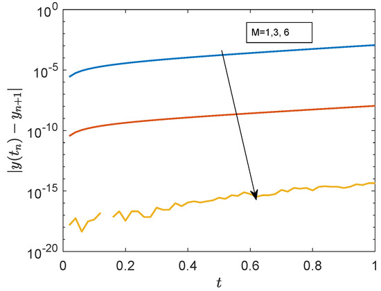
Figure 1. Errors for example 1.

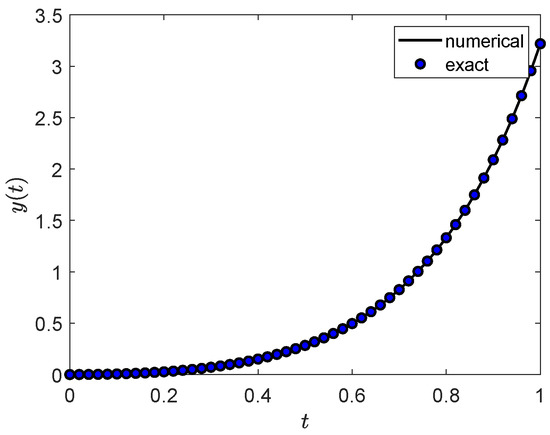
Figure 2. Graphs of the exact and approximate solutions for example 1.

3.1.2. Linear Example 2

The example below was randomly selected to demonstrate the robustness of the proposed method.

$$y^{\prime }=\frac{2-2ty}{t^2+1},0\le t\le 1,y\left(0\right)=0,$$

(29)

with exact solution given as

$$y\left(t\right)=\frac{2t+1}{t^2+1}.$$

(30)

In example 2, $\psi \left(t\right)=\frac{2}{t^2+1}$ and $\varphi \left(t\right)=-\frac{2t}{t^2+1}.$ In Figure 3, we observe that the accuracy is up to the ${10}^{-13}$ error levels, which is highly commendable. This is observed further in Figure 4, which shows an excellent agreement between the exact and approximate solutions.

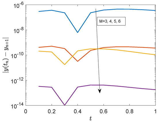
Figure 3. Errors for example 2.

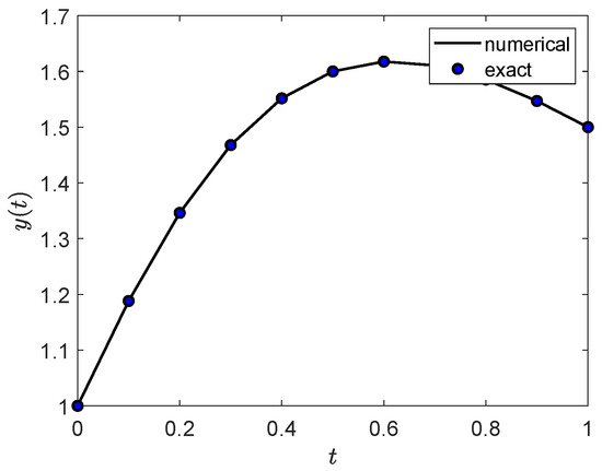
Figure 4. Graphs of the exact and approximate solutions for example 2.

3.1.3. Linear Example 3

The example below was chosen to illustrate the efficiency of the BHM.

$$y^{\prime }=\frac{-4ty}{t^2+1}+\frac{2}{{(1+t)}^2},0\le t\le 6,y\left(0\right)=1,$$

(31)

with exact solution given as

$$y\left(t\right)=\frac{2t+1}{{(t^2+1)}^2}.$$

(32)

In this example, $\psi \left(t\right)=\frac{2}{{(1+t)}^2}$ and $\varphi \left(t\right)=-\frac{4t}{1+t^2}.$ The exact and approximate solutions are depicted in Figure 5. We observe that there is an excellent agreement between the two sets of solutions. This can also be perceived in Figure 6 which depicts a very high level of accuracy.

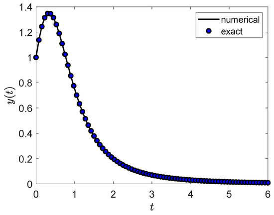
Figure 5. Graphs of the exact and approximate solutions for example 3.

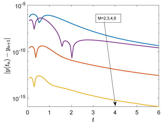
Figure 6. Errors for example 3.

3.1.4. Linear Example 4

This example was randomly selected to illustrate the robustness of the proposed method.

$$y^{\prime }=-2y+t^3{e}^{-2t}0\le t\le 1,y\left(0\right)=1,$$

(33)

with exact solution given as

$$y\left(t\right)=\frac{e^{-2t}}{4}(t^4+4).$$

(34)

In this example, $\psi \left(t\right)=t^3{e}^{-2t}$ and $\varphi \left(t\right)=-$2. Figure 7 and Figure 8 depict, respectively, the errors and the comparisons of the exact and approximate solutions. Moreover, we observe the robustness of the numerical method in solving these types of first order initial value problems.

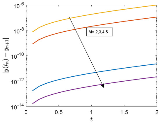
Figure 7. Errors for example 4.

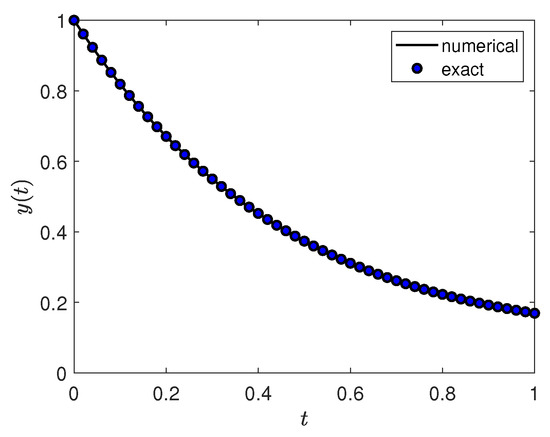
Figure 8. Graphs of the exact and approximate solutions for example 4.

3.2. Numerical Nonlinear First Order Differential Equations

In this subsection, we examine some few selected non-linear first order differential equations to demonstrate the strength of the methods under discussion. The quasi-linearization method is used to linearize the equations first. The non-linear first order differential equations are first linearized to enable us to apply the BHMs. We consider a non-linear first order differential equation of the form

$$y^{\prime }=\ell \left(t\right)y+\aleph (t,y),$$

(35)

where, $\ell \left(t\right)$ is a known function of t, and $\aleph (t,y)$ is a nonlinear function of $y.$ In this study, we will use the quasi-linearization (QLM) iteration method, developed by Bellman and Kalaba [18]. The QLM approach is based on Taylor series expansion of the nonlinear term $\aleph (t,y).$ In this method, we assume that the difference between the current and previous iteration $(y_{r+1}-y_r)$ is small. We have, $\aleph (t,y)\approx \aleph (t,y_r)+\frac{\partial \aleph }{\partial y}(y_{r+1}-y_r).$ This gives the linearized approximation Equation (35)

$$y_{r+1}^{\prime }=\ell \left(t\right)y_{r+1}+\aleph (t,y_r)+\frac{\partial \aleph }{\partial y}\aleph y_{r+1}-y_r.$$

(36)

We then apply the block hybrid method scheme with

$$\begin{array}{c}\hfill \varphi \left(t\right)=\ell \left(t\right)+\frac{\partial \aleph }{\partial y},\psi \left(t\right)=\aleph (t,y_r)-y_r\frac{\partial \aleph }{\partial y}.\end{array}$$

(37)

We discuss some few randomly selected examples to demonstrate the strength of the block-hybrid method.

3.2.1. Nonlinear Example 1 (Riccati Equation)

This example was conveniently selected to demonstrate the robustness of the proposed method. The riccati equation though nonlinear its exact solution can easily be found.

$$y^{\prime }=1+\frac{y}{t}+\frac{y^2}{t^2},1\le t\le 3,y\left(1\right)=0,$$

(38)

with the exact solution given as

$$y\left(t\right)=ttan(lnt).$$

(39)

Following Equation (36), we deduce that, $\ell \left(t\right)=\frac{1}{t}$ and $\aleph (t,y)=1+\frac{y^2}{t^2}$ with $\frac{\partial \aleph }{\partial y}=\frac{2y}{t^2}.$ Therefore,

$${\displaystyle {\dot{y}}_{r+1}=\left(\frac{1}{t}+\frac{2y_r}{t^2}\right)y_{r+1}+1-\frac{y_r^2}{t^2},}$$

(40)

with $\varphi \left(t\right)=\frac{1}{t}+\frac{2y_r}{t^2},$$\psi \left(t\right)=1-\frac{y_r^2}{t^2}.$ We then apply the block-hybrid method to solve the resultant linear equations and the results as depicted in Figure 9 and Figure 10. Again, we see that the current method gives an accuracy as high as ${10}^{-14}$, which is highly commendable.

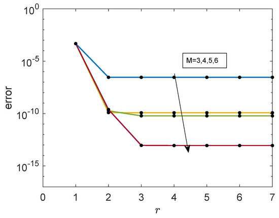
Figure 9. Errors for nonlinear example 1 as M is increasing.

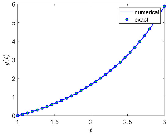
Figure 10. Graphs of the exact and approximate solutions for example 1.

3.2.2. Nonlinear Example 2

This example was randomly selected to demonstrate the robustness of the proposed BHM.

$$y^{\prime }=\frac{y}{3}+\frac{t{y}^4}{6},0\le t\le 1,y\left(0\right)=-2,$$

(41)

with the exact solution given as

$$y\left(t\right)=-\frac{2}{{(4t-4+5e^{-t})}^{\frac{1}{3}}}.$$

(42)

We have $\ell \left(t\right)=\frac{1}{3}$ and $\aleph (t,y_r)=\frac{t{y}^4}{6},$ with $\frac{\partial \aleph }{\partial y_r}=\frac{2t{y}_r^3}{3}.$

Hence,

$${\dot{y}}_{r+1}=\left(\frac{1}{3}+\frac{2t{y}_r^3}{3}\right)y_{r+1}-\frac{t{y}_r^4}{2}.$$

(43)

We have, $\varphi \left(t\right)=\frac{1}{3}+\frac{2t{y}_r^3}{3}$ and $\psi \left(t\right)=-\frac{t{y}_r^4}{2}.$ Upon application of the BHMs on Equation (43) we obtain the results, which are depicted in Figure 11 and Figure 12.

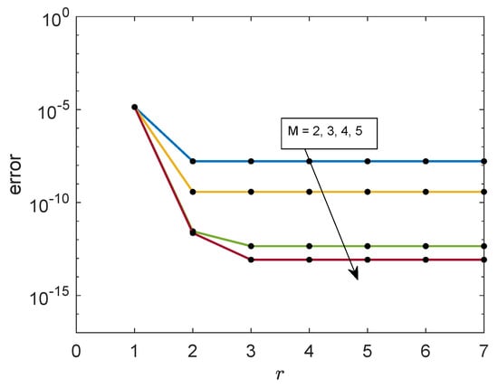
Figure 11. Errors for non-linear example 2.

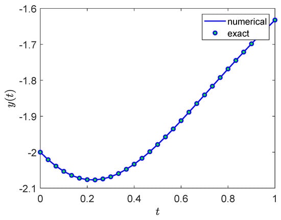
Figure 12. Graphs of the exact and approximate solutions for example 2.

3.3. Nonlinear Systems of First Order Equations

Lastly, we apply the block-hybrid methods to non-linear systems of N equations of the form:

$$\begin{array}{ccc}& & {\dot{y}}_1=f_1(t,y_1,y_2,\cdots ,y_N)={\ell }_1(t,y_2,y_3,\cdots ,y_N)y_1+{\aleph }_1(t,y_1,y_2,\cdots ,y_N),\hfill \\ & & {\dot{y}}_2=f_2(t,y_1,y_2,\cdots ,y_N)={\ell }_2(t,y_1,y_3,\cdots ,y_N)y_2+{\aleph }_2(t,y_1,y_2,\cdots ,y_N),\hfill \\ & & ⋮\hfill \\ & & \dot{y_k}=f_k(t,y_1,y_2,\cdots ,y_N)={\ell }_k(t,y_1,y_3,y_{k-1},y_{k+1},\cdots ,y_N)y_k+{\aleph }_2(t,y_1,y_2,\cdots ,y_N),\hfill \\ & & ⋮\hfill \\ & & \dot{y_N}=f_N(t,y_1,y_2,\cdots ,y_N)={\ell }_N(t,y_1,y_3,\cdots ,y_{N-1})y_N+{\aleph }_N(t,y_1,y_2,\cdots ,y_N),\hfill \end{array}$$

(44)

where ${\ell }_k$ is the component of the non-linear function that is a coefficient to $y_k$ in the $k-\mathrm{th}$ equation and ${\aleph }_k\left(t\right)$ is the remaining component which may or may not be a non-linear function for $k=1,2,\cdots ,N.$ At each iteration, denoted by $r+1,$ the decoupling iterative scheme takes the form:

$$\begin{array}{ccc}\hfill & & {\dot{y}}_{k,r+1}={\ell }_k(t,y_{1,r+1},y_{2,r+1},\cdots ,y_{k-1,r+1},y_{k+1,r},y_{N,r})y_{k,r+1}\hfill \\ & & +{\aleph }_k(t,y_{1,r+1},y_{2,r+1},\cdots ,y_{k-1,r+1},y_{k+1,r},y_{N,r}),\hfill \end{array}$$

(45)

for each $k=1,2,\cdots ,N.$ The block-hybrid method for a linear first order Equation (37) can now be applied to the above Equation (45) with ${\varphi }_k={\ell }_k(t,y_{1,r+1},y_{2,r+1},\cdots ,y_{k-1,r+1},y_{k+1,r},y_{N,r})$ and ${\psi }_k={\aleph }_k(t,y_{1,r+1},y_{2,r+1},\cdots ,y_{k-1,r+1},y_{k+1,r},y_{N,r}),$ for each $k=1,2,\cdots ,N.$ The scheme is now called the Relaxation Block Hybrid Method (Motsa [12]), for solving these systems of equations. We then develop a quasilinearization scheme by applying the linearization sequentially in $y_k$ only to obtain

$$\begin{array}{ccc}\hfill & & {\dot{y}}_{k,r+1}={\ell }_k(t,y_{1,r+1},y_{2,r+1},\cdots ,y_{k-1,r+1},y_{k+1,r},y_{N,r})y_{k,r+1}\hfill \\ & & +{\aleph }_k(t,y_{1,r+1},y_{2,r+1},\cdots ,y_{k-1,r+1},y_{k+1,r},y_{N,r})+\frac{\partial {\aleph }_k}{\partial y_k}(y_{r+1}-y_{k,r})\hfill \end{array}$$

(46)

The BHMs are then applied with ${\varphi }_k={\ell }_k+\frac{\partial {\aleph }_k}{\partial y_k},{\psi }_k={\aleph }_k-y_{k,r}\frac{\partial {\aleph }_k}{\partial y_k}.$ The BHM implemented with the quasilinearization (46) can be referred to as the Local Quazilinearization Block Hybrid Method (LQBHM) [12].

3.3.1. Nonlinear Systems, Example 1

We consider the following Lorenz system given by

$$\begin{array}{ccc}\hfill \dot{y_1}& =& \sigma (y_2-y_1),\hfill \\ \hfill \dot{y_2}& =& -y_1{y}_3+\rho y_1-y_2,\hfill \\ \hfill \dot{y_3}& =& y_1{y}_2-c{y}_3,\hfill \end{array}$$

(47)

with initial conditions $y_1\left(0\right)=1,y_2\left(0\right)=5,y_3\left(0\right)=10.$ The BHM parameters:

$$\begin{array}{c}\hfill {\varphi }_1=-\sigma ,{\psi }_1=\sigma y_2,{\varphi }_2=-1,{\psi }_2=-y_1{y}_3+\rho y_1,{\varphi }_3=-c,{\psi }_3=y_1{y}_2.\end{array}$$

We select some few graphical examples to demonstrate how powerful the proposed method is. We can clearly observe in Figure 13, Figure 14 and Figure 15 that the accuracy of the method increases as the number of iterations increases. An accuracy up to ${10}^{-14}$ is achieved by this method. In Figure 16, we observe the chaotic nature of the solutions. We observe that solutions exhibit irregular oscillations that persist as $t\to \infty$, but never repeat exactly. The motions are further aperiodic.

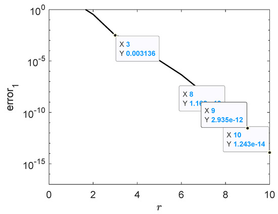
Figure 13. Errors for the Lorenz system.

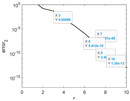
Figure 14. Errors for the Lorenz system.

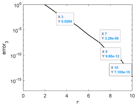
Figure 15. Errors for the Lorenz system.

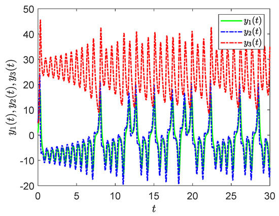
Figure 16. Plots of the solutions of $y_1,y_2,y_3$.

Figure 17, Figure 18, Figure 19, Figure 20, Figure 21 and Figure 22 depict phase portraits of the system when varying the system parameters. In this study we are not going to go into the physics and explanations of the portraits. Our focus is to generate accurate solutions, since the Lorenz equations have been the subject of hundreds of research papers, see for example Fang and Hao [19], and Hao et al. [20].

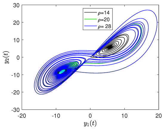
Figure 17. Phase portraits of $y_1$ and $y_2$ when varying $\rho$.

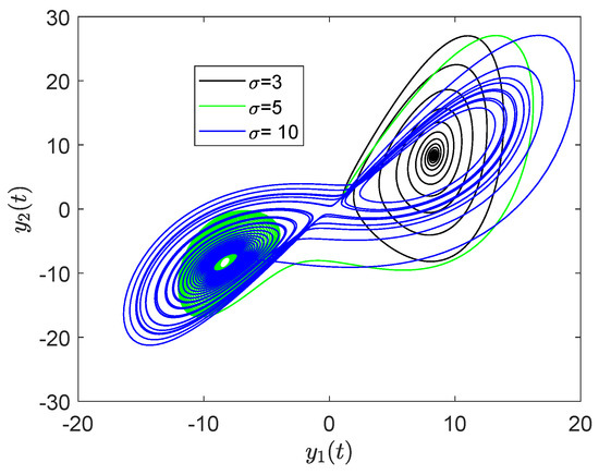
Figure 18. Phase portraits of $y_1$ and $y_2$ when varying $\sigma$.

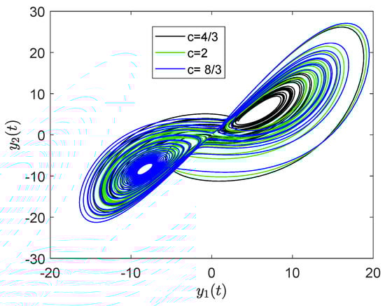
Figure 19. Phase portraits of $y_1$ and $y_2$ when varying c.

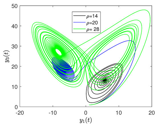
Figure 20. Phase portraits of $y_1$ and $y_3$ when varying $\rho$.

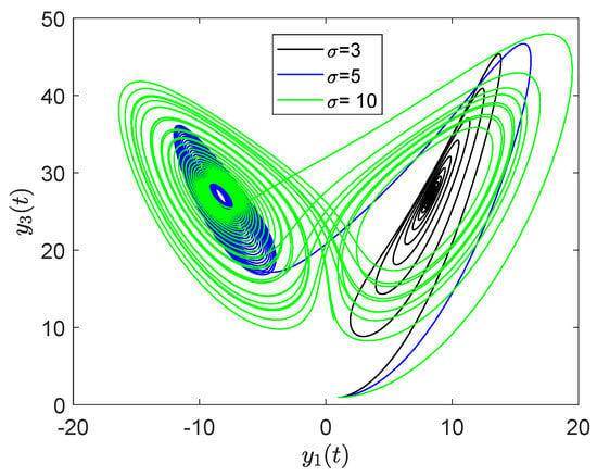
Figure 21. Phase portraits of $y_1$ and $y_3$ when varying $\sigma$.

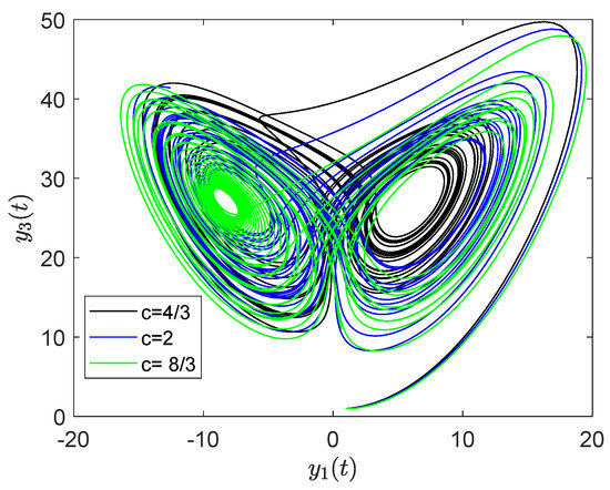
Figure 22. Phase portraits of $y_1$ and $y_3$ when varying c.

In Figure 23, Figure 24 and Figure 25, we display the $3D$ evolutions of the three trajectories when varying the three parameters. Fundamentally, the trajectories seem to exhibit similar shapes when varying the three parameters.

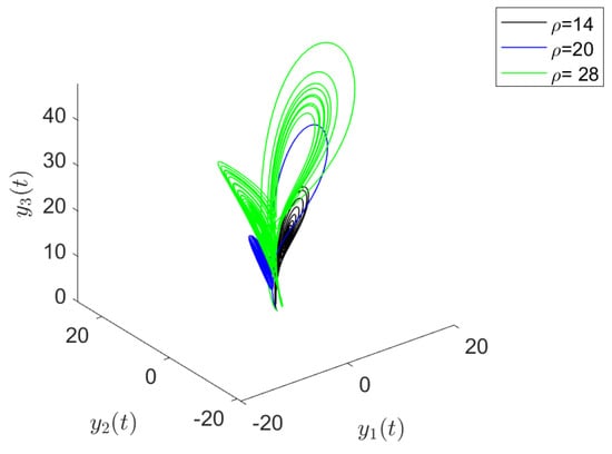
Figure 23. Phase portraits of $y_1$, $y_2$ and $y_3$ when varying $\rho$.

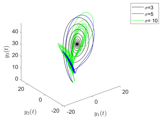
Figure 24. Phase portraits of $y_1$, $y_2$ and $y_3$ when varying $\sigma$.

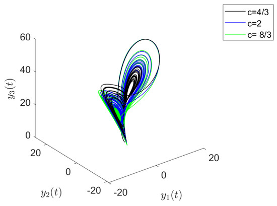
Figure 25. Phase portraits of $y_1$, $y_2$ and $y_3$ when varying c.

In Figure 26, Figure 27 and Figure 28, we display the phase portraits of $y_2$ and $y_3$ when varying the three parameters.

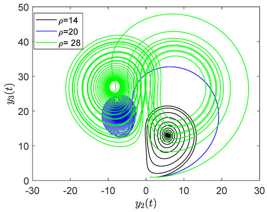
Figure 26. Phase portraits of $y_2$ and $y_3$ when varying $\rho$.

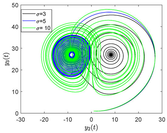
Figure 27. Phase portraits of $y_2$ and $y_3$ when varying $\sigma$.

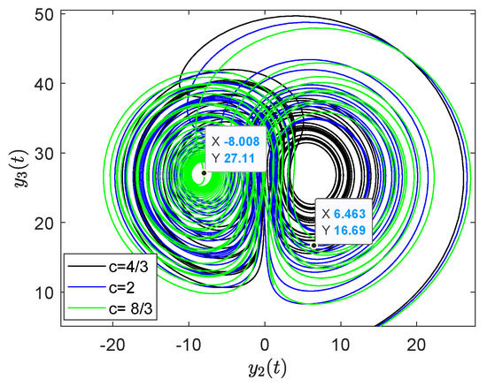
Figure 28. Phase portraits of $y_2$ and $y_3$ when varying c.

3.3.2. Nonlinear Systems, Example 2

Further, we consider the Glukhovsky–Dolzhanksy system (see Garashchuk et al. [21]) given by

$$\begin{array}{ccc}\hfill \dot{y_1}& =& -\sigma (y_1-y_2)-a{y}_2{y}_3,\hfill \\ \hfill \dot{y_2}& =& r{y}_1-y_2-y_1{y}_3,\hfill \\ \hfill \dot{y_3}& =& -b{y}_3+y_1{y}_2,\hfill \end{array}$$

(48)

where $\sigma ,r,b$ are the physical parameters. This system has an additional nonlinear term compared to the Lorenz system. This extra nonlinear term leads to essential differences in the analytical structure and dynamics of the system. This system describes the following physical processes: convective fluid motion in a ellipsoidal rotating cavity, a rigid body rotation in a resisting medium, the forced motion of a gyrostat, and a convective motion in harmonically oscillating horizontal fluid. Selected phase portraits are depicted in Figure 29, Figure 30, Figure 31 and Figure 32. Figure 29 shows that very chaotic patterns are initially exhibited and thereafter the flows exhibit somehow steady states as $t\to \infty$.

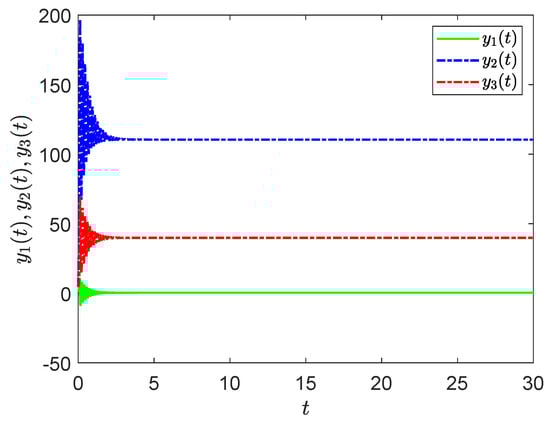
Figure 29. Solution profiles of the Glukhovsky–Dolzhanksy system of equations.

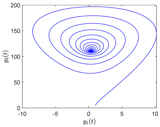
Figure 30. Phase portraits of $y_1$ and $y_2$.

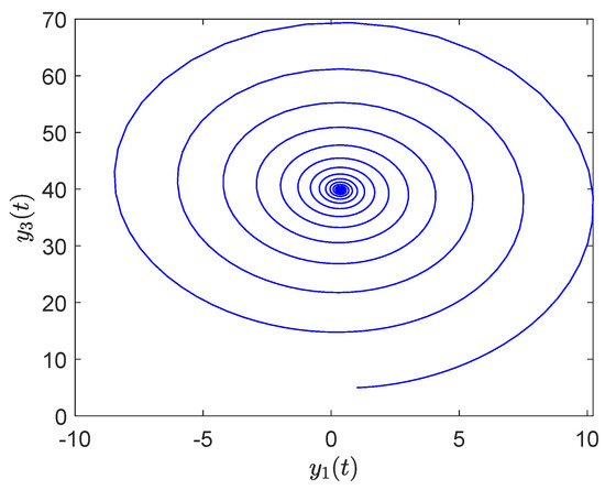
Figure 31. Phase portraits of $y_1$ and $y_3$.

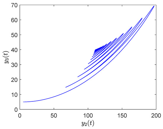
Figure 32. Phase portraits of $y_2$ and $y_3$.

3.3.3. Nonlinear Systems Example 3

Consequently, the study considers a dissipative chaotic system with no equilibrium given by

$$\begin{array}{ccc}\hfill \dot{y_1}& =& y_2,\hfill \\ \hfill \dot{y_2}& =& y_1+y_2{y}_3,\hfill \\ \hfill \dot{y_3}& =& y_1^2-4y_2^2+1,\hfill \end{array}$$

(49)

This dissipative structure/system is characterized by the spontaneous appearance of symmetry breaking (anisotropy) and the formation of complex and chaotic structure Brogliato et al. [22]. In these structures, interacting particles exhibit long range correlations. The current system (49), is similar to a thermodynamically open system that is operating out of the thermodynamic equilibrium in an area with which it exchanges energy and matter. Figure 33, Figure 34, Figure 35, Figure 36 and Figure 37 display the chaotic behaviors of these dissipative chaotic systems.

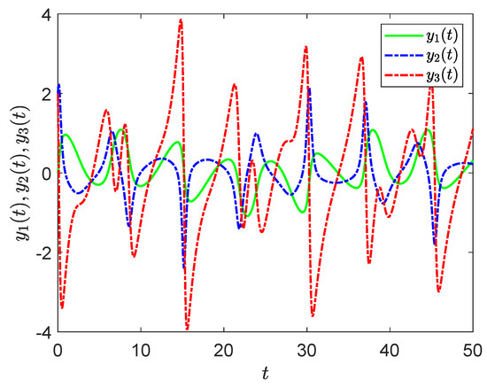
Figure 33. Solution profiles of the chaotic system.

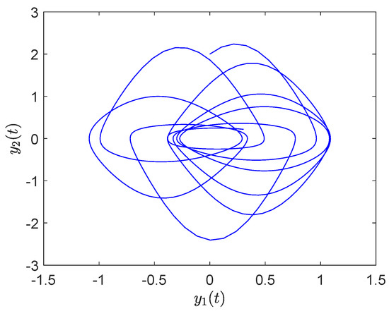
Figure 34. Phase portraits of $y_1$ and $y_2$.

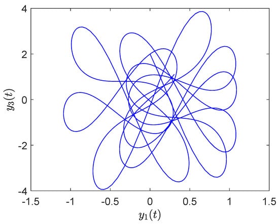
Figure 35. Phase portraits of $y_1$ and $y_3$.

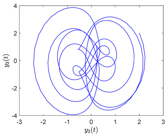
Figure 36. Phase portraits of $y_2$ and $y_3$.

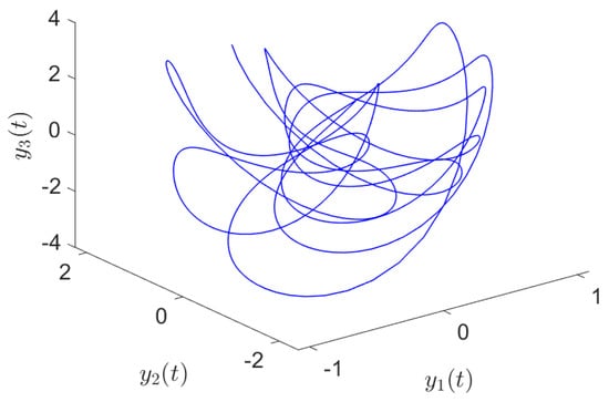
Figure 37. Phase portraits of $y_1$, $y_2$ and $y_3$.

3.3.4. Nonlinear Systems Example 4

Consequently, we demonstrate the applicability of the proposed method using the five-dimensional non-dissipative Lorenz model given as

$$\begin{array}{ccc}\hfill \dot{y_1}& =& \sigma (y_2-y_1),\hfill \\ \hfill \dot{y_2}& =& -y_1{y}_3+\rho y_1-y_2,\hfill \\ \hfill \dot{y_3}& =& y_1{y}_2-y_1{y}_4-b{y}_3,\hfill \\ \hfill \dot{y_4}& =& y_1{y}_3-2y_1{y}_5-c{y}_4,\hfill \\ \hfill \dot{y_5}& =& 2y_1{y}_4-4b{y}_5.\hfill \end{array}$$

(50)

Figure 38, Figure 39, Figure 40, Figure 41 and Figure 42 depict the errors, and we can clearly see that the level of accuracy for this proposed method is very high. The last few selected Figure 43, Figure 44, Figure 45, Figure 46, Figure 47, Figure 48, Figure 49, Figure 50, Figure 51, Figure 52, Figure 53 and Figure 54 display the selected phase portraits when varying the parameters.

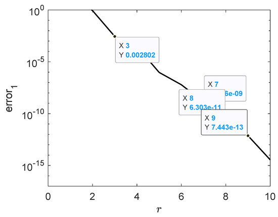
Figure 38. Convergence graph of $y_1$.

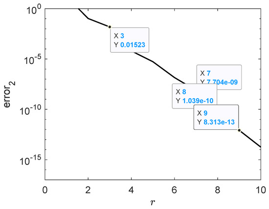
Figure 39. Convergence graph of $y_2$.

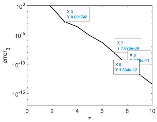
Figure 40. Convergence graph of $y_3$.

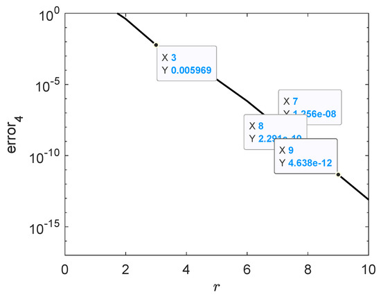
Figure 41. Convergence graph of $y_4$.

Figure 42. Convergence graph of $y_5$.

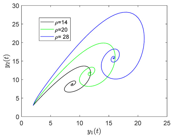
Figure 43. Phase portraits of $y_1$ and $y_2$ when varying $\rho$.

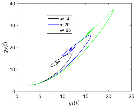
Figure 44. Phase portraits of $y_1$ and $y_3$ when varying $\rho$.

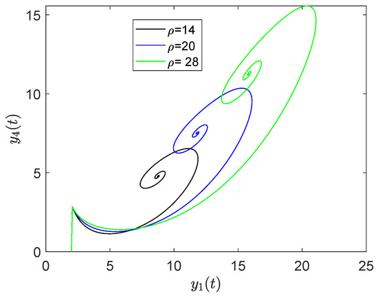
Figure 45. Phase portraits of $y_1$ and $y_4$ when varying $\rho$.

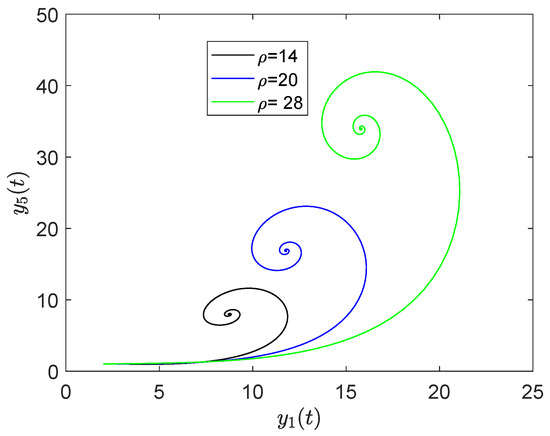
Figure 46. Phase portraits of $y_1$ and $y_5$ when varying $\rho$.

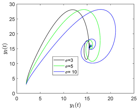
Figure 47. Phase portraits of $y_1$ and $y_2$ when varying $\sigma$.

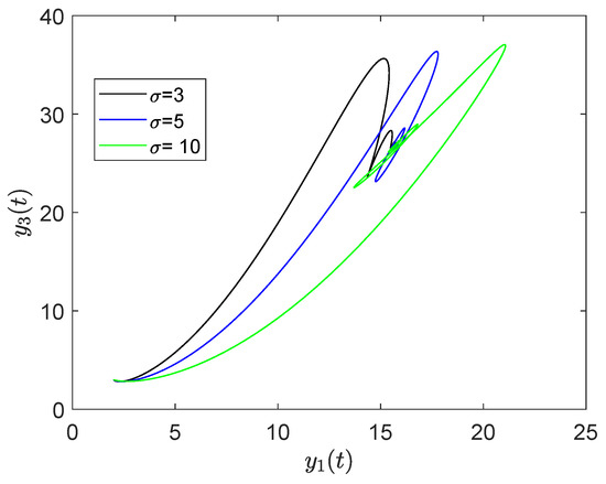
Figure 48. Phase portraits of $y_1$ and $y_3$ when varying $\sigma$.

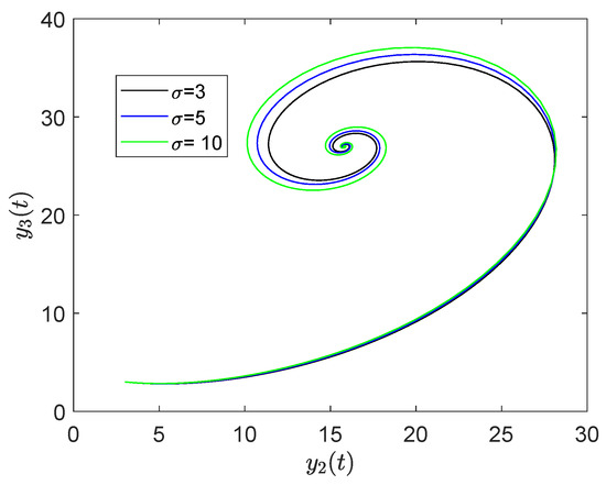
Figure 49. Phase portraits of $y_2$ and $y_3$ when varying $\sigma$.

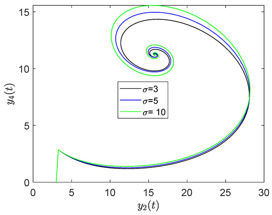
Figure 50. Phase portraits of $y_2$ and $y_4$ when varying $\sigma$.

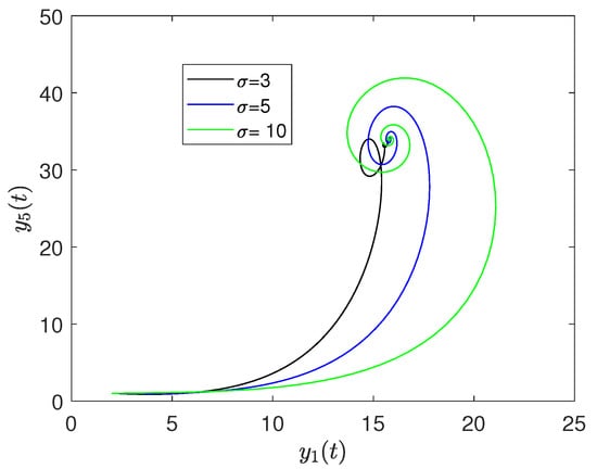
Figure 51. Phase portraits of $y_1$ and $y_5$ when varying $\sigma$.

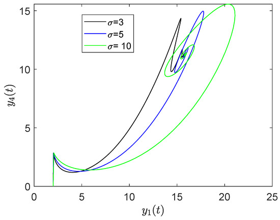
Figure 52. Phase portraits of $y_1$ and $y_4$ when varying $\sigma$.

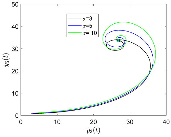
Figure 53. Phase portraits of $y_3$ and $y_5$ when varying $\sigma$.

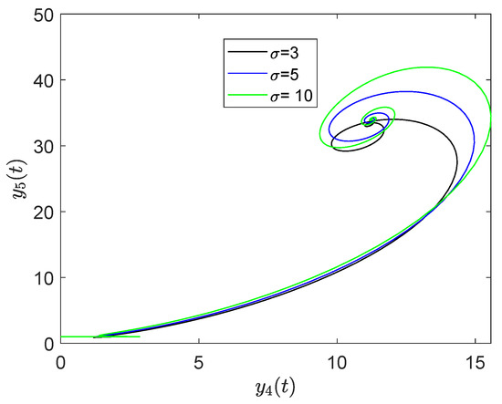
Figure 54. Phase portraits of $y_4$ and $y_5$ when varying $\sigma$.

4. Conclusions

This study proposed the application of newly developed block hybrid linear multi-step methods with off-step points for solving linear and nonlinear single and systems of differential equations. Numerical results for the current methods are excellent and compare very well with the exact solutions. The high levels of convergence indicate that the HBMs are very good candidates to solve high order systems of nonlinear systems of equations. We consequentially remark that the study observed that the numerical approximations converged quickly after very few iterations, even with very many collocation points and small step sizes. We also observed that the block hybrid methods are far superior to some classical numerical methods such as the Runge–Kutta methods. This great accuracies of the block hybrid methods and their user friendliness will go a long way in their applications in more complex models. Unfortunately, at the moment BHMs can only be applied to linear equations. Nonlinear equations have to be linearized first.

References

- Shampine, L.F.; Watts, H.A. Block Implicit One-Step Methods. Math. Comput. 1969, 23, 731–740. [Google Scholar] [CrossRef]
- Brugnano, L.; Trigiante, D. Solving Differential Problems by Multistep Initial and Boundary Value Methods; Gordon and Breach Science Publishers: Amsterdam, The Netherlands, 1998. [Google Scholar]
- Ramos, H.; Kalogiratou, Z.; Monovasilis, T.H.; Simos, T.E. An optimized two-step hybrid block method for solving general second order initial-value problems. Numer. Algorithms 2016, 72, 1089–1102. [Google Scholar] [CrossRef]
- Yap, L.K.; Ismail, F.; Senu, N. An Accurate Block Hybrid Collocation Method for Third Order Ordinary Differential Equations. J. Appl. Math. 2014, 2014, 549597. [Google Scholar] [CrossRef]
- Yap, L.K.; Ismail, F. Block Hybrid Collocation Method with Application to Fourth Order Differential Equations. Math. Probl. Eng. 2015, 2015, 561489. [Google Scholar] [CrossRef]
- Awari, Y.S. Some generalized two-step block hybrid Numerov method for solving general second order ordinary differential equations without predictors. Sci. World J. 2015, 12, 12–18. [Google Scholar]
- Albarbi, A.R.; Almatrafi, M.B. Exact and Numerical SolitaryWave Structures to the Variant Boussinesq System. Symmetry 2020, 12, 1473. [Google Scholar] [CrossRef]
- Xia, S. Existence of a weak solution to a generalized Riemanntype hydrodynamical equation. In Applicable Analysis; Taylor & Francis: Abingdon, UK, 2022. [Google Scholar] [CrossRef]
- Albarbi, A.R.; Almatrafi, M.B. Exact solitary wave and numerical solutions for geophysical KdV equation. J. King Saud Univ. Sci. 2022, 34, 102087. [Google Scholar] [CrossRef]
- Ononogbo, C.B.; Airemen, I.E.; Ezurike, U.J. Numerical Algorithm for One and Two-Step Hybrid Block Methods for the Solution of First Order Initial Value Problems in Ordinary Differential Equations. Appl. Eng. 2022, 6, 13–23. [Google Scholar] [CrossRef]
- Gear, C.N. Hybrid methods for initial value problems in Ordinary Differential Equations. SIAM J. Numer. Anal. 1964, 2, 69–86. [Google Scholar] [CrossRef]
- Motsa, S.S. Block hybrid methods. In Proceedings of the 13th Annual Workshop on Computational Mathematics and Modelling, University of KwaZulu-Natal, Pietermaritzburg Campus, Durban, South Africa, 5–9 July 1964. [Google Scholar]
- Yakubu, D.G.; Shokri, A.; Kumleng, G.M.; Marian, D. Second Derivative Block Hybrid Methods for the Numerical Integration of Differential Systems. Fractal Fract. 2022, 6, 386. [Google Scholar] [CrossRef]
- Ramos, H.; Rufai, M.A. A two-step hybrid block method with fourth derivatives for solving third-order boundary value problems. J. Comput. Appl. Math. 2022, 404, 113419. [Google Scholar] [CrossRef]
- Motsa, S. Overlapping Grid-Based Optimized Single-Step Hybrid Block Method for Solving First-Order Initial Value Problems. Algorithms 2022, 15, 427. [Google Scholar] [CrossRef]
- Burden, R.L.; Faires, J.D. Numerical Analysis, 9th ed.; Brooks/Cole, Cengage Learning: San Francisco, CA, USA, 2011; pp. 302–314. [Google Scholar]
- Motsa, S.S. Hybrid block methods for IVPs using Mathematica. In Proceedings of the 14th Annual Workshop on Computational Mathematics and Modelling, University of KwaZulu-Natal, Pietermaritzburg Campus, Durban, South Africa, 4–8 July 2022. [Google Scholar]
- Bellman, R.E.; Kalaba, R.E. Quasilinearization and Nonlinear Boundary-Value Problems; Elsevier: New York, NY, USA, 1965. [Google Scholar]
- Fang, H.P.; Hao, B.L. Symbolic dynamics of the Lorenz equations. Chaos Solitons Fractals 1966, 7, 217–246. [Google Scholar] [CrossRef]
- Hao, B.; Liu, J.; Zheng, W. Symbolic dynamics analysis of the Lorenz equations. Phys. Rev. 1998, 57, 5378. [Google Scholar] [CrossRef]
- Garashchuk, I.R.; Kudryashov, N.A.; Sinelshchikov, D.I. On the analytical properties and some exact solutions of the Glukhovsky-Dolzhansky system. J. Phys. Conf. Ser. 2017, 788, 012013. [Google Scholar] [CrossRef]
- Brogliato, B.; Lozano, R.; Maschke, B.; Egeland, O. Dissipative Systems Analysis and Control, 2nd ed.; Theory and Applications; Springer: London, UK, 2007. [Google Scholar]
Disclaimer/Publisher’s Note: The statements, opinions and data contained in all publications are solely those of the individual author(s) and contributor(s) and not of MDPI and/or the editor(s). MDPI and/or the editor(s) disclaim responsibility for any injury to people or property resulting from any ideas, methods, instructions or products referred to in the content. |
© 2023 by the author. Licensee MDPI, Basel, Switzerland. This article is an open access article distributed under the terms and conditions of the Creative Commons Attribution (CC BY) license (https://creativecommons.org/licenses/by/4.0/).