Abstract
In this paper, we present a study of the diffusion properties of a deterministic model for settling particles in two displacement dimensions. The particularities of the novel deterministic model include the generation of Brownian motion and a two-dimensional displacement model without stochastic processes, which are governed by a set of six differential equations. This model is a piecewise system consisting of subsystems governed by jerk equations. With this model, we can consider different conditions of diffusion in both the dimensions and size of the space where the particles are dispersed. The settling time versus the dispersion medium and its size, as well as the average settling time and its probability distributions, are analyzed. Furthermore, the probability distributions for the settling location are presented for the changes in the diffusion parameters and space size. Finally, the basins of attraction for the settling positions are shown as a function of each dimensional diffusion parameter and for the medium size.
MSC:
37N20; 70k99; 76R50; 37D05
1. Introduction
The study of particle propagation through hydrodynamic fluids is a topic that has attracted the attention of many research groups since the reported findings of Brown in 1828 [1]. The diffusion phenomenon has very important implications for real systems such as porous media [2,3], electrostatic interactions [4,5], liquid films [6,7], magnetic media [8,9], and biology [10], among others. On the other hand, the study of deterministic dissipative systems has become very important for facilitating the understanding of the particle dispersion process in a medium. In 1954, Lónvan Hove used quantum mechanical theory to study the transport process produced by a small perturbation as a characteristic property responsible for the diffusive effects in the evolution of the system, eliminating the need for assuming a random phase during consecutive short-time intervals [11]. One of the first publications on the deterministic behavior of particles was presented by Russo in [12], who used three different schemes (based on the approximation of the gradient on an irregular mesh and a finite-element approach) to study their convergence and proposed some applications for the Fokker–Plank equation and other problems of the disposing of particles. However, several approaches have since been presented that provide a better understanding, for instance, the deep origin of the stochastic nature of a dynamical system. Ford et al. Zwanzig, and Caldeira et al. [13,14,15] were the first to show that when starting with a Hamiltonian (deterministic) description of both the environment and system, random noise emerges once the environmental degrees of freedom are somehow eliminated. Recently, some works [16,17] have been undertaken to formalize Zwanzig’s approach and understand how to describe stochastic noise given the microscopic details of the environment. In addition, recent publications on the deterministic behavior of particles in a fluid have been presented by Trefàn et al. [18], where the results were obtained using a discrete system. Another ingenious proposal for approaching the deterministic Brownian motion in a one-dimensional displacement by demonstrating its statistical properties was presented by Huerta et al., where a continuous time system inspired by the jerk equation was used [19]. Furthermore, deterministic behavior has been theoretically established for both integer- and fractional-order derivatives [20,21,22].
The study of particle diffusion has been addressed in many areas since this paradigm constitutes the basis of numerous applications ranging from colloidal suspensions, emulsions, and simple polymeric solutions to biological systems, among others. Some examples are the diffusion of proteins and lipids [23,24], the transport of biological cells in crowded media, and the use of a generalized Langevin equation to describe the lateral diffusion of a protein in a lipid bilayer [25,26].
One of the most important areas in particle dispersion is pharmacology due to the interest in achieving more effective drug delivery with smaller doses [27]. Drugs are driven by physiological transport forces, mainly by solvent-driven flow (convection) but also by molecular agitation (diffusion). The appropriate combination of these two forces can determine the effective penetration and distribution of the substances in the arterial walls. The role of the convection and diffusion processes, along with the local flux conditions and characteristics of the drug and tissue, will determine the local drug distribution over space and time [28].
For drugs, the use of stochastic diffusion modeling approaches deserves consideration in model-informed drug discovery because it considers random events that can have a significant impact on treatment effects and disease progression, especially when the population size is small [29]. Furthermore, deterministic systems have the advantage of greater mathematical simplicity, are computationally less demanding than stochastic systems, and the parameter estimations are well-established, and a large toolkit is available to help with model fitting and simulation [29].
In this paper, a deterministic model for particle settling is presented, which is based on a deterministic model of Brownian motion. A two-dimensional model is constructed considering piecewise systems and the jerk equation, where each defined domain emulates a potential that can be modified by a single parameter related to the conditions of the medium. This model allows us to consider different diffusion conditions along each dimension in addition to the size of the dispersion medium. Its behavior is analyzed under different conditions. The generation of deterministic models, such as the proposed model, provides advantages over other approaches since a purely theoretical derivation, even in presence of a nonlinear coupling for particle interactions, is still a difficult task in terms of the mathematical definition for the friction and noise terms [14,17]. The rest of this paper is organized as follows. In Section 2, the basics of particles, the Langevin equation, and the construction of the model are presented. Section 3 contains the numerical results obtained using the proposed model in terms of the changes in the different parameters considered. The statistical analysis of the time series is presented in Section 4. Finally, the conclusions are drawn in Section 5.
2. Deterministic Model for Particle Settling
The onset of Brownian motion occurs when a particle is suspended in a fluid. The motion of this particle occurs due to collisions between the fluid molecules, with each collision causing a small change in velocity. This is because, under normal conditions, the suspended particle suffers about 10 collisions per second so the accumulated effect is substantial. Each of these collisions is determined by the previous event, which is produced by physical interactions within the system. Since it is thought that each collision produces a kink in the path of the particle, it is not possible to accurately follow the path as the details are infinitely complex. Thus, the Brownian particle makes a fluctuating movement. So, stochastic models of Brownian motion follow the average motion of a particle, rather than the particular path of a particle. The stochastic theory of Brownian motion of a free particle (in the absence of an external field of force) is generally governed by the Langevin equation as follows:
where x and v denote the particle position and velocity, respectively. According to Equation (1), the influence of the surrounding medium on particle motion can be split into two parts. The first term stands for the friction applied to the particle. It is assumed that the friction term used is according to Stokes’ law, which states that the friction force decelerates a spherical particle of radius a and mass m. Hence, the friction coefficient is given as follows:
where denotes the viscosity of the surrounding fluid. The second term is the fluctuation acceleration, which provides the stochastic character of the motion and depends on the fluctuation force as , where m is the particle mass. Two principal assumptions were made about the stochastic term in order to produce Brownian motion:
- is independent of x and v.
- varies much faster than v.
The latter assumption is that there exists a time interval during which the variations in v are very small. Alternatively, we may say that although and are expected to differ by a negligible amount, no correlation between and exists as it is a stochastic term.
In order to generate a deterministic model of Brownian motion, an additional freedom degree is added to the system in (1). Moreover, the stochastic term is avoided by replacing the fluctuating acceleration with the jerk equation. The class of affine linear systems considered here presents oscillations (a "one-spiral" trajectory called a scroll) around equilibria due to stable and unstable manifolds. This is reached if the linear part of the system has a saddle equilibrium point.
To generate deterministic Brownian motion, the stochastic term is replaced with a new variable z, which is defined by a third-order differential equation, and a Brownian motion based on the jerk equation that was reported in [19], which we call jerk-based Brownian motion. The proposed variable z acts as a fluctuating acceleration and produces a deterministic dynamical motion without a stochastic term. Its behavior presents the statistical features of Brownian motion, as demonstrated in a previous work [18]. However, in the jerk-based Brownian motion model, the fluctuation acceleration has a direct dependence on the position, velocity, and acceleration due to the jerky equation involved [19]. When a particle moves in a fluid, the friction and collisions with other particles that exist in the medium produce changes in the speed and acceleration of the movement; these changes are considered in the jerky equation (which is usually considered in stochastic terms). The model based on an unstable dissipative system (UDS) [30,31,32] in one dimension is defined as follows:
where are constant parameters, with , and acts as a constant piecewise function, i.e., a step function.
The term is driven by a switching law (SW), which is given by a piecewise function that commutes in the space where the particle crosses a switching surface (SS). There are many switching surfaces that are defined by planes perpendicular to the x-axis. Thus, domains are demarcated by these SSs, which are considered the edges of each domain. In the case of real systems, domains can be seen as having multi-well potential with a short fluctuation escape time, where each domain is defined by SSs that retain their unstable behavior according to the linear part of the system. When a particle moves in a fluid, changes in the speed and acceleration of its movement occur due to friction and collisions with other particles that exist in the environment. These changes are considered in the unequal equation. The SS delimits each region of potential, and when a particle crosses the surface, it represents a change in the particle’s potential, i.e., a collision with other medium particles. The parameter is defined as follows:
where are parameters. The function is defined as follows:
Without loss of generality and in the same spirit of the one-dimensional displacement model, we construct our two-dimensional displacement model considering the boundary conditions, i.e., settlement conditions, in one of the displacement dimensions. The deterministic model is a jerk-based Brownian motion system that is defined by the following two-dimensional displacement system:
where and are state vectors, and b(x) and b(y) are driven by the round function given in (4). Note that the dynamic of each dimension is governed by Equation (3). Let be a matrix with real coefficients defined by , and the linear operator is given by
where are real constants that guarantee unstable behavior, with , and K is a single parameter that allows us to consider the changes in the type of medium. This is because different behaviors are obtained by the changes in the bifurcation parameter K, which correlate directly with the direction and location of their stable and unstable manifolds, as well as the values of their eigenvalues [33], and can be understood as the ability of the particle to cross over to the next domain. It is worth mentioning that the deterministic model (6) is a two-dimensional displacement jerk-based Brownian model and its dynamics evolve in a six-dimensional space. Then, the proposed bidimensional model considering the edge conditions is defined as follows:
where k is a parameter that makes an attractive equilibrium point, and determine different diffusion conditions for each dimension, , , and m is the parameter used to define the space size where the model is defined.
3. Numerical Results of Time Settling of Particles
The study of the settling time of particles in two-dimensional displacement is realized by the proposed deterministic model (8). To carry out the numerical analysis of the proposed model, the following parameters are used with the fourth-order Runge–Kutta method: , , , , , and . The parameters were selected in such a way that the conditions of a UDS type I system are met, following the methodology proposed in Ref. [32], via numerical exploration to guarantee that when the trajectory reaches the SS, the probability of crossing to the next domain is . In terms of the settlement case, let us begin by showing some examples of the dynamics found in the trajectory of a particle in a two-dimensional displacement system for different sets of parameters.
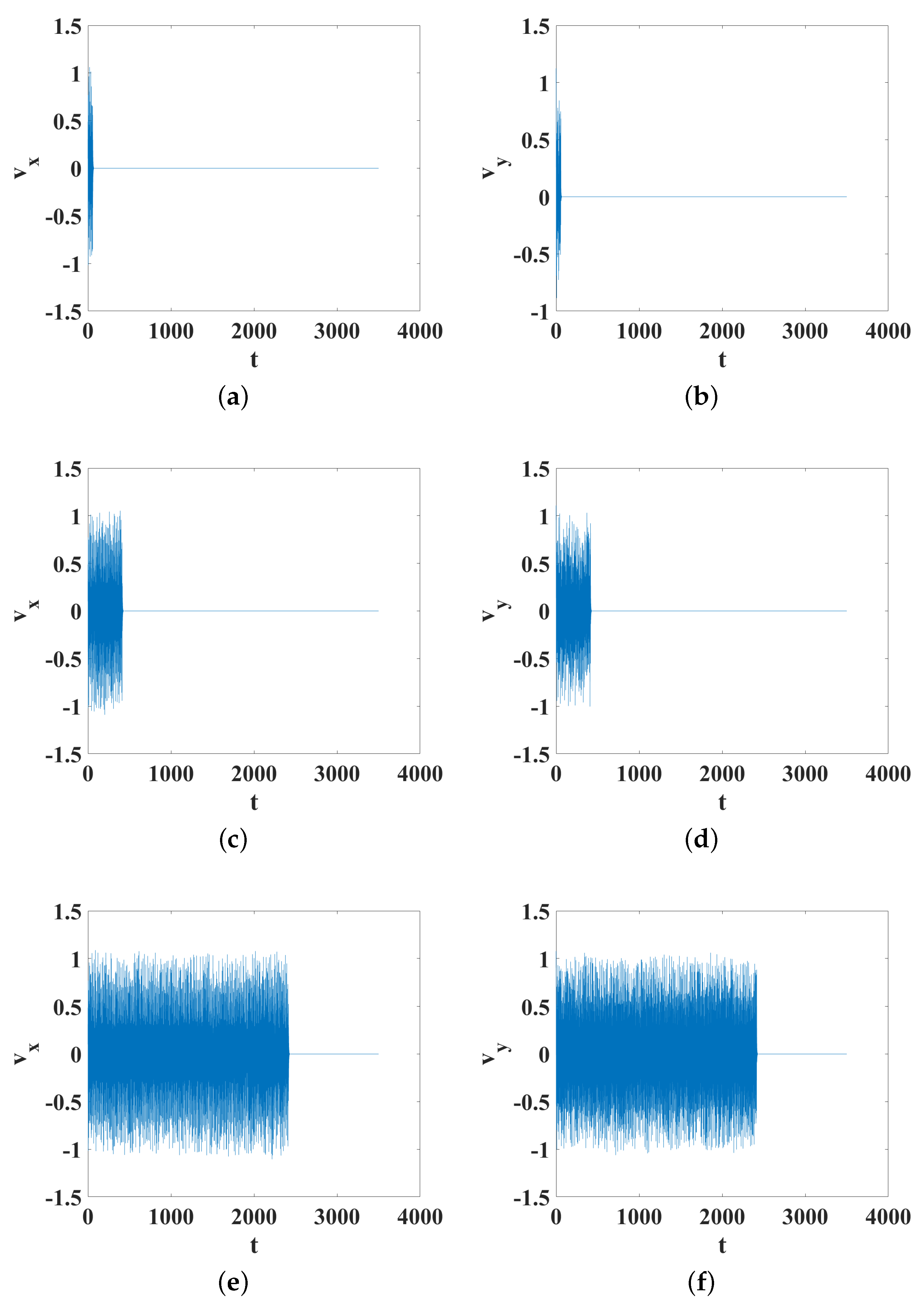
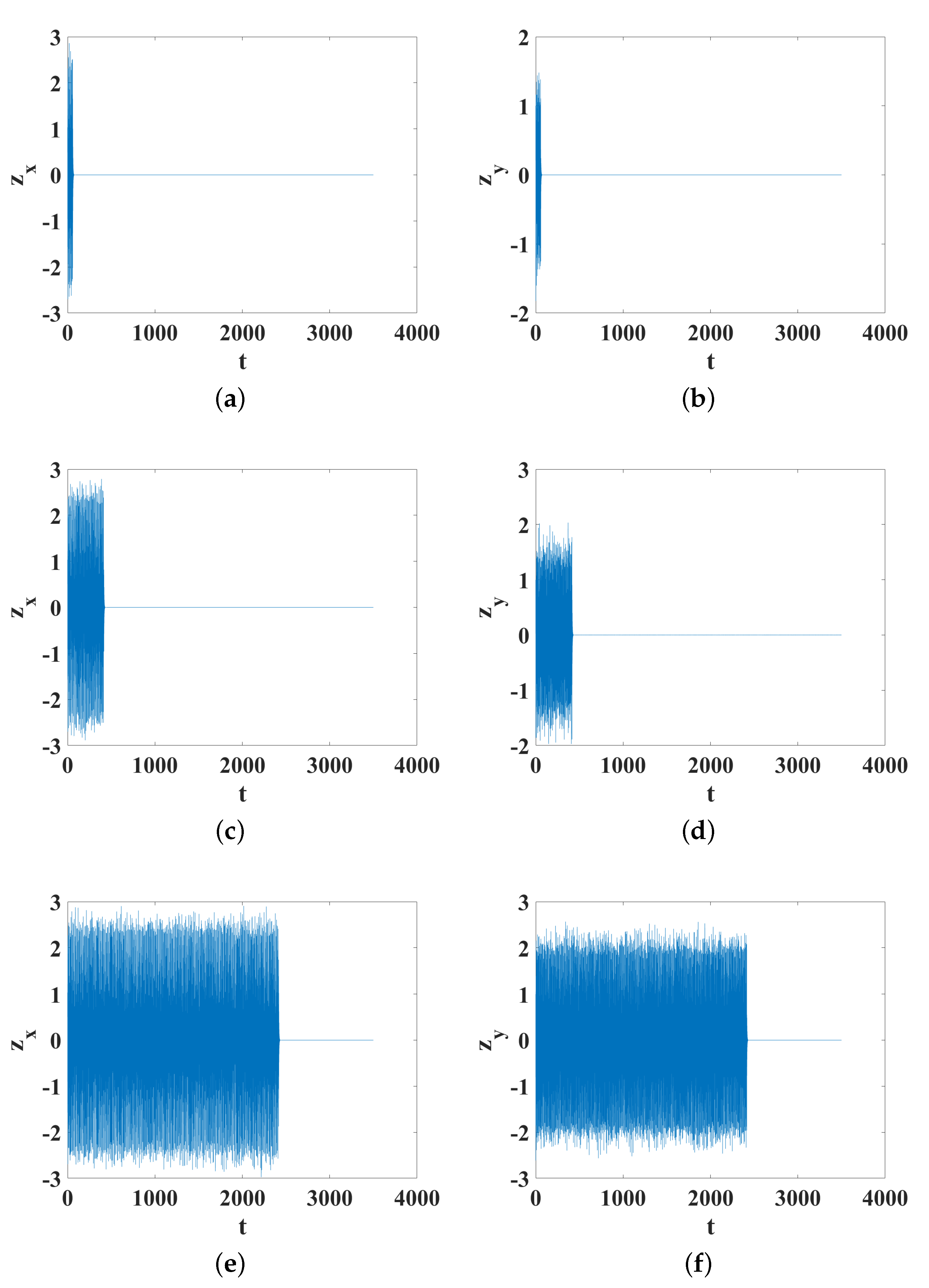
Figure 1 shows the analysis of the trajectory of a particle for a fixed initial condition and different values of the parameter ∈ [0.6, 1.8]. The other parameters are , , and .
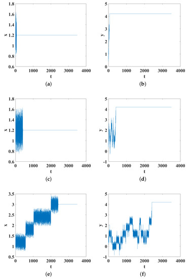
Figure 1.
Times of particle settling for different initial conditions and a single value of the dispersion medium (). (a,b) ; (c,d) ; (e,f) .
We only show three values of the parameter = 0.6, 0.7, and 1.0, to illustrate the behavior of the particle. The first column in Figure 1 shows the x-position versus the settling time for the different values of the parameter . Figure 1a corresponds to = 0.6 and we can observe that the particle quickly converges to a steady state. When the value of the parameter increases to 0.7, the particle converges to a steady state in about 500 arbitrary units (A.U.) of time (see Figure 1c). If the value of the parameter continues to increase, for example, to , the particle oscillates more before converging to a steady state (see Figure 1d) and the trajectory tends toward a Brownian movement as the parameter increases. The second column in Figure 1 shows the relationship between the position in y and the settling time, where it can be observed that for a fixed value of the dispersion medium size, the settling time for y increases as the parameter increases. Additionally, in Figure 2 and Figure 3, the velocity and acceleration versus time are shown, where we can observe that this variable remains bound for the parameter changes.
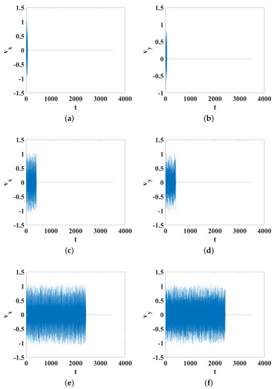
Figure 2.
Velocity time evolution for a fixed initial condition and different values of the dispersion medium (). (a,b) ; (c,d) ; (e,f) .
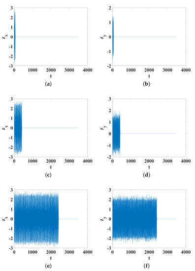
Figure 3.
Accelerations , versus time evolution for a fixed initial condition and different values of the dispersion medium (). (a,b) ; (c,(d) ; (e,f) .
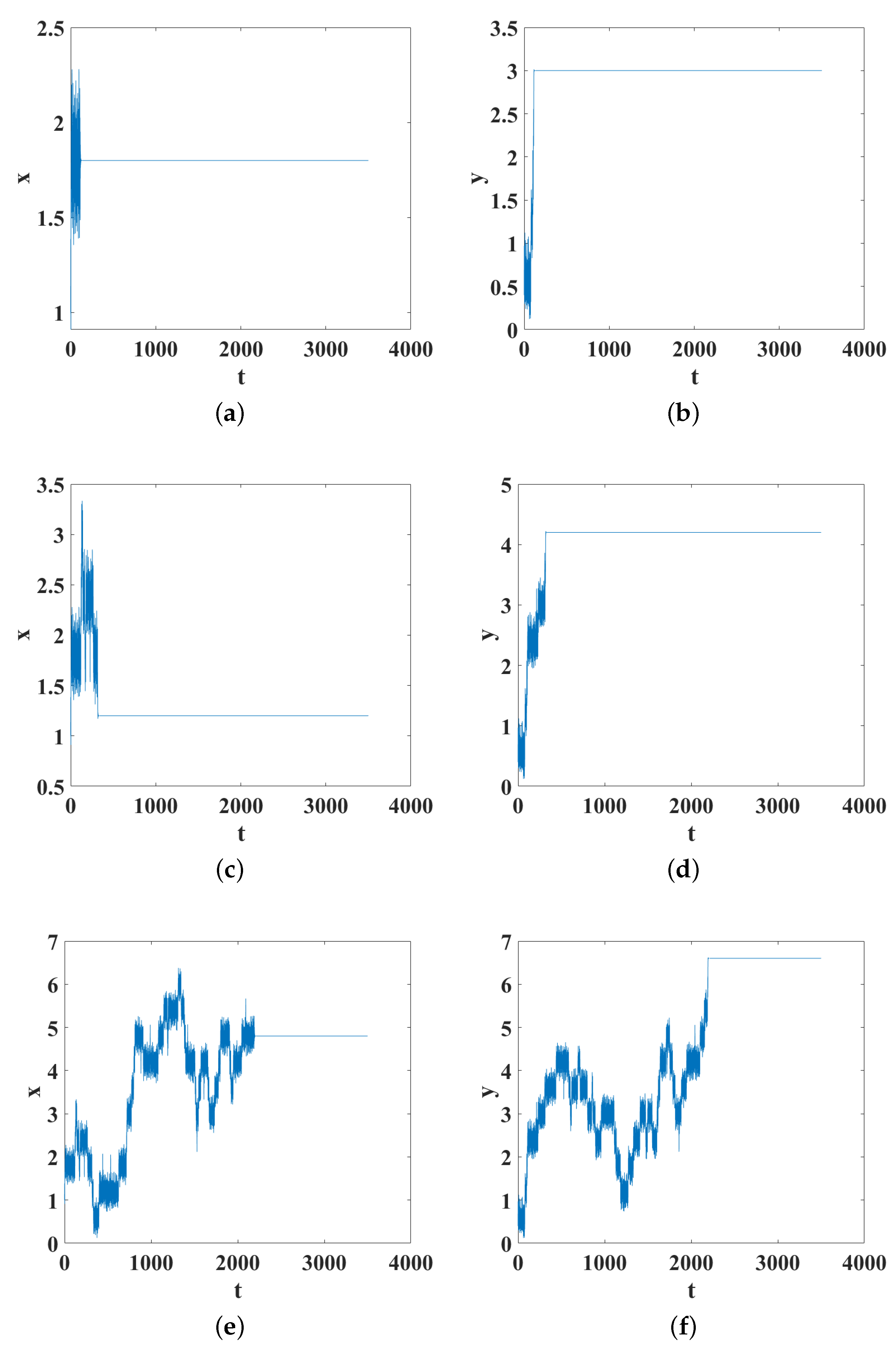
The second case that is analyzed corresponds to changing the value of the parameter and maintaining the value of the other parameter, that is, 0.6, 1.1, and 1.4. The other parameters are , , and . The initial condition for all the values of is fixed to . The first column in Figure 4 shows the relationship between the position in x and the settling time. Figure 4a corresponds to the case , where the particle reaches the edge in about 2200 A.U. of time. Figure 4c corresponds to the case , where the particle reaches the edge in about 2600 A.U. of time. However, when we continue to increase the value of , the settling time decreases, as shown in Figure 4e, which corresponds to the case , where we can observe that the particle reaches the edge in about 1800 A.U. of time. In contrast to the previous case where the settling time increased as the parameter increased, for this variation of , this does not occur.
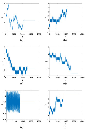
Figure 4.
Times of particle settling for different initial conditions and a single value of the dispersion medium size (). (a,b) ; (c,d) ; (e,f) .
The second column in Figure 4 shows the relationship between the position in y and the settling time that it takes to reach the edge for each value of the parameter , where, unlike the first case, the deposit time does not depend on the value of .
The final case to be analyzed corresponds to the behavior of the particle trajectory and the settling time when the size of the dispersion medium (m parameter) changes. As in the previous cases, the initial condition was fixed to for all cases, and we calculate how long it takes the particle to reach the edge for each value of the parameter m. The considered values of the parameter m are 4, 6, and 10, and the other parameters are , , and .
The first column in Figure 5 shows the trajectory of the particle in x versus the time in A.U. of time. In Figure 5a, we can observe that the particle quickly converges to a steady state for a small value of m = 4. When m increases to 6, it takes longer for the particle to reach a steady state (see Figure 5c). If we continue to increase the value of , the settling time increases (see Figure 5e). Therefore, the particle starts to oscillate with Brownian motion when the value of m increases. The second column in Figure 5 shows the trajectory of the particle in y versus the time in A.U. of time. The behavior at y agrees with the behavior at x, that is, an increase in the settlement time of the particle at the edge as the size of the dispersion medium increases.
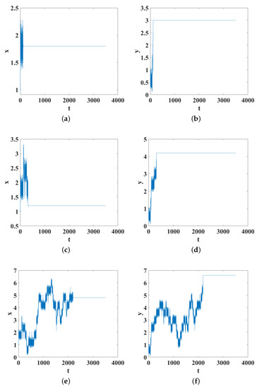
Figure 5.
Times of particle settling for a fixed initial condition and different values of the dispersion medium size. (a,b) ; (c,d) ; (e,f) .
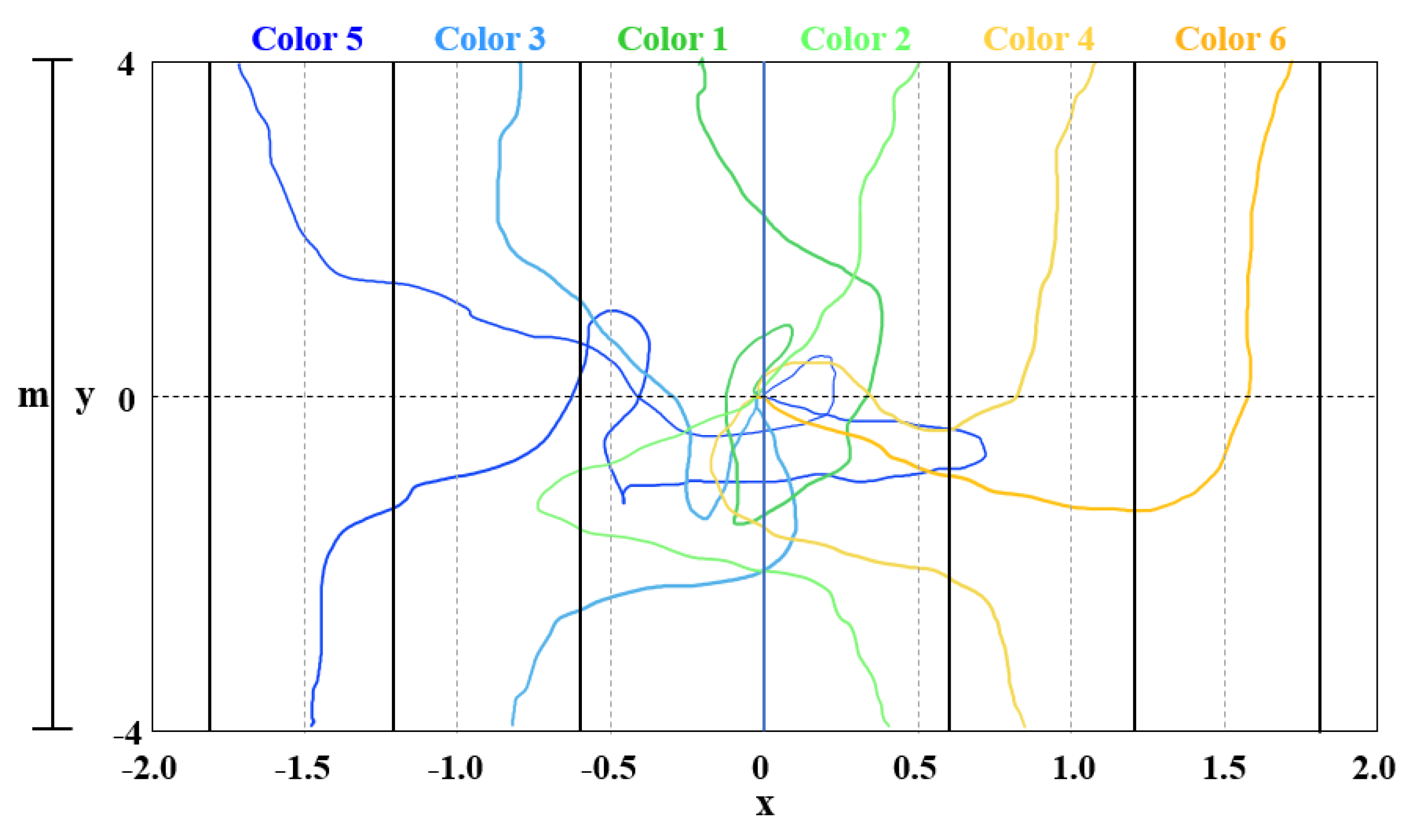
In Figure 6, the settlement of the particles at the edge of the dispersion medium is shown on a color map. The colors correspond to the final positions of the particle along the x-axis for a fixed initial condition and size of the dispersion medium (m), and the other parameters previously analyzed are varied. The region of color with the highest trend determines the point of attraction of the system.
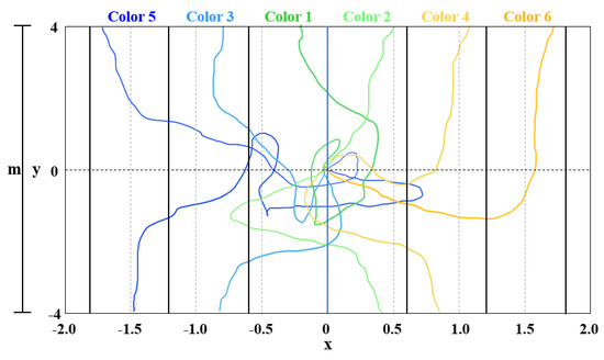
Figure 6.
Projections of the switching surfaces perpendicular to the plane (x,y) (black lines). Each colored line depicts the trajectory of a particle that moves along the two-dimensional plane (x,y) due to small changes in the initial conditions. The switching surfaces delimit each potential region that contains a settling point and when the particle crosses it, it represents a potential change in the particle.
4. Statistical Properties of Settling Model
In order to understand the phenomenon and visualize the dynamical changes induced for each system parameter, we numerically investigate the long-term behavior of the solutions to Equation (8). With the temporal series obtained for the cases mentioned in the previous section, we analyzed the time it takes for the particle to reach its destination and the location where it settles. By considering the different parameters , , and m, as well as the values of the parameters defined in the previous section, the statistical properties obtained for the time series are presented in this section. The first analysis carried out consisted of identifying the relationship between the settlement time and the parameter. For this, a fixed initial condition was considered and the time it takes to reach the edge was obtained for each value of the parameter . This can be seen in Figure 7, where the settling time shows an exponential trend as the parameter increases.
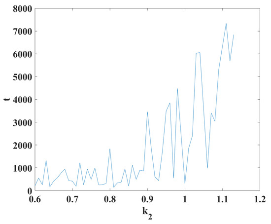
Figure 7.
Times of particle settling for a fixed initial condition with respect to the y diffusion parameter.
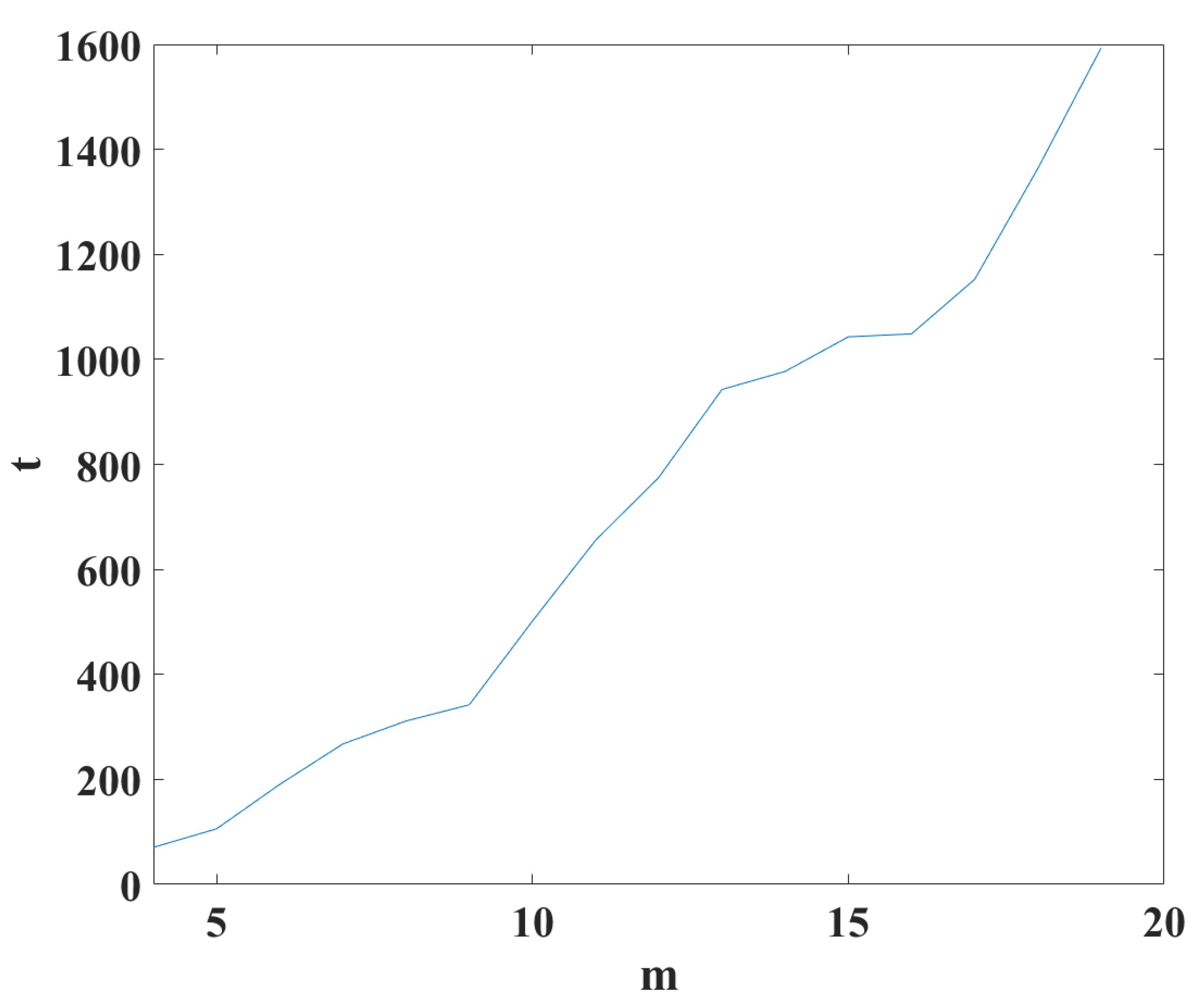
Another analysis was performed of the settlement time behavior with respect to the space size (m parameter), as in the previous case, a fixed initial condition was considered and the time it takes to reach the edge was obtained for each value of the parameter m. Figure 8 shows the parabolic growth with respect to m, which shows how the size of the space where the particles disperse has an important impact on the particle settling time.
Figure 8.
Times of particle settling for a fixed initial condition with respect to the space size m.
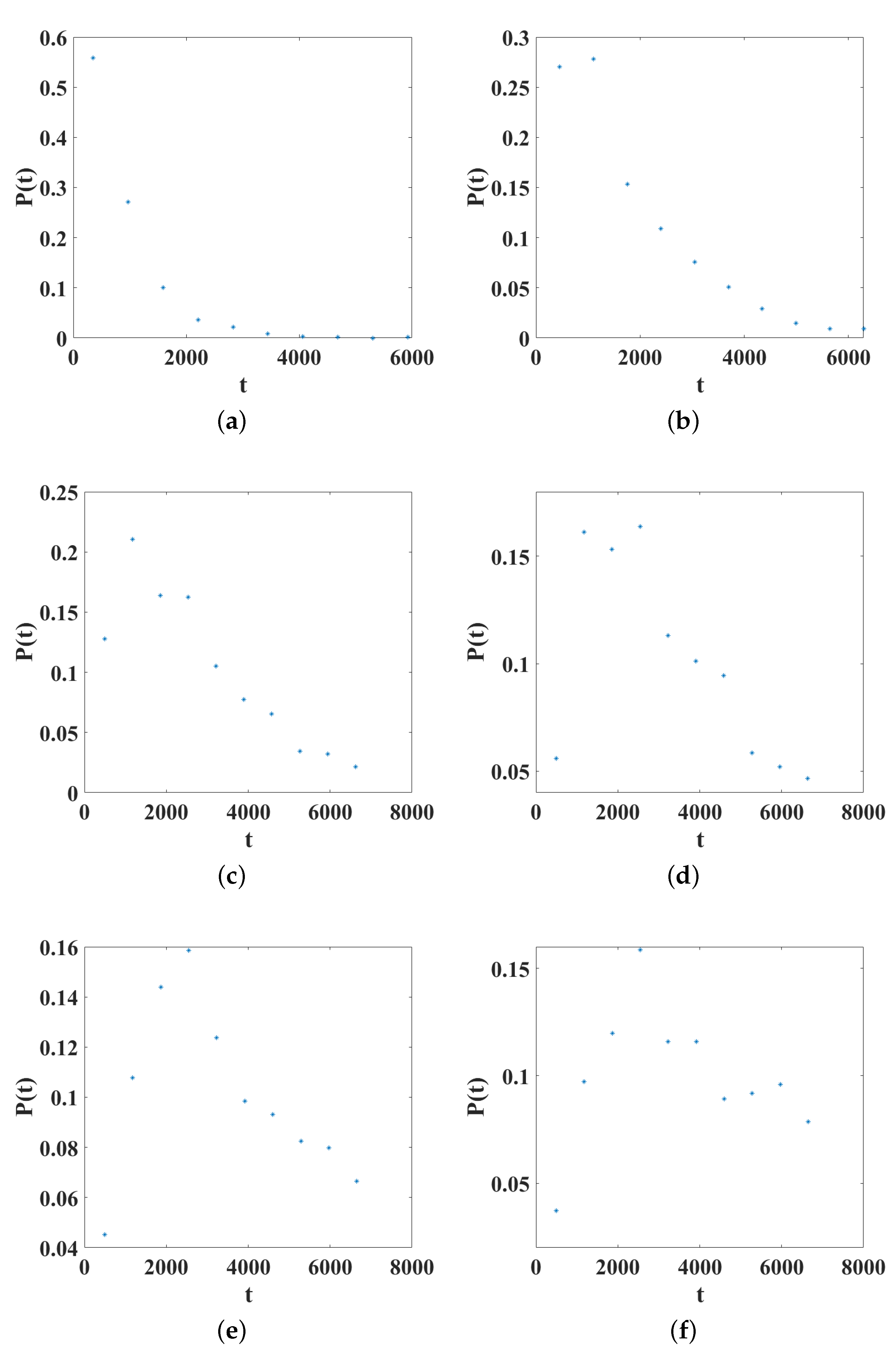
To generalize the behavior of the settlement time with respect to m and for a specific initial condition, we analyzed the time distribution for a set of 150 initial conditions. For this, we analyzed, in particular, a variation of in a range of and . The settlement times are organized in ten sets of the same length and the probability of occurrence is estimated. Figure 9 shows the time probability distribution for different values of with an increment of two units and . In this case, it can be seen that the probability distribution transitions from an exponential distribution to a uniform distribution as m increases.
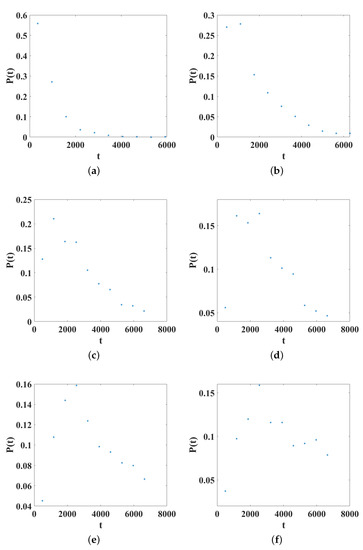
Figure 9.
Time probability distributions considering different initial conditions , for different values of m. (a) ; (b) ; (c) ; (d) ; (e) ; (f) .
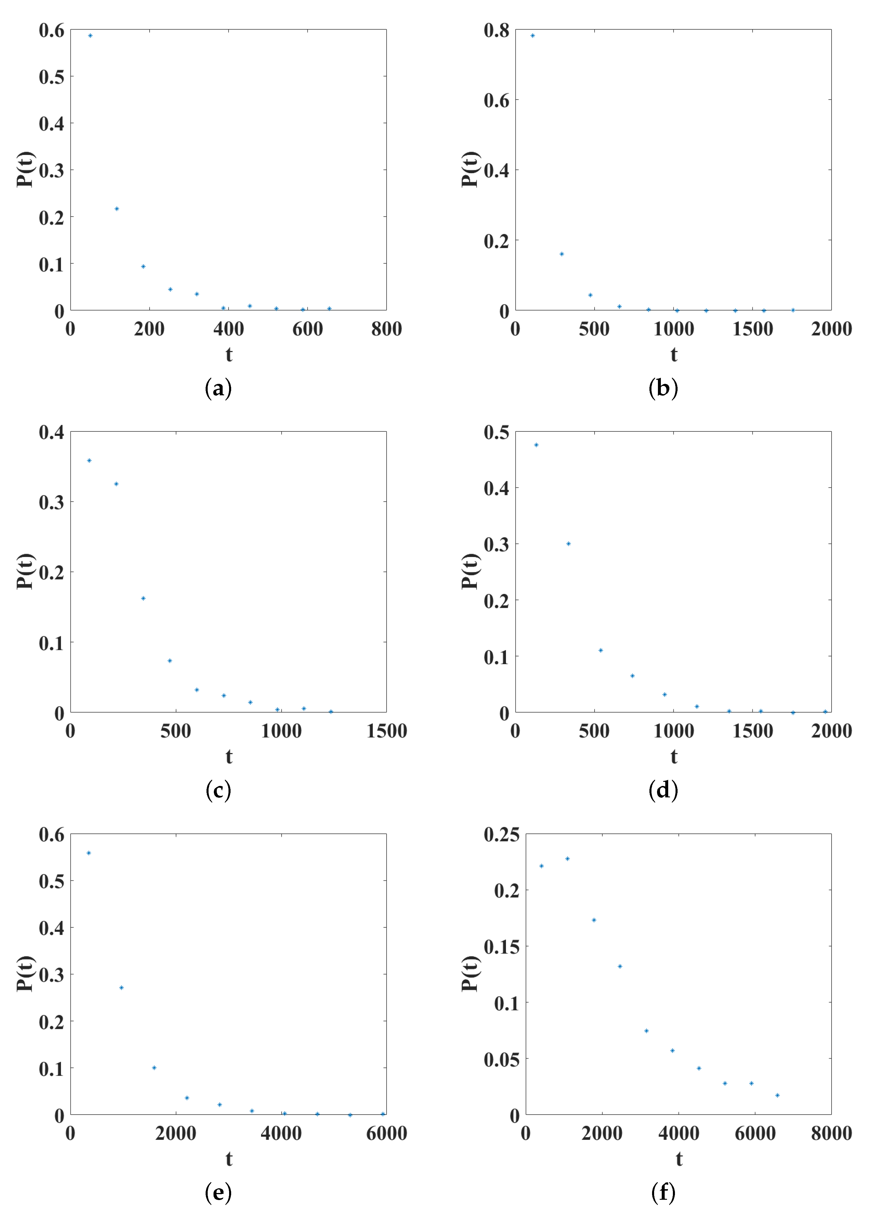
Additionally, the probability distribution of the settlement time from the changes in was analyzed for and . In Figure 10, we show the probability distributions for the same set of 150 initial conditions, where it can be observed that the shape of the distributions has the form of an exponential for small values of , and as increases, the distribution converges to a Gamma distribution.

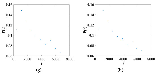
Figure 10.
Probability distributions of time settling with changes in . (a) ; (b) ; (c) ; (d) ; (e) ; (f) ; (g) ; (h) .
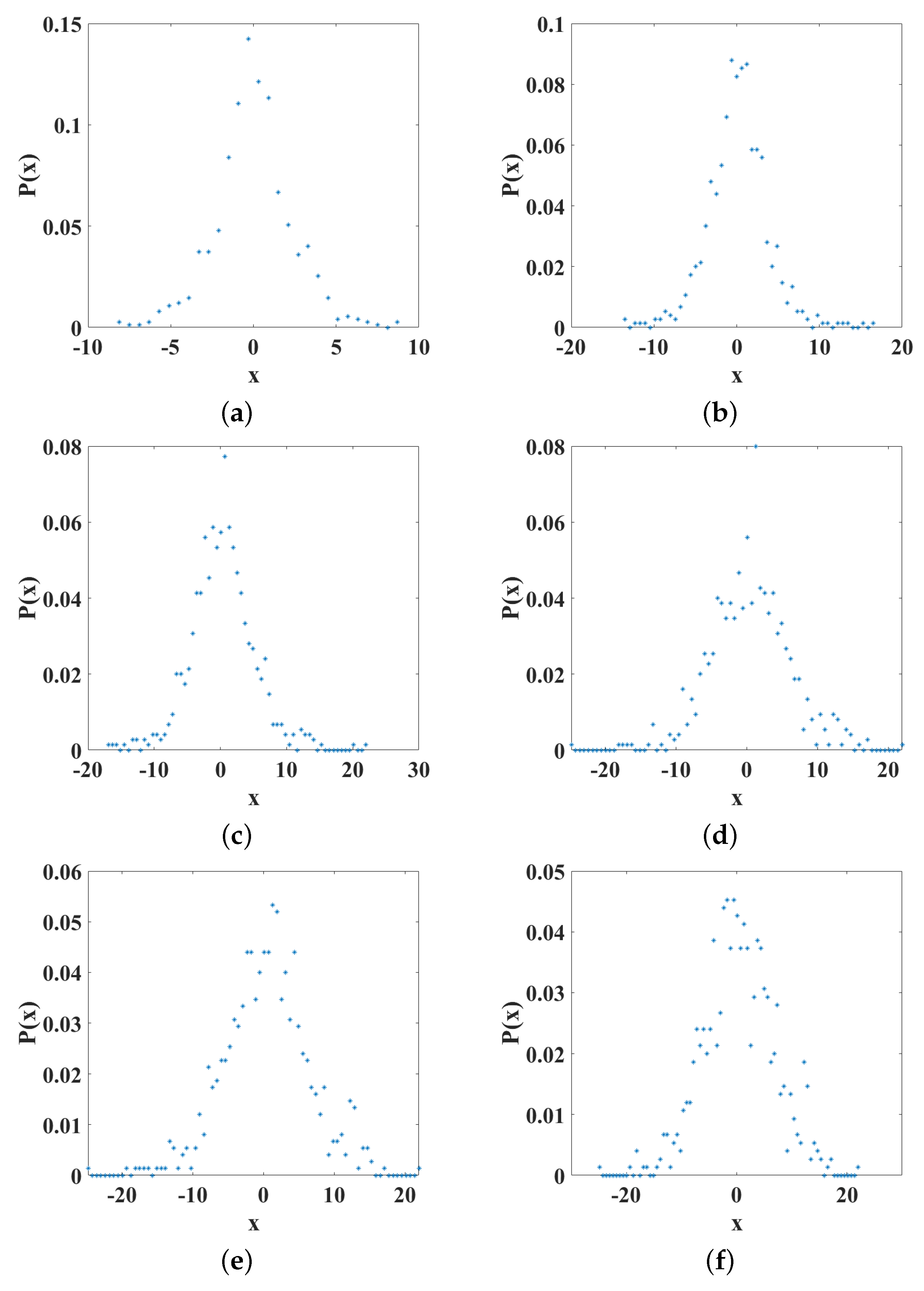
Regarding the settlement positions, similar to the analysis of time, we considered the same set of initial conditions as the changes in the particle’s final location. In this analysis, we considered the frequency of occurrence of each settlement location defined by the system in Equation (8), and then estimated the probability of occurrence. First, we analyzed the changes related to m in the range of with increments of 2 and . In Figure 11, the probability distributions are shown for the different values of m, where it can be seen that the shapes of the distributions are preserved. However, it is important to note that the maximum value of the probability decreases as m increases and the tails of the distribution are larger. This means that for larger values of m, it is possible to reach positions further away in the x-direction. Furthermore, the settlement positions were analyzed with respect to the parameter and the changes considered in the range of with increments of , with and . In Figure 12, the probability distributions are shown for the different values of , where it can be seen that the shapes of the distributions are preserved. Nevertheless, in contrast with the behavior observed for m, in this case, the maximum value of the probability increases as increases and the tails of the distribution are shorter. This means that for larger values of , the positions reached on the x-axis are less far-reaching.
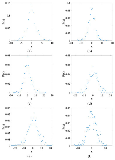
Figure 11.
Probability distributions of settling location with changes in m. (a) ; (b) ; (c) ; (d) ; (e) ; (f) .
Figure 12.
Probability distributions of settling location with changes in . (a) ; (b) ; (c) ; (d) ; (e) ; (f) ; (g) ; (h) .
Finally, color maps of the settlement positions for the considered initial condition with changes in , m, and are shown in Figure 13, Figure 14, and Figure 15, respectively. The values of the color bars represent the final positions along the x-axis. Figure 13 shows that for small values of , the solutions converge to a specific region around the origin, and as increases, the final locations no longer present a pattern that can be considered random. Figure 14 shows that the convergence region of the solutions is maintained for each initial condition regardless of the value of m (vertical changes). However, if the behavior is viewed horizontally, it can be seen that for large values of m, the final positions show random behavior. Regarding the changes in , Figure 15 shows that for the largest values of , the solutions converge to a specific region around the origin, and as decreases, the final locations no longer present a pattern that can be considered random, in contrast to that observed for in Figure 13.
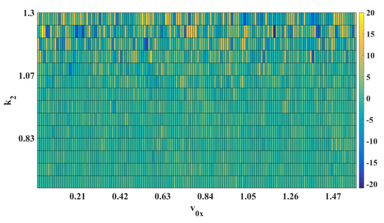
Figure 13.
Basin of attraction of settling locations for with changes in .
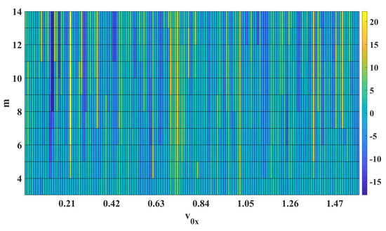
Figure 14.
Basin of attraction of settling locations for with changes in m.
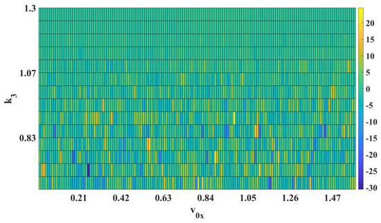
Figure 15.
Basin of attraction of settling locations for with changes in .
5. Conclusions
A deterministic dynamical system for settling particles that displays time series with Brownian motion properties has been presented. This model considers a two-dimensional diffusion process, as well as parameters that allow the modification of different medium conditions in each dimension. Additionally, a parameter was included to account for different space sizes. The statistical properties analyzed showed a parabolic growth in the deposit time with respect to the distance traveled, which is in accordance with random walk theory, and exponential growth with respect to the diffusion parameters. Regarding the settlement positions, we observed that by varying and , it was possible to control the directions in which the particles were dispersed. For small values of , displacement along the y-axis was favored, and for large values, displacement along the x-axis was favored. On the contrary, for small values of , displacement along the x-axis was favored, and for large values, displacement along the y-axis was favored. Finally, we observed that the changes in the settling locations with respect to the space size m remained practically unchanged, with the principal effect of this parameter being the time of deposition. Based on these results, which were obtained using an unstable piecewise system, it is believed that the methodology presented in this work can be applied to construct appropriate models using real experimental time series to study the spread of particles in pharmacology and consider different transport phenomena. Furthermore, the methodology can be used to determine the types of diffusions that occur with parameter changes, the types of correlations in the generated time series, and the effect of the parameters on the statistical properties of the displacement.
Author Contributions
S.E.V.P.: Writing—Original Draft, Writing—Review and Editing, Methodology, Software, Validation, Visualization. H.E.G.V.: Supervision, Writing—Review and Editing, Conceptualization, Resources, Project administration, Formal analysis, Writing—Review and Editing. G.H.C.: Formal analysis, Funding acquisition, Writing—Review and Editing. E.C.-C.: Supervision, Writing—Review and Editing, Conceptualization, Resources, Project administration. All authors have read and agreed to the published version of the manuscript.
Funding
This research received no external funding.
Data Availability Statement
Not applicable.
Acknowledgments
Eric Campos-Cantón acknowledges CONACYT for the financial support through Project no. A1-S-30433.
Conflicts of Interest
The authors declare no conflict of interest.
References
- Brown, R. A Brief Account of Microscopical Observations Made … on the Particles Contained in the Pollen of Plants, and on the General Existence of Active Molecules in Organic and Inorganic Bodies; Cambridge University Press: Cambridge, UK, 1828. [Google Scholar]
- Dagan, G. Theory of Solute Transport by Groundwater. Annu. Rev. Fluid Mech. 1987, 19, 183–213. [Google Scholar] [CrossRef]
- Tartakovsky, D.M.; Dentz, M. Diffusion in Porous Media: Phenomena and Mechanisms. Transp. Porous Media 2019, 130, 105–127. [Google Scholar] [CrossRef]
- Stylianopoulos, T.; Poh, M.-Z.; Insin, N.; Bawendi, M.G.; Fukumura, D.; Munn, L.L.; Jain, R.K. Diffusion of Particles in the Extracellular Matrix: The Effect of Repulsive Electrostatic Interactions. Biophys. J. 2010, 99, 1342–1349. [Google Scholar] [CrossRef] [PubMed]
- Dong, M.; Zhou, F.; Zhang, Y.; Shang, Y.; Li, S. Numerical study on fine-particle charging and transport behaviour in electrostatic precipitators. Powder Technol. 2018, 330, 210–218. [Google Scholar] [CrossRef]
- Cheung, C.; Hwang, Y.H.; Wu, X.-L.; Choi, H.J. Diffusion of Particles in Free-Standing Liquid Films. Phys. Rev. Lett. 1996, 76, 2531–2534. [Google Scholar] [CrossRef]
- Zhou, S.; Hwang, B.C.H.; Lakey, P.S.J.; Zuend, A.; Abbatt, J.P.D.; Shiraiwa, M. Multiphase reactivity of polycyclic aromatic hydrocarbons is driven by phase separation and diffusion limitations. Proc. Natl. Acad. Sci. USA 2019, 116, 11658–11663. [Google Scholar] [CrossRef]
- Pshenichnikov, A.F.; Elfimova, E.; Ivanov, A. Magnetophoresis, sedimentation, and diffusion of particles in concentrated magnetic fluids. J. Chem. Phys. 2011, 134, 184508. [Google Scholar] [CrossRef]
- Liu, Z.; He, J.; Ramanujan, R.V. Significant progress of grain boundary diffusion process for cost-effective rare earth permanent magnets: A review. Mater. Des. 2021, 209, 110004. [Google Scholar] [CrossRef]
- Coccia, M. Factors determining the diffusion of COVID-19 and suggested strategy to prevent future accelerated viral infectivity similar to COVID. Sci. Total. Environ. 2020, 729, 138474. [Google Scholar] [CrossRef]
- van Hove, L. Quantum-mechanical perturbations giving rise to a statistical transport equation. Physica 1954, 21, 517–540. [Google Scholar] [CrossRef]
- Russo, G. Deterministic diffusion of particles. Commun. Pure Appl. Math. 1990, 43, 697–733. [Google Scholar] [CrossRef]
- Ford, G.W.; Kac, M.; Mazur, P. Statistical Mechanics of Assemblies of Coupled Oscillators. J. Math. Phys. 1965, 6, 504–515. [Google Scholar] [CrossRef]
- Zwanzig, R. Nonlinear generalized Langevin equations. J. Stat. Phys. 1973, 9, 215–220. [Google Scholar] [CrossRef]
- Caldeira, A.O.; Leggett, A.J. Path integral approach to quantum Brownian motion. Phys. A Stat. Mech. Its Appl. 1983, 121, 587–616. [Google Scholar] [CrossRef]
- Hoel, H.; Szepessy, A. Classical Langevin dynamics derived from quantum mechanics. Discret. Contin. Dyn. Syst.- B 2020, 25, 4001–4038. [Google Scholar] [CrossRef]
- Di Cairano, L. On the derivation of a nonlinear generalized Langevin equation. J. Phys. Commun. 2021, 6, 015002. [Google Scholar] [CrossRef]
- Trefán, G.; Grigolini, P.; West, B.J. Deterministic Brownian motion. Phys. Rev. A 1992, 45, 1249–1252. [Google Scholar] [CrossRef]
- Huerta-Cuellar, G.; Jimenez-Lopez, E.; Campos-Cantón, E.; Pisarchik, A. An approach to generate deterministic Brownian motion. Commun. Nonlinear Sci. Numer. Simul. 2014, 19, 2740–2746. [Google Scholar] [CrossRef]
- Gilardi-Velázquez, H.E.; Campos-Cantón, E. Nonclassical point of view of the Brownian motion generation via fractional deterministic model. Int. J. Mod. Phys. C 2018, 29, 1850020. [Google Scholar] [CrossRef]
- Prada, D.; Herrera-Jaramillo, Y.; Ortega, J.; Gómez, J. Fractional Brownian motion and Hurst coefficient in drinking water turbidity analysis. J. Phys. Conf. Ser. 2020, 1645, 012004. [Google Scholar] [CrossRef]
- Herrera, Y.; Prada, D.; Ortega, J.; Sierra, A.; Acevedo, A. Physical applications: Fractional Brownian movement applied to the particle dispersion. J. Phys. Conf. Ser. 2020, 1702, 012004. [Google Scholar] [CrossRef]
- Javanainen, M.; Hammaren, H.; Monticelli, L.; Jeon, J.-H.; Miettinen, M.S.; Martinez-Seara, H.; Metzler, R.; Vattulainen, I. Anomalous and normal diffusion of proteins and lipids in crowded lipid membranes. Faraday Discuss. 2013, 161, 397–417. [Google Scholar] [CrossRef] [PubMed]
- Hofling, F.; Franosch, T. Anomalous transport in the crowded world of biological cells. Rep. Prog. Phys. 2013, 76, 046602. [Google Scholar] [CrossRef] [PubMed]
- Di Cairano, L.; Stamm, B.; Calandrini, V. Subdiffusive-Brownian crossover in membrane proteins: A generalized Langevin equation-based approach. Biophys. J. 2021, 120, 4722–4737. [Google Scholar] [CrossRef] [PubMed]
- Molina-Garcia, D.; Sandev, T.; Safdari, H.; Pagnini, G.; Chechkin, A.; Metzler, R. Crossover from anomalous to normal diffusion: Truncated power-law noise correlations and applications to dynamics in lipid bilayers. New J. Phys. 2018, 20, 103027. [Google Scholar] [CrossRef]
- Florence, A.T.; Attwood, D. Physicochemical principles of pharmacy. In Manufacture, Formulation, and Clinical Use; Pharmaceutical Press: London, UK, 2015. [Google Scholar]
- Hwang, C.-W.; Wu, D.; Edelman, E.R. Impact of transport and drug properties on the local pharmacology of drug-eluting stents. Int. J. Cardiovasc. Interv. 2003, 5, 7–12. [Google Scholar] [CrossRef]
- Irurzun-Arana, I.; Rackauckas, C.; McDonald, T.O.; Trocóniz, I.F. Beyond Deterministic Models in Drug Discovery and Development. Trends Pharmacol. Sci. 2020, 41, 882–895. [Google Scholar] [CrossRef]
- Campos-Cantón, E.; Barajas-Ramirez, J.G.; Solis-Perales, G.; Femat, R. Multiscroll attractors by switching systems. Chaos Interdiscip. J. Nonlinear Sci. 2010, 20, 013116. [Google Scholar] [CrossRef]
- Campos-Cantón, E.; Femat, R.; Chen, G. Attractors generated from switching unstable dissipative systems. Chaos Interdiscip. J. Nonlinear Sci. 2012, 22, 033121. [Google Scholar] [CrossRef]
- Anzo-Hernández, A.; Gilardi-Velázquez, H.E.; Campos-Cantón, E. On multistability behavior of unstable dissipative systems. Chaos Interdiscip. J. Nonlinear Sci. 2018, 28, 033613. [Google Scholar] [CrossRef]
- Gilardi-Velázquez, H.E.; Ontañón-García, L.J.; Hurtado-Rodriguez, D.G.; Campos-Cantón, E. Multistability in Piecewise Linear Systems versus Eigenspectra Variation and Round Function. Int. J. Bifurc. Chaos 2017, 27, 1730031. [Google Scholar] [CrossRef]


Disclaimer/Publisher’s Note: The statements, opinions and data contained in all publications are solely those of the individual author(s) and contributor(s) and not of MDPI and/or the editor(s). MDPI and/or the editor(s) disclaim responsibility for any injury to people or property resulting from any ideas, methods, instructions or products referred to in the content. |
© 2023 by the authors. Licensee MDPI, Basel, Switzerland. This article is an open access article distributed under the terms and conditions of the Creative Commons Attribution (CC BY) license (https://creativecommons.org/licenses/by/4.0/).