Training Neural Networks by Time-Fractional Gradient Descent

Abstract

Motivated by the weighted averaging method for training neural networks, we study the time-fractional gradient descent (TFGD) method based on the time-fractional gradient flow and explore the influence of memory dependence on neural network training. The TFGD algorithm in this paper is studied via theoretical derivations and neural network training experiments. Compared with the common gradient descent (GD) algorithm, the optimization effect of the time-fractional gradient descent algorithm is significant when the value of fractional $\alpha$ is close to 1, under the condition of appropriate learning rate $\eta$. The comparison is extended to experiments on the MNIST dataset with various learning rates. It is verified that the TFGD has potential advantages when the fractional $\alpha$ nears 0.95∼0.99. This suggests that the memory dependence can improve training performance of neural networks.

1. Introduction

Many problems arising in machine learning, and intelligent systems are usually reduced to optimization problems. Neural network training is essentially a process that minimizes model errors. The GD method, in particular the stochastic GD method has been extensively applied to solve such problems from different perspectives [1].

To improve the optimization error and the generalization error in the training of neural networks, the parameter-averaging technique that combines iterative solutions has been employed. Most works adopting simple averaging based on all iterative solutions generally cannot obtain satisfactory performance regardless of their advantages. Bottou [2] and Hardt et al. [3] uses the simple output of the last solution, which leads to faster convergence but has less stability in the optimization error. Some works [4,5] also analyze the stochastic GD method by the uniform averaging. To improve the convergence rate of strongly convex function optimization, the non-uniform averaging method has been proposed in [6,7]. However, the averaging method that combines all iterative solutions into a single solution remains to be discussed. Guo et al. [8] provide a beneficial attempt for this problem. For the non-strongly convex objectives, they analyze the optimization error and generalization error by synthesizing a polynomial increasing weighted average scheme. Again, based on a new primal averaging, Tao et al. [9] attain the optimal individual convergence using a simple modified gradient evaluation step. By a simple averaging of multiple points along the trajectory of stochastic GD, Izmailov et al. [10] also obtain a better generalization than conventional training and show that the stochastic weight averaging procedure finds much flatter solutions than stochastic GD.

The core formula in the GD algorithm is to calculate the derivative of the loss function. Fractional calculus is applied to the GD algorithm in the training of neural networks, which is called the fractional GD method since it gives better optimization performance, especially the stability of algorithm. Khan et al. [11] present a fractional gradient descent-based learning algorithm for radial-basis-function neural networks, based on Riemann–Liouville derivative and a convex combination of improved fractional GD. Bao et al. [12] provide a Caputo fractional-order deep back-propagation neural network model armed with $L^2$ regularization. A fractional gradient descent method for the BP neural networks is proposed in [13]. In particular, the Caputo derivative is used to calculate the fractional-order gradient of the error expressed by the traditional quadratic energy function. An adaptive fractional-order BP neural network for handwritten digit recognition problems is presented in [14], combining a competitive evolutionary algorithm. The general convergence problem of the fractional-order gradient method has been tentatively investigated in [15].

There are a great deal of works on the fractional GD method, and we will not list them here.

We now turn to the time-fraction gradient flow. Two classical examples are the Allen–Cahn equation and the Cahn–Hilliard equation. The time-fractional Allen–Cahn equation has been investigated both theoretically and numerically [16,17,18,19,20]. Tang et al. [20] establish the energy dissipation law of the fractional time-field equation. Specifically, they prove that the fractional time-field model admits an integral-type energy dissipation law at a continuous level. Moreover, the discrete version of the energy-dissipative law is also inherited. Liao et al. [17] design a variable-step Crank–Nicolson-type scheme for the time fractional Allen–Cahn equation, which is unconditionally stable. The proposed scheme can preserve both the energy stability and the maximum principle. Liu et al. [18] investigate the fractional Allen–Cahn and Cahn–Hilliard phase field models and give an effect finite difference and Fourier spectral schemes. On the other hand, for the complex time-fractional Schrödinger equation and the space–time fractional differential equation, novel precise solitary wave solutions are obtained by the modified simple equation scheme [21]. A number of solitary envelope solutions of the quadratic nonlinear Klein–Gordon equation also are constructed by the generalized Kudryashov and extended Sinh–Gordon expansion schemes [22].

In the training of neural networks, the parameter averaging technique can be regarded as memory-dependent, which just corresponds to an important feature of the time-fractional derivative. The weighted averaging cannot be easily used to analyze theoretically; however, the time-fractional derivative is well suited to this purpose. The main objective of this paper is to develop a TFGD algorithm based on the time-fractional gradient flow and theoretical derivations and then to explore the influence of memory dependence on training neural networks.

2. The Time-Fractional Allen–Cahn Equation

This section will be devoted to introducing the time-fractional Allen–Cahn equation and its basic properties. Consider the following time-fractional Allen–Cahn equation,

$$\begin{array}{c}\hfill {\partial }_t^{\alpha }u={\epsilon }^2\Delta u-f\left(u\right),\mathrm{for}x\in \Omega \mathrm{and}t>0,\end{array}$$

(1)

where the domain $\Omega ={(0,L)}^2\subset {\mathbb{R}}^2$, and $\epsilon$ is an interface width parameter and u is a function of $(x,t)$. The notation ${\partial }_t^{\alpha }$ represents the Caputo derivative of order $\alpha$ defined as

$$\begin{array}{c}\hfill {\partial }_t^{\alpha }v{=}_0^C{\mathcal{D}}_t^{\alpha }\stackrel{\mathrm{def}}{=}{\mathcal{I}}_t^{1-\alpha }{v}^{\prime },\alpha \in (0,1),\end{array}$$

(2)

where ${\mathcal{I}}_t^{\alpha }$ is the Riemann–Liouville fractional integration operator of order $\alpha >0$,

$$\begin{array}{c}\hfill \left({\mathcal{I}}_t^{\alpha }v\right)\stackrel{\mathrm{def}}{=}{\int }_0^t{\omega }_{\alpha }(t-s)v\left(s\right)ds,{\omega }_{\alpha }\left(t\right)\stackrel{\mathrm{def}}{=}\frac{t^{\alpha -1}}{\Gamma \left(\alpha \right)}.\end{array}$$

The nonlinear function $f\left(u\right)$ is associated with the derivative of the bulk energy density function $F\left(u\right)$, which is usually chosen as

$$\begin{array}{c}\hfill F\left(u\right)=\frac{1}{4}{(1-u^2)}^2.\end{array}$$

The function $F\left(u\right)$ is of bistable type and admits two local minima.

When the fractional order parameter $\alpha =1$, Equation (1) immediately becomes the classical Allen–Cahn equation,

$$\begin{array}{c}\hfill {\partial }_{t}u={\epsilon }^2\Delta u-f\left(u\right).\end{array}$$

(3)

The Allen–Cahn Equation (3) can be viewed as an $L^2$ gradient flow,

$$\begin{array}{c}\hfill {\partial }_{t}u=-\frac{\delta E}{\delta u},\end{array}$$

(4)

where $\frac{\delta E}{\delta u}$ represents the first-order variational derivative, and the corresponding free-energy functional $E\left[u\right]$ is defined as

$$\begin{array}{c}\hfill E\left[u\right]\left(t\right)={\int }_{\Omega }\left(\frac{{\epsilon }^2}{2}{|\nabla u|}^2+F\left(u\right)\right)dx.\end{array}$$

It is well-known that Equation (3) satisfies two important properties: one is the energy dissipation,

$$\begin{array}{c}\hfill \frac{dE}{dt}=-\parallel \frac{\delta E}{\delta u}{\parallel }^2,\mathrm{or}E\left[u\right]\left(t\right)\le E\left[u\right]\left(s\right),\forall t>s,\end{array}$$

and the other is the maximum principle,

$$\begin{array}{c}\hfill \left|u\right(x,t\left)\right|\le 1\mathrm{if}\left|u\right(x,0\left)\right|\le 1.\end{array}$$

These two properties play an important role in constructing stable numerical schemes.

In a similar way, the time-fractional Allen–Cahn Equation (1) can be also regarded as a fractional gradient flow,

$$\begin{array}{c}\hfill {\partial }_t^{\alpha }u=-\frac{\delta E}{\delta u}.\end{array}$$

(5)

It can be found in [20] that Equation (1) admits the maximum principle but only satisfies the special energy inequality,

$$\begin{array}{c}\hfill E\left[u\right]\left(t\right)\le E\left[u\right]\left(0\right),\forall t>0.\end{array}$$

TFGD Model and Numerical Schemes

Before giving numerical algorithms, we write down the TFGD model based on training neural networks.

In machine learning, the main task of learning a predictive model is typically formulated as the minimization problem of the empirical risk function,

$$\begin{array}{c}\hfill min\mathcal{J}\left(w\right),\mathcal{J}\left(\omega \right)={\mathbb{E}}_{x,y}\mathcal{L}(y,f(x;w)),\end{array}$$

(6)

where w is a set of parameters in the neural networks and $\mathcal{L}(·,·)$ is the loss function for each sample, which quantifies the deviation between the predicted value f and the respective true one y. When the gradient descent is applied, the iteration of weights for (6) can be given by    

$$\begin{array}{c}\hfill w_{k+1}=w_k-\xi \nabla \mathcal{J}\left(w_k\right),\end{array}$$

(7)

where $\xi$ represents a positive stepsize. The continuous version is the gradient flow,

$$\begin{array}{c}\hfill w_t=-\nabla \mathcal{J}\left(w\right).\end{array}$$

In order to solve (7) associated with (6), existing works mostly consider the weighted averaging schemes over the training process instead of the newest weight, that is,

$$\begin{array}{c}\hfill {\tilde{w}}_k=\sum _{i=1}^k{\gamma }_i{w}_i.\end{array}$$

(8)

The simplest case of (8) is the arithmetic mean, where ${\gamma }_i$ are constants. In this paper, we will consider non-constant cases such as ${\gamma }_i\propto {\beta }^i$ for some $\beta \ge 1$ and propose a new type of weight that is connected to the fractional gradients.

Now, we consider the following model equation:

$$\begin{array}{cc}\hfill & {\partial }_t^{\alpha }w\left(t\right)=-\nabla \mathcal{J}\left(w\right),0<\alpha <1,\hfill \end{array}$$

(9)

$$\begin{array}{cc}\hfill & w\left(0\right)=w_0,\hfill \end{array}$$

(10)

where ${\partial }_t^{\alpha }$ denotes the Caputo fractional derivative operator defined by

$$\begin{array}{cc}\hfill {\partial }_t^{\alpha }w\left(t\right)=& \frac{1}{\Gamma (1-\alpha )}{\int }_0^t{(t-s)}^{-\alpha }\frac{d}{ds}w\left(s\right)ds\hfill \\ \hfill =& \frac{d}{dt}{\int }_0^t\frac{{(t-s)}^{-\alpha }}{\Gamma (1-\alpha )}(w\left(s\right)-w\left(0\right))ds\hfill \\ \hfill =& P.V.{\int }_0^t\frac{{(t-s)}^{-\alpha -1}}{\Gamma (-\alpha )}(w\left(s\right)-w\left(0\right))ds\hfill \end{array}$$

(11)

with $P.V.$ being the principal value.

Remark 1.

For the gradient flow $w_t=-\nabla \mathcal{J}\left(w\right)$, the loss is descent since ${\partial }_t\mathcal{J}\left(w\right)\le 0$. For the case of the fractional flow, however, it can be seen from [20] that there is a regularized loss that is descending. In addition, when $\alpha \to 0$, the Equation (9) recovers the classical Allen–Cahn equation.

We know that Equation (9) corresponds to a fractional gradient flow (5). Similar to the work [20], to maintain the energy dissipative law, we define the modified variational energy as

$$\begin{array}{c}\hfill E_{\alpha }\left(w\right)=\mathcal{J}\left(w\right)+\frac{1}{2}{\mathcal{I}}_t^{\alpha }{\parallel \nabla \mathcal{J}\left(w\right)\parallel }^2\stackrel{\mathrm{def}}{=}\mathcal{J}\left(w\right)+\mathcal{R}\left(w\right),\end{array}$$

(12)

where the non-negative term $\mathcal{R}\left(w\right)$ is a regularization term, which is given by

$$\begin{array}{c}\hfill \mathcal{R}\left(w\right)=\frac{1}{2}{\int }_0^t\frac{1}{{(t-s)}^{1-\alpha }\Gamma \left(\alpha \right)}{\parallel \nabla \mathcal{J}\left(w\left(s\right)\right)\parallel }^{2}ds.\end{array}$$

(13)

Then the modified fractional gradient flow of (12) is given by

$$\begin{array}{c}\hfill {\partial }_t^{\alpha }w=-\frac{\delta E_{\alpha }}{\delta w}.\end{array}$$

(14)

Following the work [20], we have the following dissipation properties.

Theorem 1.

The modified variational energy $E_{\alpha }$ is dissipative along the time-fractional gradient flow (14).

Proof. 

To begin with, the time-fractional Allen–Cahn Equation (9) can be equivalently reformulated as

$$\begin{array}{c}\hfill {\partial }_{t}w\left(t\right)={-}^R{\partial }_t^{1-\alpha }\nabla \mathcal{J}\left(w\right),\end{array}$$

(15)

where ${}^R{\partial }_t^{\alpha }{=}_0^{RL}{\mathcal{D}}_t^{\alpha }$ is the Riemann–Liouville derivative defined by

$$\begin{array}{c}\hfill {}^R{\partial }_t^{\alpha }v\stackrel{\mathrm{def}}{=}{\partial }_t{\mathcal{I}}_t^{1-\alpha }v,\alpha \in (0,1).\end{array}$$

(16)

Along the time fractional gradient flow ${\partial }_t^{\alpha }w\left(t\right)=-\nabla \mathcal{J}\left(w\right)$, we have

$$\begin{array}{c}\hfill \frac{d\mathcal{J}\left(u\right)}{dt}=⟨\nabla \mathcal{J}\left(w\right),{\partial }_{t}w⟩=-⟨\nabla \mathcal{J}\left(w\right){,}^R{\partial }_t^{1-\alpha }\nabla \mathcal{J}\left(w\right)⟩.\end{array}$$

(17)

Using the inequality from [23],

$$\begin{array}{c}\hfill v\left(t\right)\left({}^R{\partial }_t^{1-\alpha }v\right)\left(t\right)\ge \frac{1}{2}\left({}^R{\partial }_t^{1-\alpha }{v}^2\right)\left(t\right)+\frac{1}{2}{\omega }_{\alpha }\left(t\right)v^2\left(t\right),\forall vs.\in C[0,T],\end{array}$$

and letting $v\left(t\right)=\nabla \mathcal{J}\left(w\right)$, we derive from (15) and (17) that

$$\begin{array}{cc}\hfill \frac{d\mathcal{J}\left(w\right)}{dt}\le & -\frac{1}{2}{}^R{\partial }_t^{1-\alpha }{\parallel \nabla \mathcal{J}\left(w\right)\parallel }^2-\frac{1}{2}{\omega }_{\alpha }\left(t\right){\parallel \nabla \mathcal{J}\left(w\right)\parallel }^2\hfill \\ \hfill =& -{\partial }_t{\mathcal{I}}_t^{\alpha }{\parallel \nabla \mathcal{J}\left(w\right)\parallel }^2-\frac{1}{2}{\omega }_{\alpha }\left(t\right){\parallel \nabla \mathcal{J}\left(w\right)\parallel }^2.\hfill \end{array}$$

Therefore, we obtain

$$\begin{array}{c}\hfill \frac{d{E}_{\alpha }}{dt}=\frac{d\mathcal{J}\left(w\right)}{dt}+{\partial }_t{\mathcal{I}}_t^{\alpha }{\parallel \nabla \mathcal{J}\left(w\right)\parallel }^2\le -\frac{1}{2}{\omega }_{\alpha }\left(t\right){\parallel \nabla \mathcal{J}\left(w\right)\parallel }^2\le 0.\end{array}$$

   □

Remark 2.

Armed with (2) and (16), we see that the Caputo derivative ${}_0^C{\mathcal{D}}_t^{\alpha }$ and the Riemann–Liouville derivative ${}_0^{RL}{\mathcal{D}}_t^{\alpha }$ can be defined by the Riemann–Liouville fractional integration operator,

$$\begin{array}{cc}\hfill {}_0^{RL}{\mathcal{D}}_t^{\alpha }v\left(t\right)=& {\partial }_t{\mathcal{I}}_t^{1-\alpha }v=\frac{1}{\Gamma (1-\alpha )}\frac{d}{dt}{\int }_0^t{(t-s)}^{-\alpha }v\left(s\right)ds,\hfill \\ \hfill {}_0^C{\mathcal{D}}_t^{\alpha }v\left(t\right)=& {\mathcal{I}}_t^{1-\alpha }{v}^{\prime }=\frac{1}{\Gamma (1-\alpha )}{\int }_0^t{(t-s)}^{-\alpha }{v}^{\prime }\left(s\right)ds.\hfill \end{array}$$

For an absolutely continuous (derivable) function $v:{\mathbb{R}}^{+}\to \mathbb{R}$, the Caputo fractional derivative and the Riemann–Liouville fractional derivative can be connected with each other by the following relations:

$$\begin{array}{c}\hfill {}_0^C{\mathcal{D}}_t^{\alpha }v\left(t\right){=}_0^{RL}{\mathcal{D}}_t^{\alpha }(v\left(t\right)-v\left(0\right)),or{}_0^C{\mathcal{D}}_t^{\alpha }v\left(t\right){=}_0^{RL}{\mathcal{D}}_t^{\alpha }v\left(t\right)-\frac{v\left(0\right)}{\Gamma (1-\alpha )}{t}^{-\alpha },\end{array}$$

where $0<\alpha <1$. Compared with the Riemann–Liouville derivative, the Caputo derivative is more flexible for handling initial and boundary value problems.

The remaining part of this section is to construct the numerical scheme for the TFDG model by weighted averaging with the newest weight. The first-order accurate Grünwald–Letnikov formula for

$$P.V.{\int }_0^t\frac{{(t-s)}^{-\alpha -1}}{\Gamma (-\alpha )}w\left(s\right)ds$$

is given by

$$P.V.{\int }_0^{t_n}\frac{{(t_n-s)}^{-\alpha -1}}{\Gamma (-\alpha )}w\left(s\right)ds\approx {\frac{1}{\eta }}^{\alpha }\sum _{k=0}^n{\varphi }_{n-k}^{\left(\alpha \right)}w\left(t_k\right),$$

(18)

where $t_k=k\eta$, $\eta$ is time step size, and ${\varphi }_n^{\left(\alpha \right)}={(-1)}^n\left(\genfrac{}{}{0pt}{}{\alpha }{n}\right)=\frac{\Gamma (n-\alpha )}{\Gamma (-\alpha )\Gamma (n+1)}$ satisfies

$${\varphi }^{\left(\alpha \right)}\left(z\right)={(1-z)}^{\alpha }=\sum _{n=0}^{\infty }{\omega }_n^{\left(\alpha \right)}{z}^n,\left|z\right|\le 1,$$

which can be calculated by the recurrence formula

$$\begin{array}{c}\hfill {\varphi }_n^{\left(\alpha \right)}=\frac{n-1-\alpha }{n}{\varphi }_{n-1}^{\left(\alpha \right)},{\varphi }_0^{\left(\alpha \right)}=1.\end{array}$$

(19)

Then, from (11) and (18), we obtain

$${\partial }_t^{\alpha }w\left(t_n\right)\approx {\frac{1}{\eta }}^{\alpha }\sum _{k=0}^n{\varphi }_{n-k}^{\left(\alpha \right)}(w\left(t_k\right)-w\left(0\right)).$$

(20)

This provides a training scheme

$$\begin{array}{c}\hfill \frac{1}{{\eta }^{\alpha }}\sum _{i=0}^{k+1}{\omega }_{k+1-i}^{\left(\alpha \right)}(u_i-u_0)=-\nabla \mathcal{J}\left(w_n\right),\end{array}$$

which is reformulated as

$$\begin{array}{c}\hfill w_{k+1}=w_0-{\eta }^{\alpha }\left(\nabla \mathcal{J}\left(w_k\right)+\sum _{i=0}^k{\varphi }_{k+1-i}^{\left(\alpha \right)}(w_i-w_0)\right).\end{array}$$

(21)

It should be emphasized that scheme (21) is new and is a key step in the time-fractional gradient descent algorithm, while other steps are similar to those in usual gradient descent.

3. Numerical Simulation and Empirical Analysis

In this section, we will present numerical experiments of neural networks to verify our theoretical findings by combining the actual data and the classical MNIST data set. The experiment involves two important parameters: the learning rate (lr) denoted by $\eta$ and the fractional-order parameter $\alpha$. We will explore the influence of the two parameters on the TFGD algorithm and compare it with the general GD algorithm.

We now present the algorithm description for TFGD, which is a simple but effective modification for the general GD algorithm in the training neural networks. The TFGD procedure is summarized in Algorithm 1.

Algorithm 1: Time-fractional gradient descent (TFGD)

Input: fractional-order parameter $\alpha \in (0,1)$, weight $w_0$, LR bounds ${\eta }_1,{\eta }_2$, cycle length c (for constant learning rate $c=1$), number of iterations n

Ensure: weight w

$w\leftarrow w_0$  {Initialize weights with $w_0$}

for $k\leftarrow 1,2,\cdots ,n$ do

$\eta \leftarrow \eta \left(k\right)$  {Calculate LR for the iteration}

Calculate the gradient $g_k\leftarrow \nabla {\mathcal{J}}_k\left(w\right)$

$w\leftarrow w-\eta g_k$  {for GD update}                                                           $(\ast )$

or execute

$w\leftarrow w-{\eta }^{\alpha }\left(g_k+{\displaystyle \sum _{i=0}^k}{\varphi }_{k+1-i}^{\left(\alpha \right)}(w_i-w_0)\right)$   {for TFGD update}      $(\ast \ast )$

Store w as $w_k$ {for TFGD}

end for

Some explanations for the TFGD algorithm are indispensable. We linearly decrease the learning rate from ${\eta }_1$ to ${\eta }_2$ in each cycle. The formula for the learning rate at iteration k is given by

$$\begin{array}{c}\hfill \eta \left(k\right)=(1-t\left(k\right)){\eta }_1+t\left(k\right){\eta }_2,t\left(k\right)=\frac{1}{c}\left(\mathrm{mod}(k-1,c)+1\right),\end{array}$$

where the base learning rates ${\eta }_1\ge {\eta }_2$ and the cycle length c are hyper-parameters of the method. On the other hand, when choosing $(\ast )$ to update w, Algorithm 1 corresponds to the general GD algorithm. When $(\ast \ast )$ is chosen to update w, Algorithm 1 becomes the TFGD algorithm. Again, when updating the step $(\ast \ast )$, the calculation of ${\varphi }^{\left(\alpha \right)}$ is executed by the recurrence formula (19).

3.1. Numerical Simulation

The experimental data are randomly set. The date x is randomly taken as 20,000 points on the interval of $(-1,1)$, and the value y is obtained by the test function

$$\begin{array}{c}\hfill f\left(x\right)=sin\left(x\right)+sin\left(\pi x\right)+sin\left(ex\right).\end{array}$$

The neural network model with two hidden layers is applied in this experiment. The input is one and the output is one, and two hidden layers contain 25 neurons.

We next choose the two parameters. The learning rate $\eta$ are taken as two different value $[0.1,0.01]$, and the fractional order parameter $\alpha$ are chosen as $[0.7,0.8,0.9,0.95,0.99]$ which belong to $(0.5,1)$.

In the neural network training experiment based on the TFGD algorithm, each set of data on the basis of 500 iterations will be repeatedly run 20 times for training. Then, we take the average loss of 20 times of repeated experiments when the loss of each iteration is the lowest. We obtain the obvious loss effects of the neural network associated with different $\alpha$, when the learning rate $\eta$ is taken as 0.01 or 0.1, respectively. The experiment result is shown in Figure 1.

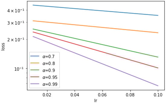
Figure 1. Effects of fractional order parameter $\alpha$, where $\mathrm{lr}=\eta$ denotes the learning rate.

Next, to make the effect of the neural network training experiment more clear and intuitive, the learning rate is fixed at 0.1 and 0.01. We compare the loss effects of the full batch gradient descent algorithm and the TFGD algorithm. The results are shown in Figure 2.

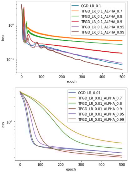
Figure 2. Comparison of loss effects for the learning rates $\eta =0.1,0.01$, and different fractional order parameter $\alpha$, where QGD and TFGD stand for the general gradient descent and the time-fractional gradient descent, respectively.

From Figure 2, we can verify the following two facts:

• For different learning rates ($\eta =0.01,0.1$) and the fractional order parameter $\alpha =0.99$, the effect of the neural network optimization based on the TFGD algorithm is significantly better than that of the general CD algorithm. Again, the fractional order parameter $\alpha$ is larger, and the optimization effect of the neural network is better.
• When $\eta =0.1,\alpha =0.99$ or $\eta =0.01,\alpha =0.9,0.99$, the loss effect of the TFGD algorithm is better than that of the general GD algorithm. However, the loss effect of TFGD is the same as that of the general GD if $\eta =0.01,\alpha =0.95$.

In a word, under the condition of selecting the appropriate learning rate, if the value of $\alpha$ is larger, the loss effect of the TFGD is better. This verifies that the memory dependence has an impact on the training of neural networks.

3.2. Empirical Analysis

To further determine the optimization effect of the TFGD algorithm in the neural network and to verify the accuracy of the previous numerical experiments, I apply the TFDG algorithm to the neural network optimization of real data. In the empirical analysis, I mainly use the classical handwritten digital data set, i.e., the MINST data set. To improve the efficiency of the training, the parameter $\alpha$ is taken as $[0.95,0.99]$, and the different learning rates $\eta =0.01,0.1$ are also selected.

The input data of this experimental model are 784-dimensional (28 × 28), the output data are one-dimensional, and the cross entropy is used as the loss function. To improve the efficiency of neural network training, the first 1000 data of handwritten digital data sets are selected for the experiment. We run the TFGD algorithm with 100 iterations. Under different learning rates ($\eta =0.01$ or $\eta =0.1$), the optimization effect of the TFGD algorithm is better than that of the general GD algorithm. Again, for the TFGD algorithm, the loss effect with $\alpha =0.99$ is better than that with $\alpha =0.95$. The corresponding results are shown in Figure 3.

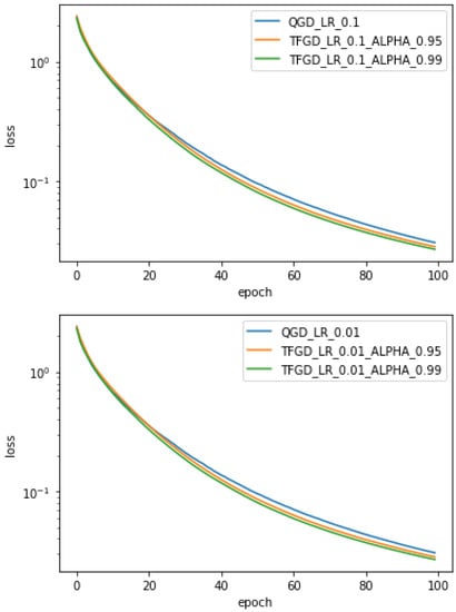
Figure 3. Comparison of loss effects for the learning rates $\eta =0.1$ and $\eta =0.01$, and the fractional order parameters $\alpha =0.95,0.99$, where QGD and TFGD stand for the general gradient descent and the time-fractional gradient descent, respectively.

In the above, armed with the classical handwritten digital data sets, the neural network training experiments based on the TFGD algorithm and the general GD algorithm are carried out, respectively. At different learning rates, we verify that the memory dependence affects neural network training.

4. Conclusions

This paper mainly studies the TFGD algorithm based on a weighted average to optimize the neural network training, which finally leads to the better generalization performance and the lower loss. Specifically, the parameter averaging method in neural network training can be regarded as memory-dependent, which just corresponds to an important feature of the time-fractional derivative. For theoretical analysis, the parameter averaging method is not convenient; however, the time-fractional derivative is more suitable. Again, the energy dissipation law and numerical stability of the time-fractional derivative are all inherited. Based on the above advantages, the new TFGD algorithm is proposed. We verify that the TFGD algorithm has potential advantages when the fractional order parameter $\alpha$ nears 0.95∼0.99. This implies that the memory dependence could improve the training performance of neural networks.

There are many exciting directions for future works. The TFGD algorithm is only applied to the function fitting and the image classification in one dimension. In order to verify the applicability and effectiveness of this algorithm, we consider more general numerical examples, such as fittings of the multi-dimensional function, CIFAR10, CIFAR100, and the other problems of image classification. The convergence analysis of this algorithm could be developed for future research. The TFGD algorithm is a new attempt that combines the averaging method in neural networks with the time-fractional gradient descent. We hope that the algorithm will inspire further work in this area.

References

- Bottou, L.; Curtis, F.; Nocedal, J. Optimization methods for large-scale machine learning. SIAM Rev. 2018, 60, 223–311. [Google Scholar] [CrossRef]
- Bottou, L. Large-scale machine learning with stochastic gradient descent. In Proceedings of the International Conference on Computational Statistics, Paris, France, 22–27 August 2010; pp. 177–186. [Google Scholar]
- Hardt, M.; Recht, B.; Singer, Y. Train faster, generalize better: Stability of stochastic gradient descent. In Proceedings of the International Conference on Machine Learning, New York, NY, USA, 19–24 June 2016. [Google Scholar]
- Polyak, B.T.; Juditsky, A.B. Acceleration of stochastic approximation by averaging. SIAM J. Control. Optim. 1992, 30, 838–855. [Google Scholar] [CrossRef]
- Zinkevich, M. Online convex programming and generalized infinitesimal gradient ascent. In Proceedings of the 20th International Conference on Machine Learning (ICML-03), Washington, DC, USA, 21–24 August 2003; pp. 928–936. [Google Scholar]
- Rakhlin, A.; Shamir, O.; Sridharan, K. Making gradient descent optimal for strongly convex stochastic optimization. arXiv 2011, arXiv:1109.5647. [Google Scholar]
- Shamir, O.; Zhang, T. Stochastic gradient descent for non-smooth optimization: Convergence results and optimal averaging schemes. In Proceedings of the International Conference on Machine Learning, Atlanta, GA, USA, 16–21 June 2013; pp. 71–79. [Google Scholar]
- Guo, Z.; Yan, Y.; Yang, T. Revisiting SGD with increasingly weighted averaging: Optimization and generalization perspectives. arXiv 2020, arXiv:2003.04339v3. [Google Scholar]
- Tao, W.; Pan, Z.; Wu, G.; Tao, Q. Primal averaging: A new gradient evaluation step to attain the optimal individual convergence. IEEE Trans. Cybern. 2020, 50, 835–845. [Google Scholar] [CrossRef] [PubMed]
- Izmailov, P.; Podoprikhin, D.; Garipov, T.; Vetrov, D.; Wilson, A.G. Averaging weights leads to wider optima and better generalization. In Proceedings of the 34th Conference on Uncertainty in Artificial Intelligence (UAI-2018), Monterey, CA, USA, 6–10 August 2018; pp. 876–885. [Google Scholar]
- Khan, S.; Malik, M.A.; Togneri, R.; Bennamoun, M. A fractional gradient descent-based RBF neural network. Circuits Syst. Signal Process. 2018, 37, 5311–5332. [Google Scholar] [CrossRef]
- Bao, C.; Pu, Y.; Zhang, Y. Fractional-order deep back propagation neural Network. Comput. Intell. Neurosci. 2018, 2018, 7361628. [Google Scholar] [CrossRef] [PubMed]
- Wang, J.; Wen, Y.; Gou, Y.; Ye, Z.; Chen, H. Fractional-order gradient descent learning of BP neural networks with Caputo derivative. Neural Netw. 2017, 89, 19–30. [Google Scholar] [CrossRef] [PubMed]
- Chen, M.; Chen, B.; Zeng, G.; Lu, K.; Chu, P. An adaptive fractional-order BP neural network based on extremal optimization for handwritten digits recognition. Neurocomputing 2020, 391, 260–272. [Google Scholar] [CrossRef]
- Wei, Y.; Kang, Y.; Yin, W.; Wang, Y. Generalization of the gradient method with fractional order gradient direction. J. Frankl. Inst. 2020, 357, 2514–2532. [Google Scholar] [CrossRef]
- Du, Q.; Yang, J.; Zhou, Z. Time-fractional Allen-Cahn equations: Analysis and numerical methods. J. Sci. Comput. 2020, 42, 85. [Google Scholar] [CrossRef]
- Liao, H.L.; Tang, T.; Zhou, T. An energy stable and maximum bound preserving scheme with variable time steps for time fractional Allen-Cahn equation. SIAM J. Sci. Comput. 2021, 43, A3503–A3526. [Google Scholar] [CrossRef]
- Liu, H.; Cheng, A.; Wang, H.; Zhao, J. Time-fractional Allen-Cahn and Cahn-Hilliard phase-field models and their numerical investigation. Comput. Math. Appl. 2018, 76, 1876–1892. [Google Scholar] [CrossRef]
- Quan, C.; Tang, T.; Yang, J. How to define dissipation-preserving energy for timefractional phase-field equations. CSIAM Trans. Appl. Math. 2020, 1, 478–490. [Google Scholar] [CrossRef]
- Tang, T.; Yu, H.; Zhou, T. On energy dissipation theory and numerical stability for time-fractional phase-field equations. SIAM J. Sci. Comput. 2019, 41, A3757–A3778. [Google Scholar] [CrossRef]
- Rahman, Z.; Abdeljabbar, A.; Roshid, H.; Ali, M.Z. Novel precise solitary wave solutions of two time fractional nonlinear evolution models via the MSE scheme. Fractal Fract. 2022, 6, 444. [Google Scholar] [CrossRef]
- Abdeljabbar, A.; Roshid, H.; Aldurayhim, A. Bright, dark, and rogue wave soliton solutions of the quadratic nonlinear Klein-Gordon equation. Symmetry 2022, 14, 1223. [Google Scholar] [CrossRef]
- Alsaedi, A.; Ahmad, B.; Kirane, M. Maximum principle for certain generalized time and space-fractional diffusion equations. Quart. App. Math. 2015, 73, 163–175. [Google Scholar] [CrossRef]
Publisher’s Note: MDPI stays neutral with regard to jurisdictional claims in published maps and institutional affiliations. |
© 2022 by the authors. Licensee MDPI, Basel, Switzerland. This article is an open access article distributed under the terms and conditions of the Creative Commons Attribution (CC BY) license (https://creativecommons.org/licenses/by/4.0/).