Complex Numbers Related to Semi-Antinorms, Ellipses or Matrix Homogeneous Functionals

Abstract

We generalize the property of complex numbers to be closely related to Euclidean circles by constructing new classes of complex numbers which in an analogous sense are closely related to semi-antinorm circles, ellipses, or functionals which are homogeneous with respect to certain diagonal matrix multiplication. We also extend Euler’s formula and discuss solutions of quadratic equations for the p-norm-antinorm realization of the abstract complex algebraic structure. In addition, we prove an advanced invariance property of certain probability densities.

1. Introduction

The history of complex numbers dates all the way back to the 16th century and begins with a period of ‘empirical’ discoveries and the derivation of surprising individual formulae, from which people observed the possibility of working successfully with imaginary numbers without being able to provide a satisfactory explanation. Later on, real masters expanded their usage of complex numbers in various computations, and some of them provided the first descriptions of these numbers. The continued search for a firm mathematical foundation, and with it a philosophical interpretation, lasted until the nineteenth century and can be followed in detail in [1], where the interested reader will find not only all the famous names involved until 1831, but also the remark that “in 1854 Richard Dedekind ...judged the situation differently”. Dedekind said at their Göttingen habilitation presentation in the presence of Gauss, ‘Until now, no theory of complex numbers has been accessible that is absolutely free from criticism ...or at least none has been published’.

The inexperienced reader may be referred to [2] for getting a first survey. Numerous standard introductions to mathematical analysis such as [3] or textbooks such as [4,5] discuss in detail all the usual rules for working with complex numbers. Therein, applications in physics and technique are considered, which represented corner stones in establishing complex numbers. Various fascinating verifications of the applicability of mathematical models to reality stimulated further theoretical and practical developments.

The classes of $l_p$-complex numbers which are generalizations of ordinary complex numbers are introduced for $p>0$ in [6] and are defined here for $p<0$. Closely following the approach in [6], both the classes of three-complex numbers and a general three-complex algebraic structure are introduced in [7].

Solving a quadratic equation within different realizations of an abstract complex algebraic structure allows the derivation of numerous new solutions beyond those known for the classical complex numbers. This will be shown in Section 2 of the present work for the $l_p$-realization. It turns out that the squaring of vectors representing complex numbers inside this realization may be shown rather nicely using pairings of $l_p$-circles ${\left|x\right|}^p+{\left|y\right|}^p=r_p^p$ of p-radius $r_p$. These circles are level sets of the corresponding $l_p$-norms or antinorms ${|(x,y)}^T{|}_p={\left(\right|x|}^p+{\left|y\right|}^p{)}^{1/p}$ if $p\ge 1$ or $p\in (0,1]$, respectively. Exactly the same analytical expression stands for a semi-antinorm if $p<0.$ This case is dealt with in Section 3 where semi-antinorm related complex numbers are introduced. The analytical definition of an elliptically vector multiplication and its geometric counterpart as well as the classes of elliptically complex numbers are introduced and some of their basic properties are considered in Section 4. This section might also serve as a short introduction to usual complex numbers just choosing the parameters $a=b=1$. The classes of complex numbers considered in Section 5 are closely related to $[p,q]$-circles $\frac{{\left|x\right|}^p}{p}+\frac{{\left|y\right|}^q}{q}=r$ with $p\ne q,$ which are the level sets of certain probability densities. The search for an advanced invariance property of such densities is presented in Section 6 and was one of author’s two motivations for doing the studies on generalized complex numbers in [6,7] and the present as well as another forthcoming one dealing with higher dimensions. The paper is finished by a concluding remark in Section 7.

For avoiding line breaks in some formulas and expressions such as ${\left({(x,y)}^T\right)}^k$ we use columns at some places.

A pair $(x,y)$ of real numbers representing a complex number is often written as $x+iy$ or, alternatively, as an element of the real vector space ${\mathbb{R}}^2.$

Before we begin, let us emphasize that the same ordered pair or vector ${(x,y)}^T$ representing a complex number may have different properties if it belongs to different spaces with different structures. This is because the axioms or rules of a space or algebraic structure determine the properties of its elements, not the other way around.

2. More Solutions to Quadratic Equations

The equation with respect to the variable z from the set of real numbers $\mathbb{R}$,

$$z^2+m·z+n=0,m\in \mathbb{R},n\in \mathbb{R}$$

(1)

has the solutions $z_{1/2}=-\frac{m}{2}\stackrel{+}{-}\sqrt{\frac{m^2}{4}-n}$ if the radicand is non-negative. Let us otherwise be given an abstract complex algebraic structure $(\mathbb{C},\oplus ,\odot ,·,\mathfrak{o},\mathfrak{e},\mathfrak{i})$ where $\mathbb{C}$ is a real vector space with operations of addition and scalar multiplication ⊕ and ·, respectively, ⊙ is an additional binary operation from $\mathbb{C}\times \mathbb{C}$ to $\mathbb{C}$, $(\mathbb{C},\oplus )$ and $(\mathbb{C},\odot )$ are Abelian groups with neutral elements $\mathfrak{0}$ and $\mathfrak{e}$, respectively, an element $\mathfrak{i}$ from $\mathbb{C}$ solves the equation $\mathfrak{i}\odot \mathfrak{i}=-\mathfrak{e}$, and distributivity of operations ⊕ and ⊙ holds. Then, the equation with respect to the variable z from $\mathbb{C}$,

$$z\odot z\oplus m·z\oplus n·\mathfrak{e}=\mathfrak{o}$$

(2)

can be reformulated as $z\odot z\oplus m·z\oplus \frac{m^2}{4}·\mathfrak{e}=(\frac{m^2}{4}-n)·\mathfrak{e}$ or $(z\oplus \frac{m}{2}·\mathfrak{e})\odot (z\oplus \frac{m}{2}·\mathfrak{e})=(n-\frac{m^2}{4})·\mathfrak{i}\odot \mathfrak{i}$ and its solutions are

$$z_{1/2}=-\frac{m}{2}·\mathfrak{e}\underset{\ominus }{\oplus }\sqrt{n-\frac{m^2}{4}}·\mathfrak{i}$$

(3)

with ⊖ denoting the naturally defined subtraction. Thus, the general structure of the solutions to Equation (2) does not depend on the concrete choice of the vector product rule ⊙.

In the usual notation of complex numbers in which $\mathfrak{i}=\sqrt{-1}$ is the ‘imaginary unit’, this means

$$z_{1/2}=-\frac{m}{2}\underset{-}{+}\sqrt{n-\frac{m^2}{4}}\sqrt{-1}$$

(4)

where, however, the operations + and − which combine the real number $-m/2$ with the undefined quantity $\sqrt{n-m^2/4}\sqrt{-1}$ are not intuitive for the novice reader, regardless matter how well he may already be using them.

Example 1.

Let $(\mathbb{C},\oplus ,\odot ,·,\mathfrak{e},\mathfrak{o},i)$ be the standard vector realization of the complex algebraic structure where $\mathbb{C}={\mathbb{R}}^2,\mathfrak{o}={(0,0)}^T,\mathfrak{e}={(1,0)}^T,i={(0,1)}^T$, ⊕ is the usual vector addition and the standard vector multiplication is defined by

$$\left(\begin{array}{c}{x}_1\\ y_1\end{array}\right)\odot \left(\begin{array}{c}{x}_2\\ y_2\end{array}\right)=\left(\begin{array}{c}{x}_1{x}_2-y_1{y}_2\\ y_1{x}_2+x_1{y}_2\end{array}\right)$$

meaning in the usual complex number writing that

$$(x_1+y_1\sqrt{-1})·(x_2+y_2\sqrt{-1})=x_1{x}_2-y_1{y}_2+(y_1{x}_2+x_1{y}_2)\sqrt{-1}.$$

This multiplication means in the special case of two identical vectors

$$\left(\begin{array}{c}x\\ y\end{array}\right)\odot \left(\begin{array}{c}x\\ y\end{array}\right)=\left(\begin{array}{c}{x}^2-y^2\\ 2xy\end{array}\right).$$

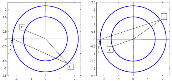
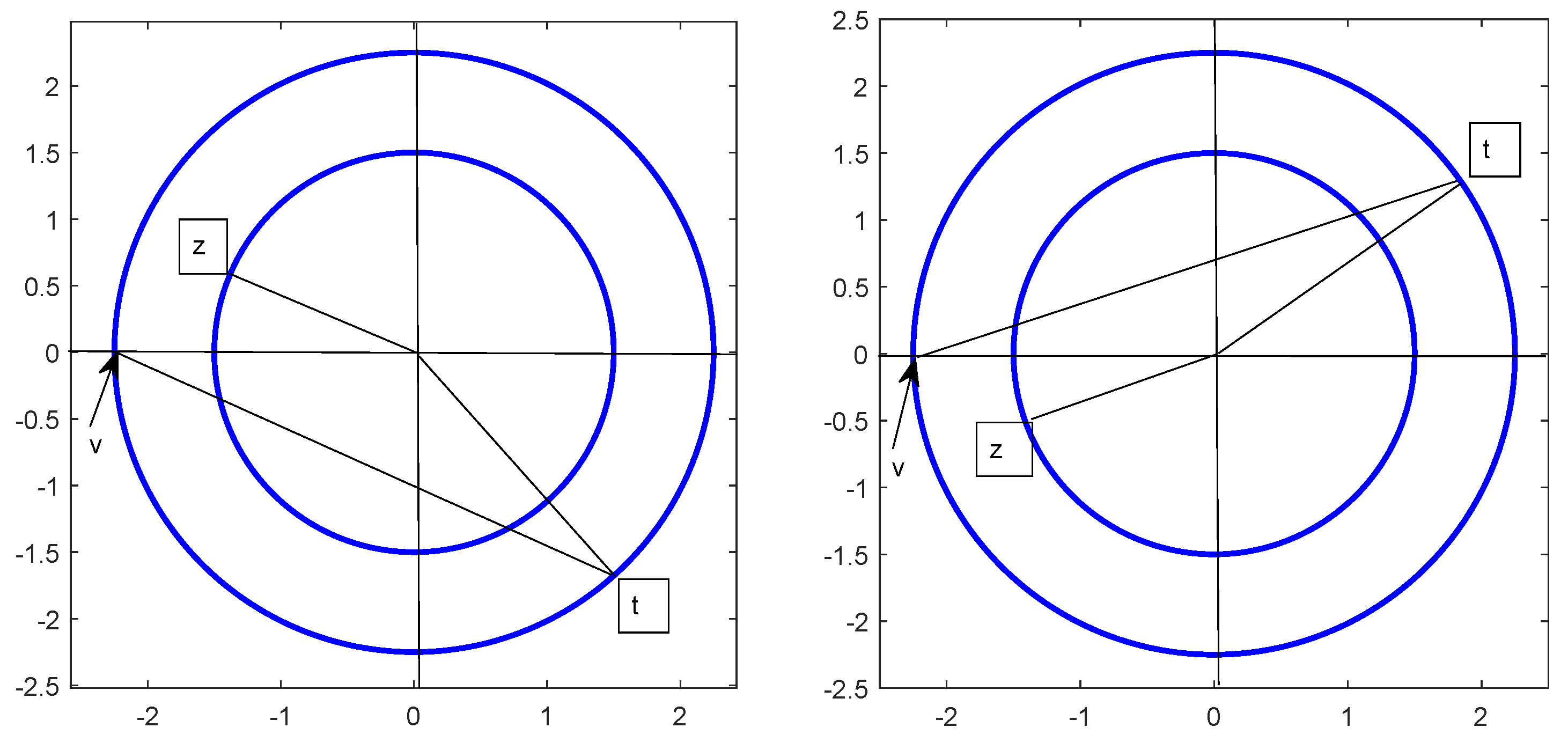
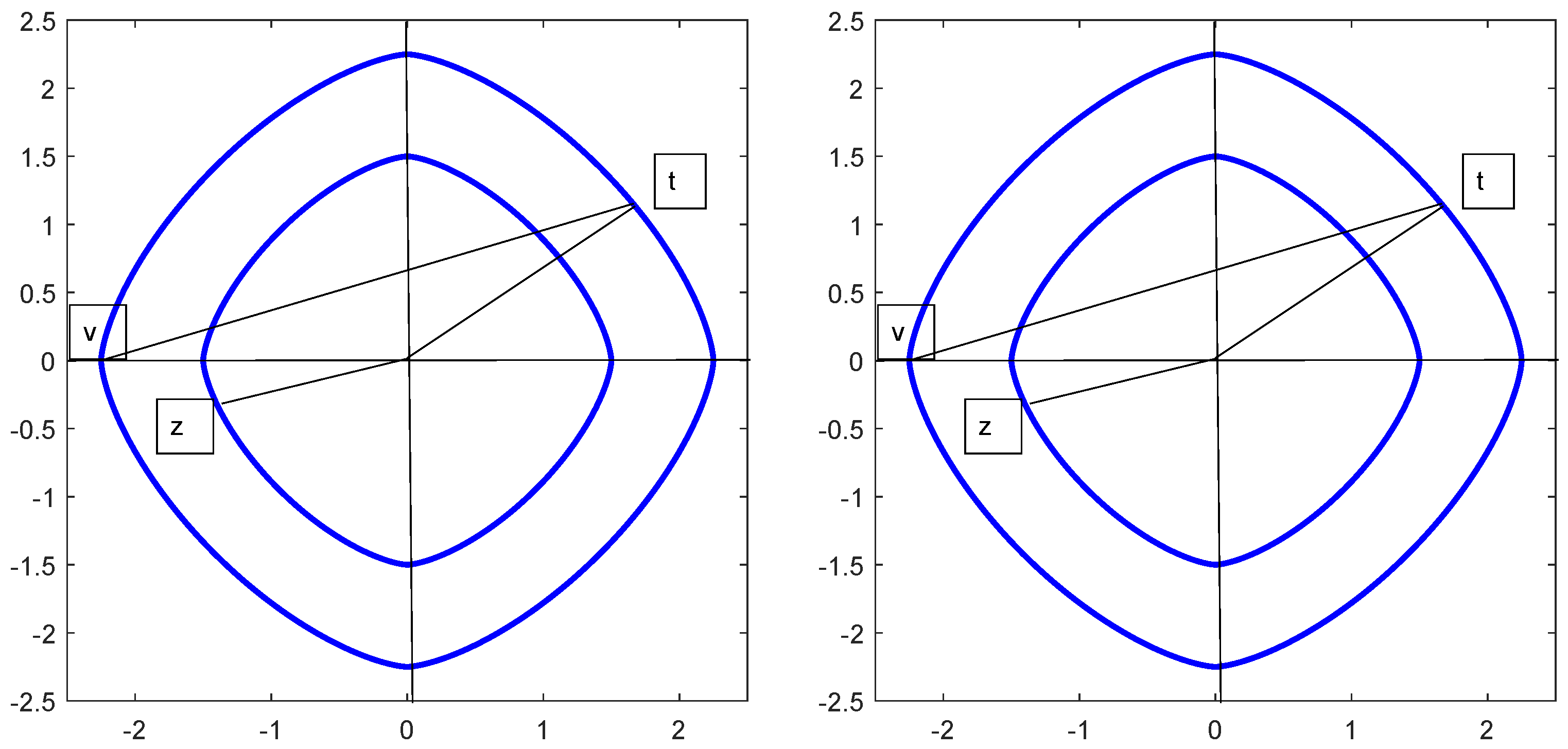
Let $z=\left(\begin{array}{c}-m/2\\ \underset{-}{+}\sqrt{n-m^2/4}\end{array}\right)=-\frac{m}{2}\stackrel{+}{-}\sqrt{n-m^2/4}\mathfrak{i}$ denote the solutions of Equation (2). Figure 1 shows an exemplary graphic illustration of where the vectors $z,t=z\odot z$ and $v=t+mz=-n\mathfrak{e}$ may be located in the space ${\mathbb{R}}^2$.

Figure 1. Geometry of quadratic equations with respect to standard vector multiplication. The Euclidean circles have the radii $\sqrt{n}=1.5$ and $n=2.25$, respectively.

Example 2.

Let us consider now the p-norm-antinorm realization $(\mathbb{C},\oplus ,{\odot }_p,·,\mathfrak{o},\mathfrak{e},i_p)$ of the abstract complex algebraic structure where $\mathbb{C},\mathfrak{o},\mathfrak{e},\oplus$ are as in Example 1, $i_p={(0,1)}^T$. Except if ${(x_l,y_l)}^T=\mathfrak{o}$ for at least one index $l\in \{1,2\}$, the vector p-multiplication $\odot ={\odot }_p$ is defined for every real $p>0$ according to [6] by

$$\left(\begin{array}{c}{x}_1\\ y_1\end{array}\right){\odot }_p\left(\begin{array}{c}{x}_2\\ y_2\end{array}\right)={\left[\frac{\left(\right|x_1{|}^p+|y_1{|}^p\left)\right(|x_2{|}^p+|y_2{|}^p)}{|x_1{x}_2-y_1{y}_2{|}^p+{|x_1{y}_2+y_1{x}_2|}^p}\right]}^{1/p}\left(\begin{array}{c}{x}_1\\ y_1\end{array}\right)\odot \left(\begin{array}{c}{x}_2\\ y_2\end{array}\right).$$

(5)

Moreover, we put $\mathfrak{o}{\odot }_p{(x,y)}^T=\mathfrak{o}$. This means in the special case of two identical vectors ${(x,y)}^T\ne \mathfrak{0},$

$$\left(\begin{array}{c}x\\ y\end{array}\right){\odot }_p\left(\begin{array}{c}x\\ y\end{array}\right)=\frac{{\left(\right|x|}^p+{\left|y\right|}^p{)}^{2/p}}{\left(\right|x^2-y^2{|}^p+2^p{\left|xy\right|}^p{)}^{1/p}}\left(\begin{array}{c}{x}^2-y^2\\ 2xy\end{array}\right).$$

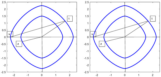
Let now $z=\left(\begin{array}{c}-m/2\\ \underset{-}{+}\sqrt{n-m^2/4}\end{array}\right)=-\frac{m}{2}\stackrel{+}{-}\sqrt{n-m^2/4}{i}_p$ denote the solutions of Equation (2). For an exemplary number $p\in (1,2)$, Figure 2 shows a graphic illustration of where the vectors $z,t=z{\odot }_{p}z$ and $v=t+mz=-n\mathfrak{e}$ are located in the space ${\mathbb{R}}^2$. As p changes, the shape of the p-circles also changes. We note that the element $\mathfrak{i}$ from $\mathbb{C}$ which appears in Equation (3) takes on the meaning of ${\mathfrak{i}}_p$ introduced in [6], and recall the last remark at the end of the Introduction. A geometrical view of Equation (5) which is given in [6] makes the associative nature of multiplication ${\odot }_p$ immediately visible.

Figure 2. Geometry of quadratic equations with respect to $l_p$-vector multiplication. The exemplary drawn p-circles (with $1<p<2$) have radii of the sizes $\sqrt{n}=1.5$ and $n=2.25$, similar figures can be drawn for $p\in (0,1]$ and $p>2$.

Example 3.

In the case of the so-called matrix realization of the abstract complex algebraic structure, $\mathbb{C}$ is the vector space of $2\times 2$-matrices of the type $x=\left(\begin{array}{cc}a& -b\\ b& a\end{array}\right),a\in \mathbb{R},b\in \mathbb{R}$ endowed with common matrix addition and multiplication ⊕ and ⊙, respectively, $\mathfrak{e}=\left(\begin{array}{cc}1& 0\\ 0& 1\end{array}\right),\mathfrak{o}=\left(\begin{array}{cc}0& 0\\ 0& 0\end{array}\right)$ and $\mathfrak{i}=\left(\begin{array}{cc}0& -1\\ 1& 0\end{array}\right).$

Example 4.

If $\mathbb{C}$ is the vector space of linear functions $f:\mathbb{R}\to \mathbb{R}$ defined for real a and b by $f\left(x\right)=ax+b,x\in \mathbb{R}$ then the sum of f and g where $g\left(x\right)=cx+d,x\in \mathbb{R}$ is defined by $(f+g)\left(x\right)=(a+c)x+b+d$, $\mathfrak{e}\left(x\right)=1,\mathfrak{o}\left(x\right)=0,\mathfrak{i}\left(x\right)=x\mathrm{and}(f\odot g)\left(x\right)=(ac-bd)x+ad+bc$. This way, another realization of $(\mathbb{C},\oplus ,\odot ,·,\mathfrak{0},\mathfrak{e},\mathfrak{i})$ is obtained which we call a linear function realization, and many more examples are possible.

The results of this section might encourage one to look at solutions of quadratic equations from a broadly applied point of view. The question to be answered in the case $n>m^2/4$ is whether embedding the solution of a given quadratic Equation (1) in the space $({\mathbb{R}}^2,|.{|}_2)$ is always the natural one, or whether embedding it in one of the spaces $({\mathbb{R}}^2,|.{|}_p)$ with $p\ne 2$ is even an option. For example, it might seem very unprofessional to an electric engineer to ask whether the current I and voltage U in an alternating current circuit definitely satisfy the equation $I^2\left(t\right)+U^2\left(t\right)=1$ in time or whether the equation ${\left|I\left(t\right)\right|}^p+{\left|U\left(t\right)\right|}^p=1$ for any $p\ne 2$ could also be an option; for a possible realization see (7) below. From a mathematical point of view, however, this may be considered the usual question of a suitable experiment to (as highly significant as possible) test the statistical null hypothesis $H_0:p=2$ versus the alternative hypothesis $H_A:p\ne 2,$ based on a suitable data set.

3. Semi-Antinorm Related Complex Numbers

The function ${|.|}_p:{\mathbb{R}}^2\to (0,\infty )$ defined by

$${\left|z\right|}_p={\left(\right|x|}^p+{\left|y\right|}^p{)}^{1/p},z={(x,y)}^T\in {\mathbb{R}}^2$$

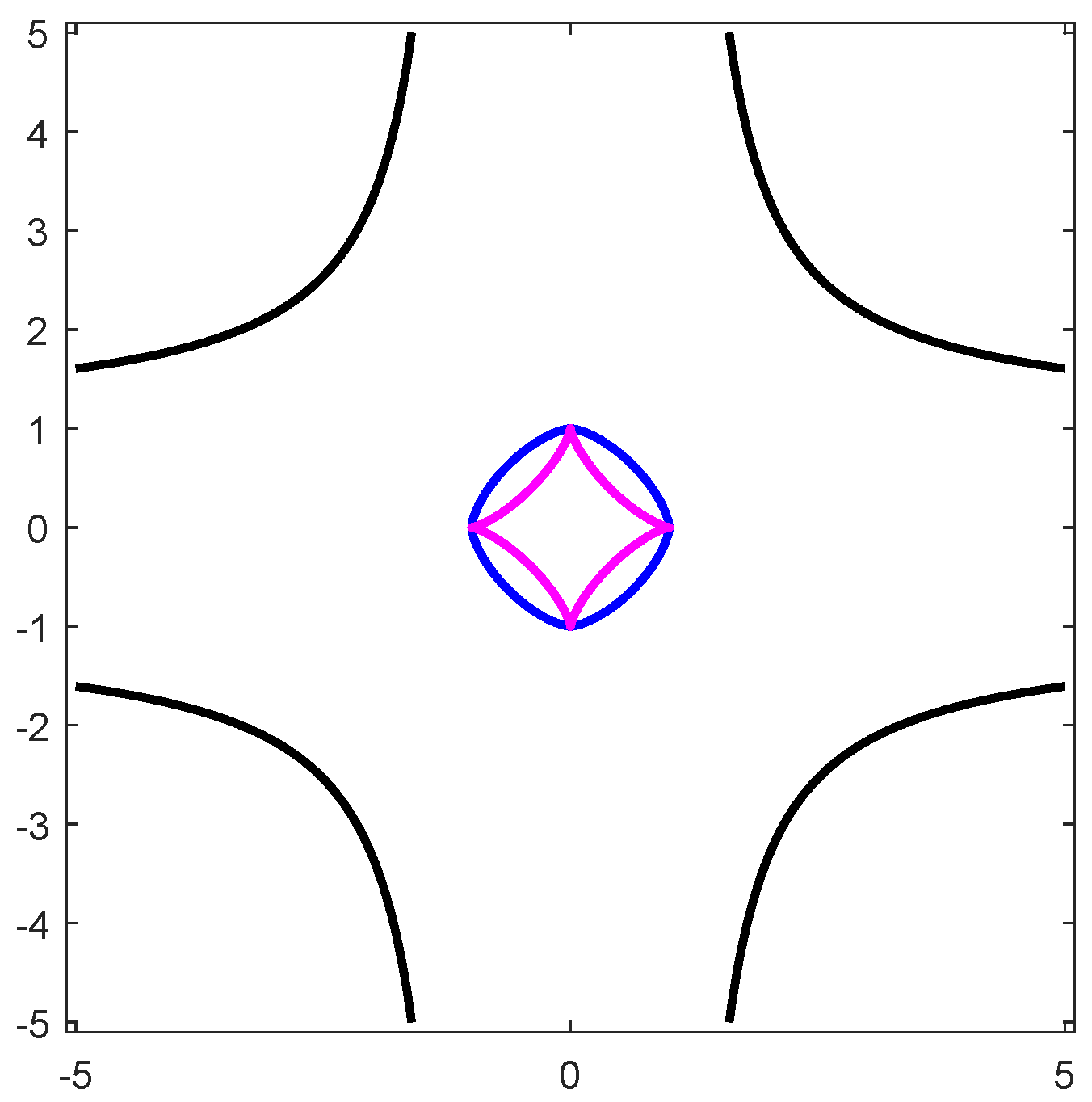
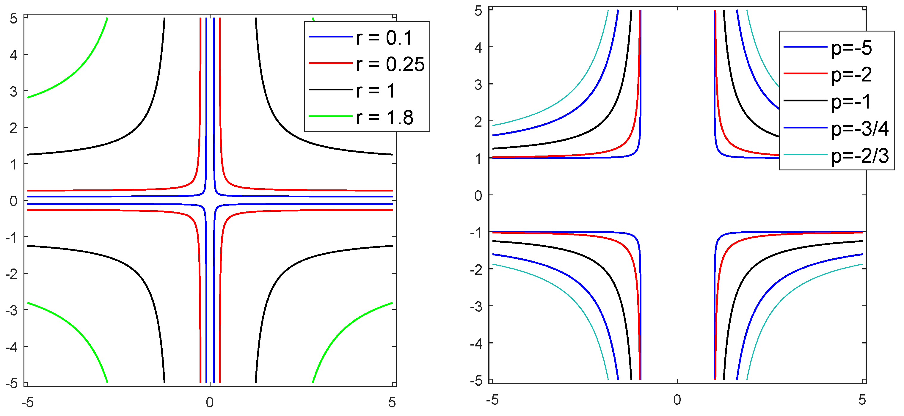
is a norm if $p\ge 1,$ an antinorm if $0<p\le 1$ and a semi-antinorm if $p<0,$ see Figure 3 and Figure 4. In the case of a semi-antinorm, the domain of definition is restricted by the assumption

$$x\ne 0\mathrm{and}y\ne 0.$$

(6)

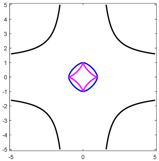
Figure 3. Level one lines of norm (blue), antinorm (pink) and semi-antinorm (black) ${\left|z\right|}_p$.

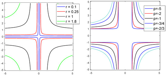
Figure 4. Level r lines of the semi-antinorm $z\to {\left|z\right|}_{-1}$ and level one lines of the semi-antinorms ${\left|z\right|}_p$ .

In [6], so-called $l_p$-complex numbers are derived using the function ${|.|}_p$ for $p>0.$ It turns out that only small technical changes are needed for adjusting this derivation to the case $p<0.$ It is therefore sufficient to present the main steps of this derivation, here. Due to the equivalence of the geometrical and the analytical approach we use the opportunity for a slight reorganization of the material compared to [6]. Throughout this section, we assume that $p<0$ and assumption (6) is satisfied.

Definition 1.

The vector p-product of $z_1={(x_1,y_1)}^T$ and $z_2={(x_2,y_2)}^T$ is defined by Equation (5), the k${}^{\prime }$th p-power of vector $z={(x,y)}^T$ and the p-exponential of z are defined by

$$z^k=z^{k-1}{\odot }_{p}z,k\ge 2,z^1=z,z^0={(1,0)}^{T}andex{p}_{\left[p\right]}\left(z\right)=\sum _{k=o}^{\infty }\frac{z^k}{k!},$$

respectively.

In this definition it is used that the norm convergence of the p-exponential of z follows from the ratio test. We recall now that Euler’s formula may be written as

$$cosx{(1,0)}^T+sinx{(0,1)}^T=e^{\sqrt{-1}x}.$$

Definition 2.

The quantity $e^{i_{p}x}$ is defined as the central projection of the point $cosx{(1,0)}^T+sinx{(0,1)}^T$ into the p-unit circle $C_p{\left(1\right)=\{(x,y)}^T{:|(x,y)}^T{|}_p=1\}$.

It follows that the p-generalized Euler formula

$$e^{i_{p}x}={cos}_p\left(x\right){(1,0)}^T\oplus {sin}_p\left(x\right){(0,1)}^T$$

is true where the p-generalized sine and cosine functions are defined by

$${sin}_p\left(\phi \right)=\frac{sin\phi }{N_p\left(\phi \right)}\mathrm{and}{cos}_p\left(\phi \right)=\frac{cos\phi }{N_p\left(\phi \right)}$$

with

$$N_p\left(\phi \right)={\left(\right|sin\phi |}^p+{|cos\phi |}^p{)}^{1/p},\phi \in {(0,2\pi )}^{*}=(0,2\pi )\backslash \{\frac{\pi }{2},\pi ,\frac{3\pi }{2}\}.$$

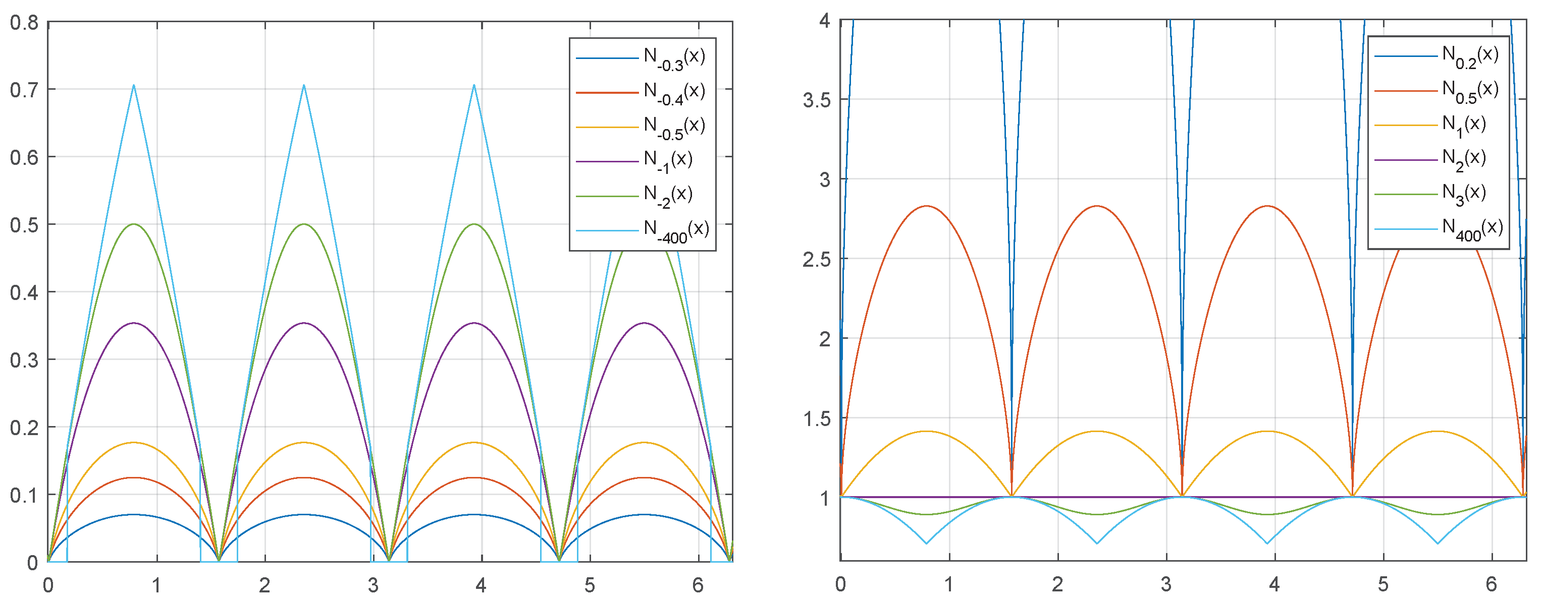
A graphical illustration of these functions is given in Figure 5 and Figure 6. Obviously, these trigonometric functions satisfy the equation

$$|{sin}_p{\left(\phi \right)|}^p+{\left|{cos}_p\left(\phi \right)\right|}^p=1.$$

(7)

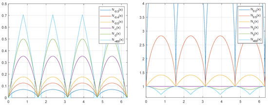
Figure 5. The function $N_p$ for several values of $p.$

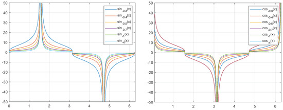
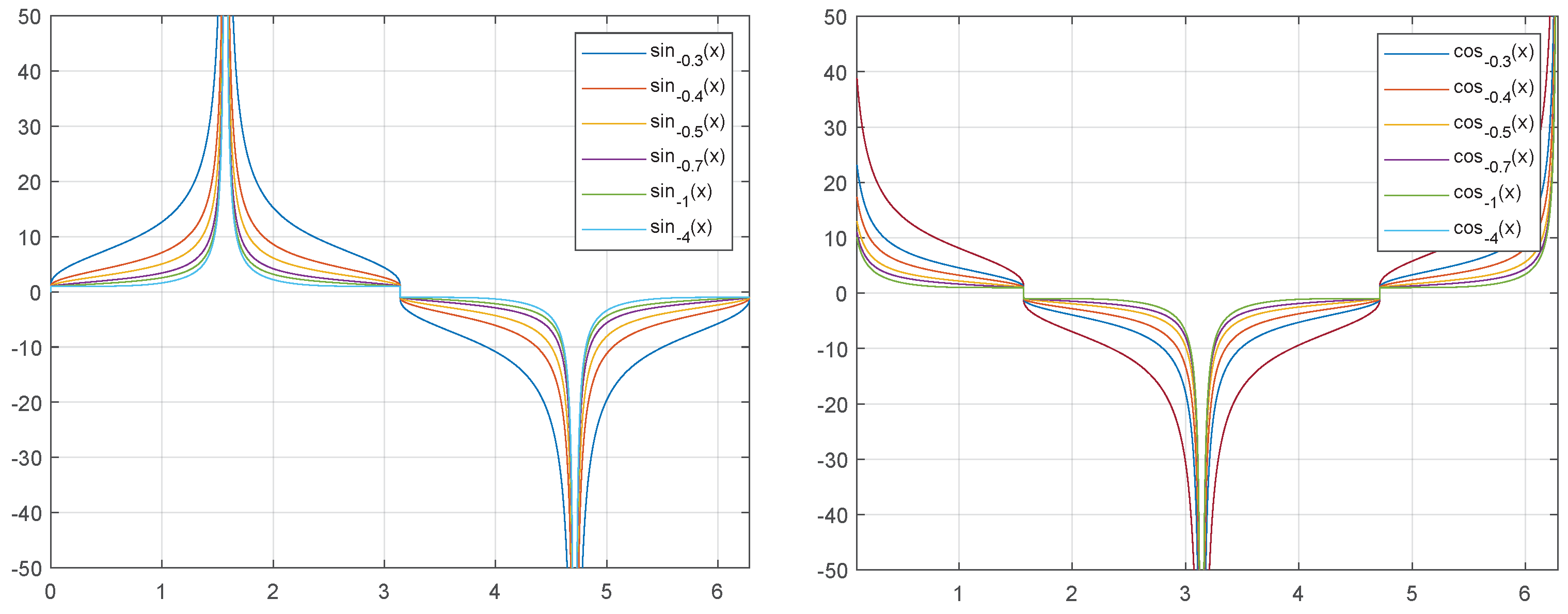
Figure 6. The p-generalized sine and cosine functions, $p<0$. For figures in case $p>0$, see [7]. The jumps that are seen in multiples of $\pi /2$ occur from +1 to −1, or vice versa.

Definition 3.

The p-complex exponential function $ex{p}_{\left(p\right)}:\mathbb{R}\to {\mathbb{R}}^2$ is defined as

$$ex{p}_{\left(p\right)}\left(x\right)=ex{p}_{\left[p\right]}\left(x\left(\begin{array}{c}1\\ 0\end{array}\right)\right).$$

It follows from the p-generalized Euler formula that

$$e^{i_{p}x}=N_p^{-1}\left(x\right)ex{p}_{\left(p\right)}\left(x\right).$$

In the rest of this section, the analytical definition of the vector p-product for $p<0$, in Definition 1, will by expressed equivalently in a geometric way. For this purpose, we define the $l_p$-type polar coordinate transformation $Po{l}_p:(0,\infty )\times {(0,2\pi )}^{*}\to {\mathbb{R}}^2$ for the present case $p<0$ as ${(x,y)}^T=Po{l}_p[r,\phi ]$ with

$$x=r{cos}_p\left(\phi \right),y=r{sin}_p\left(\phi \right).$$

This transformation is almost everywhere invertible,

$$r={\left(\right|x|}^p+{\left|y\right|}^p{)}^{1/p}\mathrm{and}\phi =arctan\frac{y}{x}.$$

The semi-antinorm level r sets, or semi-antinorm circles of p-radius r,

$$C_p{\left(r\right)=\{z=(x,y)}^T{:\left|z\right|}_p=r\},r>0$$

are pairwise disjoint and their union is almost surely equal to ${\mathbb{R}}^2$, see Figure 4. The proof of the following theorem follows [6] and is therefore be omitted here.

Theorem 1.

The vector p-product of $z_1=Po{l}_p[r_1,{\phi }_1]$ and $z_2=Po{l}_p[r_2,{\phi }_2]$ can be expressed geometrically equivalently as $z_1{\odot }_p{z}_2=Po{l}_p[r_1{r}_2,{\phi }_1+{\phi }_2]$ where the angle ${\phi }_1+{\phi }_2$ is defined modulo 2π.

The vector p-product is graphically illustrated in Figure 7.

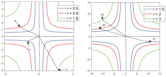
Figure 7. Vector p-products $w=u{\odot }_{-1}v$ and $z=z1{\odot }_{-2/3}z2$.

Remark 1.

(a) 

Because of the assumption (6), those φ-angles that appear in this theorem do not attain values that are multiples of $\pi /2$.

(b) 

In conclusion, let us name the invariance property that the semi-antinorm ${|.|}_p$-value of a vector in ${\mathbb{R}}^2$ is not changed when multiplied by a vector which has semi-antinorm ${|.|}_p$-value one. In other words, for every $r>0,$ the Lie group on $C_p\left(r\right)$ consists of all transformations ${(x,y)}^T\to {(x,y)}^T{\odot }_{p}z$ where z is an arbitrary element of $C_p\left(1\right).$

(c) 

The particular vector p-multiplication of a vector $z\in {\mathbb{R}}^2$ by $\mathfrak{e}={(1,0)}^T$ results in vector z.

Definition 4.

For every $p\in \mathbb{R},$ we call $({\mathbb{R}}^2,\oplus ,{\odot }_p,·,\mathfrak{o},\mathfrak{e},i_p)$ a p-complex plane. In particular, such plane is called a norm related complex plane if $p\ge 1,$ an antinorm related complex plane if $0<p\le 1$ and a semi-antinorm related complex plane if $p<0.$

Consideration of the limiting situation $p\to 0$ as well as cases of more general functionals is left open, here.

4. Elliptical Complex Numbers

The studies in [6,7] and so far in the present paper suggest that there is always a vector analytical, a complex analytical and a geometric component of the material when introducing a new kind of generalized complex numbers. These components define the structure of this section.

4.1. Vector Analysis

Let $a>0,b>0$ and ${\left|z\right|}_{(a,b)}={\left({\left(\frac{x}{a}\right)}^2+{\left(\frac{y}{b}\right)}^2\right)}^{1/2}$ the $(a,b)$-norm of $z={(x,y)}^T\in {\mathbb{R}}^2.$

Definition 5.

If at least one of the vectors $z_i={(x_i,y_i)}^T\in {\mathbb{R}}^2,i=1,2$ is equal to $\mathfrak{o}={(0,0)}^T$ then we define the elliptical vector $(a,b)$-product to be $\mathfrak{o}$, otherwise

$$z_1{\odot }_{(a,b)}{z}_2=|z_1{|}_{(a,b)}{\left|z_2\right|}_{(a,b)}\frac{z_1\odot z_2}{|z_1\odot z_2{|}_{(a,b)}}.$$

(8)

This vector-product is commutative and associative and means in the particular case of two identical vectors

$$\left(\begin{array}{c}x\\ y\end{array}\right){\odot }_{(a,b)}\left(\begin{array}{c}x\\ y\end{array}\right)=\frac{{\left(\frac{x}{a}\right)}^2+{\left(\frac{y}{b}\right)}^2}{{\left({\left(\frac{x^2-y^2}{a}\right)}^2+{\left(\frac{2xy}{b}\right)}^2\right)}^{1/2}}\left(\begin{array}{c}{x}^2-y^2\\ 2xy\end{array}\right).$$

Moreover, $z\odot z=(-z)\odot (-z)$ while ${\left(w\right)}^2\ne {(-w)}^2$ for a basis number in [8].

The structure of the product in Equation (8) is obviously very similar to that in Equation (5) and the particular product $z_1{\odot }_{(1,1)}{z}_2=z_1\odot z_2$ is just the usual complex number multiplication. The elliptical vector $(a,b)$-multiplication satisfies

$$|z_1{\odot }_{(a,b)}{z}_2{|}_{(a,b)}=|z_1{|}_{(a,b)}·{\left|z_2\right|}_{(a,b)}$$

(9)

and

$$\left(A_1{z}_1\right){\odot }_{(a,b)}\left(A_2{z}_2\right)=\left(A_1{A}_2\right)\left(z_1{\odot }_{(a,b)}{z}_2\right),A_i\in \mathbb{R},i=1,2.$$

(10)

Equation (9) means that the squares of the $(a,b)$-elliptical radii of $z_1,z_2$ and the product $z=z_1{\odot }_{(a,b)}{z}_2$ satisfy the equation $r^2=r_1^2{r}_2^2,$ that is

$${\left(\frac{x}{a}\right)}^2+{\left(\frac{y}{b}\right)}^2=\left({\left(\frac{x_1}{a}\right)}^2+{\left(\frac{y_1}{b}\right)}^2\right)\left({\left(\frac{x_2}{a}\right)}^2+{\left(\frac{y_2}{b}\right)}^2\right).$$

(11)

The $(a,b)$-multiplicative neutral element is ${(a,0)}^T$ and the $(a,b)$-multiplicative inverse element of $z={(x,y)}^T\ne \mathfrak{o}$ is

$$z_{(a,b)}^{-1}=\frac{1}{{\left|z\right|}_{(a,b)}^2}\left(\begin{array}{c}x\\ -y\end{array}\right).$$

Definition 6.

We define the elliptical vector $(a,b)$-division of $z_1\in {\mathbb{R}}^2$ by $z_2\in {\mathbb{R}}^2,z_2\ne \mathfrak{o}$ by

$$z_1{\oslash }_{(a,b)}{z}_2=z_1{\odot }_{(a,b)}{\left(z_2\right)}_{(a,b)}^{-1}.$$

This vector-division can be represented more explicitly as

$$z_1{\oslash }_{(a,b)}{z}_2=\frac{|z_1{|}_{(a,b)}}{|z_2{|}_{(a,b)}}\frac{z_1\oslash z_2}{|z_1\oslash z_2{|}_{(a,b)}}\mathrm{with}{z}_1{\oslash }_{(a,b)}{z}_2=\left(\begin{array}{c}{x}_1{x}_2+y_1{y}_2\\ y_1{x}_2-x_1{y}_2\end{array}\right).$$

(12)

For $z\in {\mathbb{R}}^2$, we put $z^{\left(0\right|a,b)}=\left(\begin{array}{c}a\\ 0\end{array}\right)$ and define the k’th elliptical vector power (or k’th vector $(a,b)$-power) by $z^{\left(k\right|a,b)}=z^{(k-1|a,b)}{\odot }_{(a,b)}z,k=1,2,\dots$

Example 5.

The elliptical vector $(a,b)$-multiplication and k’th elliptical vector power satisfy the following particular rules

$$\left(\begin{array}{c}0\\ 1\end{array}\right){\odot }_{(a,b)}\left(\begin{array}{c}0\\ 1\end{array}\right)=-\frac{a}{b^2}\left(\begin{array}{c}1\\ 0\end{array}\right),$$

(13)

$$\left(\begin{array}{c}1\\ 0\end{array}\right){\odot }_{(a,b)}\left(\begin{array}{c}0\\ 1\end{array}\right)=\frac{1}{a}\left(\begin{array}{c}0\\ 1\end{array}\right),$$

(14)

$${\left(\begin{array}{c}0\\ 1\end{array}\right)}^{\left(2k\right|a,b)}={(-1)}^k\frac{a}{b^{2k}}\left(\begin{array}{c}1\\ 0\end{array}\right)and{\left(\begin{array}{c}0\\ 1\end{array}\right)}^{(2k+1|a,b)}={(-1)}^k\frac{1}{b^{2k}}\left(\begin{array}{c}0\\ 1\end{array}\right),k=1,2,\dots .$$

(15)

We introduce now a new type of exponential function. The ratio test ensures norm convergence of the following sum.

Definition 7.

The elliptical $(a,b)$-exponential function $ex{p}_{(a,b)}:\mathbb{R}\to {\mathbb{R}}^2$ is defined by

$$ex{p}_{(a,b)}\left(x\right)=\sum _{k=0}^{\infty }\frac{x^k}{k!}{\left(\begin{array}{c}0\\ 1\end{array}\right)}^{\left(k\right|a,b)}.$$

Theorem 2.

The geometric $(a,b)$-exponential function allows the trigonometric representation

$$ex{p}_{(a,b)}\left(\frac{t}{a}\left(\begin{array}{c}0\\ 1\end{array}\right)\right)=acos\left(\frac{t}{ab}\right)\left(\begin{array}{c}1\\ 0\end{array}\right)+bsin\left(\frac{t}{ab}\right)\left(\begin{array}{c}0\\ 1\end{array}\right),t\in \mathbb{R}.$$

Proof. 

The norm convergent series expansion

$$ex{p}_{(a,b)}\left(\frac{t}{a}\left(\begin{array}{c}0\\ 1\end{array}\right)\right)={\left(\begin{array}{c}0\\ 1\end{array}\right)}^{\left(0\right)}+\frac{t}{a}{\left(\begin{array}{c}0\\ 1\end{array}\right)}^{\left(1\right)}+\frac{t^2}{2!a^2}{\left(\begin{array}{c}0\\ 1\end{array}\right)}^{\left(2\right)}+\frac{t^3}{3!a^3}{\left(\begin{array}{c}0\\ 1\end{array}\right)}^{\left(3\right)}+\dots$$

can be re-arranged as

$$ex{p}_{(a,b)}\left(\frac{t}{a}\left(\begin{array}{c}0\\ 1\end{array}\right)\right)=a\left[1-\frac{t^2}{2!{\left(ab\right)}^2}+\frac{t^4}{4!{\left(ab\right)}^4}-\frac{t^6}{6!{\left(ab\right)}^6}+\dots \right]\left(\begin{array}{c}1\\ 0\end{array}\right)$$

$$+b\left[\frac{t}{ab}-\frac{t^3}{3!{\left(ab\right)}^3}+\frac{t^5}{5!{\left(ab\right)}^5}-\frac{t^7}{7!{\left(ab\right)}^7}+\dots \right]\left(\begin{array}{c}0\\ 1\end{array}\right).$$

□

4.2. Complex Analysis

With ⊕ denoting usual vector addition, every vector $z={(x,y)}^T\in {\mathbb{R}}^2$ can be represented as

$$z=\frac{x}{a}\left(\begin{array}{c}a\\ 0\end{array}\right)\oplus \frac{y}{b}\left(\begin{array}{c}0\\ b\end{array}\right)=\frac{x}{a}\mathfrak{e}+\frac{y}{b}{i}_{(a,b)}$$

where $\mathfrak{e}={(a,0)}^T$ is the $(a,b)$-multiplicative neutral element and $i_{(a,b)}={(0,b)}^T$ is called the $(a,b)$-imaginary unit. Adopted to usual notion of complex numbers, this reads

$$z=\frac{x}{a}+\frac{y}{b}{i}_{(a,b)}.$$

Equation (13) may be rewritten as

$$i_{(a,b)}{\odot }_{(a,b)}{i}_{(a,b)}=-\mathfrak{e}$$

or $i_{(a,b)}^2=-1$, for short. Elliptical vector $(a,b)$-multiplication of $z_1$ by $z_2$ can be written in this sense as

$$\begin{array}{c}\hfill \left(\frac{x_1}{a}+\frac{y_1}{b}{i}_{(a,b)}\right){\odot }_{(a,b)}\left(\frac{x_2}{a}+\frac{y_2}{b}{i}_{(a,b)}\right)=\frac{{({\left(\frac{x_1}{a}\right)}^2+{\left(\frac{y_1}{b}\right)}^2)}^{1/2}{({\left(\frac{x_2}{a}\right)}^2+{\left(\frac{y_2}{b}\right)}^2)}^{1/2}}{{({\left(\frac{x_1{x}_2-y_1{y}_2}{a}\right)}^2+{\left(\frac{y_1{x}_2+x_1{y}_2}{b}\right)}^2)}^{1/2}}\\ \hfill \times [(x_1{x}_2-y_1{y}_2)+(y_1{x}_2+x_1{y}_2)i_{(a,b)}].\end{array}$$

In other words,

$$\begin{array}{c}\hfill ({\xi }_1+{\eta }_1{i}_{(a,b)}){\odot }_{(a,b)}({\xi }_2+{\eta }_2{i}_{(a,b)})=\frac{{({\xi }_1^2+{\eta }_1^2)}^{1/2}{({\xi }_2^2+{\eta }_2^2)}^{1/2}}{{({\left(a{\xi }_1{\xi }_2-\frac{b^2}{a}{\eta }_1{\eta }_2\right)}^2+{\left(a({\eta }_1{\xi }_2+{\xi }_1{\eta }_2)\right)}^2)}^{1/2}}\\ \hfill \times [(a^2{\xi }_1{\xi }_2-b^2{\eta }_1{\eta }_2)+ab({\eta }_1{\xi }_2+{\xi }_1{\eta }_2)i_{(a,b)}]\end{array}$$

(16)

where ${\xi }_l$ and ${\eta }_l$ are the coordinates of $z_l$ with respect to the basis $\{{(a,0)}^T,{(0,b)}^T\}$.

Theorem 2 reads alternatively as the following generalization of Euler’s formula

$${exp}_{(a,b)}\left(i_{(a,b)}\frac{t}{ab}\right)=cos\left(\frac{t}{ab}\right)+sin\left(\frac{t}{ab}\right)i_{(a,b)}.$$

(17)

Definition 8.

For every pair $(a,b)$ with $a>0,b>0,$ we call the complex algebraic structure ${\mathbb{C}}_{(a,b)}=({\mathbb{R}}^2,\oplus ,{\odot }_{(a,b)},·,\mathfrak{o},\mathfrak{e},i_{(a,b)})$ the $(a,b)$-elliptical complex plane.

Obviously, ${\mathbb{C}}_{(1,1)}$ is the usual complex plane.

Example 6.

Let $t=\pi (a,b)=ab\pi$ be the ellipse number, then

$${exp}_{(a,b)}\left(i_{(a,b)}\pi \right)+1=0.$$

4.3. Geometric View

It is easily seen that the elliptical vector $(a,b)$-multiplication by an $(a,b)$-unit vector leaves the $(a,b)$-norm of a given vector invariant, that is if $|z_2{|}_{(a,b)}=1$ then we have $|z_1{\odot }_{(a,b)}{z}_2{|}_{(a,b)}={\left|z_1\right|}_{(a,b)}$. Thus, the Lie group on an arbitrary ellipse

$$E_{(a,b)}\left(r\right)=\{z\in {\mathbb{R}}^2{:\left|z\right|}_{(a,b)}=r\},r>0$$

is the set of transformations $\left(\begin{array}{c}x\\ y\end{array}\right)\to \left(\begin{array}{c}x\\ y\end{array}\right){\odot }_{(a,b)}z$ with z satisfying ${\left|z\right|}_{(a,b)}=1$. This can also be described using suitable coordinates. To this end, let the $(a,b)$-elliptical polar coordinate transformation $Po{l}_{(a,b)}:[0,\infty )\times [0,2\pi )\to {\mathbb{R}}^2$ be defined by

$${(x,y)}^T=Po{l}_{(a,b)}[r,\phi ]={(ra{cos}_{(a,b)}\left(\phi \right),rb{sin}_{(a,b)}\left(\phi \right))}^T$$

where generalized trigonometric functions are defined as

$${cos}_{(a,b)}\left(\phi \right)=\frac{cos\phi }{a{N}_{(a,b)}\left(\phi \right)}\mathrm{and}{sin}_{(a,b)}\left(\phi \right)=\frac{sin\phi }{b{N}_{(a,b)}\left(\phi \right)}$$

with

$$N_{(a,b)}\left(\phi \right)={\left|(cos\phi ,sin\phi )\right|}_{(a,b)},$$

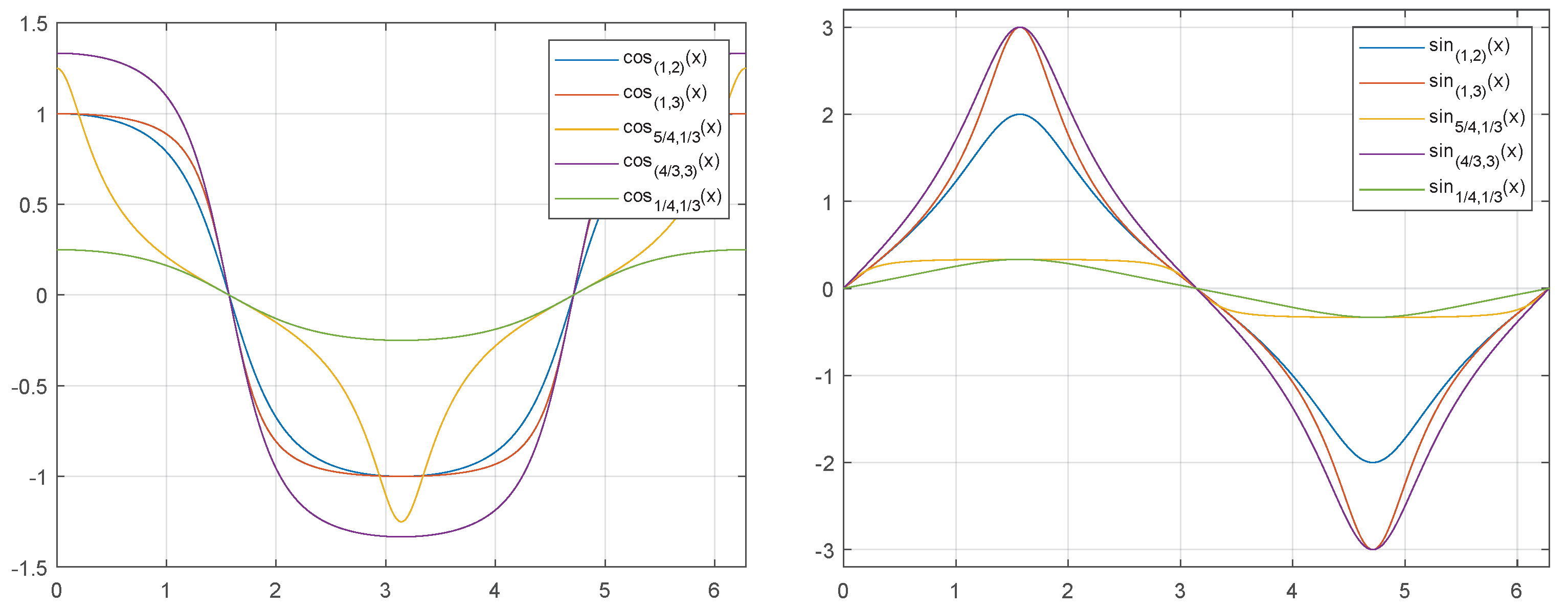
see Figure 8.

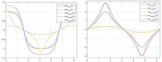
Figure 8. The elliptical trigonometric functions ${cos}_{(a,b)}$ and ${sin}_{(a,b)}$.

This transformation is a.e. invertible with

$${r=|(x,y)}^T{|}_{(a,b)}\mathrm{and}\phi =arctan\frac{y}{x}.$$

Theorem 3.

For any two elements from ${\mathbb{R}}^2,$$z_i=Po{l}_{(a,b)}[r_i,{\phi }_i],i=1,2$ the elliptical vector $(a,b)$-product can be represented as

$$z_1{\odot }_{(a,b)}{z}_2=Po{l}_{(a,b)}[r_1{r}_2,{\phi }_1+{\phi }_2]$$

(18)

where the angle ${\phi }_1+{\phi }_2$ is to be chosen modulo $2\pi$.

Proof. 

It follows from

$$|Po{l}_{(a,b)}[r_1{r}_2,{\phi }_1+{\phi }_2]{|}_{(a,b)}=|z_1{|}_{(a,b)}{\left|z_2\right|}_{(a,b)}$$

and, with $\left|z\right|={\left|z\right|}_{(1,1)}={\left|z\right|}_2,$

$$r_1{r}_2{(a{cos}_{(a,b)}({\phi }_1+{\phi }_2),b{sin}_{(a,b)}({\phi }_1+{\phi }_2))}^T=\frac{|z_1{|}_{(a,b)}{\left|z_2\right|}_{(a,b)}}{|z_1\left|\right|z_2|N_{(a,b)}({\phi }_1+{\phi }_2)}{z}_1\odot z_2$$

that

$$N_{(a,b)}({\phi }_1+{\phi }_2)=\frac{|z_1\odot z_2{|}_{(a,b)}}{|z_1\left|\right|z_2|},$$

thus

$$Po{l}_{(a,b)}[r_1{r}_2,{\phi }_1+{\phi }_2]=|z_1{|}_{(a,b)}{\left|z_2\right|}_{(a,b)}\frac{z_1\odot z_2}{|z_1\odot z_2{|}_{(a,b)}}.$$

□

For an analog geometric background of $l_p$-complex and three-complex numbers, see [6,7].

Remark 2.

Distributivity of vector addition and multiplication is missing in the complex algebraic structure $({\mathbb{R}}^2,\oplus ,{\odot }_{(a,b)},·,\mathfrak{0},\mathfrak{e},i_{(a,b)})$.

Remark 3.

If one considers scaling $z\to \tilde{z}={(\frac{x}{a},\frac{y}{b})}^T$ and usual complex vector multiplication ${\tilde{z}}_1\odot {\tilde{z}}_2={(\frac{x_1{x}_2}{a^2}-\frac{y_1{y}_2}{b^2},\frac{x_1{y}_2+y_1{x}_2}{ab})}^T$ then $|{\tilde{z}}_1\odot {\tilde{z}}_2{|}_2={\left|{\tilde{z}}_1\right|}_2$ for all ${\tilde{z}}_2$ satisfying $|{\tilde{z}}_2{|}_2=1$. This invariance property is closely related to that of orthogonal transformations in the complex plane letting the absolute value of complex numbers invariant. Nevertheless, the present approach to elliptical complex numbers cannot be traced back to ordinary complex numbers this way because ${\tilde{z}}_1\odot {\tilde{z}}_2$ is not equal to $z_1{\odot }_{(a,b)}{z}_2$ according to (8), in general, and does therefore not allow the geometric interpretation in (18).

5. Complex Numbers Related to Matrix Homogeneous Functionals

In the present section we start with a geometric consideration for introducing another vector multiplication and turn over only later to its analytical formulation and the corresponding complex analysis. To this end, let $p>0, q>0$ be real numbers and $Po{l}_{[p,q]}:(0,\infty )\times [0,2\pi )\to {\mathbb{R}}^2\backslash \left\{{(0,0)}^T\right\}$ the $[p,q]$-generalized or $[p,q]$-spherical polar coordinate transformation defined by

$$z={(x,y)}^T=Po{l}_{[p,q]}(r,\phi )={({\left(pr\right)}^{1/p}{cos}_{pq,q}\left(\phi \right),{\left(qr\right)}^{1/q}{sin}_{pq,p}\left(\phi \right))}^T$$

with

$${cos}_{\lambda ,\gamma }\left(\phi \right)=sign(cos\phi )|{cos}_{\lambda }{\left(\phi \right)|}^{\gamma },{sin}_{\lambda ,\gamma }\left(\phi \right)=sign(sin\phi ){\left|{sin}_{\lambda }\left(\phi \right)\right|}^{\gamma }$$

where

$${cos}_{\lambda }\left(\phi \right)=\frac{cos\phi }{N_{\lambda }\left(\phi \right)}\mathrm{and}{sin}_{\lambda }\left(\phi \right)=\frac{sin\phi }{N_{\lambda }\left(\phi \right)}$$

as well as

$$N_{\lambda }\left(\phi \right)={\left(\right|sin\phi |}^{\lambda }+{|cos\phi |}^{\lambda }{)}^{1/\lambda }.$$

The a.e. defined inverse coordinate transformation satisfies

$${r=|(x,y)}^T{|}_{[p,q]}\mathrm{and}\phi =arctan\left[sign\left(xy\right){\left(\frac{p}{q}\right)}^{1/\left(pq\right)}\frac{{\left|y\right|}^{1/p}}{{\left|x\right|}^{1/q}}\right]$$

where the functional

$${|(x,y)}^T{|}_{[p,q]}=\frac{{\left|x\right|}^p}{p}+\frac{{\left|y\right|}^q}{q}$$

is a norm if $p=q\ge 1$ and an antinorm if $p=q\in (0,1]$. It is reasonable therefore to assume that $p\ne q$ throughout this section.

The functional ${\left|(.,.)\right|}_{[p,q]}$ is not homogeneous with respect to the multiplication of a vector by real or at least positive real numbers, in general, but is homogeneous with respect to the multiplication of a vector by certain diagonal matrices. To be specific, let the r-level set of the functional ${\left|(.,.)\right|}_{[p,q]},$

$$C_{[p,q]}{\left(r\right)=\{(x,y)}^T{:|(x,y)}^T{|}_{[p,q]}=r\},r>0$$

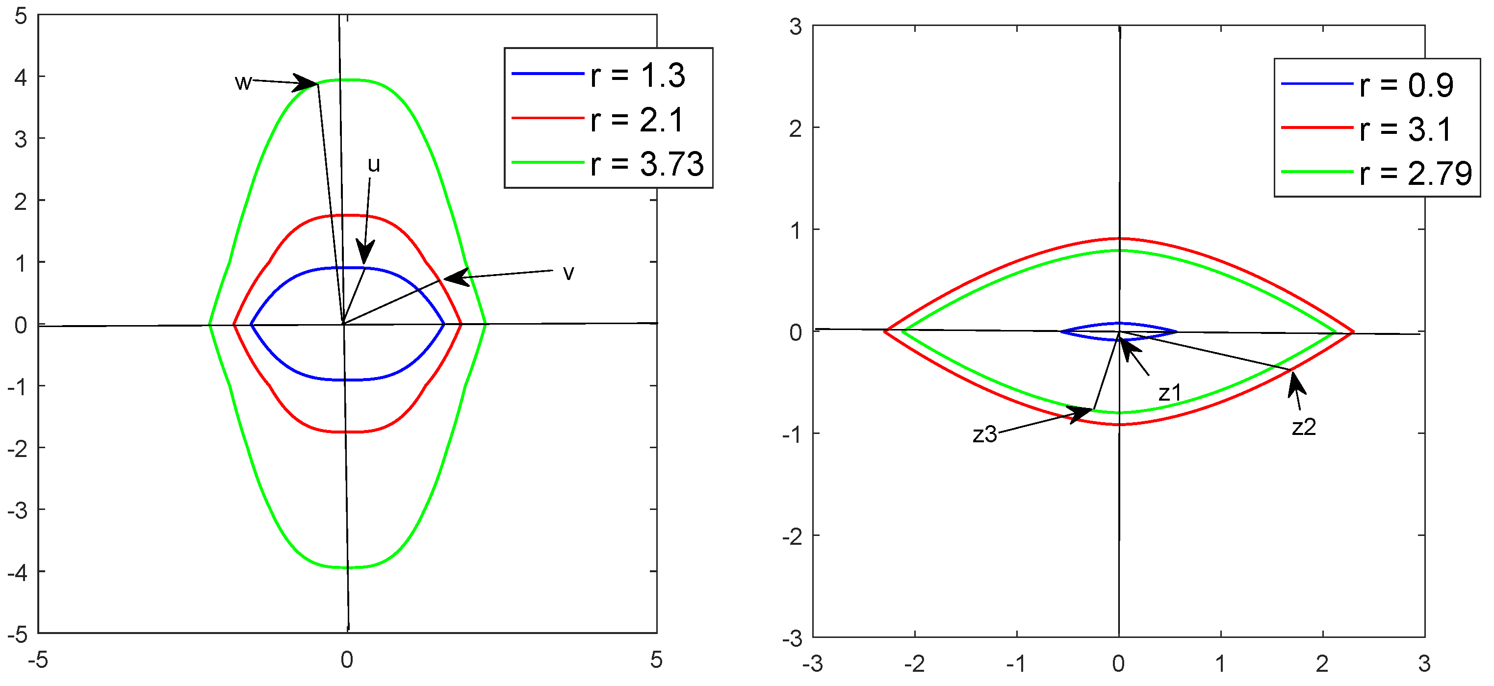
denote a “$[p,q]$-circle” of “$[p,q]$-radius” r and

$$D_{p,q}\left(r\right)=diag(r^{1/p},r^{1/q})$$

a specific diagonal matrix. Because of

$$C_{[p,q]}\left(r\right)=D_{p,q}\left(r\right)C_{[p,q]}\left(1\right),r>0,$$

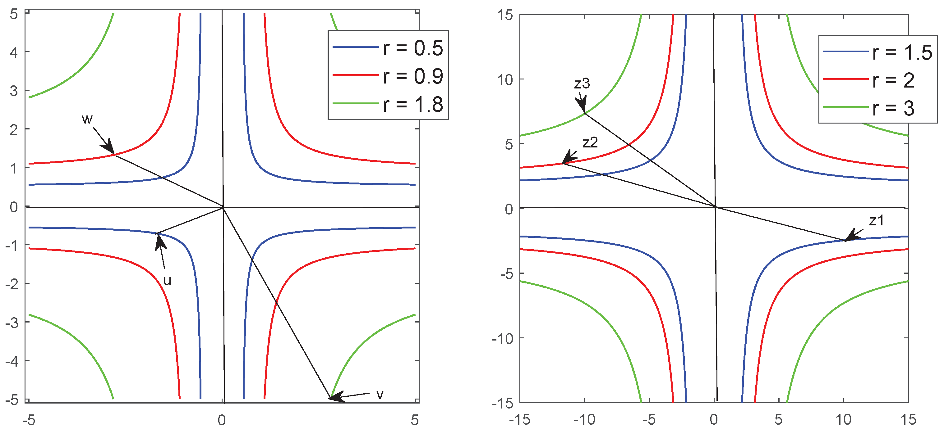
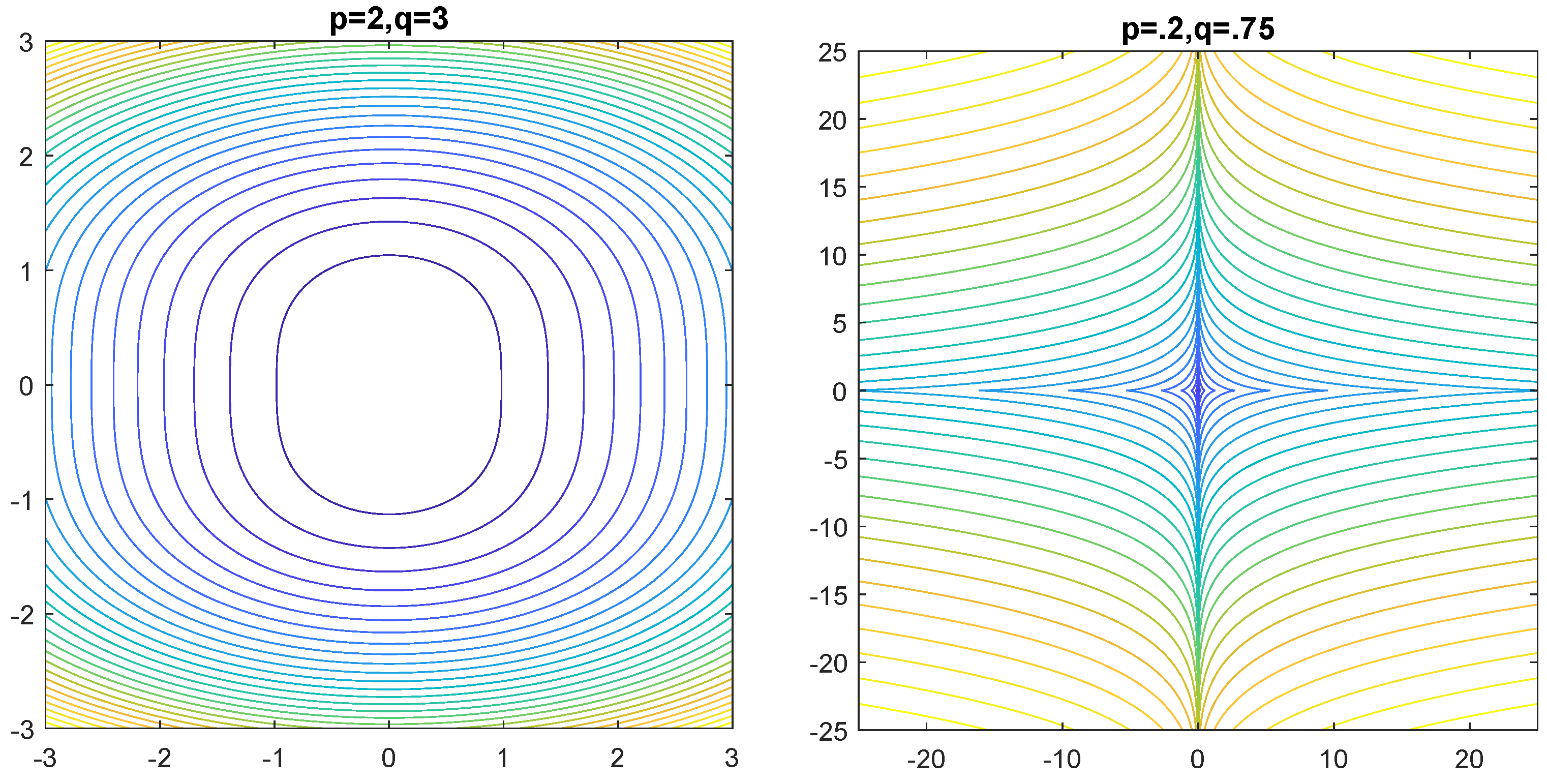
the function ${\left|(.,.)\right|}_{[p,q]}:{(x,y)}^T\to {\left|{(x,y)}^T\right|}_{[p,q]}$ is called matrix homogeneous. Figure 9 and Figure 10 show level sets $C_{[p,q]}\left(r\right)$ of the function ${\left|(.,.)\right|}_{[p,q]}$ for various values of $[p,q]$ and r.

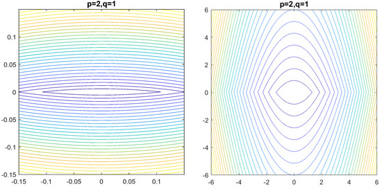
Figure 9. $[p,q]$-circles $C_{[p,q]}\left(r\right)$ for smaller and larger $[p,q]$-radii show change of shape and orientation as r changes.

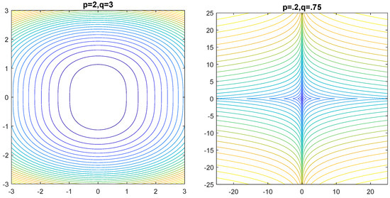
Figure 10. $C_{[p,q]}\left(r\right)$ for various values of $[p,q]$ and running $[p,q]$-radius r.

Due to change of shape of $C_{[p,q]}\left(r\right)$ as r changes we call $\{C_{[p,q]}\left(r\right),r>0\}$ a dynamic family of $[p,q]$-circles. Corresponding $l_{p,q}$-circle numbers are normalizing constants of certain probability density generating functions.

Definition 9.

We define the $[p,q]$-circle related vector multiplication, or $[p,q]$-vector multiplication, for short, of $z_1=Po{l}_{[p,q]}(r_1,{\phi }_1)$ by $z_2=Po{l}_{[p,q]}(r_2,{\phi }_2)$ as

$$z_1{\odot }_{[p,q]}{z}_2=Po{l}_{[p,q]}(r_1{r}_2,{\phi }_1+{\phi }_1).$$

For a graphical illustration of this vector multiplication, see Figure 11.

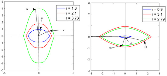
Figure 11. Vector $[p,q]$-products $w=u{\odot }_{[3,0.7]}v$ and $z3=z1{\odot }_{[1.7,0.3]}z2$.

Theorem 4.

The $[p,q]$-vector multiplication of $z_1=Po{l}_{[p,q]}(r_1,{\phi }_1)$ by $z_2=Po{l}_{[p,q]}(r_2,{\phi }_2)$ allows the analytical representation $z_1{\odot }_{[p,q]}{z}_2={(V,W)}^T$ with

$$V=\xi {\left(p|z_1{|}_{[p,q]}{\left|z_2\right|}_{[p,q]}\right)}^{1/p}{\left(\frac{|z_1{|}_2{\left|z_2\right|}_2}{|z_1{\odot }_2{z}_2{|}_{pq}}\right)}^q,W=\eta {\left(q|z_1{|}_{[p,q]}{\left|z_2\right|}_{[p,q]}\right)}^{1/q}{\left(\frac{|z_1{|}_2{\left|z_2\right|}_2}{|z_1{\odot }_2{z}_2{|}_{pq}}\right)}^p$$

and

$$\xi =sign(1-{\gamma }_1{\gamma }_2)\frac{|1-{\gamma }_1{\gamma }_2{|}^q}{{\left[(1+{\gamma }_1^2)(1+{\gamma }_2^2)\right]}^{q/2}}and\eta =sign({\gamma }_1+{\gamma }_2)\frac{|{\gamma }_1+{\gamma }_2{|}^p}{{\left[(1+{\gamma }_1^2)(1+{\gamma }_2^2)\right]}^{p/2}}$$

where

$${\gamma }_k=sign\left(x_k{y}_k\right){\left(\frac{p}{q}\right)}^{1/\left(pq\right)}\frac{|y_k{|}^{1/p}}{|x_k{|}^{1/q}},k=1,2.$$

Proof. 

It follows from Definition 9 that both

$$|z_1{\odot }_{[p,q]}{z}_2{|}_{[p,q]}=|z_1{|}_{[p,q]}{\left|z_2\right|}_{[p,q]}$$

and

$$|z_1{\odot }_{[p,q]}{z}_2{|}_{[p,q]}=\frac{|z_1{|}_{[p,q]}{\left|z_2\right|}_{[p,q]}}{N_{pq}^{pq}({\phi }_1+{\phi }_2)}\left(\right|cos({\phi }_1+{\phi }_2){|}^{pq}+|sin({\phi }_1+{\phi }_2){|}^{pq}).$$

Because the vector product of usual complex numbers allows the representation

$$z_1{\odot }_2{z}_2=|z_1{|}_2{\left|z_2\right|}_2\left(\begin{array}{c}cos({\phi }_1+{\phi }_2)\\ sin({\phi }_1+{\phi }_2)\end{array}\right)$$

it follows that

$$|z_1{\odot }_{[p,q]}{z}_2{|}_{[p,q]}=\frac{|z_1{|}_{[p,q]}{\left|z_2\right|}_{[p,q]}}{N_{pq}^{pq}({\phi }_1+{\phi }_2)}\frac{|z_1{\odot }_2{z}_2{|}_{pq}^{pq}}{|z_1{|}_2^{pq}{\left|z_2\right|}_2^{pq}}.$$

Thus,

$$N_{pq}({\phi }_1+{\phi }_2)=\frac{|z_1{\odot }_2{z}_2{|}_{pq}}{|z_1{|}_2{\left|z_2\right|}_2}$$

(19)

and

$$z_1{\odot }_{[p,q]}{z}_2=\left(\begin{array}{c}|z_1{\odot }_2{z}_2{|}_{pq}^{-q}{\left(p{r}_1{r}_2\right)}^{1/p}|z_1{|}_2^q{\left|z_2\right|}_2^q·\xi \\ |z_1{\odot }_2{z}_2{|}_{pq}^{-p}{\left(q{r}_1{r}_2\right)}^{1/q}|z_1{|}_2^p{\left|z_2\right|}_2^p·\eta \end{array}\right)$$

with $r_k={\left|z_k\right|}_{[p,q]},k=1,2$ and

$$\xi =sign(cos({\phi }_1+{\phi }_2))|cos({\phi }_1+{\phi }_2){|}^q,\eta =sign(sin({\phi }_1+{\phi }_2)){|sin({\phi }_1+{\phi }_2)|}^p.$$

Standard relationships for trigonometric functions ultimately provide the result. □

The following remark is an immediate consequence of this proof.

Remark 4.

For every $r>0,$ the set of transformations

$$\left(\begin{array}{c}x\\ y\end{array}\right)\to \left(\begin{array}{c}x\\ y\end{array}\right){\odot }_{[p,q]}zwhere{\left|z\right|}_{[p,q]}=1$$

builds the Lie group on the $[p,q]$-circle $C_{[p,q]}\left(r\right)$.

We additionally note that the $[p,q]$-radii of $z_1, z_2$ and $z=z_1{\odot }_{[p,q]}{z}_2$ satisfy the equation $r=r_1{r}_2,$ that is

$$\frac{{\left|x\right|}^p}{p}+\frac{{\left|y\right|}^q}{q}=\left(\frac{|x_1{|}^p}{p}+\frac{|y_1{|}^q}{q}\right)\left(\frac{|x_2{|}^p}{p}+\frac{|y_2{|}^q}{q}\right).$$

(20)

The following definition summarizes our consideration.

Definition 10.

For every pair of positive real numbers p and q with $p\ne q,$ we call the algebraic structure $({\mathbb{R}}^2,\oplus ,{\odot }_{[p,q]},·)$ the $[p,q]$-dynamic complex plane.

6. Invariant Probability Densities

A probability density $\varphi$ defined in ${\mathbb{R}}^2$ is said to be invariant with respect to transformation $T:{\mathbb{R}}^2\to {\mathbb{R}}^2$ if it satisfies the equation

$$\varphi \left(T(x,y)\right)=\varphi (x,y)\mathrm{for}\mathrm{all}{(x,y)}^T\in {\mathbb{R}}^2.$$

Invariant densities have interesting stochastic properties which, however, are outside the scope of the present work. Instead, some basic geometric properties of such densities are disclosed here at hand of three examples in which we use the knowledge provided in Section 4 and Section 5.

Example 7.

Let $p\ne q$ satisfy $p>0$ and $q>0$. A $[p,q]$-spherical distribution is uniquely determined by the distribution of its generating variate R, say. Moreover, if a $[p,q]$-spherical distribution has a density ϕ then it is of the form $\varphi ={\varphi }_{g;[p,q]}$,

$${\varphi }_{g;[p,q]}(x,y)={C(g;[p,q])g\left(\right|(x,y)}^T{|}_{[p,q]}),{(x,y)}^T\in {\mathbb{R}}^2$$

where $g:[0,\infty )\to [0,\infty )$ is a density generating function satisfying

$$0<\underset{0}{\overset{\infty }{\int }}{r}^{1/p+1/q-1}g\left(r\right)dr<\infty$$

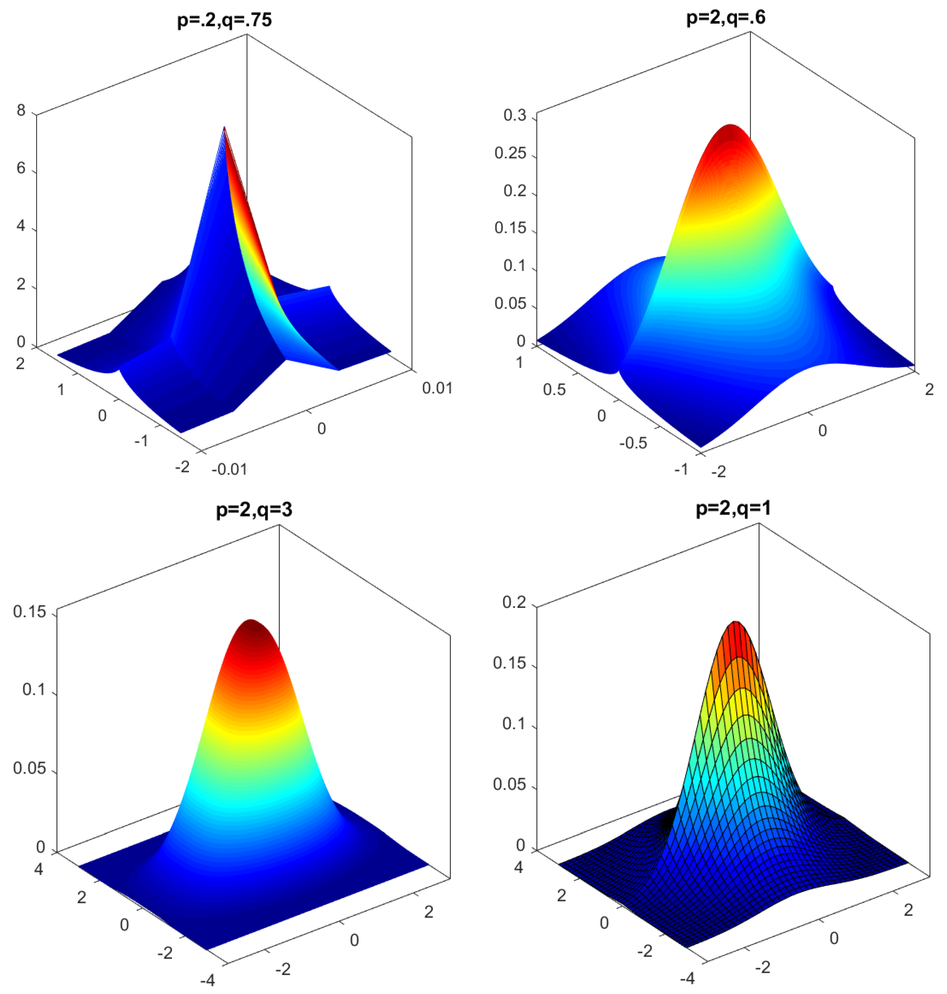
and $C(g;[p,q\left]\right)$ is a normalizing constant. The Gamma type density generating function is

$$g\left(r\right)=I_{[0,\infty )}\left(r\right)r^{N-1}{e}^{-\kappa r}.$$

With $g_0\left(r\right)=e^{-r},$ the density ${\varphi }_{g_0;[2,1]}$ is that of the two-dimensional Gauss–Laplace law which is a symmetrized variant of the Gauss-exponential distribution. More particular cases are Kotz type densities, power exponential densities, c.f. Figure 12, and Pearson type VII densities. Let z be any element from $C_{[p,q]}\left(1\right)$. Then, according to Section 5, the following invariance property holds,

$$\varphi \left(z{\odot }_{[p,q]}{(x,y)}^T\right)=\varphi \left({(x,y)}^T\right)forall{(x,y)}^T\in {\mathbb{R}}^2.$$

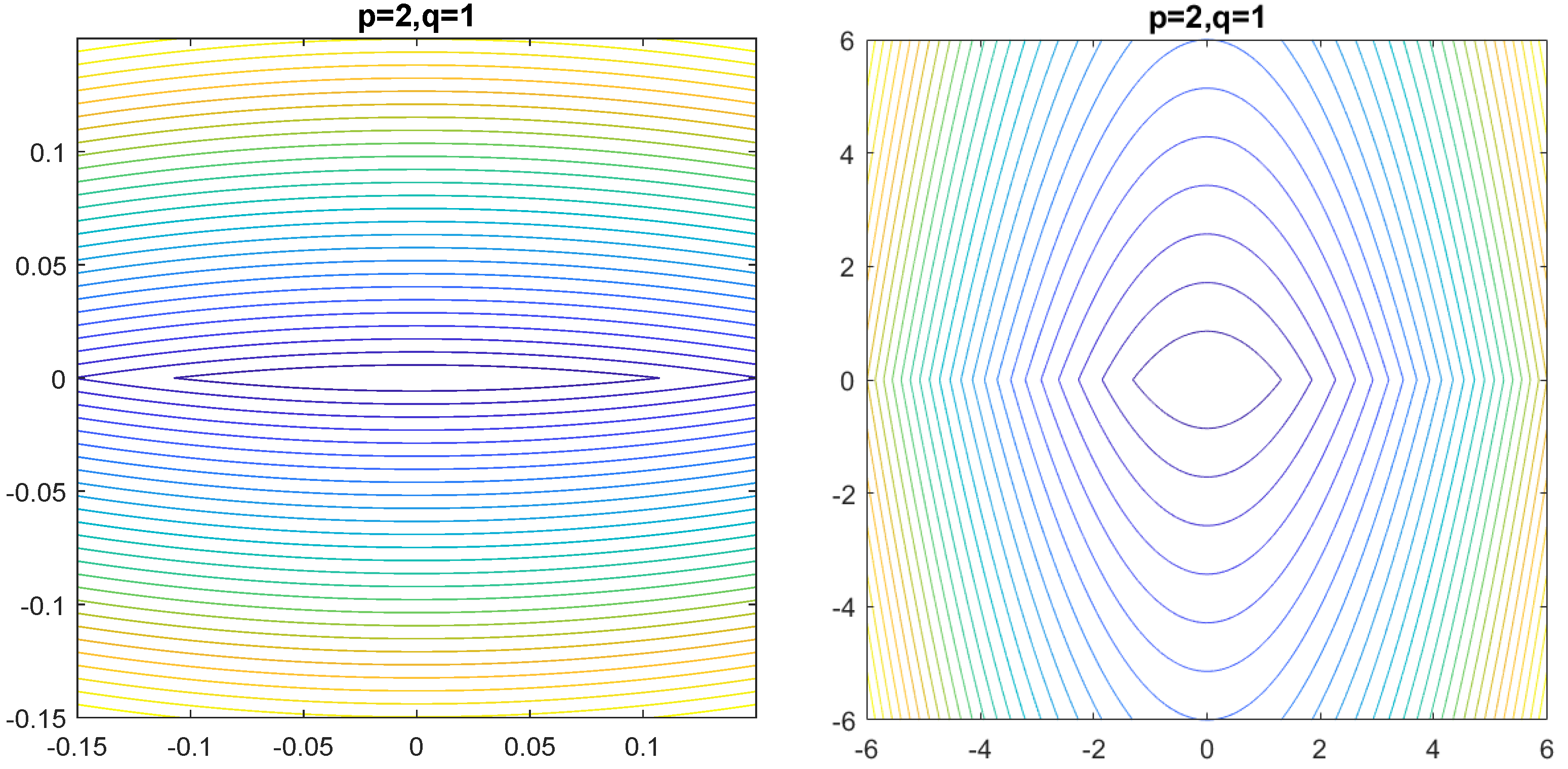
Figure 12. Power exponential density $\varphi (x,y)=C_{[p,q]}·e^{-{\left|x\right|}^p/p-{\left|y\right|}^q/q}$ for particular values of $[p,q]$.

Example 8.

Let $a>0,b>0$ and $\varphi ={\varphi }_{g;(a,b)}$ denote an axes-aligned $(a,b)$-elliptically contoured probability density,

$${\varphi }_{g;(a,b)}(x,y)={C(g;(a,b))g\left(\right|(x,y)}^T{|}_{(a,b)}),{(x,y)}^T\in {\mathbb{R}}^2.$$

If $z\in E_{(a,b)}\left(1\right)$ then, according to Section 4,

$$\varphi \left(z{\odot }_{(a,b)}{(x,y)}^T\right)=\varphi \left({(x,y)}^T\right)forall{(x,y)}^T\in {\mathbb{R}}^2.$$

Example 9.

Let $p>0$ and assume we are given a function $g:{\mathbb{R}}^{+}\to {\mathbb{R}}^{+}$ and a constant $C_{p,g}$ such that $\varphi ={\varphi }_{g,p}$ is an $l_{2,p}$-symmetric density in ${\mathbb{R}}^2$,

$${\varphi }_{g,p}(x,y)=C_{p,g}·{g\left(\right|x|}^p+{\left|y\right|}^p),(x,y)\in {\mathbb{R}}^2.$$

According to [6] , for any $z\in {\mathbb{R}}^2$ with ${\left|z\right|}_p=1$,

$$\varphi \left(z{\odot }_p{(x,y)}^T\right)=\varphi \left({(x,y)}^T\right)\mathrm{for}\mathrm{all}{(x,y)}^T\in {\mathbb{R}}^2.$$

7. Concluding Remarks

One of the empirical discoveries of the sixteenth century by Cardan was that although the system of equations $a·b=40,a+b=10,$ has no solution with real numbers a and b, formal setting $a=5+\sqrt{-15}$, $b=5-\sqrt{-15}$ and accepting the usual rules nevertheless seems to provide a solution. There are five axioms needed for developing a mathematical theory that reflects this observation in a completely strong way. First of all, one must assume that one can give an explanation for the formal symbol or quantity $\sqrt{-1}$. Furthermore one assumes that positive homogeneity $\sqrt{-x}=\sqrt{x}\sqrt{-1},x>0$ holds for the new symbol or number $\sqrt{-x}$ and that the formal sum $x+y\sqrt{-1}$ is explained. Finally, the product $(a+b\sqrt{-1})(c+d\sqrt{-1})$ should be explained formally as in calculating with real numbers, but using the equation $\sqrt{-1}·\sqrt{-1}=-1$. The first axiom ensures that not a whiff of mysticism or a lack of pedantry remains so that the existence of a tangible mathematical structure in which $\sqrt{-1}$ is explained is guaranteed. In the third axiom the addition of qualitatively different elements x and $y\sqrt{-1}$ should be explained.

The current concrete realizations of abstract complex algebraic structures satisfy all of these axioms, as shown in Section 2. Three new complex algebraic structures or complex planes are introduced in Section 3, Section 4 and Section 5. An application in the study of an advanced invariance property of certain probability densities is presented in Section 6.

All figures in this paper are drawn using Matlab.

References

- Ebbinghaus, H.-D.; Hermes, H.; Hirzebruch, F.; Koecher, M.; Mainzer, K.; Neukirch, J.; Prestel, A.; Remmert, R. Numbers; Springer: Berlin/Heidelberg, Germany, 1991. [Google Scholar]
- Mallik, A. The Story of Numbers; World Scientific Publishing: Singapore, 2018. [Google Scholar]
- Krasnov, M.A.; Kiselev, A.; Shikin, G.M.E. Mathematical Analysis for Engineers; Mir Publishers: Moscow, Russia, 1990; Volume I. [Google Scholar]
- Hieber, M. Analysis I; Springer Spektrum: Berlin/Heidelberg, Germany, 2018. [Google Scholar]
- Schmid, H. Elementare Technomathematik; Springer Spektrum: Berlin/Heidelberg, Germany, 2018. [Google Scholar]
- Richter, W.-D. On lp-complex numbers. Symmetry 2020, 12, 877. [Google Scholar] [CrossRef]
- Richter, W.-D. Three-complex numbers and related algebraic structures. Symmetry 2021, 13, 342. [Google Scholar] [CrossRef]
- Shuster, J.A.; Koeplinger, J. Elliptic complex numbers with dual multiplication. Appl. Math. Comput. 2010, 216, 3497–3514. [Google Scholar] [CrossRef]
Publisher’s Note: MDPI stays neutral with regard to jurisdictional claims in published maps and institutional affiliations. |
© 2021 by the author. Licensee MDPI, Basel, Switzerland. This article is an open access article distributed under the terms and conditions of the Creative Commons Attribution (CC BY) license (https://creativecommons.org/licenses/by/4.0/).