Factors of Bottom Sediment Variability in an Abandoned Alkaline Waste Settling Pond: Mineralogical and Geochemical Evidence

Abstract

The aim of this study is to determine the characteristics of the chemical and mineral composition of sediment layers in a technogenic settling pond. This pond is located on urban land in Berezniki (Perm Krai, Russia), outside the territory of operating industrial facilities, and contains alkaline saline industrial wastes. The origin of this waste was related to sludge from the Solvay soda production process, which had been deposited in this pond over a long period of time. However, along with the soda waste, the pond also received wastewater from other industries. As a result, the accumulated sediment is characterized by variation in morphological properties both in depth and laterally. Five undisturbed columns were taken to study the composition of the accumulated sediment. The obtained samples were analyzed by X-ray diffraction (XRD), synchronous thermal analysis (STA), and X-ray fluorescence (XRF) analysis. The results showed that the mineral composition of bottom sediments in each layer of all studied columns is characterized by the predominance of calcite precipitated from wastewater. Along with calcite, due to the presence of magnesium and sodium in the solution, other carbonates precipitated—dolomite and soda (natron), as well as complex transitional carbonate phases (northupite and trona). Together with carbonate minerals, the chloride salts halite and sylvin, sulfate minerals gypsum and bassanite, and pyrite and nugget sulfur were established. The group of terrigenous mineral components is represented by quartz, feldspars, and aluminosilicates. The chemical composition of sediments in the upper part of the section generally corresponds to the mineral composition. In the lower sediment layers, the role of amorphous phase and non-mineral compounds increased, which was determined by the results of thermal analysis. The content of heavy metals and metalloids also increases in the middle and lower sediment layers. When categorized according to the Igeo value, an excessive degree of contamination (class 6) was observed in all investigated columns for copper content (Igeo 5.2–6.1). Chromium content corresponds to class 5 (Igeo 4.1–4.6), antimony to class 4 (Igeo 3.0–4.0), and lead, arsenic, and vanadium to classes 2 and 3 (moderately polluted and highly polluted). The data obtained on variations in the mineral and chemical composition of sediments represent the initial information for the selection of methods of accumulated waste management.

1. Introduction

A comprehensive mineralogical-geochemical study of bottom sediments in water bodies can provide extensive information about their history [1]. Sediment formation involves both authigenic mineral precipitation processes and external particle input, resulting in distinctive terrigenous-evaporite sequences that preserve a depositional ‘record’ within their layers [2,3,4].

Of particular research interest are sediments from highly mineralized (hypersaline) alkaline aquatic systems. Such environments typically develop in endorheic (closed) basins where evaporation exceeds precipitation [5,6]. Thus, natural alkaline lakes serve as unique natural laboratories for studying low-temperature mineral precipitation and the distribution of chemical elements between solution, gas, and mineral phases [7].

A critical aspect of mineralogical studies of saline lakes is the investigation of carbonate equilibria and crystallization pathways of carbonate minerals [8]. The precipitation and deposition of CaCO₃ can be of fundamental importance to the biogeochemistry of lacustrine ecosystems due to its linkages with the cycles of other components, such as dissolved organic carbon and suspended particulate matter. Moreover, this process may regulate sedimentation rates in lakes [9,10,11].

The ratios of terrigenous components to authigenic minerals also serve as an imprint of the sedimentation history in water bodies. It is noteworthy that even silicate minerals can have an authigenic origin in alkaline lake environments. Under alkaline and hypersaline conditions with Na-dominated solutions, authigenic silicates can crystallize as hydrous silica phases (e.g., kerolite, magadiite) [7,12].

Although scientific research on natural hypersaline alkaline sites is relatively diverse, much less attention has been paid to sediments from man-made water bodies. Meanwhile, alkaline industrial waste can concentrate useful components [13,14]. At the same time, technogenic saline alkaline environments can pose a hazard to the environment. When alkaline filtrate seeps into aquifers, the composition of the water changes. This can include an increase in pH, a depletion of dissolved oxygen, and an increase in sulfate load and heavy metal concentrations [15,16]. This is particularly relevant in regions with humid climates where saline alkaline bodies of water are not naturally formed and the resulting sediments pose an environmental hazard. The composition of wastewater and its impact can be unique to each case, depending on the effluent composition and local conditions, unlike natural objects. For example, a study of alkaline drainage from steel slag landfills in the UK revealed significant variations in pH, hydrochemical facies, and trace element content across a small area [15]. In Silesia, Poland, researchers studied 45 ponds, finding pH values ranging from strongly acidic to alkaline (pH 2.4–9.6) [17].

Industries contributing to the formation of hypersaline alkaline water bodies primarily include the extraction and processing of highly soluble salts, as well as the chemical industry. Inorganic alkaline industrial wastes exhibit diverse mineral compositions but are universally characterized by carbonates, oxides, hydroxides, silicates, aluminates, and/or aluminosilicates of Na, Ca, K, and/or Mg, which dissolve or hydrate to generate alkalinity [16,18,19]. Such wastes are generated during paper, cement, and lime production, metallurgy and metal processing, coal combustion, and other industrial activities [19]. Alongside high alkalinity (pH > 9), many industrial wastes are also highly saline. This is particularly true for chromium production waste [20], bauxite residue (red mud) from alumina production [21], and especially Solvay-process soda ash waste [21,22,23,24,25].

The wastewater from soda ash production primarily consists of a calcium chloride solution containing calcium hydroxide particles. This solution mixes with impurities from saltwater purification and limestone calcination, resulting in an alkaline liquid with pH > 11.5 that contains dissolved calcium chloride, sodium chloride, and suspended particles such as calcium carbonate, sulfates, magnesium hydroxide, and calcium hydroxide. These Solvay-process effluents are directed to settling ponds (lagoons), where solid particles settle, and the liquid is discharged into rivers and lakes [22,26]. Thus, soda sludge settling ponds serve as unique incubators for mineral precipitation from calcium-saturated chloride brines. The sediment accumulated over decades of production in such reservoirs reaches tens of meters in thickness [25,27,28], clearly indicating sedimentation rates significantly exceeding those in natural environments.

The alkaline and saline conditions can create favorable environments for preserving impurities and other waste materials that enter these reservoirs. Active industrial waste reservoirs typically receive effluents of relatively homogeneous composition, which is determined solely by the parameters of the feedstock and the processing technologies. However, uncontrolled wastewater discharge may introduce extraneous substances. An example of such a site was investigated in this study.

The settling pond of the soda plant in Berezniki (Russia) was built in a low-lying area during the Soviet era and was used as a reserve tank for discharging and settling distillation liquid during the construction of the main sludge storage. However, even after the main production reservoir was commissioned, the reserve pond remained a buffer tank for a long time, discharging industrial effluent along with soda ash production waste. In addition, this pond was hydraulically connected to the open sewer of industrial effluent, which discharged effluent from several plants. As a result of the mixing of distillation liquid with effluents of various compositions, including those from metallurgical plants and organic synthesis plants, the pond accumulated many meters of bottom sediments. With a general dominance of calcium carbonate and an alkaline pH (>10), the sediment has distinct layers, each with its own unique characteristics [29].

Following the dissolution of the Soviet Union and subsequent industrial restructuring, this temporary storage facility became municipal property, falling outside the jurisdiction of existing companies, and now requires remediation. Proper remediation design necessitates detailed characterization of each sediment layer’s geochemical and mineralogical properties, with due regard to the possibilities and restrictions dictated by the accumulated material.

Therefore, the objective of this study is to determine the chemical and mineral composition features of sediment layers in this anthropogenic settling pond. It is hypothesized that layer-by-layer analysis of the technogenic deposits may reconstruct the sediment formation history, depositional conditions, temporal variations in wastewater composition, and other factors influencing sediment formation. Furthermore, the accurate identification of the sediment composition will provide crucial insights for developing effective remediation strategies.

2. Materials and Methods

2.1. Description of the Study Site

The study site is located in Berezniki, a city in the Perm Krai region of Russia, within the Verkhnekamskoe (Upper Kama) salt deposit area. In addition to the extraction and processing of potash salts, the production of soda ash is a major industrial activity in the area. Soda ash has been produced here since 1883 using the Solvay ammonia-soda process, which utilizes brines from the Verkhnekamskoe deposit and carbonate rocks as raw materials.

The pond containing the accumulated sediments has an almost regular pentagonal shape and is surrounded by dams. It has a diameter of approximately 500 m and a surface area of 170,000 square meters. The water depth varies seasonally but typically does not exceed 1 m. Throughout its existence, the primary sources of water input have been atmospheric precipitation and wastewater discharges. Wastewater entered the pond from the eastern and western sides, though discharge has now been completely discontinued. No visible hydrological connection to other water bodies exists. Approximately 150 m west of the pond lies the shoreline of the Kama River (Kama Reservoir), which serves as the main water supply source for the region.

2.2. Sediment Sampling Methodology

Before sampling, the depth of the sediment was examined using a rigid feeler made from a leveling rod. The thickness of the pasty sediment was measured until the hard bottom was reached. The sediment thickness was measured at 74 evenly distributed points on a 50 × 50 m grid, as well as directly at the sampling locations.

Five undisturbed core samples were collected using a specialized coring device equipped with 110 mm diameter plastic tubes to investigate the sediment composition [30]. The sampling locations corresponded to the cardinal directions (north, east, south, and west) and the center of the pond (C) (Figure 1).

The conditions and sampling apparatus of all columns were identical. The W and E cores were obtained in September 2024, the N and S cores were obtained in March 2025, and data for the C core were derived from earlier sampling conducted in March 2022. Each coring tube featured a plastic check valve to maintain sediment integrity during retrieval. All sampling equipment components were constructed from chemically inert materials and thoroughly cleaned prior to use to prevent contamination (e.g., rust particles or other foreign matter) in the collected samples.

Prior to sampling, the depth of the sediment at the drill hole was determined with a rigid, labeled dipstick. The sediment was partially compacted during extraction. To reconstruct the true thickness of each layer, the thickness of the sediment after extraction was adjusted to the thickness determined by the dipstick using a proportional method.

The layers of sediment cores from each extraction point were then described, had their thicknesses measured, and were photographed. Sediment layers were identified by visual characteristics (color, layering, and small inclusions) and morphological features (consistency and porosity).

2.3. Sample Preparation and Laboratory Analysis Methods

The mineral composition of the samples was investigated by X-ray diffraction (XRD) to determine the presence of crystalline phases in them and their diagnosis using a powder diffractometer XRD D2 Phaser (Bruker, Germany), equipped with an X-ray tube with a copper anode (emitting CuKα, λ = 1.54060 Å), a generator with a voltage of 30 kV and a current of 10 mA, a linear detector LYNX EYE, and a Ni-filter. Imaging conditions were as follows: divergent slit of 0.6 mm, Soller slits primary of 2.5°, secondary of 2.5°; angular range of 2θ from 5 to 70°; pulse set frequency at each point of 1.0 s; step of 0.03. Curve processing (smoothing, peak search), qualitative analysis, and semi-quantitative analysis were performed using Diffrac.Eva version 1.2 software. The PDF-2 powder diffractometry database [2010 edition] was used to search for mineral phases. Quantitative analyses were performed using Topas version 4-2 software. Reference-free analysis was carried out on the basis of the Rietveld method—a procedure for minimizing the deviation between the experimental and theoretically calculated diffractograms. Only the content of the crystalline part of the rock was determined, and the sum of mineral phases was brought to 100%.

The following methods of thermal analysis were also used to study the samples synchronously combined within one experiment: differential scanning calorimetry (DSC), based on the registration of thermal effects accompanying physical transformations and chemical reactions occurring with the substance during heating; thermogravimetric (thermo-weight) analysis (TGA), based on obtaining and studying the patterns of changes in the mass of the substance during heating. The main results of the thermal analysis are thermal curves (heating curves)—thermograms—which allow us to quantitatively evaluate the main processes occurring with the substance during heating and provide additional information on the forms of elements, including the amorphous phase. Experimental studies were carried out on the synchronous thermal analyzer STA 409 PC Luxx from Netzsch-Geratebau GmbH (Selb, Germany). The samples, after grinding, were placed in a corundum crucible and heated to a temperature of 1200 °C at a rate of 30 °C per minute. The samples were investigated in a dynamic gas atmosphere using Ar (gas flow rate of 10 mL/minute for the weighing system, and 20 mL/minute for the measuring chamber).

To determine the chemical composition of bottom sediments, X-ray fluorescence analysis was carried out on a BRUKER (Rheinstetten, Germany) S8 Tiger Sequential Wave Dispersion Spectrometer. During sample preparation, the determination of loss on ignition (LOI) was carried out. For this purpose, a rock sample was calcined for one hour at a slow temperature increase to a constant mass at a temperature of 1000 °C, then cooled in the desiccator and weighed to the 4th decimal place. The calcination and weighing were repeated until a constant mass was obtained. The calcination was carried out using a high-temperature electric furnace PL 10/12.5 (NakalProm, Moscow, Russia).

The preparation of samples for the determination of elements in oxide form included grinding to a particle size of 10 µm in a Pulverisette 6 monomill (Fritsch, Idar-Oberstein, Germany). Then, a sample of the abraded sample (0.8 g) was thoroughly mixed with flux in the ratio of 1:10 and fused on a K1 Prime material fusion system with pre-installed Katanax K1 Prime software. For the determination of trace elements, a portion of the ground sample (2 g) was thoroughly mixed with wax at a ratio of 4:1. Under pressure of 20 t on the hydraulic laboratory press VANEOX 25t PR-25A-HD (FLUXANA GmbH&Co.KG, Bedburg-Hau, Germany), a tablet with a diameter of 40 mm on a boric acid substrate was produced from the obtained mixture. The measurement was carried out using a program of quantitative chemical analysis for silicate rocks, created according to calibration charts on Russian-made standards.

These analytical studies were carried out in the Nanomineralogy Sector of the Perm State University Center for Collective Use, which is accredited in accordance with the requirements of the international ISO 17025 standard [31]. The Center provides mandatory QC/QA applications in analytical methods, including standard application, instrument calibration, metrological equipment verification, sample preparation methods, and the required number of control measurements.

The results of the study of the physicochemical properties of the aqueous extract (pH, alkalinity), as well as the total content of oil products and organic carbon, are drawn from the materials of the study conducted in September 2021. The conditions and apparatus for experimental work are described in detail in the publication [29].

2.4. Data Processing Methods

Principal component analysis (PCA) was performed in RStudio 2024.12.0 Build 467, using an inbuilt function of the R programming language, prcomp(). The prcomp() function uses Singular value decomposition (SVD), which examines covariance/correlations between individuals, just like the PCA () function from the FactoMineR package [32]. SVD, according to the R help, has better numerical accuracy. Therefore, prcomp() is preferred over princomp(). Redundancy analysis (RDA) was performed to evaluate the relationship between the mineral composition and chemical composition of the slurries using the RDA function of the vegan package for R [33].

3. Results

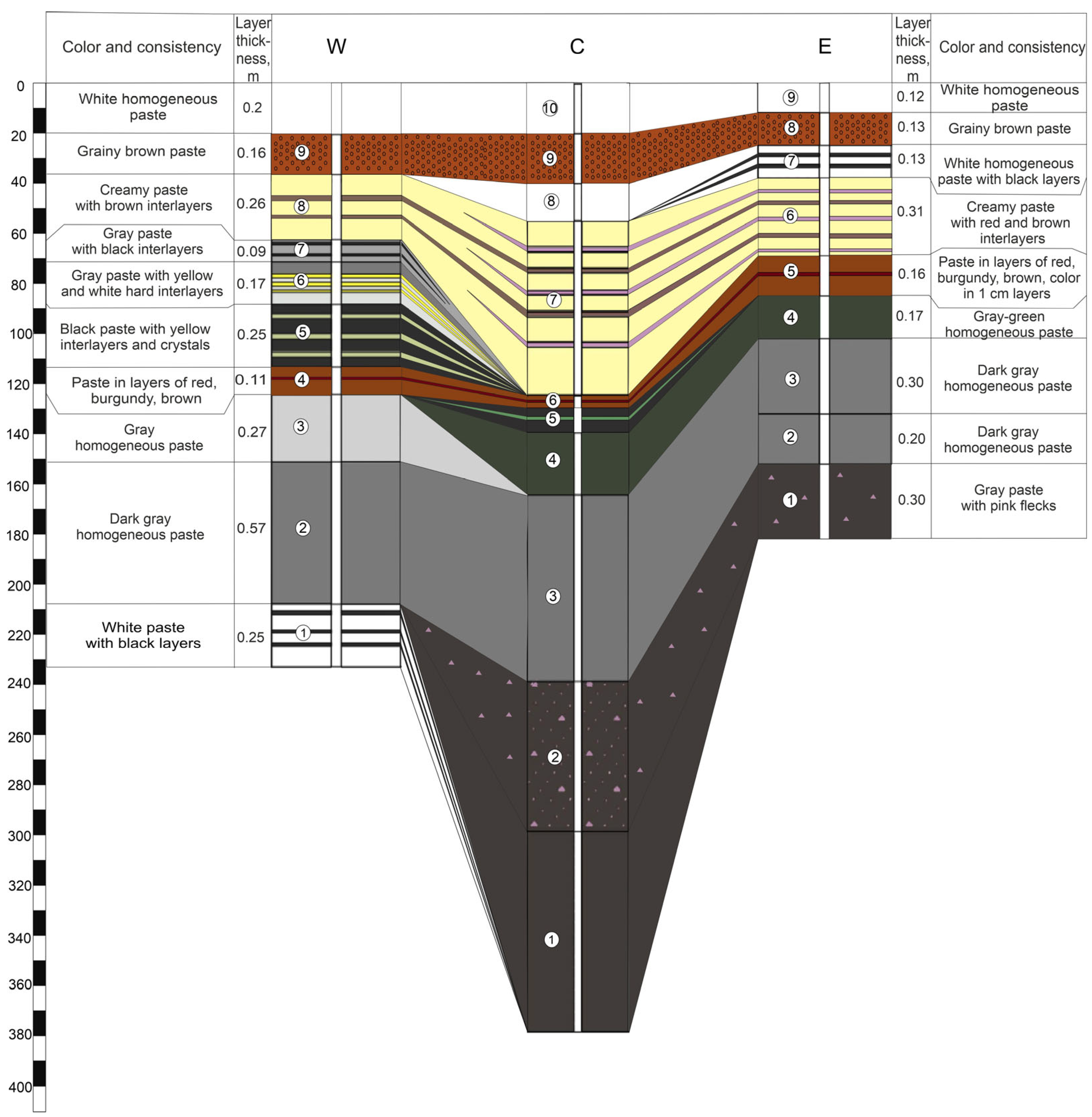
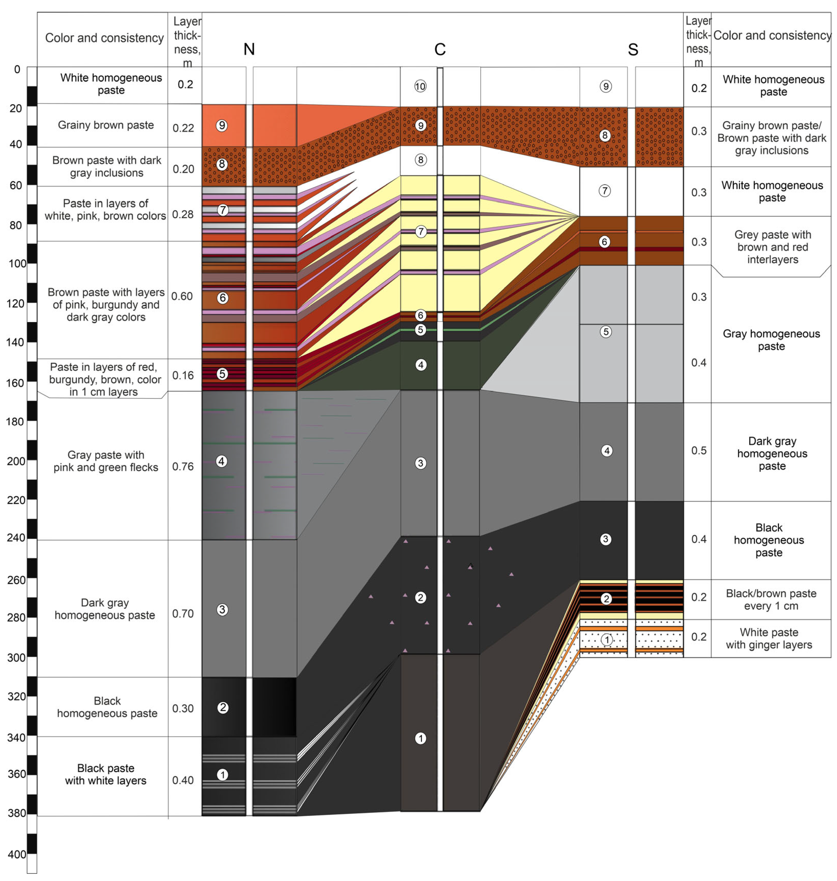
3.1. Description of the Physical Parameters of the Sediments

During the drilling of five sediment columns, the sediment thickness ranged from 182 to 380 cm. The consistency of all sediments was homogeneous paste-like, except for isolated yellow crystals observed in the middle section of core W. Additionally, the brown sediment layer in the upper part of the cores exhibited a porous, granular texture. Each core typically contained 9–10 distinct layers, varying significantly in color (from white and cream to deep black). The stratigraphic sequence of sediment layers along the W–C–E and N–C–S transects is illustrated in Figure 2 and Figure 3. The upper white layer in cores W, N, and S is shown schematically. This layer was identified during the site inspection, but an undisturbed sample could not be collected during drilling.

In the upper part (down to ~1 m depth), the color change pattern was similar in all cores (white → brown → white → cream with interlayers), suggesting similar depositional conditions over most of the study area. Below 1 m depth, significant variability in sediment physical properties (color, odor, and consistency) was observed in core W (western portion) where distinct bright yellow interlayers alternated uniformly with a light gray sediment matrix. As noted above, some of the yellow interlayers consisted of crystals up to 1.5–2 cm in diameter. The total thickness of the sediment with yellow interlayers reached 20 cm. At comparable depths in the central (N, C, S) and eastern (E) cores, a layer of vivid red to burgundy sediment (up to 16 cm thick) was identified, adjacent to a 10–17 cm thick layer of intense green sediment.

The underlying sediments were predominantly gray to black. In the W core, white sediment with black laminations was encountered below a gray homogeneous matrix at depths greater than 2 m. In the northern core N, gray paste-like sediment (below the “colored” layers) contained thin pink and green laminations. In cores C and E, a layer of pink particle inclusions was observed below the homogeneous gray mass. The deepest layers (>2 m) of the southern core S showed light-colored layers similar to those in the western core W.

3.2. Mineral Composition of the Sediments

According to X-ray phase analysis, the mineral composition of the crystalline phase of bottom sediments is characterized by the predominance of carbonate minerals (Figure 4).

All diffractograms of the investigated sediment layers have a high background and an absence of peaks at small angles. This indicates the presence of X-ray amorphous matter. The results of the thermal (DSC/TG) analysis confirm this conclusion. According to the results of the analysis, the characteristic effect observed in the high-temperature range for the studied sediments is the thermal decomposition of carbonate compounds. This process occurs regardless of the perfection of the crystal structure of the substance and is accompanied by heat absorption and mass loss. The calculated data from the thermal analysis of the carbonate content (based on mass loss within the range of carbonate decomposition, which is the main sedimentary phase) are similar to the X-ray phase analysis data, but only for the samples from the top part of the studied columns (layers W9, W8, W7, W6, E9, and E7) (see Figure 5). For the other studied layers, the carbonate content is significantly lower, which indicates the presence of amorphous phase or non-mineral compounds. The results obtained confirm the complexity of solving the problem of estimating the forms of elemental findings for objects such as technogenic sediments.

The calcite content of the crystalline phase in the samples studied varies from 39.9% to 88.4%. This mineral is formed by fine precipitation from the liquid phase of pulp, which is a waste at the ammonia method of soda production [34]. Together with calcite, due to the presence of magnesium and sodium in the solution other carbonates, dolomite CaMg(CO₃)₂ and soda Na₂CO₃∙10H₂O (natron), as well as complex transitional carbonate phases nortupite Na₃Mg(CO₃)₂Cl and trona Na₃H(CO₃)₂·2H₂O, were precipitated (Figure 6). On average, the crystalline phase of all the studied samples contains 71% carbonate minerals (

Table 1. Generalized data on mineral composition of sediments (crystalline part) based on the results of X-ray phase analysis, wt.%.

		Σcarb.	ΣAl-Si	ΣS	ΣCl	Portlandite
W	M	66.6	4.7	5.1	18.3	3.3
	σ	6.9	4.1	4.4	7.9	3.1
	Cv	10.3	88.7	87.0	43.2	94.2
N	M	73.6	9.5	2.8	12.1	-
	σ	9.8	10.4	0.6	3.4	-
	Cv	13.3	110.3	21.6	28.3	-
S	M	70.7	11.4	5.5	9.2	-
	σ	9.8	4.4	1.8	3.0	-
	Cv	13.8	38.9	33.1	32.9	-
E	M	74.2	2.7	7.6	12.8	0.8
	σ	9.9	1.5	4.4	7.2	0.4
	Cv	13.3	55.2	58.5	56.5	53.5
All samples	M	71.2	7.1	5.3	13.1	-
	σ	9.3	6.8	3.5	6.5	-
	Cv	13.0	96.5	67.8	49.6	-

Notes: M—calculated average content per column, σ—standard deviation, CV—coefficient of variation, %; Σcarb.—sum of carbonate minerals (calcite, dolomite, soda, etc.); ΣAl-Si.—sum of aluminosilicate minerals (feldspars, clays, quartz); ΣS—sum of sulfur minerals (gypsum, pyrite, bassanite, sulfur); ΣCl—sum of chloride minerals (halite, sylvin).

).

The second most common group of minerals in the crystalline part of the studied sediments are chloride salts: halite (NaCl) and sylvin (KCl). On average, they accounted for 13% of the mineral composition of all studied samples. The presence of these minerals indicates the initial brines from which the sediment formed were highly mineralized. Additionally, saturated chloride brines are a component of the distillation liquid used in the production of soda by the Solvay method [30].

Among the sulfur mineral compounds identified in the crystalline part of the studied sediments were gypsum (Ca₂SO₄·2H₂O) and semi-aqueous calcium sulfate hydrate bassanite (Ca₂SO₄·0.5H₂O) (Figure 7). Pyrite (FeS₂) and nugget sulfur (S) were also found in a number of layers. On average, sulfur compounds accounted for 5% of the mineral composition of the studied samples.

The group of terrigenous mineral components in the crystalline phase of sediments includes quartz, feldspar, and aluminosilicate minerals. The influx of these minerals is likely connected to the influx of sand, dust, and clay, which are carried by wind and washed off by rain from the surrounding area. On average, the content of terrigenous minerals in the studied samples was 7%.

The variation of mineral composition by depth within each column is visualized in Figure S1. Taking into account the peculiarities of the mineral composition of the northern N column, we observe that layer N7 contains a high proportion of terrigenous minerals (up to 36%). In the western part of the pond (column W), in addition to the typical carbonate minerals—dolomite and soda—it is characterized by the presence in rather large amounts (up to 7%) of the mineral portlandite—calcium hydroxide (Figure 8). This mineral can also precipitate from solution under strongly alkaline conditions. In layer W6, both individual crystals and solid yellow interlayers up to 1 cm thick were found, consisting of 86% portlandite.

A specific feature of the sediment in the eastern column E is the maximum calcite content (up to 88% in the upper layers E9 and E7). The peculiarity of column E sediments is the high content of bassanite. Its maximum content is observed in layer 8%–10% and in the lower layers E1–E3—7%–11% (Figure 9). In layers E9 and E5–E7, its content is low and amounts to 0.7%–4%. Gypsum content is up to 3%.

The mineral composition of sediments of the southern column S is also characterized by the predominance of carbonate minerals (calcite up to 76%, dolomite up to 4.1%, and soda up to 9.3% in layer S5). Among sulfur compounds, gypsum dominates (1.5%–8.3%), while pyrite and bassanite were not detected. Nugget sulfur (up to 5.3%) was observed in the middle and lower layers.

3.3. Chemical Composition of the Sediments

According to the results of X-ray fluorescence analysis, the content of the main rock-forming elements in each of the layers of the five columns was determined.

Table 2. Content of main rock-forming elements according to XRF results, wt.%.

		CaO	Fe2O3	SO3	MgO	SiO2	Na2O	Al2O3	K2O	MnO	TiO2	P2O5	Cl	LOI
W	M	28.1	1.5	7.2	3.0	5.6	5.2	1.3	3.1	0.3	0.9	0.04	9.2	34.6
	σ	7.2	1.1	4.0	2.0	2.8	1.4	1.0	1.4	0.2	0.8	0.01	2.3	4.0
	Cv	25.8	73.5	55.1	67.4	49.9	26.8	77.5	46.2	89.5	85.2	31.8	25.2	11.5
N	M	42.0	2.4	3.0	4.1	4.7	2.1	1.2	0.5	0.5	1.5	0.04	12.6	25.5
	σ	3.7	0.9	0.9	1.2	1.8	0.5	0.5	0.2	0.2	1.0	0.01	2.1	2.5
	Cv	8.8	37.7	28.6	28.9	38.8	23.3	38.7	42.7	48.4	66.2	23.1	16.5	9.7
C	M	43.1	2.1	2.7	3.6	4.7	1.7	1.1	0.6	0.4	1.4	0.03	11.6	26.9
	σ	5.8	0.9	0.7	2.0	2.5	0.9	0.5	0.4	0.2	1.0	0.01	4.1	5.4
	Cv	13.5	43.3	27.4	56.6	52.1	50.9	47.9	59.0	62.2	68.1	45.3	35.7	20.1
S	M	42.1	3.2	3.3	3.7	5.3	1.5	1.4	0.9	0.5	1.7	0.05	8.1	28.7
	σ	8.2	1.4	0.6	1.1	3.1	0.5	0.7	0.5	0.3	1.4	0.01	1.2	4.2
	Cv	19.5	45.7	19.6	30.7	59.0	33.0	52.3	50.5	55.6	81.6	30.6	15.4	14.8
E	M	28.5	1.8	6.4	4.6	6.1	3.3	1.7	0.3	0.3	1.2	0.04	13.7	32.2
	σ	8.9	1.1	2.6	3.3	3.1	0.8	1.0	0.2	0.3	0.7	0.01	4.7	5.1
	Cv	31.2	64.3	41.1	70.9	51.5	24.7	58.8	53.2	105.4	64.5	35.1	34.5	15.8

Notes: M—mean content, σ—standard deviation, C_V—coefficient of variation, %.

shows descriptive statistical parameters of the content of components. The variability of the content of each component within the investigated column is assessed by calculating the coefficient of variation (Cv).

The leading shares in the composition of each sediment layer in all columns are occupied by calcium oxide (CaO), as well as by losses during LOI (loss on ignition) calcination (including carbon dioxide released during the thermal destruction of carbonate minerals, chemically bound water, organic matter, and some chlorine and sulfur oxides) (Figure 10).

The samples with the highest proportion of calcium correspond to the columns located along the central axis (N, C, and S). LOI shows inverse dynamics of change along the pond lateral. The highest LOI values are found in columns E and W.

Taking into account the fact that LOI mainly consists of CO₂ when calcium carbonate (the main sediment component) is destroyed, discrepancies in the average LOI and CaO content across the pond area indicate an increased input of chlorine, sulfur oxides, and organic matter in the western and eastern parts of the site.

The third most widespread component of the sediment composition is chlorine. Its average content increases from west and south (8.1 wt.%–9.2 wt.%) to east and north (11.6 wt.%–13.7 wt.%). The content of sulfur compounds (SO₃) and LOI increase in the western and eastern parts of the pond, about 2 times higher than in the central columns. The specificity of sediment composition from the western part of the site (by column W) consists of a higher content of sodium and, especially, potassium oxides.

The general trends of chemical composition change with depth can be seen in Column C, equidistant from the sources of previous wastewater discharge. Our analyses of Figure 11 show a decrease in potassium and chlorine content from the lower to the upper layers. The maximum magnesium content occurs in the middle interval of the section. The content of Al₂O₃, SiO₂, Fe₂O₃, TiO₂, and MnO in the upper layers changed under the influence of single factors. For the other columns, these trends are also true, taking into account the greater contrast of compositional changes in columns W and S, located in the area of former sewage discharge. The variation of sediment composition by depth in columns N, E, S, and W is shown in Figure S2.

Based on the XRF results from layer samples of each core, we compiled a comprehensive database incorporating oxide weight percentages, loss on ignition (LOI), and sampling depths. These data were subjected to principal component analysis (PCA). Prior to analysis, all concentration data were log-transformed for normalization. The analysis identified two principal components (PCs) that collectively explain 61.2% of the total variance (PC1 = 42.7%, PC2 = 18.5%). The results were visualized using the ggbiplot package in R, displaying variable vectors and sample groups (cores) on a biplot (Figure 12).

Based on the results of the data analysis, the following general regularities are highlighted. The variability of chemical composition within each column is determined mainly by the first principal component PC1, while the variability between columns is determined by the second principal component (see the orientation of group-ovals along the X-axis).

According to the second principal component, three groups of columns are distinguished, corresponding to their spatial position: the westernmost (W), easternmost (E), and a group of columns located in the center of the pond, away from the sources of wastewater inflow (N, C, S).

By analyzing the vectors of variables, we can identify the components of the material composition of the solid phase of the sediments, the content of which in the solid phase of the sediments is mutually correlated. Thus, the contents of silicon, phosphorus, and aluminum oxides correlate with each other and with the first principal component PC1. Chlorine, titanium, and magnesium oxide can be identified in another similar group. The content of manganese (by MnO) and iron (by Fe₂O₃) increases with increasing sampling depth, with an inverse correlation of the content of these components being observed in comparison with the loss on ignition (LOI). The contents of potassium and sodium oxides are closely related to each other and also correlate with the sulfur content (by SO₃), and all of them together with the second major component of PC2.

Based on the figure, it is assumed that the variability in PC1 is determined by the variation in the amount of impurities (silicon, phosphorus, aluminum, titanium, and magnesium), while the variability in PC2 is related to the variation in alkalinity and salinity.

3.4. Trace Element Composition of Sediments

According to the results of X-ray fluorescence analysis, the content of trace components (Sc, V, Cr, Co, Ni, Cu, Zn, Ga, As, Rb, Sr, Y, Zr, Nb, Sn, Sb, Cs, Ba, La, Ce, Pb, Th, and U) in each sediment layer from five studied columns was determined. When normalizing the detected concentrations by the average values characteristic of the upper part of the continental crust (UCC) [35], a list of components with elevated contents in the studied samples (more than 2UCC on average per column) was determined. Descriptive statistical parameters of the content of these components are given in

Table 3. Content of trace elements according to XRD results, ppm.

		Sc	V	Cr	Ni	Cu	As	Nb	Sb	Ba	Pb
W	M	13.6	361	1490	37.7	1650	11.5	77.0	6.2	843	133
	σ	10.5	290	1060	27.3	1670	4.6	58.7	2.5	647	86.0
	Cv	77.3	80.3	71.1	72.3	101	39.5	76.2	40.4	76.7	64.8
	M/UCC	1.9	6.8	42.4	2.0	116	5.8	3.0	20.1	1.3	7.8
	Igeo	−0.4	1.5	4.2	0	5.2	1.8	0.2	3.6	−1	2.1
N	M	15.5	366	1570	36.5	1670	12.8	75.8	6.0	2250	113
	σ	6.3	186	840	14.3	782	3.0	37.9	2.4	1830	80.2
	Cv	40.3	50.7	53.5	39.2	46.9	23.4	50.1	40.8	81.2	70.8
	M/UCC	2.2	6.9	44.9	2.0	117	6.4	2.9	19.2	3.4	6.7
	Igeo	0.4	1.9	4.6	0.3	6.1	2.1	0.6	3.2	0.8	1.9
C	M	13.0	322	1350	48.5	2060	13.0	74.1	5.2	1610	132
	σ	7.8	159	705	45.4	2190	2.7	46.9	1.2	1580	76.2
	Cv	60.2	49.3	52.4	93.6	107	20.5	63.3	23.6	98.0	57.8
	M/UCC	1.9	6.1	38.4	2.6	144	6.5	2.9	16.8	2.4	7.8
	Igeo	0.3	1.8	4.4	0.3	5.8	2.1	0.5	3.4	−0.5	2.2
S	M	14.2	420	1490	37.4	1430	13.9	73.7	9.1	1760	145
	σ	10.5	249	961	16.5	1220	5.1	53.5	6.8	1190	95.9
	Cv	73.7	59.3	64.6	44.1	84.9	36.8	72.5	74.6	67.8	66.3
	M/UCC	2.0	7.9	42.5	2.0	100	6.9	2.8	29.4	2.6	8.5
	Igeo	0.6	2.0	4.1	0.3	5.5	2.1	0.2	4.0	0.1	2.3
E	M	14.7	396	1620	35.8	1520	11.5	88.9	4.1	1090	167
	σ	9.8	242	1160	21.2	1360	3.2	62.0	1.4	711	150
	Cv	66.8	61.3	71.7	59.3	89.3	28.1	69.7	35.1	65.1	90.2
	M/UCC	2.1	7.5	46.3	1.9	107	5.7	3.4	13.1	1.6	9.8
	Igeo	0.1	1.9	4.5	0	5.5	1.9	0.7	3.0	−0.4	2.3

Notes: M—mean content, σ—standard deviation, C_V—coefficient of variation, %, M/UCC—ratio of mean content to UCC data [35], Igeo [36].

. Additionally, to assess the level of sediment contamination by the listed elements, the Igeo index was calculated [36]. The average elemental contents in the upper part of the continental crust [35] were used as background in the Igeo calculation.

When normalized to UCC values, the highest enrichment factors in the studied sediments were observed for antimony (13.1–29.4), chromium (38.4–46.3), and copper (100.1–143.8). Vanadium, arsenic, and lead contents exceeded UCC averages by 6–10 times, while scandium, nickel, niobium, and barium showed 2–3× enrichment.

The distribution of concentrations of the above trace components by sediment depth is considered in the example of column C, located in the center of the studied pond and equidistant from possible sources of polluted effluents. The profiles of trace component content are shown in Figure 13.

Antimony and arsenic are most uniformly distributed along the depth. The content of scandium in the samples is also relatively uniform, except for layer C8 in the upper part of the column, where its concentration decreases several times. Nickel and copper concentrations change in a very similar way: a gradual increase from the lower layers to the C5 layer with a gradual decrease to the upper part of the section. Chromium, lead, niobium, vanadium, and barium are characterized by higher concentrations in the lower layers, a decrease in layers C4 and C5, an increase in layers C6–C8, and a further decrease towards the top of the section. The variation of trace components in sediment composition with depth in columns N, E, S, W is shown in Figure S3.

The PCA biplot of trace elements (Figure 14) revealed two principal components (PCs) that collectively account for 67.1% of the total variance (PC1 = 45.9%, PC2 = 21.2%). Our analysis of variable vectors identified trace elements with statistically correlated concentrations in the sediment solid phase. Thus, the content of vanadium and scandium correlates with each other and the principal component PC1. The contents of antimony and barium correlate positively with each other and negatively with the principal component PC2. The contents of arsenic, copper, and nickel are rather closely correlated with each other.

The combined PCA biplot with data on basic oxide composition and trace elements (Figure 15) gives us an idea of the relationship between trace elements and sediments of different compositions. For example, lead content correlates with sediments with increased potassium, sodium, and sulfur content (column W). Increased concentrations of vanadium and scandium are associated with an increase in the proportion of terrigenous components (aluminum, silica), copper, and nickel—with an increase in chlorine content. Increased concentrations of barium and manganese are observed in the lower layers of the sediment.

4. Discussion

4.1. Regularities of Changes in the Material Composition of Sediments

Analysis of the chemical and mineral composition of sediments accumulated in an abandoned settling pond indicates that their formation was predominantly governed by the precipitation of solid-phase residues from Solvay-process soda production wastewater. As shown above, CaO, Cl, and LOI, among other things including carbon dioxide from carbonate decomposition, are the leading components of the chemical composition of each sludge layer. The mineralogical composition is consistent with the chemical data, being chiefly represented by calcite, with subordinate contributions from other carbonates and gypsum. These findings exhibit strong concordance with published descriptions of Solvay-process soda ash waste composition [22,26] and correlate closely with analytical data from sludge deposits in adjacent operational containment facilities of soda production plants [37,38,39], as well as with analogous deposits documented internationally [25,27].

Furthermore, sedimentological investigations revealed discernible variability in physical properties, particularly color and consistency. Geochemical and mineralogical analyses confirm that this heterogeneity is attributable to compositional variations within the sediment matrix.

To identify the driving forces behind the variability in sediment chemical composition, redundancy analysis (RDA) was performed in R. Potential predictors (factors influencing compositional variability) included sampling depth (depth) and physicochemical parameters of aqueous extracts from corresponding sediment layers, as reported in [29]: pH, alkalinity, total organic content (organic), and mass concentration of petroleum products (petroleum). The triplot correlation diagram derived from the analysis is presented in Figure 16.

Our analysis of the plot highlights trends consistent with prior findings from sediment chemical composition data and PCA results. Variability in sediment composition along RDA1 is primarily driven by pH and petroleum product content, while RDA2 reflects variations in total organic content.

Elevated petroleum product concentrations were observed in the lower layers of all studied sediment cores and appear to be spatially consistent across the pond. Visually, this is evidenced by the dark black coloration of deeper sediment layers (see Figure 2 and Figure 3). The presence of petroleum-saturated layers (containing crude oil and fuel oil) may be attributed to historical discharges from fuel tank cleaning operations, which ceased after local boiler houses transitioned to natural gas. Due to the antiquity of these events, the highest petroleum concentrations coincide with the deepest sections of the pond basin.

Additionally, deeper sediment layers exhibit higher proportions of terrigenous mineral components (identified as quartz, feldspars, and clay particles) compared to the middle and upper layers. The decrease in terrigenous input can be traced back to the construction of the dams around the study pond, the transition of the site from a natural discharge area to an artificial storage facility, and the effect of gravitational differentiation.

Another distinctive feature of the deep and middle sediment layers in the central part of the pond (cores N, S) is their higher manganese and titanium content compared to the western and eastern sections. Within the studied reservoir, these elevated concentrations can be attributed to the mixing of Solvay-process distiller waste (calcium-saturated) with metal-rich wastewater discharges.

As noted previously, the western and eastern sections of the pond, which received wastewater inflows, exhibit distinct sediment composition characteristics. The most alkaline layers with the lowest petroleum product content correspond to the western core W. These sediments also demonstrate the highest proportions of potassium and sodium. The mineralogical description provided above indicates that potassium and sodium in the western pond section were fixed as chloride salts (halite and sylvite).

Furthermore, the middle sediment layers of core W (W6–W7) show the maximum portlandite content, which remains stable under high pH conditions and in the absence of atmospheric contact. Upon exposure to atmospheric CO₂, portlandite undergoes carbonation and is replaced by calcite crystals [40,41]. Collectively, this evidence suggests that sediments in the western pond section formed primarily through the inflow of saline, highly alkaline wastewater.

The eastern section of the pond was located in the overflow zone of an open industrial drainage canal that collected wastewater from several industrial facilities. While this overflow was later eliminated, it previously received wastewater from soda production. During the Soviet era, acidic effluents from neighboring industries (a non-ferrous metals plant and an organic synthesis plant) were added to the alkaline soda production waste for neutralization. As a result, the sediments in the eastern core E contain higher levels of total organic matter, while titanium and magnesium oxides make up a larger proportion of the elemental composition. Soda ash distillate entering the pond from this side also resulted in elevated chlorine concentrations in core E sediments.

In addition, the sediments in eastern core E contain the highest proportion of bassanite (calcium sulfate hemihydrate)—the primary precipitation phase preceding gypsum formation, a characteristic mineral of distillate sediments [42,43].

4.2. Trace and Toxic Elements in Sediments

Our analysis of trace element compositions in the sediments revealed several elements exhibiting the highest enrichment levels. These include copper (an enrichment ratio of the mean column content to Upper Continental Crust (UCC) reference values = 100.1–143.8), chromium (38.4–46.3), antimony (13.1–29.4), lead (6.7–9.8), vanadium (6.1–7.9), and arsenic (5.7–6.9). Mean concentrations of scandium, nickel, niobium, and barium exceeded UCC geochemical background values by factors of 1.3–3.4.

When assessing potential ecological risks from metal loads, the highly alkaline environment (pH > 10) characteristic of the study site must be considered. Under alkaline conditions, most elements exhibit reduced mobility and become immobilized in sediments. However, certain elements forming oxyanions remain mobile at high pH, particularly Cu, As, Cr, and V [17,19].

Pollution classification based on the geoaccumulation index (Igeo) follows seven categories [36]:

• Class 0: Igeo ≤ 0—practically uncontaminated.
• Class 1: 0 < Igeo ≤ 1—uncontaminated to moderately contaminated.
• Class 2: 1 < Igeo ≤ 2—moderately contaminated.
• Class 3: 2 < Igeo ≤ 3—moderately to strongly contaminated.
• Class 4: 3 < Igeo ≤ 4—strongly contaminated.
• Class 5: 4 < Igeo ≤ 5—strongly to extremely contaminated.
• Class 6: 5 < Igeo—extremely contaminated.

According to this classification (Table 3), all sediment cores showed extreme contamination (Class 6) for copper (Igeo 5.2–6.1). Chromium levels corresponded to Class 5 (Igeo 4.1–4.6) and antimony to Class 4 (Igeo 3.0–4.0), while lead, arsenic, and vanadium ranged between Classes 2 and 3 (moderately to strongly contaminated). Scandium, nickel, niobium, and barium concentrations did not indicate contamination based on Igeo values.

To determine the origin of trace elements in the sediments, mean metal and metalloid concentrations across the study site were compared with several reference datasets. These included composite data from studies of ammonia-soda white sludge in China [44]; legacy soda production waste deposits in Jaworzno, Poland [45]; and trace element concentrations in the depositional environment (soil) of the Verkhnekamskoye deposit area, representing local atmospheric deposition [46].

Additionally, metal concentrations were compared with analytical data from studies of wastewater sediments in the lower reaches of the industrial discharge channel in Berezniki [47]. This channel collects effluents from multiple industrial facilities, with treated wastewater being discharged into the Kama Reservoir after settling in its estuarine section. The abandoned pond under investigation is located in the upper course of this very channel. The comparative results are presented in

Table 4. Comparison of average trace element concentrations of the study pond with data on soda waste, local soils, sewage sludge, and regulations for use of sludge in reclamation.

	Studied Water Body (Mean Value)	Sewage Sludge from Berezniki Industrial Canal [47]	Spoil Heaps in Jaworzno, Poland [45]	Soda Sludge, China [44]	Soils of the Verkhnekamskoye Field [46]	RF Norms for Technical Reclamation [48]
V	373	-	-	-	78	-
Cr	1500	84.8	6.24	20.6	152	2000
Ni	39.2	34.2	2.35	7.81	31	800
Cu	1670	33.0	-	37.9	-	1500
As	12.5	1.62	-	3.63	6.3	40
Sb	6.12	0.18	-	-	-	-
Ba	1510	54.7	-	-	-	-
Pb	138	18.1	46.89	10.4	15.2	1000

.

As evidenced by Table 4, the studied pond sediments exhibit significant enrichment of all analyzed trace elements when compared both with fresh and legacy wastes from Solvay-process soda production and with background concentrations in local soils. However, certain elements show concentrations comparable to local geochemical background levels. For instance, the mean nickel content in the abandoned pond sediments (39.18 mg/kg) only slightly exceeds average values for soils in the Verkhnekamskoye deposit area (31 mg/kg) [46].

The comparison with data from the lower reaches of the industrial discharge channel [46], where all analyzed elements show substantially lower concentrations than in the studied pond, may indicate reduced anthropogenic pressure during the current operational period compared to the sediment formation phase.

The additional comparison with Russian regulatory limits for soil reuse in technical reclamation projects [48] suggests that, for the analyzed components, the sediments could potentially be used for earthworks. Only copper content showed a minor exceedance (approximately 11%) of the regulatory threshold.

When interpreting these mean concentrations, it is critical to recognize the highly heterogeneous vertical distribution of metals and metalloids within the sediment column, emphasizing the need to identify the most toxic intervals. Analysis of the depth-dependent distribution patterns (Figure 13 and Figure S3) reveals a clear stratification:

-

Arsenic and antimony show peak concentrations in deeper layers with a gradual upward decrease (cores W, S, and N) or relatively uniform distribution (cores C, E).

-

Vanadium, chromium, and lead show increasing concentrations from deep to intermediate layers, followed by a decrease toward the surface.

-

Notable concurrent depletion of V, Cr, and Pb occurs in layers N6, W6, E7, and S8, with subsequent enrichment in overlying layers.

-

Copper (with the highest UCC enrichment factors) follows a similar distribution pattern to V, Cr, and Pb, but reaches maximum concentrations in deeper layers (C5, W5, and E5) coinciding with the depletion intervals of the other metals.

To determine the distribution patterns of trace elements in sediments, PCA was performed on a sample of trace elements, as well as on a combined sample of micro and macro components of sediments (Figure 14 and Figure 15). Looking at the PCA results in Figure 14, correlated groups of elements (Pb, Cr-Nb-V-Sc, As-Cu-Ni, and Sb-Ba) can be observed.

When considering the relationship between these groups and the main components of the sediment, the correlation of lead with sodium and sulfur compounds is noted. The highest concentrations of lead were recorded in the sediments of the eastern column E.

The distribution of chromium, niobium, vanadium, and scandium shows a positive correlation between themselves and components of the terrigenous group (Al₂O₃, SiO₂), as well as a negative correlation with CaO content. Thus, the accumulation of these trace components in the sediment may have occurred with a decrease in the input of soda distillate liquid into the study pond and a concomitant decrease in the deposition of calcium minerals. During the formation of this sediment, the proportion of organic wastewater (indirectly, this can be indicated by P₂O₅) and input from runoff from the adjacent area may have increased.

The group of trace elements As-Cu-Ni shows positive correlations with magnesium, iron, and chlorine, a negative correlation with losses during calcination, and the actual absence of correlation with CaO. Based on this relationship, we can assume the preferential input of As-Cu-Ni with chloride effluents of non-ferrous metallurgy enterprises, which entered the study pond together with the distillation liquid of the Solve technology until the mid-1990s.

Antimony and barium concentrations show the best correlation with manganese content and sampling depth. These components entered the sediment composition at the initial filling stage and may be related to the composition of oil and fuel oil, which determined the dark color of the first sediment layers.

4.3. Areas of Reclamation

When considering the prospects of reclaiming the territory where the abandoned pond is located, the following regulations should be taken into account. According to the current legislation of the Russian Federation, it is forbidden to locate waste accumulation facilities within the boundaries of a settlement, as well as within the water protection zone. Therefore, the reclamation of sludge by leaving it in place and covering it with an impermeable screen is impossible due to the conditions of its location. The removal, transportation, and disposal of such a large amount of contaminated sediments (more than 1,300,000 tons) is not possible due to the lack of available space in existing specialized landfills. It is therefore necessary to consider options for the treatment and utilization of the accumulated sludge.

Existing methods for the management of sewage sludge and, in particular, soda sludge, include dewatering of the sludge and its use as a soil acidity-reducing reclamation agent, as a binding agent for construction mixtures and construction materials, and as an anti-icing agent [24,44,49]. When choosing ways of handling sediments of the studied object, it is necessary to take into account the variability of its composition, which poses the additional tasks of studying the toxicity of layers and differentiated selection of technologies and directions of use.

In addition, the XRF analysis method used in this study does not allow the determination of the content of some potentially hazardous components, such as mercury. At the same time, the mercury content may be a significant limiting factor in the choice of soda sludge recycling [44].

Given the high pH and salinity values of the studied pond sediments, their direct use in agricultural operations may be dangerous. Taking into account the experience of handling similar sediments, as well as the high content of toxic trace elements in some sediment layers, a promising direction for their use may be the development of technologies for processing the sludge of the investigated object into construction and structural materials.

5. Conclusions

The results of the study of the material composition of saline alkaline sediments accumulated in an abandoned settling pond in Berezniki showed its complex structure. It has been established that the leading factor of sediment formation was the precipitation of solid particles (mainly calcite) from the wastewater of soda production using the Solvay method. This result is combined with historical information about the pond. However, unlike the usual industrial wastewater lagoons of the Solvay process, the study pond has been a receiver of wastewater from other plants over the years and has also undergone periodic changes in water level and composition. As a result of these factors, the sediments formed in the pond are characterized by a variety of layers with different physical properties (color, consistency, and odor) and material composition.

Studies have established the main regularities of changes in sediment composition by depth and length of the pond. Thus, the deepest sediment layers throughout the pond area are characterized by increased concentrations of oil products. These layers are black and gray in color. The specificity of the mineral composition of sediments of the lower layers consists of the increased share of terrigenous components (quartz and feldspars), which can be explained by the absence of barriers to the entry of terrigenous particles before the construction of dams surrounding the pond at the initial stage of its functioning, as well as by the gravitational differentiation of terrigenous components. The middle sediment layers are characterized by a decrease in the proportion of calcium, the main component of the distillation fluid, and an increase in magnesium, titanium, sulfur, sodium, and, in particular, trace elements (chromium, arsenic, copper, and lead). Presumably, this period of sludge accumulation is associated with the simultaneous input of wastewater from other surrounding industries, such as non-ferrous metallurgy, acids, alkalis, and organic synthesis products, with the distillation liquid from the Solvay production. These beds are characterized by the most varied sediments color (bright yellow, green, and red). In addition, they show the brightest differentiation in latitudinal direction, which indicates the different composition of wastewater from the eastern and western parts of the pond during this period. Later on, as the input of wastewater from third-party industries decreased, the intensity of sludge coloration decreased together with the concentrations of trace elements. The upper layers of the sediments are a white paste of calcium carbonate with few impurities.

The information obtained on the variations in the mineral and chemical composition of the sediments is the baseline information for the selection of methods for the management of accumulated waste. Necessary directions for further sludge research include the determination of the content of some hazardous toxicants not detected by XRF analysis (e.g., mercury), in-depth studies of the amorphous phase of sludge, and detailing the organic matter contained in the sludge. Together with the determination of the toxicity of the accumulated sludge to living organisms, this information will help to define both the limits and possibilities of the development of a remediation technology for the abandoned pond.

6. Patents

Vaganov S., Perevoshchikov R., Menshikova E., Ushakova E. Method for sampling bottom sediments for environmental studies and a device for its implementation. RU Patent 2762631, filed 21 June 2021, and issued 21 December 2021

References

1. Maltsev, A.E.; Leonova, G.A.; Bobrov, V.A.; Krivonogov, S.K. Geochemistry of Holocene Sapropels from Small Lakes of the Southern Western Siberia and Eastern Baikal Regions; Academic Publishing House «Geo»: Moscow, Russia, 2019; 445p. [Google Scholar] [CrossRef]
2. Strakhovenko, V.D.; Solotchina, E.P.; Goosl, Y.S.; Solotchin, P.A. Geochemical factors for endogenic mineral formation in the bottom sediments of the Tazheran lakes (Baikal area). Russ. Geol. Geophys. 2015, 56, 1437–1450. [Google Scholar] [CrossRef]
3. Solotchina, E.P.; Kuzmin, M.I.; Solotchin, P.A.; Maltsev, A.E.; Leonova, G.A.; Danilenko, I.V. Authigenic carbonates from holocene sediments of Lake Itkul (South of West Siberia) as indicators of climate changes. Dokl. Earth Sci. 2019, 487, 54–59. [Google Scholar] [CrossRef]
4. Solotchin, P.A.; Solotchina, E.P.; Maltsev, A.E.; Leonova, G.A.; Krivonogov, S.K.; Zhdanova, A.N.; Danilenko, I.V. Carbonate sedimentation in high -mineralized Lake Bolshoi Bagan (South of West Siberia): Dependence on holocene climate changes. Geol. Geophys. 2023, 64, 1318–1329. [Google Scholar] [CrossRef]
5. Saccò, M.; White, N.E.; Harrod, C.; Salazar, G.; Aguilar, P.; Cubillos, C.F.; Meredith, K.; Baxter, B.K.; Oren, A.; Anufriieva, E.; et al. Salt to conserve: A review on the ecology and preservation of hypersaline ecosystems. Biol. Rev. 2021, 96, 2828–2850. [Google Scholar] [CrossRef]
6. Liang, C.; Yang, B.; Cao, Y.; Liu, K.; Wu, J.; Hao, F.; Han, Y.; Han, W. Salinization mechanism of lakes and controls on organic matter enrichment: From present to deep-time records. Earth-Sci. Rev. 2024, 251, 104720. [Google Scholar] [CrossRef]
7. Raudsepp, M.J.; Wilson, S.; Morgan, B. Making Salt from Water: The Unique Mineralogy of Alkaline Lakes. Elements 2023, 19, 22–29. [Google Scholar] [CrossRef]
8. Raudsepp, M.J.; Wilson, S.; Zeyen, N.; Arizaleta, M.L.; Power, I.M. Magnesite everywhere: Formation of carbonates in the alkaline lakes and playas of the Cariboo Plateau, British Columbia, Canada. Chem. Geol. 2024, 648, 121951. [Google Scholar] [CrossRef]
9. Womble, R.N.; Driscoll, C.T. Calcium carbonate deposition in Ca2+ polluted Onondaga Lake, New York, USA. Water Res. 1996, 30, 2139–2147. [Google Scholar] [CrossRef]
10. Roche, A.; Vennin, E.; Bundeleva, I.; Bouton, A.; Payandi-Rolland, D.; Amiotte-Suchet, P.; Gaucher, E.C.; Courvoisier, H.; Visscher, P.T. The Role of the Substrate on the Mineralization Potential of Microbial Mats in A Modern Freshwater River (Paris Basin, France). Minerals 2019, 9, 359. [Google Scholar] [CrossRef]
11. Zeyen, N.; Benzerara, K.; Beyssac, O.; Daval, D.; Muller, E.; Thomazo, C.; Tavera, R.; López-García, P.; Moreira, D.; Duprat, E. Integrative analysis of the mineralogical and chemical composition of modern microbialites from ten Mexican lakes: What do we learn about their formation? Geochim. Cosmochim. Acta 2021, 305, 148–184. [Google Scholar] [CrossRef]
12. Armstrong, I.; Cury, L.F.; Titon, B.G.; Athayde, G.B.; Fedalto, G.; da Rocha Santos, L.; Soares, A.P.; de Vasconcelos Müller Athayde, C.; Manuela Bahniuk Rumbeslperger, A. The Occurrence of Authigenic Clay Minerals in Alkaline-Saline Lakes, Pantanal Wetland (Nhecolândia Region, Brazil). Minerals 2020, 10, 718. [Google Scholar] [CrossRef]
13. Gao, D.; Wang, F.-P.; Wang, Y.-T.; Zeng, Y.-N. Sustainable Utilization of Steel Slag from Traditional Industry and Agriculture to Catalysis. Sustainability 2020, 12, 9295. [Google Scholar] [CrossRef]
14. Li, G.; Liu, J.; Yi, L.; Luo, J.; Jiang, T. Bauxite residue (red mud) treatment: Current situation and promising solution. Sci. Total Environ. 2024, 948, 174757. [Google Scholar] [CrossRef]
15. Mayes, W.M.; Younger, P.L.; Aumônier, J. Hydrogeochemistry of Alkaline Steel Slag Leachates in the UK. Water Air Soil Pollut. 2008, 195, 35–50. [Google Scholar] [CrossRef]
16. Gomes, H.I.; Mayes, W.M.; Rogerson, M. Alkaline residues and the environment: A review of impacts, management practices and opportunities. J. Clean. Prod. 2015, 112, 3571–3582. [Google Scholar] [CrossRef]
17. Spyra, A.; Cieplok, A.; Kaszyca-Taszakowska, N. From extremely acidic to alkaline: Aquatic invertebrates in forest mining lakes under the pressure of acidification. Int. Rev. Hydrobiol. 2023, 108, 5–16. [Google Scholar] [CrossRef]
18. Xue, S.G.; Wu, Y.J.; Li, Y.W.; Kong, X.F.; Zhu, F.; William, H.; Li, X.F.; Ye, Y.Z. Industrial wastes applications for alkalinity regulation in bauxite residue: A comprehensive review. J. Cent. South Univ. 2019, 26, 268–288. [Google Scholar] [CrossRef]
19. Moyo, A.; Parbhakar-Fox, A.; Meffre, S.; Cooke David, R. Alkaline industrial wastes—Characteristics, environmental risks, and potential for mine waste management. Environ. Pollut. 2023, 323, 121292. [Google Scholar] [CrossRef]
20. Brito, E.M.S.; Piñón-Castillo, H.A.; Guyoneaud, R.; Caretta, C.A.; Gutiérrez-Corona, J.F.; Duran, R.; Reyna-López, G.E.; Nevárez-Moorillón, G.V.; Fahy, A.; Goñi-Urriza, M. Bacterial biodiversity from anthropogenic extreme environments: A hyper-alkaline and hyper-saline industrial residue contaminated by chromium and iron. Appl. Microbiol. Biotechnol. 2013, 97, 369–378. [Google Scholar] [CrossRef]
21. Macías-Pérez, L.A.; Levard, C.; Barakat, M.; Angeletti, B.; Borschneck, D.; Poizat, L.; Achouak, W.; Auffan, M. Contrasted microbial community colonization of a bauxite residue deposit marked by a complex geochemical context. J. Hazard Mater. 2022, 424, 127470. [Google Scholar] [CrossRef]
22. Steinhauser, G. Cleaner production in the Solvay Process: General strategies and recent developments. J. Clean. Prod. 2008, 16, 833–841. [Google Scholar] [CrossRef]
23. Kalwasińska, A.; Felföldi, T.; Szabó, A.; Deja-Sikora, E.; Kosobucki, P.; Walczak, M. Microbial communities associated with the anthropogenic, highly alkaline environment of a saline soda lime. Poland. Antonie Leeuwenhoek 2017, 110, 945–962. [Google Scholar] [CrossRef]
24. Krasilnikova, S.; Blinov, S.; Krasilnikov, P.; Belkin, P. World experience using of soda production waste. Ecol. Ind. Russ. 2021, 25, 48–53. [Google Scholar] [CrossRef]
25. Likus-Cieślik, J.; Pietrzykowski, M. The Influence of Sedimentation Ponds of the Former Soda “Solvay” Plant in Krakow on the Chemistry of the Wilga River. Sustainability 2021, 13, 993. [Google Scholar] [CrossRef]
26. Rahimpour, H.; Fahmi, A.; Zinatloo-Ajabshir, S. Toward sustainable soda ash production: A critical review on eco-impacts, modifications, and innovative approaches. Results Eng. 2024, 23, 102399. [Google Scholar] [CrossRef]
27. Matthews, D.A.; Effler, S.W. Decreases in Pollutant Loading from Residual Soda Ash Production Waste. Water Air Soil Pollut. 2003, 146, 55–73. [Google Scholar] [CrossRef]
28. Kalinina, E.V.; Rudakova, L.V. Decrease of toxic properties of soda production sludge and its utilization. Bull. Tomsk. Polytech. Univ. Geo Assets Eng. 2018, 329, 85–96. [Google Scholar]
29. Belkin, P.; Nechaeva, Y.; Blinov, S.; Vaganov, S.; Perevoshchikov, R.; Plotnikova, E. Sediment microbial communities of a technogenic saline-alkaline reservoir. Heliyon 2024, 10, e33640. [Google Scholar] [CrossRef] [PubMed]