Machine Learning-Based Analysis of Heavy Metal Migration Under Acid Rain: Insights from the RF and SVM Algorithms

Abstract

Acid rain alters soil chemistry significantly and is a key driver of heavy metal pollution. This study investigates the environmental impact of acid rain-induced heavy metal migration in the Siding Lead–Zinc mining area in south China. Tailings, surrounding soils, and riverbed sediments were examined through simulated acid rain soil column leaching experiments. Leachate parameters—including pH, redox potential (Eh), total dissolved solids (TDSs) and heavy metal concentrations—were used to develop machine learning models (Random Forest and Support Vector Machine) to quantify the influence of environmental factors on metal migration. The results showed that leachates were generally alkaline and reductive after leaching, with Cd, Pb, and Zn as the dominant migrating metals. Leachates from tailings and nearby soils exceeded safe drinking water standards, with significantly higher cumulative metal release than other samples. The RF model outperformed the SVM model in predicting heavy metal concentrations. Feature importance analysis revealed that, beyond sample characteristics, pH and Eh were critical factors driving metal migration. Zn and Cd showed strong sensitivity to these parameters, with pH and Eh contributing over 80% to their migration. The findings highlight that acid rain can enhance the solubility and migration of heavy metals, posing a serious threat to the quality of surrounding water and underscoring the requirement for effective mitigation strategies to protect the ecological environment in mining areas.

1. Introduction

Acid rain can alter soil environmental conditions [1], including changes in pH, cation exchange capacity (CEC), and enzyme activity. It can also lead to the formation of acid mine drainage (AMD) [2], which severely degrades the ecological environment of mining areas. AMD is characterized by its low pH and high concentrations of heavy metals, making it a major environmental issue of global concern [3]. Traditional approaches to investigating heavy metal pollution in mining soils primarily include statistical analysis, geochemical methods, and remote sensing technologies [4,5,6]. However, with the rapid advancement of computer technologies in recent years, machine learning has achieved notable progress in environmental pollution research, including applications such as modeling the spatial distribution of soil heavy metals, identifying pollution sources, predicting environmental quality, and conducting risk assessments [7,8,9]. Nevertheless, studies focusing on the dynamic aspects of heavy metal migration and diffusion remain limited. Machine learning (ML), as a widely used numerical modeling approach [10], enables the development of predictive models based on existing datasets, thereby reducing experimental duration and resource consumption, while enhancing modeling efficiency and lowering research costs. For example, Małgorzata et al. effectively predicted the leaching of compounds from microplastics using ML techniques [11], while also reducing unnecessary laboratory testing and minimizing environmental impact. Among the commonly used nonlinear ML algorithms, Random Forest (RF) and Support Vector Machine (SVM) are particularly effective in capturing complex relationships among variables, thus improving prediction accuracy and facilitating the identification of key influencing factors.

The southern region of China is a typical area where karst landforms are well developed [12] and is characterized by abundant and diverse mineral resources [13]. However, the potential ecological risks in karst regions are generally higher than those in non-karst areas [14], with soil heavy metal pollution being particularly prominent [15], especially in regions frequently affected by acid rain [16]. More than 80% of the heavy metal content in karst soils is attributed to high natural geochemical background levels and pedogenic processes. Nevertheless, anthropogenic activities such as mining, smelting, metallurgy, and electroplating are also significant contributors to excessive heavy metal concentrations in the environment [17]. In such areas, the migration and transformation processes of heavy metals carried by acid mine drainage (AMD) become more complex [18]. The parent materials of soils in karst areas are primarily composed of carbonate minerals and the overlying soils are often interspersed with fractured carbonate bedrock outcrops. These soils possess a considerable capacity to buffer soil solution acidity [19] and adsorb and immobilize heavy metals [20]. Previous studies have demonstrated [21] that the presence of carbonate minerals plays a significant role in controlling pH variations in pore water, with calcite dissolution contributing notably to the increase in leachate pH. In the oxidation front of tailings, if sufficient calcite is present, the pH of the pore water can remain neutral or near-neutral over extended periods [22]. However, once the calcite is depleted or passivated by iron oxides, the pore water pH gradually shifts toward acidic conditions [23].

The Siding Lead–Zinc Mine, located in south China, has been exploited for over half a century, with an estimated 990 m³ of tailings currently stored in the tailings pond. Liuzhou, the largest industrial city in Guangxi Province, has experienced characteristic rainfall patterns over the past decade, with an average of 168 rainy days per year, an annual precipitation of approximately 1500 mm, and an average rainfall pH of 5.01. The acid rain frequency in the region reaches 46.7% [24]. This study focuses on tailings, surrounding soils, and riverbed sediments from the Siding Lead–Zinc mining area, aiming to (1) analyze the mineralogical changes in samples before and after leaching using electron probe microanalysis (EPMA) and X-ray diffraction (XRD), and comprehensively assess the impact of acid rain on the migration and release of heavy metals (As, Cd, Cr, Cu, Pb, and Zn) in soils, tailings, and sediments; (2) evaluate the effects of heavy metal release on local water quality to emphasize the necessity of heavy metal pollution control in mining areas; and (3) use machine learning-based feature importance analysis to quantify the influence of environmental factors (pH, Eh, and TDS) on metal migration. A comparative analysis of different sample types provides a more comprehensive understanding of heavy metal release behavior under the influence of acid rain, offering theoretical support for pollution prevention and remediation efforts.

2. Materials and Methods

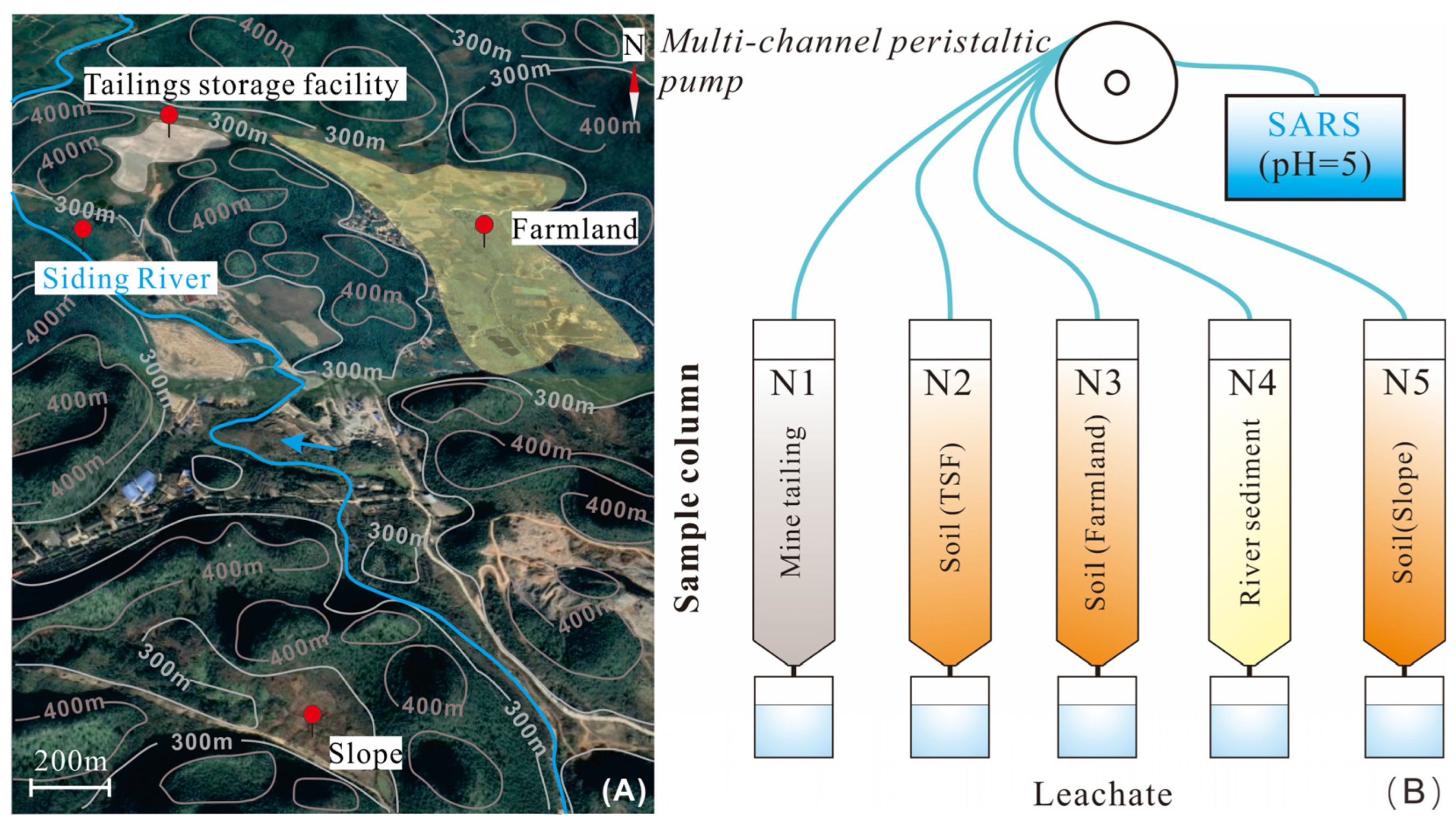
2.1. Study Area and Sample Collection

The Siding Lead–Zinc Mine is located in Siding Town, Liuzhou City, northern Guangxi Zhuang Autonomous Region, with geographic coordinates of 109°31′~109°33′ E and 25°24′~25°34′ N. The mining area is characterized by karst topography, featuring well-developed limestone peak clusters and a river system, with the Siding River as the main watercourse. The dominant soil type is red soil, derived from parent materials such as limestone, sandy shale, and dolomite. The Siding Lead–Zinc Mine lies within the Xiang-Gui Lead–Zinc Metallogenic Belt along the southern margin of the Yangtze Platform [25]. The stratigraphic lithology of the mining area primarily consists of dolomite, sandstone, and limestone. The main metallic minerals include sphalerite (ZnS), galena (PbS), and pyrite (FeS₂), with trace amounts of chalcopyrite (CuFeS₂), bornite (Cu₅FeS₄), and tetrahedrite (Cu₁₂Sb₄S₁₃).

This study targeted tailings, soils, and river sediments from the Siding Lead–Zinc Mine. Specific sampling locations are shown in Figure 1A. The tailings from the Siding Lead–Zinc Mine are classified as carbonate-type tailings [26]. However, due to their high dolomite content, they can also be categorized as dolomite-type tailings [27]. The soil in the mining area is typical red soil of the karst region, consisting of weakly alkaline red clay formed through decalcification weathering of parent rocks. Soil samples were collected from three distinct regions: soil surrounding the tailings storage facilities (TSFs), farmland soil, and slope soil. A river sediment sample was collected from the Siding River. Sampling was conducted using the five-point sampling method at a depth of 0~20 cm. After collection, visible impurities such as leaves and stones were removed. Each sample was assigned a unique identifier, labeled with location information, and properly sealed. Samples were air-dried at room temperature. All sampling and processing procedures strictly followed the Technical Specifications for Soil Environmental Monitoring (HJ/T 166−2004) [28]. Polished thin sections were prepared at the Guilin University of Technology for subsequent mineralogical analysis.

2.2. Experimental Methods

2.2.1. Preparation of Simulated Acid Rain Solution (SARS)

The preparation of a simulated acid rain solution was primarily based on the pH and major chemical constituents of natural rainfall. To enhance the leaching effect of acid rain in this study, the composition of acid rain was modeled based on rainfall data from Liuzhou City. In this experiment, the molar ratio of SO₄²⁻ to NO₃⁻ in the leaching solution was set to 3:1, with a pH of 5.0. The simulated acid rain solution was prepared by diluting a mixture of sulfuric acid (H₂SO₄, analytical reagent grade) and nitric acid (HNO₃, analytical reagent grade) with deionized water.

2.2.2. Column Leaching Test

The experimental apparatus configuration is shown in Figure 1B.

The column leaching setup consisted of five acrylic columns (inner diameter: 10 cm; height: 100 cm) with sealed top and bottom caps, labeled N1 to N5. The lower end of the glass column was designed in a funnel shape to facilitate efficient collection of the leachate. A silicone tube was inserted into the upper cover and connected to both a peristaltic pump and an acid solution reservoir. The acid solution was delivered into the glass column via the peristaltic pump. To enhance the effect of acid leaching on the release of heavy metals and ensure sufficient interaction between the leachate and the soil, an intermittent leaching method was employed. The leaching experiment was carried out using a multi-channel variable-speed peristaltic pump (BT100S, Leadfluid, Baoding, China). Column N1 contained tailings, N2 contained soil from the area surrounding the tailings pond, N3 contained agricultural soil, N4 contained riverbed sediment from the Siding River, and N5 contained slope soil from an area remote from the tailings pond. All samples were air-dried indoors and sieved through a five-mesh screen (4.00 mm aperture) before being packed into the columns at a height of approximately 90 cm. The packing mass was approximately 18 kg for tailings (N1) and about 9 kg for the soil and sediment samples (N2–N5). Under room temperature conditions, each column was leached for 12 h per day over a period of 57 consecutive days, at a flow rate of 2.2 mL·min⁻¹. Leachate was collected every 3 days, resulting in a total of 19 sampling events. All experimental procedures and soil sample pretreatment strictly followed the standard protocol “Column Leaching Test for Chemicals in Soil” (GB/T 41667−2022) [29].

2.2.3. Analytical Methods

The pH values of the soil, tailings, and sediment samples were determined according to the national standard HJ 962−2018 [30], while the pH value of leachates from column experiments was measured following the national standard HJ 1147−2020 [31]. The total dissolved solid (TDS) value was determined using the conductivity method, in accordance with the national standard HJ 506-2009 [32]. Backscattered electron (BSE) images of sample thin sample sections were captured using an electron probe microanalyzer (EPMA, JXA-8230, JEOL Ltd., Tokyo, Japan). The modal abundances of individual minerals were calculated using the grid-counting method in conjunction with the Adobe Photoshop 2023 (Adobe Inc., San Jose, CA, USA). Mineral phase analysis was conducted using an X-ray diffractometer (XRD, X’Pert PRO, PANalytical B.V., Almelo, The Netherlands. The speciation of heavy metals in soil was analyzed using an improved three-step sequential extraction procedure proposed by the Community Bureau of Reference (BCR) of the European Commission [33], categorizing the metals into an acid-soluble fraction (F1), reducible fraction (F2), oxidizable fraction (F3), and residual fraction (F4). The samples (0.10 g) were digested with a mixture of HNO₃, HClO₄, HF, and HCl using a four-acid digestion method on a hot plate. The concentrations of As, Cd, Cr, Cu, Pb, and Zn were determined using inductively coupled plasma mass spectrometry (ICP-MS, Agilent 7500, Agilent Technologies Inc., Santa Clara, CA, USA), following the national standard HJ 700-2014 [34]. Prior to analysis, the ICP-MS instrument was calibrated using a tuning solution and the relative standard deviation (RSD) of the signal intensity for the elements in the test solution was required to be ≤5% to ensure data stability and reliability. To guarantee analytical precision, accuracy, and data quality, blank samples, 20% parallel samples, and a certified reference soil sample (GBW 07449) were simultaneously analyzed. The results for the blank samples were below the detection limit; the relative deviation of the parallel samples was within ±25%; and the spiked recovery rate of the standard sample ranged between 90% and 99%. All laboratory vessels used in the analysis were pre-soaked in dilute acid overnight, ensuring the reliability and credibility of the analytical results.

2.3. The Cumulative Release of Heavy Metals

The cumulative release of heavy metals is a key parameter for evaluating the migration and release potential of heavy metals in environmental samples. This release can be quantified from two perspectives: by element and by testing time. The element-based dimension is the cumulative release mass of heavy metal i over the entire leaching period, which is denoted as m_i. The time-based dimension is the total release mass of all heavy metals at the j-th testing event, which is denoted as m_j. The formulas are expressed as follows:

$$m_i={\displaystyle \sum _{i=1}^n\left(\frac{C_{ij}\times v_j}{1000}\right)}$$

(1)

$$m_j={\displaystyle \sum _{i=1}^l\left(\frac{C_{ij}\times v_j}{1000}\right)}$$

(2)

where m_i is the cumulative release mass of heavy metal i (mg), representing the total amount of element i released into the leachate throughout the entire experiment; m_j is the total release mass of all heavy metals (mg) at the j-th testing event; C_ij is the concentration of heavy metal i in the leachate at the j-th testing event (μg·L⁻¹); V_j is the volume of leachate collected at the j-th sampling event (L); n is the total number of testing events; and l is the total number of heavy metal species analyzed.

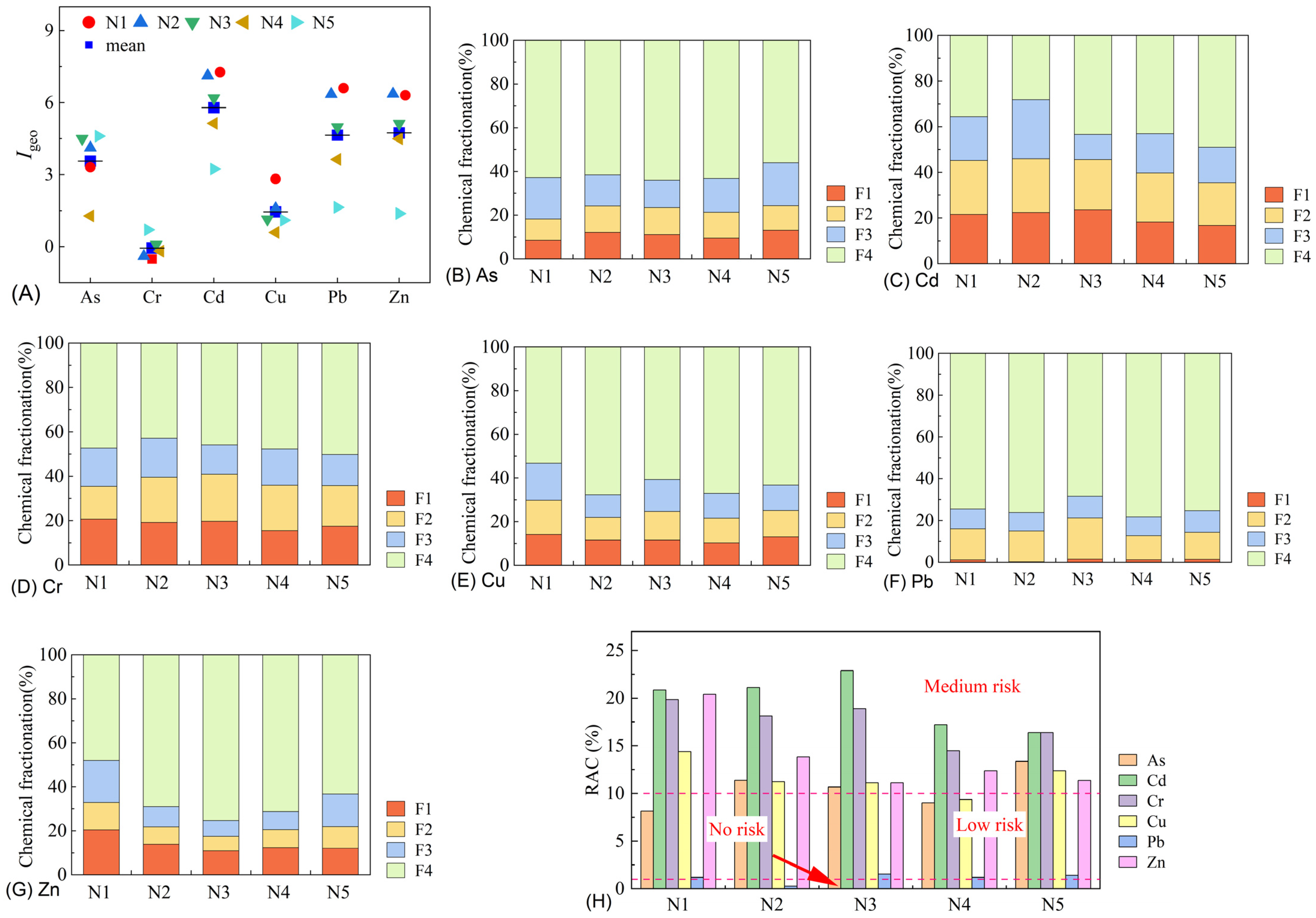
2.4. Environmental Risk Assessment

The extent of heavy metal pollution in the samples was assessed using the geoaccumulation index (I_geo). The calculation formula is as follows:

$$I_{\mathrm{geo}}={\log }_2{\displaystyle \frac{C_i}{k\times B_{\mathrm{i}}}}$$

(3)

where I_geo represents the geoaccumulation index; C_i is the measured concentration of heavy metal i in the soil; B_i is the geochemical background concentration of heavy metal i in the soil, expressed in mg·kg⁻¹; and k is the correction factor, typically set to 1.5. The average concentrations of heavy metals in the soils of Liuzhou (Pb: 38.1 mg·kg⁻¹, Zn: 129 mg·kg⁻¹, and Cd: 0.73 mg·kg⁻¹) were used as background reference values. The I_geo value is divided into seven classes: I_geo ≤ 0, uncontaminated; 0 < I_geo ≤ 1, unpolluted to moderate; 1 < I_geo ≤ 2, moderately polluted; 2 < I_geo ≤ 3, moderate to strong; 3 < I_geo ≤ 4, strongly polluted; 4 < I_geo ≤ 5, very strongly polluted; and I_geo ˃ 5, extremely polluted [35].

The Risk Assessment Code (RAC), originally proposed by Perin in 1985 [36], is commonly used to evaluate the mobility and bioavailability of heavy metals in soils. This method quantifies the potential ecological risk posed by heavy metal contamination and converts pollution levels into actionable risk categories or indices. The RAC value is calculated based on the proportion of exchangeable metal fractions in the soil [37]. The migration risk of heavy metals in the samples was assessed using the percentage of acid-extractable fraction (F1) of heavy metals relative to the total content, known as the risk assessment code (RAC) value [38]. The RAC value is divided into five classes: RAC < 1%, no risk; 1% ≤ RAC < 10%, low risk; 11% ≤ RAC < 30%, medium risk; 31% ≤ RAC < 50%, high risk; and RAC ≥ 50%, very high risk.

The Water Quality Index (WQI) was used to assess the changes in water quality caused by heavy metal leaching in the column experiment samples. The calculation formula is as follows:

$$\mathrm{WQI}={\displaystyle \sum \left({\mathrm{W}}_i\times \frac{C_i}{S_{\mathrm{i}}}\right)}\times 100$$

(4)

$${\mathrm{W}}_i={\displaystyle \frac{{\mathrm{w}}_i}{{\displaystyle \sum {\mathrm{w}}_i}}}$$

(5)

where WQI represents the Water Quality Index; C_i is the measured concentration of heavy metal i in the water, S_i is the threshold value of heavy metal i as specified in the Chinese drinking water quality standard GB 5749–2022 [39], expressed in mg·kg⁻¹; and w_i is the weight factor for heavy metal i in drinking water [40]. The corresponding values for As, Cd, Cr, Cu, Pb, and Zn are 5, 5, 5, 2, 5, and 1, respectively. The WQI values are divided into five classes: WQI < 50, excellent; 50 ≤ WQI < 100, good; 100 ≤ WQI < 200, poor; 200 ≤ WQI < 300, very poor; and WQI ≥ 300, undrinkable.

2.5. Machine Learning Methods

All experimental data (n = 95) were divided into a training set (n = 67) and a test set (n = 28). The Random Forest (RF) and Support Vector Machine (SVM) models were developed in the Spyder environment of the Anaconda Navigator platform. In machine learning modeling, hyperparameter tuning plays a critical role in determining model performance. Different combinations of hyperparameters can significantly affect the model’s performance metrics—such as generalization ability, accuracy, and robustness—as well as computational efficiency, including training time [41]. For SVM model key hyperparameters—such as kernel parameters and the penalty parameter—substantially influence model complexity and predictive performance. Commonly used kernel functions include the linear kernel, polynomial kernel (Poly), and radial basis function (RBF) kernel [42]. For the Random Forest (RF) algorithm, important hyperparameters include the number of trees, splitting criteria and nodes, the number of randomly selected variables, and the minimum number of samples required to split a node [43]. To reduce the risk of model overfitting and enhance generalization capability, this study employed grid search with cross-validation (GridSearchCV) to systematically evaluate a predefined set of parameter combinations [44]. This method exhaustively searches the parameter space and uses cross-validation to assess model performance, thereby identifying the optimal hyperparameter configuration. Cross-validation itself is a crucial technique for evaluating predictive models. Among different cross-validation strategies, five-fold cross-validation offers a good trade-off between evaluation reliability, model stability, and computational efficiency, providing more dependable results than three-fold cross-validation while being less computationally demanding than ten-fold cross-validation [45]. Through the testing and comparison of multiple parameter combinations, the optimal model structures and parameter configurations were finally determined.

2.6. Statistical Analyses

All statistical analyses were performed using SPSS 22.0 (IBM Corp., Armonk, NY, USA), WPS Office (Kingsoft Corp., Beijing, China), and OriginPro 2023 (OriginLab Corp., Northampton, MA, USA). Statistical significance was determined using SPSS 22.0, with a threshold of p < 0.05. Graphical illustrations and data visualization were carried out using OriginPro 2023 and WPS Office.

3. Results and Discussion

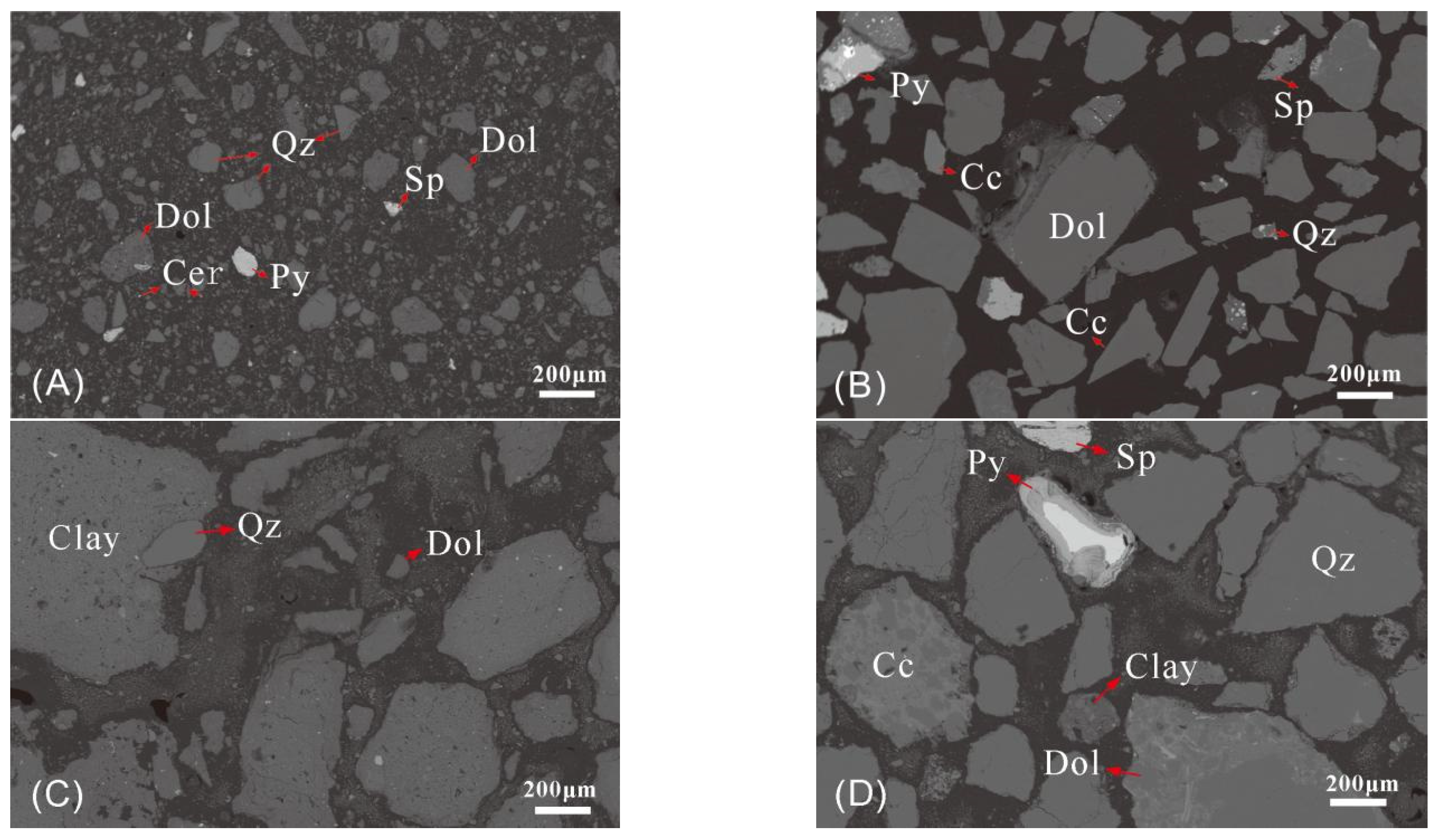
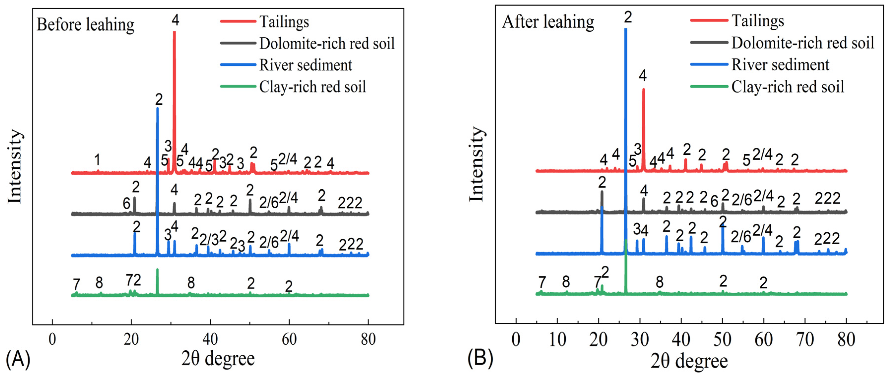
3.1. Mineralogical Characteristics of the Samples

The mineral compositions of the samples were relatively simple, with the primary minerals including dolomite, quartz, calcite, clay minerals, pyrite, and sphalerite (

Table 1. Mineral phase abundances of the samples (%).

Sample		N1 *	N2	N3	N4	N5
Dolomite	Dol	50	70	68	18	5
Calcite	Cc	0	12	9	3	<1
Quartz	Qz	38	8	11	71	0
Clay minerals	Clay	0	1	9	0	93
Pyrite	Sp	8	5	2	5	<1
Cerussite	Cer	1	1	0	0	0
Sphalerite	Py	3	3	1	3	0

* N1, tailings; N2, soil surrounding the TSF; N3, farmland soil; N4, river sediment; N5, slope soil (hereinafter the same).

; Figure 2).

Electron probe microanalysis revealed that, except for N5, the samples were predominantly composed of carbonate minerals. Tailings (N1, Figure 2A) contained up to 12% unsorted metallic minerals, such as sphalerite, cerussite, and pyrite. Dolomite and calcite were abundant in N2 and N3 (Figure 2B), with N2 exhibiting a higher content of sulfide minerals than N3. The primary minerals in N4 (Figure 2C) were quartz and dolomite, accompanied by minor clay minerals; its metallic mineral content ranked second only to the soil surrounding the tailings pond. In contrast, N5 (Figure 2D) mainly consisted of coarse-grained clay minerals, with minor amounts of dolomite and quartz.

Further mineral phase analysis using XRD (Figure 3A) indicated that the clay minerals were dominated by magnesium- and aluminum-rich layer silicates, such as chlorite, montmorillonite, and kaolinite. Ca(Zn, Mg)(CO₃)₂ solid solutions commonly occur in the oxidation zones of lead–zinc deposits. Previous studies [46] have demonstrated that Zn dolomite forms through the reaction between metal-laden, oxygen-rich atmospheric precipitation and pre-existing dolomite that hosts zinc sulfide minerals and has undergone intense weathering. The replacement of the original dolomite by supergene Zn dolomite is a gradual process [47], typically proceeding through the following stages: progressive zinc enrichment of dolomite crystals (“zinc mineralization”) →partial dedolomitization →complete replacement of dolomite by smithsonite. A certain amount of CaSO₄·2H₂O was also identified in the tailings, representing a common secondary mineral in the oxidation zone of sulfide tailings. However, gypsum was not detected via electron probe analysis, likely due to its low content or fine particle size. Gypsum plays a significant role as a heavy metal sorbent in both acidic and neutral mine drainage environments [48]. However, during short-term rainfall events, soluble metal sulfate minerals such as gypsum may dissolve, potentially leading to the rapid release of substantial amounts of heavy metals into the environment [49].

Combined EPMA and XRD analyses further indicated that the mineral composition of the samples remained largely unchanged after acid leaching (Figure 3B). However, acid leaching led to a reduction in the contents of calcite, cerussite, sphalerite, pyrite, and gypsum, suggesting that acid rain had limited effects on the crystal structure of most minerals. Although both dolomite and calcite are carbonate minerals, dolomite has a more stable crystal structure and stronger acid resistance, leading to a faster dissolution rate of calcite under acidic conditions. Pyrite (FeS₂) typically remains unreactive under mildly acidic conditions, but a slight decrease in its XRD peak intensity was observed after acid leaching. Previous studies [50] have demonstrated that when pyrite, calcite, and dolomite undergo simultaneous oxidation, Ca(OH)₂ and Mg(OH)₂ precipitates may form on the pyrite surface, thereby reducing the intensity of its diffraction peaks. Gypsum, being a soluble mineral, tends to dissolve readily into leachate under continuous acid leaching.

3.2. Heavy Metal Contamination Characteristics of the Samples

The concentrations, chemical fractions, and mobility risks of heavy metals in the samples are presented in

Table 2. Physicochemical parameters such as pH, water content, and total heavy metals before leaching (mg·kg⁻¹).

Sample	Location	Type	pH	ω (%)	As	Cd	Cr	Cu	Pb	Zn
N1	TSK	Tailings	7.24	14.7	321 ± 3.42	169 ± 5.35	117 ± 3.9	265 ± 8.42	5562 ± 145	15362 ± 787
N2	TSK	Red soil	7.07	18.6	563 ± 5.75	153 ± 2.46	127 ± 4.78	113 ± 2.73	4677 ± 150	16001 ± 429
N3	Farmland	Red soil	7.33	13.6	731 ± 12.5	79.9 ± 1.58	178 ± 6.95	82.8 ± 0.22	1808 ± 23.5	6786 ± 376
N4	Siding River	Sediment	7.82	14.7	78.7 ± 0.47	38.5 ± 0.47	147 ± 1.77	56.5 ± 1.25	711 ± 5.51	4389 ± 215
N5	Slope	Red soil	7.37	21.4	786 ± 10.6	10.3 ± 0.57	272 ± 3.27	80.5 ± 2.71	178 ± 5.38	506 ± 30.5
Average value			7.37	16.6	496 ± 3.54	90.1 ± 1.23	168 ± 2.01	120 ± 1.87	2587 ± 42.1	8609 ± 199
Liuzhou [31]					21.6	0.73	111	25.0	38.1	129
China [32]					11	0.1	61	23	26	74
Risk screening value					60	65	5.7	18000	800

and Figure 4A. The concentrations of heavy metals varied considerably among different sample types; however, all samples exhibited significantly higher heavy metal contents than the background values for both Liuzhou and the national average in China [51]. Among the metals analyzed, Cr and Cu showed relatively low levels of contamination, with mean geoaccumulation index (I_geo) values of 0 and 1.5, respectively. In contrast, the concentrations of As, Cd, Pb, and Zn exceeded the soil pollution risk screening values for land designated for construction, with corresponding average I_geo values of 3.6, 5.8, 4.6, and 4.7, indicating moderate to severe contamination levels.

The tailings sample exhibited the highest concentrations of Cd, Pb, and Zn among all samples. The slope soil showed the lowest concentrations of heavy metals, except for As. Notably, the As concentration in the slope soil was relatively high, with an I_geo value of 4.6, indicating heavy contamination (Figure 1A). This may be attributed to the high content of clay minerals in the slope soil. Clay minerals generally possess negatively charged surfaces and thus exhibit a certain degree of adsorption capacity for heavy metals. However, fluctuating redox conditions can enhance the bioavailability of heavy metals in the environment [52]. In contrast, the soil collected near the tailings pond contained 15, 26, and 32 times higher concentrations of Cd, Pb, and Zn, respectively, compared with the slope soil, with I_geo values exceeding 6—indicating severe contamination and suggesting that leakage from the tailings facility may have contributed to the pollution of surrounding soils.

As shown in Figure 4B–G, the residual fraction dominated the chemical forms of heavy metals, with the average proportions ranked as follows: Pb (74.3%) > Zn (65.2%) > Cu (60.1%) > As (59.4%) > Cr (44.4%) > Cd (38.4%). The mobility risk of heavy metals in the samples is illustrated in Figure 4H. Pb exhibited minimal mobility risk, with an average RAC value of 1%. In contrast, Cd showed the highest mobility risk, with a mean RAC value of 20%. According to Lim [53] and Luo [54], the high Ca²⁺ content in soils competes with Cd²⁺ for uptake sites at plant root surfaces, making Cd more mobile. Therefore, Cd poses a higher mobility risk in dolomite-rich soil compared with other soil types.

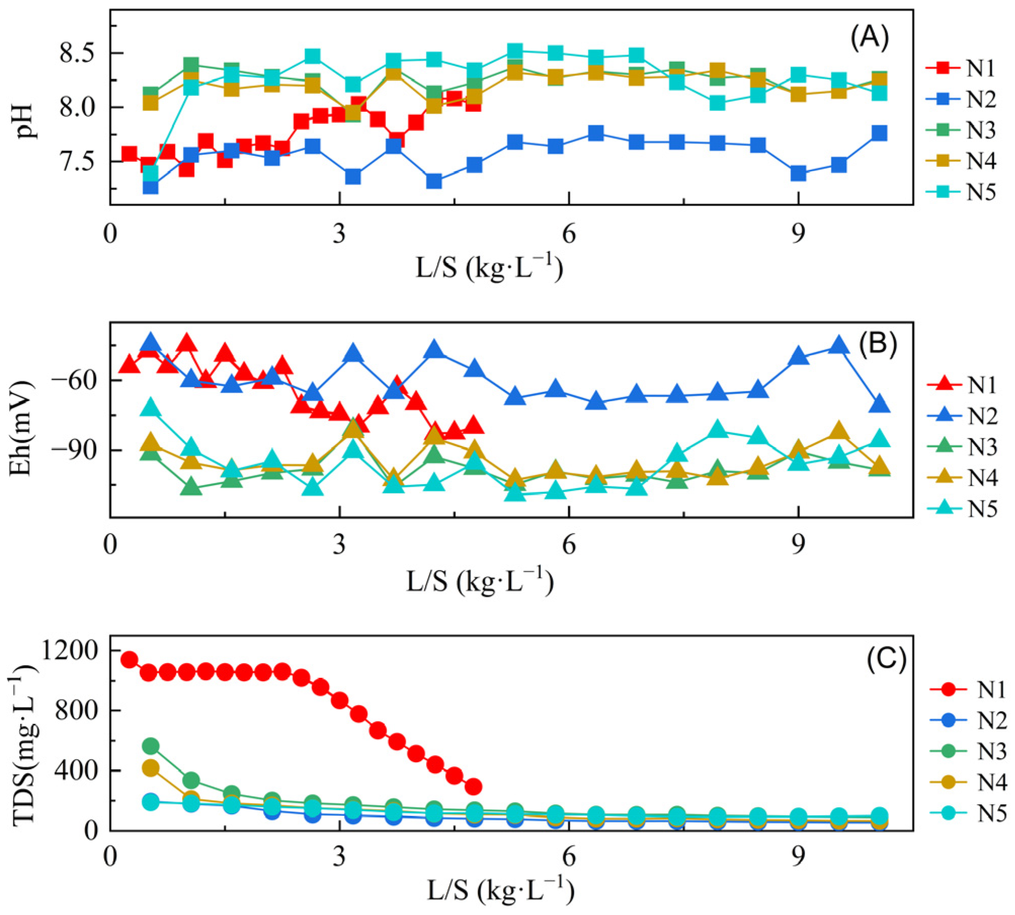
3.3. The pH, Eh, and TDS Characteristics of Sample Leachates

The liquid-to-solid (L/S) ratio is an important parameter for evaluating the heavy metal release potential of different samples [55]. The L/S ratio helps eliminate the influence of sample type, leaching volume, and experimental setup, thereby allowing for a meaningful comparison of heavy metal release capacity among samples. Due to the higher bulk density of tailings compared with soil and river sediment, their L/S ratios are lower under the same experimental conditions. The variations in pH and Eh of leachates from different soil columns are illustrated in Figure 5.

The average pH and Eh values of the leachate from each soil column were 7.97 and −76.7 mV, respectively. These results suggest that the soil samples from the mining area exhibit a strong neutralizing capacity toward the simulated acid solution. In addition, the negative Eh value indicates that the leachate is under mildly reducing conditions. The average pH and Eh values of the leachates from N1 and N2 were higher than those from N3 to N5. The oxidation of sulfide minerals releases acidic ions [56], resulting in sulfate-rich acidic effluents, which can lower the pH and increase the Eh of the leachate. However, the dissolution of carbonate minerals can neutralize H⁺ ions, thereby raising the pH of the leachate [57]. Consequently, samples with higher contents of metal-bearing minerals (N1 and N2) tended to exhibit lower pH and higher Eh values, although this trend was moderated by the acid-buffering effect of carbonates. Additionally, the prolonged water-saturated conditions of the samples reduced oxygen diffusion, fostering an anaerobic environment that also contributed to the reducing nature of the leachates [58].

The total dissolved solid (TDS) concentration in the leachate from N1 was significantly higher than that of the other samples. During the early stages of the experiment, N1 exhibited a plateau phase with a mean TDS value of 1061 mg·L⁻¹, followed by a gradual decline. In contrast, the TDS levels in samples N2 through N5 decreased steadily throughout the experiment with relatively stable variation. According to Skousen et al. [59], the primary ionic components of neutral mine drainage include Ca²⁺, K⁺, Mg²⁺, Na⁺, SO₄²⁻, and HCO₃⁻, and the dissolution of sulfide minerals can also result in TDS concentrations exceeding 1000 mg·L⁻¹. Therefore, the high concentration of soluble salts in the leachate from N1 under acid leaching conditions is likely attributable to its elevated contents of carbonate and sulfide minerals.

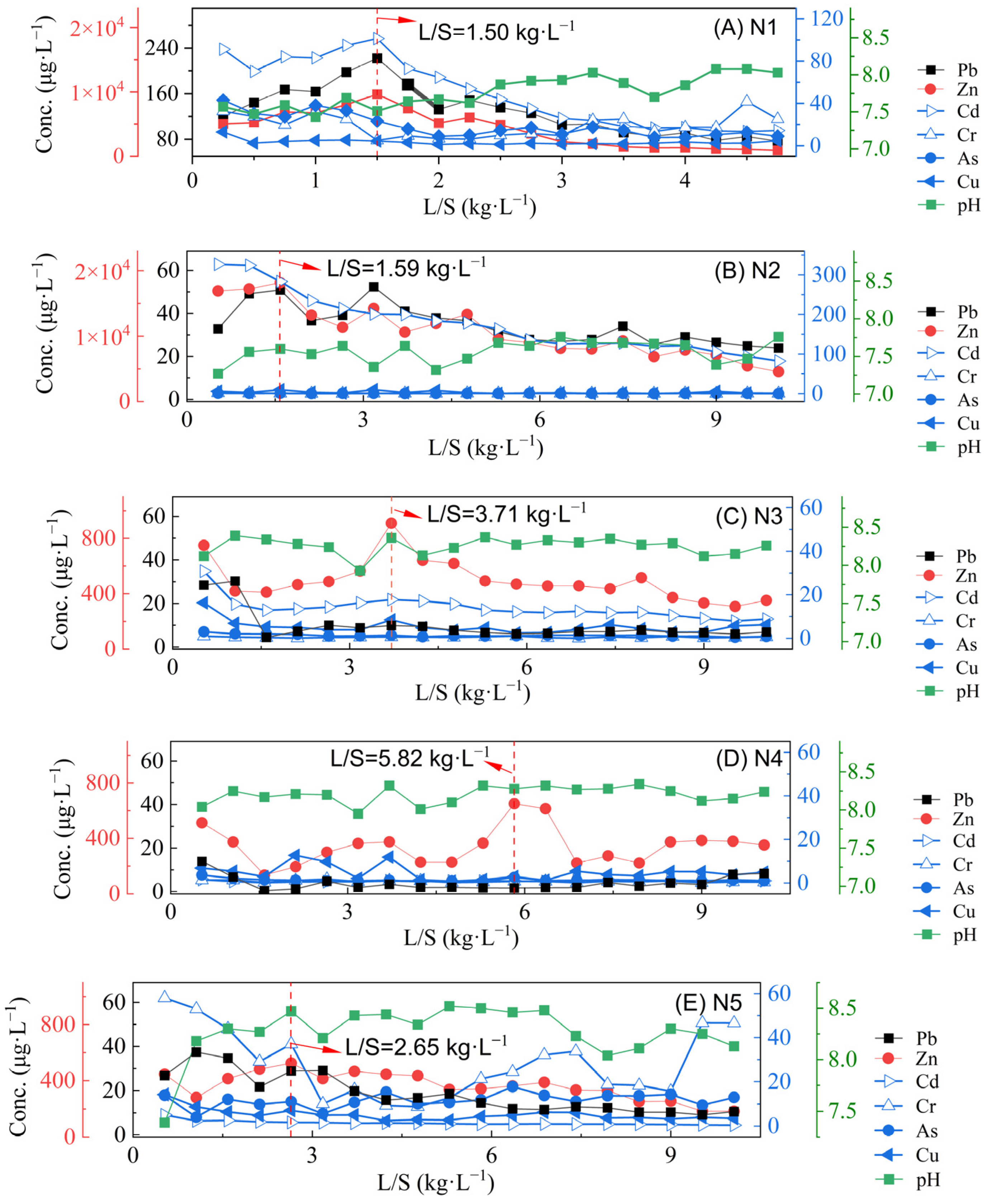
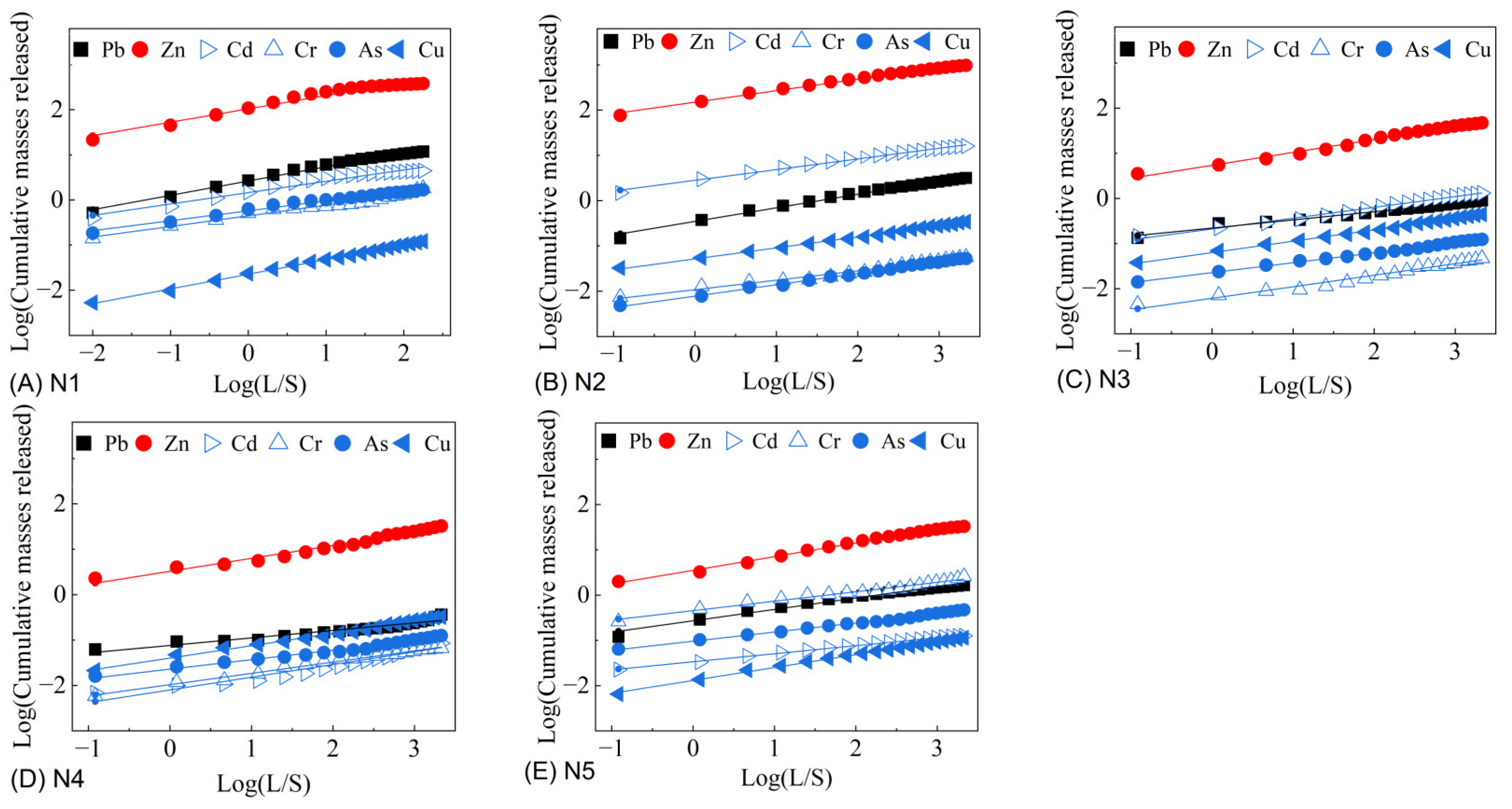
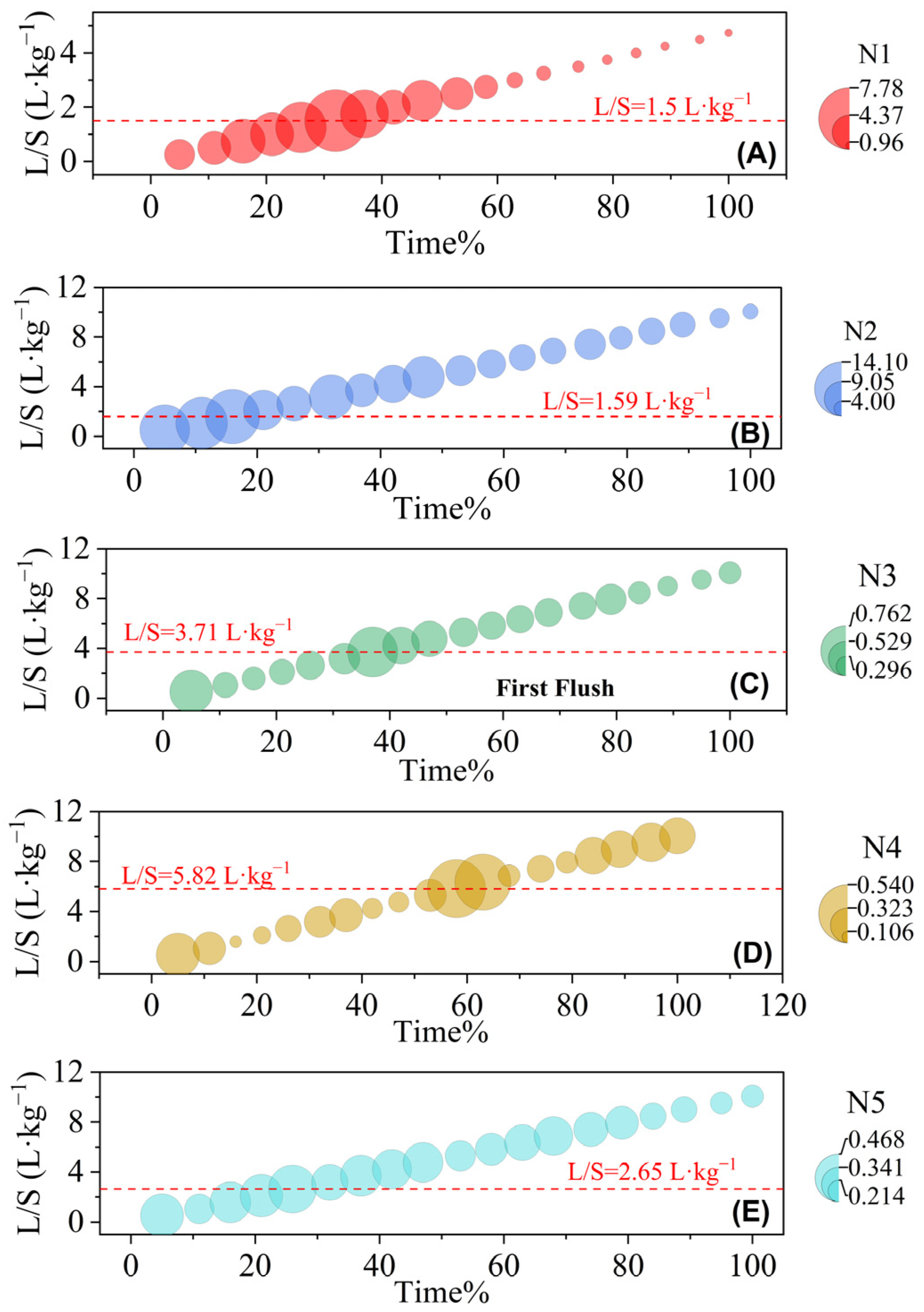
3.4. Heavy Metal Concentrations and Cumulative Release Characteristics in Leachates

The concentrations and cumulative release of heavy metals in the leachates from different samples are shown in Figure 6, Figure 7 and Figure 8. The average concentrations of heavy metals in the leachates (μg·L⁻¹) were as follows: Zn (3218) > Cd (48.3) > Pb (39.1) > Cr (9.81) > Cu (5.69) > As (5.39). Correspondingly, the average cumulative release amounts (mg·kg⁻¹) were as follows: Zn (1465) > Cd (21.9) > Pb (17.9) > Cr (4.52) > Cu (2.63) > As (2.45).

The release of heavy metals was dominated by Zn, followed by Cd and Pb. Compared with the screening values for Class III groundwater quality standards (GB/T 14848-2017) [60], the concentrations of Cd and Zn in the leachates were significantly above the thresholds—on average, 10 and 3 times higher, respectively. Among the different samples, only N4 showed no exceedance of heavy metal standards in its leachate. The other samples exhibited varying degrees of heavy metal exceedance: As, Cd, Pb, and Zn in N1; Cd and Zn in N2; Cd in N3; and As in N5.

The total mass of heavy metals released from different samples and its relationship with the L/S ratio and time are shown in Figure 8. As the liquid-to-solid (L/S) ratio increased, the heavy metal concentrations in the leachates generally exhibited a trend of initial increase followed by a gradual decrease. During the initial stage of the simulated soil column experiment, the addition of acid caused the rapid dissolution and release of soluble heavy metal salts accumulated on the surface of the dry samples. Previous studies [61] have often attributed this rapid change in heavy metal concentrations in the leachate to an initial flushing effect. The intensity and composition of this flushing are influenced by factors such as rainfall intensity, preceding drought duration, soil surface type, and local human activities. Notably, longer drought periods typically result in higher pollutant loads [62], which dissolve quickly and release metals when leaching begins. Once the L/S ratio reaches a certain threshold, heavy metal release peaks and then tends to stabilize as the leaching of the “parent” heavy metal pool progresses at a slower rate [63].

In this study, for heavily contaminated samples such as N1 and N2, the initial flush effect induced by acid leaching was pronounced, with heavy metal release dominated by Cd, Pb, and Zn. The peak L/S ratios for these samples were 1.5 L·kg⁻¹ (N1) and 1.59 L·kg⁻¹ (N2), respectively. At this stage, the elution time for the N1 sample accounts for only 32% of the total experimental duration, yet its cumulative heavy metal release reaches approximately 50% of the total release. Similarly, the elution time for the N2 sample represents just 16% of the total period, while its cumulative heavy metal release is about 25% of the total. In contrast, samples with lower heavy metal contamination, such as N3 through N5, exhibit a weaker initial flushing effect. For these samples, the heavy metal release is predominantly zinc and the L/S values corresponding to their peak releases are higher than those of N1 and N2, following the order N4 (5.82) > N3 (3.71) > N5 (2.65).

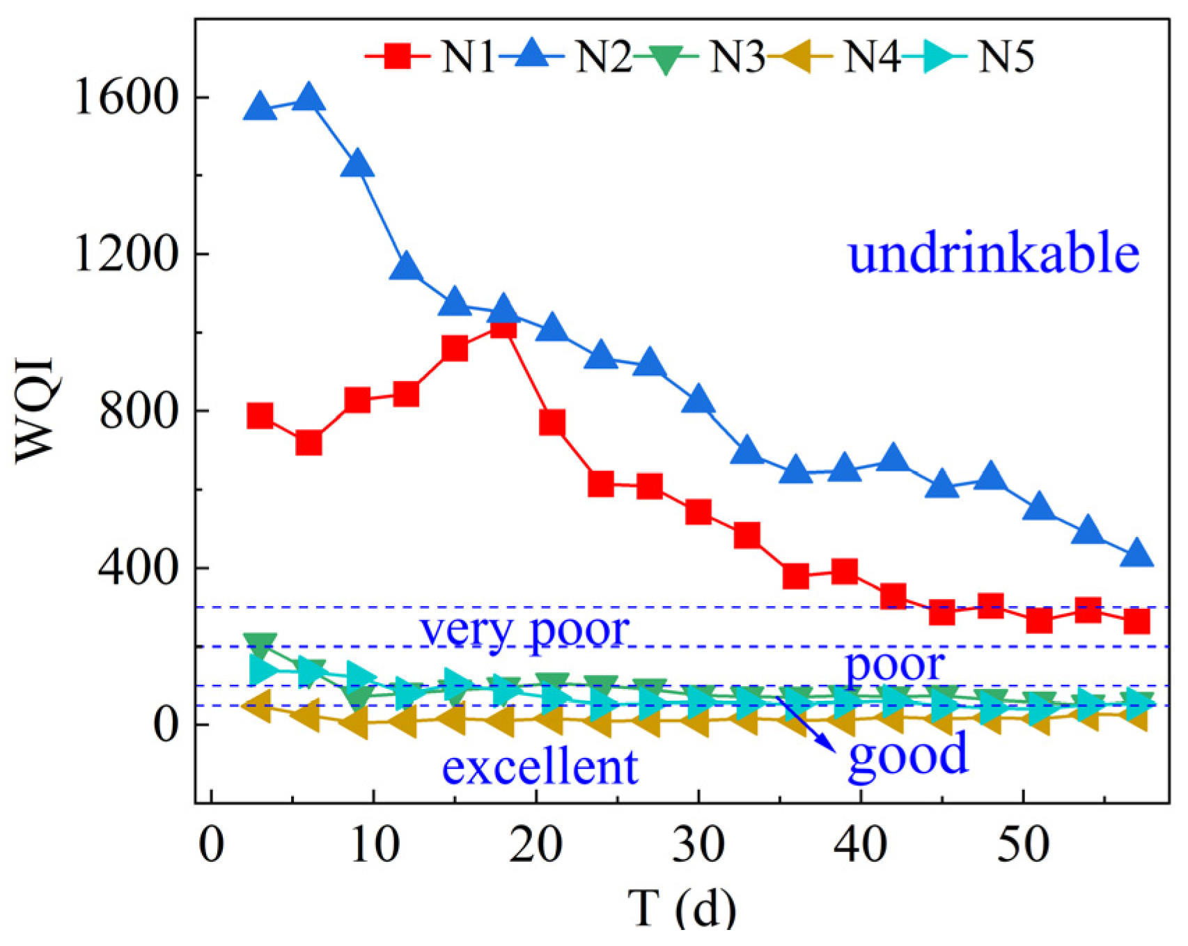
3.5. Environmental Impact Assessment of Leachates

The Water Quality Index (WQI) values of leachates from different samples are shown in Figure 9. As leaching progressed, the WQI values generally exhibited a decreasing trend, indicating an overall improvement in leachate water quality over time. The WQI values ranged from 0 to 1592, with an average of 325, corresponding to a classification of “non-potable”.

Significant variations in water quality grades were observed among different leachates. The leachate from river sediment displayed the best water quality, consistently classified as “excellent,” with an average WQI value of 17. In contrast, leachates from tailings and soils near the tailings pond exhibited the highest water quality, mostly falling within the “non-potable” category. Among all samples, the leachate from the soil surrounding the TSF had the worst quality, with an average WQI value 52 times higher than that of river sediment. Similarly, the average WQI of leachate from the tailings sample was 33 times that of the river sediment. These results suggest that during the initial stages of acid deposition, acid rain accelerates the release of heavy metals from the soil, leading to a deterioration in water quality in the mining area. However, as rainfall continues and the leaching process progresses, the concentrations of heavy metals in the leachate decrease, resulting in a gradual improvement in water quality. Through understanding the temporal variation characteristics of the Water Quality Index (WQI) in water bodies, identifying the critical periods of heavy metal pollution in mining areas, and enhancing the stability of tailings ponds or improving the isolation and treatment of mine drainage during the rainy season, the pollution load resulting from the migration and release of heavy metals can be effectively mitigated.

3.6. Correlation Analysis and Machine Learning-Based Prediction of Heavy Metal Migration

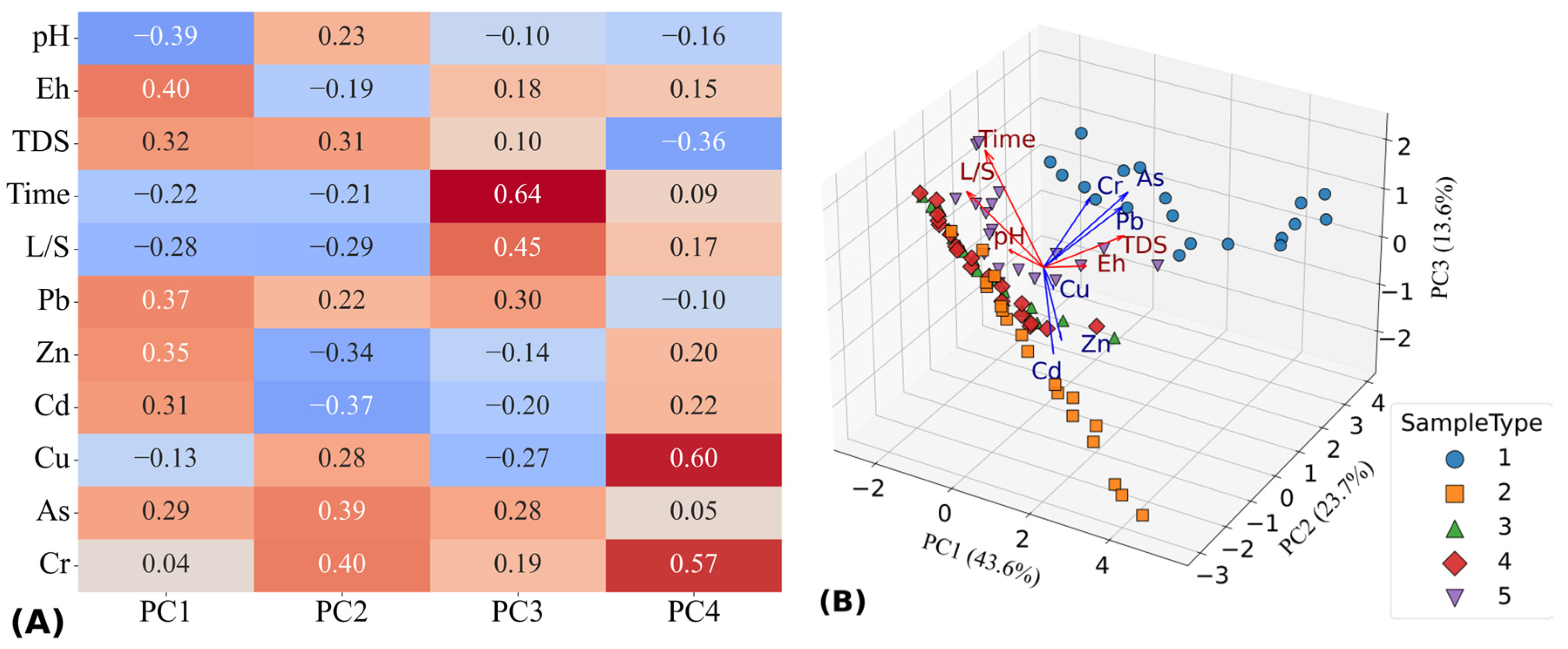
3.6.1. Correlation Analysis

Principal component analysis is a commonly used statistical method that maximally explains the variance among all variables [64], while reducing the dimensionality of the data and retaining most of its important information. PCA was employed to classify the experimental data in order to analyze the characteristics of heavy metal release in mining areas, including environmental variables (TDS, Eh, pH, L/S, and time) and heavy metals (As, Cd, Cr, Cu, Pb, and Zn). The results are shown in Figure 10.

The results of the principal component analysis (PCA) demonstrated that each environmental factor exerted a significant driving influence on the release of heavy metals during the leaching process. The contribution rates of PC1, PC2, and PC3 were 43.6%, 23.7%, and 13.6%, respectively, cumulatively explaining approximately 80.9% of the total variance in the original dataset. This indicates a strong dimensionality reduction effect, with the three-dimensional principal component plot effectively capturing the characteristics of the original data. The distribution of different sample types within the principal component space exhibited clear separation, reflecting distinct spatial migration trends in heavy metal release behavior.

Specifically, sample N1 was primarily located in the positive directions of PC2 and PC3, strongly influenced by Eh and TDS, suggesting that tailings have a high potential for heavy metal release under oxidizing conditions. Sample N2 was concentrated in the positive direction of PC1 and was significantly affected by the L/S ratio and leaching time, with a release trend that increased as the leaching progressed. In contrast, samples N3 and N4 were mainly distributed in the negative direction of PC1, indicating that heavy metal release from agricultural soil and river sediment was more influenced by acidic conditions, with Zn and Cd showing particularly active release behavior. Sample N5 was positioned near the origin of the principal component space, indicating a generally low release capacity of heavy metals.

According to the PCA loading results, PC1 was primarily composed of Eh (+0.40), Pb (+0.37), Zn (+0.35), and Cd (+0.31), with pH exhibiting a negative loading (−0.39), suggesting that redox conditions and pH are the key controlling factors for this component. A decrease in Eh and an increase in pH were associated with enhanced heavy metal release. PC2 showed high loadings for Cr (+0.40), As (+0.39), and TDS (+0.31), while Cd and Zn were negatively correlated, indicating that this component may represent the influence of mineral solubility on migration behavior. However, Zn and Cd may undergo precipitation or complexation during this process. In PC3, leaching time (+0.64) and L/S ratio (+0.45) exhibited strong loadings, representing typical process-controlling variables, and indicating that heavy metal release intensity increased with time and liquid–solid ratio. In PC4, high loadings of Cu (+0.60) and Cr (+0.57) suggested potential re-release processes in the later leaching stages, possibly due to desorption or changes in metal speciation.

As, Cd, Pb, and Zn consist of chalcophile elements with similar geochemical behavior, indicating that their migration and release may be governed by similar geochemical mechanisms, such as acid dissolution and co-precipitation processes [65]. Cd, Pb, and Zn are the primary pollutants in the mining area; Cd and Zn are weakly adsorbed and highly water-soluble [66], and Cd is often isomorphously substituted in Zn-bearing minerals. In contrast, Pb is strongly adsorbed and poorly soluble, exhibiting lower mobility [67]. The correlation analysis shows that the release of Cd, Pb, and Zn is positively correlated with Eh and negatively correlated with pH. In the weathered zone of carbonate-hosted Pb–Zn deposits, Cd²⁺, Pb²⁺, and Zn²⁺ often occur in sulfate and carbonate forms [68], but PbSO₄ exhibits relatively poor acid solubility. In the early stage of the experiment, sulfuric acid rock solution (SARS) dominated the leaching environment and acid-soluble heavy metals were released first [2], such as Cd- and Zn-bearing sulfates and carbonates, as well as Pb carbonates. Moreover, the presence of sulfate minerals can further accelerate the dissolution of carbonate minerals [69].

The release of Pb in N1 was higher than in the other samples and the release rate increased with the L/S ratio during the early stage, which is likely related to the high content of Pb-bearing carbonate minerals in this sample. In the later stages of the experiment, the leachate became increasingly alkaline, with OH⁻ and SO₄²⁻ gradually accumulating. Under such conditions, Zn²⁺ and Cd²⁺ tend to precipitate as Zn(OH)₂ and Cd(OH)₂ while Pb²⁺ forms Pb(OH)₂ and PbSO₄, thereby reducing the mobility and release of Cd, Pb, and Zn.

In contrast, Cr and Cu behaved independently of the main environmental drivers and their release patterns differed from those of As, Cd, Pb, and Zn. Notably, Cr exhibited a release trend that first decreased and then increased, suggesting its release was more influenced by the mineral matrix’s Cr adsorption capacity or the initial Cr content of the samples [70]. As a siderophile element, Cr is commonly associated with Fe oxides and aluminosilicate minerals [71], and its geochemical behavior differs from that of chalcophile elements. The cumulative Cr release in N1 and N5 was higher than in the other samples, with greater Cr release observed in N5, likely due to differences in mineral composition. The solubility of Cr-bearing minerals is jointly influenced by oxidation state, pH, and the presence of clay minerals in the soil [72]. In natural environments, Cr commonly exists in the trivalent form (Cr³⁺), which is readily adsorbed and immobilized by Fe oxides and hydroxides in soils, resulting in low mobility [73]. Soil pore water pH significantly affects Cr mobility [74]: when pH > 5.5, Cr³⁺ is nearly immobile, but within the pH range of 6.5–8.5, Cr³⁺ may oxidize to the more mobile Cr⁶⁺, which can enter the soil pore water. Iron oxides and clay minerals in soil strongly adsorb Cr, and since N5 contains a higher proportion of clay minerals, it also has a greater Cr adsorption capacity and initially higher Cr content. Given that Cr⁶⁺ is more mobile than Cr³⁺, it was readily released during the initial phase of leaching. When the L/S ratio reached 2.3 L·kg⁻¹ for N1 and 4.8 L·kg⁻¹ for N5, the Cr release rate reached a minimum, indicating the lowest Cr leaching levels at that point. However, in the later stages of the experiment, as the leachate became more alkaline and reducing, Cr³⁺ was gradually oxidized to Cr⁶⁺, resulting in a renewed increase in the Cr release rate.

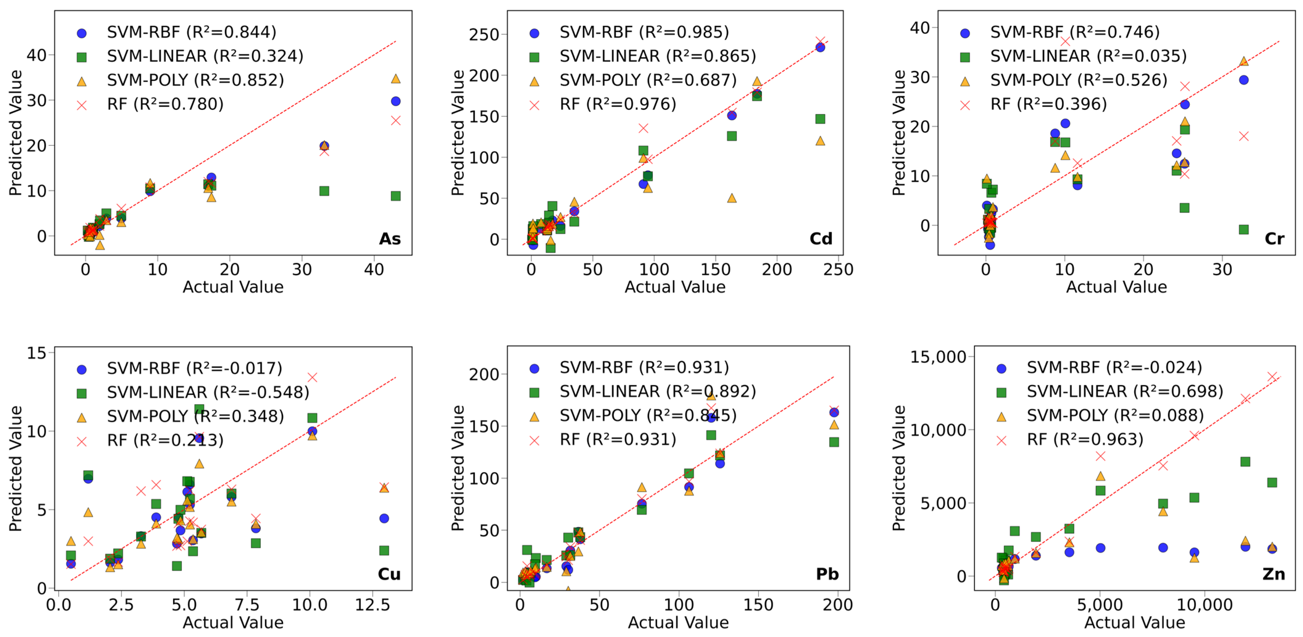
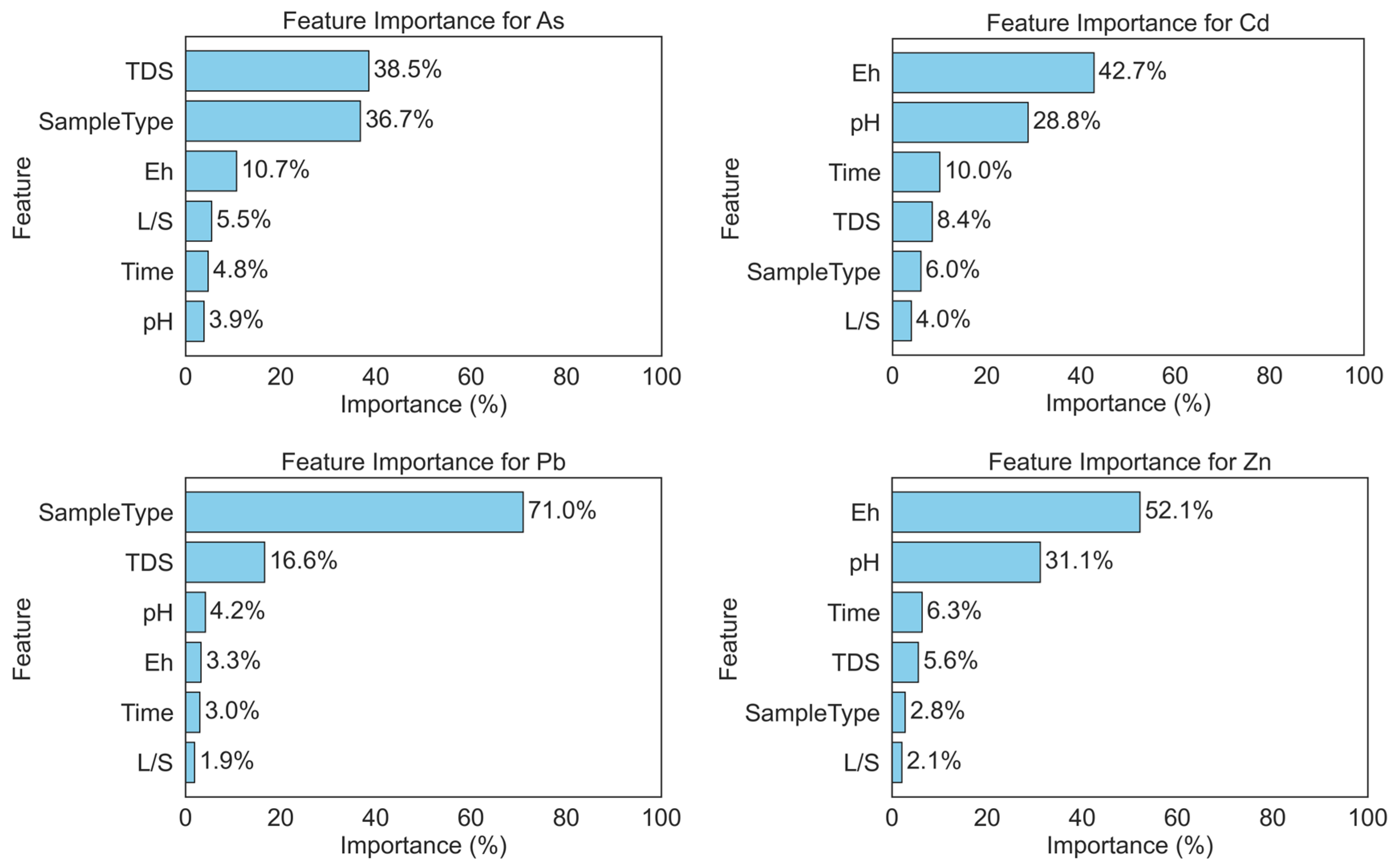
3.6.2. Prediction of Heavy Metal Concentrations Based on Machine Learning

To assess the impact of key environmental factors (pH, Eh, TDS, L/S, time, and sample type) on the migration and release of heavy metals during the experiment, machine learning models were developed to predict heavy metal concentrations using these variables as input features. Two algorithms—Random Forest (RF) and Support Vector Machine (SVM)—were employed and the corresponding results are shown in Figure 11. The coefficient of determination (R²) represents the degree of fit between the predicted values and the observed values. Its value typically ranges from 0 to 1, where a value of 1 indicates a perfect fit, meaning the model’s predictions match the observed data exactly. Conversely, values closer to 0 indicate a poor fit, reflecting a greater discrepancy between the predicted and observed values.

As, Cd, and Pb exhibited good fitting performance in both models, with R² values greater than 0.7. Zn showed a strong fit in the RF model (R² = 0.963), but performed poorly under the SVM model with different kernel functions. In contrast, Cr was better predicted by the SVM model with the RBF kernel (R² = 0.746) than by the RF model (R² = 0.396). However, both models showed poor performance in fitting Cu, with R² values below 0.4. Although SVM theoretically has strong modeling capabilities for nonlinear regression tasks, its performance largely depends on the selection of hyperparameters, especially the type of kernel function [75]. Given that the dataset in this study is relatively small, most elements suffered from overfitting or underfitting in the high-dimensional space of the SVM model. In comparison, the RF model does not rely on kernel functions and requires a simpler parameter-tuning process while maintaining good predictive performance for most elements. These results suggest that the RF model outperforms the SVM model in handling complex nonlinear relationships and noise robustness in small-sample datasets.

Moreover, in machine learning modeling, feature importance analysis serves as a measure of the influence of input variables on model performance—quantifying the individual contribution of each feature to the prediction outcome [76]. Compared with SVM, the RF model has a built-in feature importance evaluation mechanism, which intuitively quantifies the relative contribution of each input variable based on the decision tree splitting criteria. This capability greatly aids in interpreting model outputs and identifying key environmental drivers [77]. Accordingly, feature contribution analysis was conducted for the heavy metals (As, Cd, Pb, and Zn) that exhibited good predictive performance in the RF model. The relative importance of major environmental variables contributing to these heavy metals in the mining area is illustrated in Figure 12.

The results reveal that all environmental factors contributed to the release of heavy metals to varying degrees; however, the sensitivity of heavy metal migration to these factors differed significantly among samples. This indicates varying dependencies on external environmental parameters such as pH, Eh, and TDS.

Specifically, the concentrations of Cd and Zn in leachate were mainly influenced by Eh and pH. For Cd, Eh and pH accounted for 42.7% and 28.8% of the total contribution, respectively, while for Zn, the contributions were 52.1% and 31.1%, respectively. In contrast, the concentrations of As, Cu, and Pb were primarily affected by the sample type. Notably, both TDS and sample type contributed significantly to As and Pb concentrations: 38.5% and 36.7% for As, and 71.0% and 16.6% for Pb, respectively.

These findings demonstrate that the migration and release of heavy metals in the mining area are driven by a complex interplay of multiple environmental and geochemical factors. Machine learning models effectively quantify the relative contributions of these factors, providing a theoretical foundation and technical support for accurate pollution risk assessment and the formulation of targeted remediation strategies.

4. Conclusions

The heavy metal contamination in the soils of the Siding Lead–Zinc mining area is considerable. The results from simulated column leaching experiments under acid rain conditions demonstrated that acid leaching significantly enhances the mobility of heavy metals, with chalcophile elements exhibiting greater migration and release potential than siderophile elements. The primary metals released from different zones into the surrounding environment are Pb, Zn, and Cd, all of which pose potential risks to surface and groundwater quality. It is noteworthy that both the tailings and surrounding soils are rich in carbonate minerals, which can buffer acidification induced by mine drainage and, to some extent, reduce the mobility of heavy metals. Predictive models constructed using Support Vector Machine (SVM) and Random Forest (RF) algorithms successfully captured the variation in heavy metal concentrations in leachate from different sample types under acidic leaching conditions. Furthermore, feature importance analysis allowed for quantitative assessment of the contributions of environmental variables—such as pH, Eh, and TDS—to the observed concentrations of heavy metals in leachate. Therefore, effective environmental management of mine tailings ponds should be guided by the principle of “prevention rather than remediation”. In particular, prior to the rainy season, proactive measures should be taken to inspect and reinforce the structural integrity of tailings pond facilities and wastewater isolation and purification systems should be constructed around the ponds to effectively prevent environmental contamination caused by tailings leakage. At the same time, establishing a systematic pollution monitoring framework and advancing technologies for pollutant removal and ecological restoration are critical for mitigating the ecological risks posed by heavy metal contamination. For example, integrating water chemistry analyses, computer-based simulation, and aeromagnetic monitoring can enable comprehensive tracking of heavy metal migration pathways and facilitate a more accurate assessment of pollution levels in water bodies within mining areas.

References

1. Prakash, J.; Agrawal, S.B.; Agrawal, M. Global Trends of Acidity in Rainfall and Its Impact on Plants and Soil. J. Soil Sci. Plant Nutr. 2023, 23, 398–419. [Google Scholar] [CrossRef] [PubMed]
2. Nieva, N.E.; Borgnino, L.; García, M.G. Long term metal release and acid generation in abandoned mine wastes containing metal-sulphides. Environ. Pollut. 2018, 242, 264–276. [Google Scholar] [CrossRef] [PubMed]
3. Bu, C.; Li, X.; Li, Q.; Li, L.; Wu, P. Spatiotemporal distributions, sources, and health risks of heavy metals in an acid mine drainage (AMD)-contaminated karst river in southwest China. Appl. Water Sci. 2024, 14, 251. [Google Scholar] [CrossRef]
4. Saedpanah, S.; Amanollahi, J. Environmental pollution and geo-ecological risk assessment of the Qhorveh mining area in western Iran. Environ. Pollut. 2019, 253, 811–820. [Google Scholar] [CrossRef] [PubMed]
5. Chalkias, C.; Petrakis, M.; Psiloglou, B.; Lianou, M. Modelling of light pollution in suburban areas using remotely sensed imagery and GIS. J. Environ. Manag. 2006, 79, 57–63. [Google Scholar] [CrossRef]
6. Schiavo, M.; Giambastiani, B.M.; Greggio, N.; Colombani, N.; Mastrocicco, M. Geostatistical assessment of groundwater arsenic contamination in the Padana Plain. Sci. Total Environ. 2024, 931, 172998. [Google Scholar] [CrossRef]
7. Hong, T.; Wang, Z.; Luo, X.; Zhang, W. State-of-the-art on research and applications of machine learning in the building life cycle. Energy Build. 2020, 212, 109831. [Google Scholar] [CrossRef]
8. Huang, G.; Guo, Y.; Chen, Y.; Nie, Z. Application of Machine Learning in Material Synthesis and Property Prediction. Materials 2023, 16, 5977. [Google Scholar] [CrossRef]
9. Vinuesa, R.; Brunton, S. Enhancing computational fluid dynamics with machine learning. Nat. Comput. Sci. 2021, 2, 358–366. [Google Scholar] [CrossRef]
10. Bellinger, C.; Mohomed Jabbar, M.S.; Zaïane, O.; Osornio-Vargas, A. A systematic review of data mining and machine learning for air pollution epidemiology. BMC Public Health 2017, 17, 907. [Google Scholar] [CrossRef]
11. Kida, M.; Pochwat, K.; Ziembowicz, S. Assessment of machine learning-based methods predictive suitability for migration pollutants from microplastics degradation. J. Hazard. Mater. 2024, 461, 132565. [Google Scholar] [CrossRef] [PubMed]
12. Wang, K.; Zhang, C.; Chen, H.; Yue, Y.; Zhang, W.; Zhang, M.; Qi, X.; Fu, Z. Karst landscapes of China: Patterns, ecosystem processes and services. Landsc. Ecol. 2019, 34, 2743–2763. [Google Scholar] [CrossRef]
13. Zaw, K.; Peters, S.G.; Cromie, P.; Burrett, C.; Hou, Z. Nature, diversity of deposit types and metallogenic relations of South China. Ore Geol. Rev. 2007, 31, 3–47. [Google Scholar] [CrossRef]
14. Li, W.; Zhu, T.; Yang, H.; Zhang, C.; Zou, X. Distribution characteristics and risk assessment of heavy metals in soils of the typical karst and non-karst areas. Land 2022, 11, 1346. [Google Scholar] [CrossRef]
15. Chen, H.; Teng, Y.; Lu, S.; Wang, Y.; Wang, J. Contamination features and health risk of soil heavy metals in China. Sci. Total Environ. 2015, 512, 143–153. [Google Scholar] [CrossRef]
16. Li, W.; Deng, Y.; Wang, H.; Hu, Y.; Cheng, H. Potential risk, leaching behavior and mechanism of heavy metals from mine tailings under acid rain. Chemosphere 2024, 350, 140995. [Google Scholar] [CrossRef]
17. Qin, S.; Li, X.; Huang, J.; Li, W.; Wu, P.; Li, Q.; Li, L. Inputs and transport of acid mine drainage-derived heavy metals in karst areas of Southwestern China. Environ. Pollut. 2024, 343, 123243. [Google Scholar] [CrossRef]
18. Liao, J.; Hu, C.; Wang, M.; Li, X.; Ruan, J.; Zhu, Y.; Fairchild, I.J.; Hartland, A. Assessing acid rain and climate effects on the temporal variation of dissolved organic matter in the unsaturated zone of a karstic system from southern China. J. Hydrol. 2018, 556, 475–487. [Google Scholar] [CrossRef]
19. Santona, L.; Castaldi, P.; Melis, P. Evaluation of the interaction mechanisms between red muds and heavy metals. J. Hazard. Mater. 2006, 136, 324–329. [Google Scholar] [CrossRef]
20. Szecsody, J.E.; Truex, M.J.; Qafoku, N.P.; Wellman, D.M.; Resch, T.; Zhong, L. Influence of acidic and alkaline waste solution properties on uranium migration in subsurface sediments. J. Contam. Hydrol. 2013, 151, 155–175. [Google Scholar] [CrossRef]
21. Jurjovec, J.; Blowes, D.W.; Ptacek, C.J.; Mayer, K.U. Multicomponent reactive transport modeling of acid neutralization reactions in mine tailings. Water Resour. Res. 2004, 40. [Google Scholar] [CrossRef]
22. Dold, B.; Fontboté, L. Element cycling and secondary mineralogy in porphyry copper tailings as a function of climate, primary mineralogy, and mineral processing. J. Geochem. Explor. 2001, 74, 3–55. [Google Scholar] [CrossRef]
23. Wu, W.; Qu, S.; Nel, W.; Ji, J. The impact of natural weathering and mining on heavy metal accumulation in the karst areas of the Pearl River Basin, China. Sci. Total Environ. 2020, 734, 139480. [Google Scholar] [CrossRef]
24. Cheng, Q.; Tang, G.; An, J.; Liu, Y. Analysis of acid rain in Liuzhou and its relationship with meteorological conditions. J. Meteorol. Res. Appl. 2018, 39, 75–77+81. [Google Scholar]
25. Cao, J.S.; Shao, Z.Z.; Peng, Z.A.; Zheng, H.; Wei, J.; Nong, S.H. Study on fluid inclusions characteristics of the Siding lead-zinc deposit in Guangxi. Miner. Resour. Geol. 2018, 32, 31–38. [Google Scholar]
26. Lei, L. Mechanism of heavy metals release from carbonate-type tailings in bufferingperiod: Column leaching test. Acta Petrolog. Miner. 2019, 38, 131–142. [Google Scholar]
27. Lei, L.; Song, C.; Wang, F.; Xie, X.; Luo, Y.; Ma, Y. The neutralization capacity and acidification potential of the carbonate-type tailings in north Guangxi and its adjacent areas, South China. J. Miner. Petrol. 2010, 30, 106–113. [Google Scholar]
28. Ministry of Environmental Protection of the People’s Republic of China. The Technical Specification for soil Environmental Monitoring HJ/T 166-2004. 2004. Available online: https://www.mee.gov.cn/image20010518/5406.pdf (accessed on 18 June 2025).
29. State Administration for Market Regulation of the People’s Republic of China. Chemicals—Testing of Leaching in Soil Columns GB/T 41667-2022. 2022. Available online: https://openstd.samr.gov.cn/bzgk/gb/newGbInfo?hcno=56A59C3129E2D32167AD94F485CB3419 (accessed on 18 June 2025).
30. Ministry of Ecology and Environment of the People’s Republic of China. Soil–Determination of pH–Potentiometry HJ 962–2018. 2018. Available online: https://www.mee.gov.cn/ywgz/fgbz/bz/bzwb/jcffbz/201808/W020180815584753007210.pdf (accessed on 18 June 2025).
31. Ministry of Ecology and Environment of the People’s Republic of China. Water Quality—Determination of pH—Electrode Method HJ 1147–2020. 2020. Available online: https://www.mee.gov.cn/ywgz/fgbz/bz/bzwb/shjbh/xgbzh/202011/W020201127577750190580.pdf (accessed on 18 June 2025).
32. Ministry of Environmental Protection of the People’s Republic of China. Water Quality-Determination of Dissolved Oxygen-Electrochemical Probe Method HJ 506–2009. 2009. Available online: https://www.mee.gov.cn/ywgz/fgbz/bz/bzwb/jcffbz/200911/W020111114554879821017.pdf (accessed on 18 June 2025).
33. Zhang, C.Y.; Peng, P.A.; Song, J.Z.; Liu, C.S.; Jue, P.; Lu, P.X. Utilization of modified BCR procedure for the chemical speciation of heavymetals in Chinese soil reference material. Ecol. Environ. Sci. 2012, 21, 1881–1884. [Google Scholar]
34. Ministry of Environmental Protection of the People’s Republic of China. Water Quality—Determination of 65 Elements—Inductively Coupled Plasma-Mass Spectrometry HJ 700-2014. 2014. Available online: https://www.mee.gov.cn/ywgz/fgbz/bz/bzwb/jcffbz/201405/W020140523543423227755.pdf (accessed on 18 June 2025).
35. Haris, H.; Looi, L.; Aris, A.; Mokhtar, N.; Ayob, N.A.A.; Yusoff, F.; Salleh, A.; Praveena, S. Geo-accumulation index and contamination factors of heavy metals (Zn and Pb) in urban river sediment. Environ. Geochem. Health 2017, 39, 1259–1271. [Google Scholar] [CrossRef]
36. Perin, G.; Craboledda, L.; Lucchese, M.; Cirillo, R.; Dotta, L.; Zanette, M.; Orio, A. Heavy metal speciation in the sediments of Northern Adriatic Sea: A new approach for environmental toxicity determination. Heavy Met. Environ. 1985, 2, 454–456. [Google Scholar]
37. Mukherjee, P.; Das, P.K.; Ghosh, P. The extent of heavy metal pollution by chemical partitioning and risk assessment code of sediments of sewage-fed fishery ponds at east Kolkata Wetland, a ramsar site, India. Bull. Environ. Contam. Toxicol. 2022, 108, 731–736. [Google Scholar] [CrossRef]
38. Sundaray, S.K.; Nayak, B.B.; Lin, S.; Bhatta, D. Geochemical speciation and risk assessment of heavy metals in the river estuarine sediments—A case study: Mahanadi basin, India. J. Hazard. Mater. 2011, 186, 1837–1846. [Google Scholar] [CrossRef]
39. State Administration for Market Regulation of the People’s Republic of China. Standards for Drinking Water Quality GB 5749-2022. 2022. Available online: https://openstd.samr.gov.cn/bzgk/gb/newGbInfo?hcno=99E9C17E3547A3C0CE2FD1FFD9F2F7BE (accessed on 18 June 2025).
40. Wasana, H.M.S.; Perera, G.D.R.K.; Gunawardena, P.D.S.; Fernando, P.S.; Bandara, J. WHO water quality standards Vs Synergic effect(s) of fluoride, heavy metals and hardness in drinking water on kidney tissues. Sci. Rep. 2017, 7, 42516. [Google Scholar] [CrossRef] [PubMed]
41. Probst, P.; Wright, M.; Boulesteix, A. Hyperparameters and tuning strategies for random forest. Wiley Interdiscip. Rev. Data Min. Knowl. Discov. 2018, 9, e1301. [Google Scholar] [CrossRef]
42. Tharwat, A. Parameter investigation of support vector machine classifier with kernel functions. Knowl. Inf. Syst. 2019, 61, 1269–1302. [Google Scholar] [CrossRef]
43. Contreras, P.; Orellana-alvear, J.; Muñoz, P.; Bendix, J.; Célleri, R. Influence of Random Forest Hyperparameterization on Short-Term Runoff Forecasting in an Andean Mountain Catchment. Atmosphere 2021, 12, 238. [Google Scholar] [CrossRef]
44. Zhao, Y.; Zhang, W.; Liu, X. Grid search with a weighted error function: Hyper-parameter optimization for financial time series forecasting. Appl. Soft Comput. 2024, 154, 111362. [Google Scholar] [CrossRef]
45. Ali, A.; Gravino, C. An empirical comparison of validation methods for software prediction models. J. Softw. Evol. Process 2021, 33, e2367. [Google Scholar] [CrossRef]
46. Boni, M.; Mondillo, N.; Balassone, G. Zincian dolomite: A peculiar dedolomitization case? Geology 2011, 39, 183–186. [Google Scholar] [CrossRef]
47. Boni, M.; Mondillo, N.; Balassone, G.; Joachimski, M.; Colella, A. Zincian dolomite related to supergene alteration in the Iglesias mining district (SW Sardinia). Int. J. Earth Sci. 2012, 102, 61–71. [Google Scholar] [CrossRef]
48. Ye, Z.; Zhou, J.; Liao, P.; Finfrock, Y.; Liu, Y.; Shu, C.; Liu, P. Metal (Fe, Cu, and As) transformation and association within secondary minerals in neutralized acid mine drainage characterized using X-ray absorption spectroscopy. Appl. Geochem. 2022, 139, 105242. [Google Scholar] [CrossRef]
49. Moncur, M.C.; Ptacek, C.J.; Blowes, D.W.; Peterson, R.C. The occurrence and implications of efflorescent sulfate minerals at the former Sherritt–Gordon Zn–Cu Mine, Sherridon, Manitoba, Canada. Can. Mineral. 2015, 53, 961–977. [Google Scholar] [CrossRef]
50. Bidari, E.; Aghazadeh, V. Pyrite oxidation in the presence of calcite and dolomite: Alkaline leaching, chemical modeling and surface characterization. Trans. Nonferrous Met. Soc. China 2018, 28, 1433–1443. [Google Scholar] [CrossRef]
51. Yang, Z.; Peng, M.; Zhao, C. The study of geochemical background and base line for 54 chemical indicators in Chinese soil. Earth Sci. Front. 2024, 31, 380–402. [Google Scholar]
52. Mbey, J.A.; Thomas, F.; Razafitianamaharavo, A.; Caillet, C.; Villiéras, F. A comparative study of some kaolinites surface properties. Appl. Clay Sci. 2019, 172, 135–145. [Google Scholar] [CrossRef]
53. Lim, J.E.; Ahmad, M.; Lee, S.S.; Shope, C.L.; Hashimoto, Y.; Kim, K.; Usman, A.R.; Yang, J.E.; Ok, Y.S. Effects of lime-based waste materials on immobilization and phytoavailability of cadmium and lead in contaminated soil. Clean–Soil Air Water 2013, 41, 1235–1241. [Google Scholar] [CrossRef]
54. Luo, K.; Liu, H.; Liu, Q.; Tu, Y.; Yu, E.; Xing, D. Cadmium accumulation and migration of 3 peppers varieties in yellow and limestone soils under geochemical anomaly. Environ. Technol. 2022, 43, 10–20. [Google Scholar] [CrossRef]
55. Sorrentino, G.P.; Guimarães, R.; Valentim, B.; Bontempi, E. The influence of liquid/solid ratio and pressure on the natural and accelerated carbonation of alkaline wastes. Minerals 2023, 13, 1060. [Google Scholar] [CrossRef]
56. Bonnissel-gissinger, P.; Alnot, M.; Ehrhardt, J.; Behra, P. Surface oxidation of pyrite as a function of pH. Environ. Sci. Technol. 1998, 32, 2839–2845. [Google Scholar] [CrossRef]
57. Daniels, W.L.; Zipper, C.E.; Orndorff, Z.; Skousen, J.; Barton, C.D.; Mcdonald, L.M.; Beck, M.A. Predicting total dissolved solids release from central Appalachian coal mine spoils. Environ. Pollut. 2016, 216, 371–379. [Google Scholar] [CrossRef]
58. Marguš, M.; Morales-reyes, I.; Bura-nakić, E.; Batina, N.; Ciglenečki, I. The anoxic stress conditions explored at the nanoscale by atomic force microscopy in highly eutrophic and sulfidic marine lake. Cont. Shelf Res. 2015, 109, 24–34. [Google Scholar] [CrossRef]
59. Skousen, J.G.; Sexstone, A.; Ziemkiewicz, P.F. Acid mine drainage control and treatment. Reclam. Drastically Disturb. Lands 2000, 41, 131–168. [Google Scholar]
60. Standardization Administration of the People’s Republic of China. Standard for Groundwater Quality GB/T 14848-2017. 2017. Available online: https://openstd.samr.gov.cn/bzgk/gb/newGbInfo?hcno=F745E3023BD5B10B9FB5314E0FFB5523 (accessed on 18 June 2025).
61. Perera, T.; Mcgree, J.; Egodawatta, P.; Jinadasa, K.; Goonetilleke, A. New conceptualisation of first flush phenomena in urban catchments. J. Environ. Manag. 2021, 281, 111820. [Google Scholar] [CrossRef] [PubMed]
62. Lau, S.; Han, Y.; Kang, J.; Kayhanian, M.; Stenstrom, M. Characteristics of Highway Stormwater Runoff in Los Angeles: Metals and Polycyclic Aromatic Hydrocarbons. Water Environ. Res. 2009, 81, 308–318. [Google Scholar] [CrossRef]
63. Wang, P.; Sun, Z.; Hu, Y.; Cheng, H. Leaching of heavy metals from abandoned mine tailings brought by precipitation and the associated environmental impact. Sci. Total Environ. 2019, 695, 133893. [Google Scholar] [CrossRef]
64. Greenacre, M.; Groenen, P.J.F.; Hastie, T.; D’enza, A.I.; Markos, A.; Tuzhilina, E. Principal component analysis. Nat. Rev. Methods Primers 2022, 2, 100. [Google Scholar] [CrossRef]
65. Jurjovec, J.; Ptacek, C.J.; Blowes, D.W. Acid neutralization mechanisms and metal release in mine tailings: A laboratory column experiment. Geochim. Cosmochim. Acta. 2002, 66, 1511–1523. [Google Scholar] [CrossRef]
66. Liu, Y.Z.; Xiao, T.; Zhu, Z.; Ma, L.; Li, H.; Ning, Z. Geogenic pollution, fractionation and potential risks of Cd and Zn in soils from a mountainous region underlain by black shale. Sci. Total Environ. 2020, 760, 143426. [Google Scholar] [CrossRef]
67. Markiewicz-patkowska, J.; Hursthouse, A.; Przybyla-kij, H. The interaction of heavy metals with urban soils: Sorption behaviour of Cd, Cu, Cr, Pb and Zn with a typical mixed brownfield deposit. Environ. Int. 2005, 31, 513–521. [Google Scholar] [CrossRef]
68. Li, X.; Zhou, T.; Li, Z.; Wang, W.; Zhou, J.; Hu, P.; Luo, Y.; Christie, P.; Wu, L. Legacy of contamination with metal (loid) s and their potential mobilization in soils at a carbonate-hosted lead-zinc mine area. Chemosphere 2022, 308, 136589. [Google Scholar] [CrossRef]
69. Stoessell, R.K.; Moore, Y.H.; Coke, J.G. The occurrence and effect of sulfate reduction and sulfide oxidation on coastal limestone dissolution in Yucatan cenotes. Groundwater 1993, 31, 566–575. [Google Scholar] [CrossRef]
70. Zhang, X.; Tong, J.; Hu, B.; Wei, W. Adsorption and desorption for dynamics transport of hexavalent chromium (Cr(VI)) in soil column. Environ. Sci. Pollut. Res. 2017, 25, 459–468. [Google Scholar] [CrossRef] [PubMed]
71. Zhang, D.; Liu, X.; Ding, Y.; Liu, J.; Jiang, H.; Dong, H. Enhanced oxidation of Cr (III)–Fe (III) hydroxides by oxygen in dark and alkaline environments: Roles of Fe/Cr ratio and siderophore. Environ. Sci. Technol. 2023, 57, 13172–13181. [Google Scholar] [CrossRef]
72. Löv, Å.; Sjöstedt, C.; Larsbo, M.; Persson, I.; Gustafsson, J.P.; Cornelis, G.; Kleja, D.B. Solubility and transport of Cr (III) in a historically contaminated soil–evidence of a rapidly reacting dimeric Cr (III) organic matter complex. Chemosphere 2017, 189, 709–716. [Google Scholar] [CrossRef]
73. Griffin, R.; Au, A.K.; Frost, R. Effect of pH on adsorption of chromium from landfill-leachate by clay minerals. J. Environ. Sci. Health Part A 1977, 12, 431–449. [Google Scholar] [CrossRef]
74. Xu, T.; Nan, F.; Jiang, X.; Tang, Y.; Zeng, Y.; Zhang, W.; Shi, B. Effect of soil pH on the transport, fractionation, and oxidation of chromium(III). Ecotoxicol. Environ. Saf. 2020, 195, 110459. [Google Scholar] [CrossRef]
75. Raj, J.; Ananthi, V. Recurrent neural networks and nonlinear prediction in support vector machines. J. Soft Comput. Paradig. 2019, 2019, 33–40. [Google Scholar] [CrossRef]
76. Saarela, M.; Jauhiainen, S. Comparison of feature importance measures as explanations for classification models. SN Appl. Sci. 2021, 3, 272. [Google Scholar] [CrossRef]
77. Gregorutti, B.; Michel, B.; Saint-Pierre, P. Correlation and variable importance in random forests. Stat. Comput. 2013, 27, 659–678. [Google Scholar] [CrossRef]
Figure 1. Configuration of sample and column experiment. (A) Schematic diagram of the sampling area; (B) schematic diagram of the column experiment setting.
Minerals 15 00663 g001
Figure 2. Backscattered electron images and X-ray diffraction patterns of different samples. (A) Tailings; (B) dolomite-rich red soil; (C) river sediment; (D) clay-rich red soil. Dol, dolomite; Cc, calcite; Qz, quartz; clay, clay mineral; Py, pyrite; Cer, cerussite; Sp, sphalerite.
Minerals 15 00663 g002
Figure 3. X-ray diffraction patterns of different samples. (A,B) XRD patterns of different samples before and after leaching tests. 1, CaSO4·2H2O; 2, SiO2, Qz, quartz; 3, CaCO3, Cc, calcite; 4, CaMg(CO3)2 /CaZn(CO3)2, Dol, dolomite; 5, FeS2, Sp, sphalerite; 6, Al2Si4O10(OH)2; 7, Mg2Al(AlSi3O10)(OH)2·4H2O; 8, Mg5Al(Si,Al)4O10(OH)8.
Minerals 15 00663 g003
Figure 4. Bar chart of heavy metal speciation distribution in the tested samples. (A) Geo-accumulation Index of the Samples; (BG) Chemical fractions of As, Cd, Cr, Cu, Pb, and Zn, respectively. (H) Risk Assessment Code of the Samples; F1, acid-soluble fraction; F2, fraction; F3, oxidizable fraction; F4, residual fraction.
Minerals 15 00663 g004
Figure 5. The pH, Eh, and TDS values in leachates from different samples. (A) the pH value; (B) the Eh value; (C) the TDS value.
Minerals 15 00663 g005
Figure 6. Concentration of heavy metals in leachate from different samples.
Minerals 15 00663 g006
Figure 7. Cumulative release mass of heavy metals in leachate from different samples.
Minerals 15 00663 g007
Figure 8. The total mass of heavy metals released from different samples and its relationship with L/S ratio and time. (A) N1; (B) N2; (C) N3; (D) N4; (E) N5.
Minerals 15 00663 g008
Figure 9. WQI values of leachates from different samples.
Minerals 15 00663 g009
Figure 10. Principal component analysis of different environmental factors and heavy metals. (A) Heatmap of correlation coefficients for PC1~PC4; (B) three-dimensional PCA biplot showing the distribution of samples in the principal component space (PC1~PC3) and the loading directions of each variable.
Minerals 15 00663 g010
Figure 11. Model validation: predicted vs. actual heavy metal concentrations.
Minerals 15 00663 g011
Figure 12. Feature importance for heavy metal release prediction based on an RF algorithm.
Minerals 15 00663 g012