A Study on the Imaging Method for the Channel Wave Dispersion Curve Variability Function

Abstract

When the channel wave passes through the abnormal body, the dispersion curve appears interval, dislocation, and discontinuity, resulting in the non-standard and large error of the “velocity-frequency” pickup result of the transmitted channel wave dispersion curve, which directly leads to the inaccurate tomography. Therefore, aiming at this problem, the imaging method of dispersion curve variability function is proposed: (1) count the breakpoints of dispersion curve according to three types; (2) set the weighting factor for the breakpoint according to the spectrum curve; (3) the variability function is constructed for the dispersion curve, and the corresponding variation value is obtained; and (4) the variability value is back projected into the imaging grid space to obtain the abnormal body information in the detection area. The example verification results show that the imaging results of this method are accurate and stable, and non-convergence is caused by cyclic iteration, which provides a new imaging mode for the detection of complex structures in coal seams.

1. Introduction

Channel wave seismic detection is a geophysical method that utilizes guided waves formed after multiple reflections in coal seams to detect coal seam structure and lithological changes [1,2]. It has advantages that include a large detection range, high precision, strong anti-interference, and easy recognition of waveform features. Therefore, the channel wave detection technique has gradually become an optimal choice for detecting abnormal bodies, such as faults, collapse columns, dirt bands, and others in underground coal mines [3,4]. There are two stages of progress in the application of channel wave seismic detection techniques in the 21st century. The first phase is the Feasibility Plan for Goaf Geophysical Detection launched by the United States in 2001 that included four research projects that focused on channel wave detection, which has greatly promoted the development of channel wave exploration [5]. The second phase is the key projects supported by the National Natural Science Foundation and led by Teng from 2012, which were critical in leading channel wave study in China, greatly promoting the development of channel wave forward modelling and dispersion curve characters, multiple tomographic imaging methods, applications for channel wave technology, and many other aspects [6,7,8,9].

Seismic waves usually travel slower in coal seams than in the surrounding upper and lower rocks. When seismic waves are excited in a coal seam, they spread into the surrounding rocks in the coal seam. As they travel faster in the surrounding rocks than in the coal seam, transmitted waves and reflected waves are generated when the wave rays encounter the interfaces between the coal seam and the surrounding rocks. When the incident angle exceeds the critical angle, total reflection occurs. The seismic waves then propagate and interfere with each other in the coal seam, thus forming channel waves with dispersion characteristics. Their dispersion curves are related not only to the velocity in the upper and lower surrounding rocks and the velocity in and the thickness and density of the coal seams but also to the types, locations, sizes, and shapes of any abnormal bodies they pass through [10,11,12]. Yanhui Wu used the ellipse tangent method and transmission tomography information to obtain the interpretation results for channel waves and statistically analyzed the quantity, extended length, and direction of faults interpreted by structure development rules and 3D seismic techniques, further reasonably inferring internal and external distributions and the extended lengths of channel wave detection faults in the working faces [13]. Based on the homogeneity and isotropy condition of the coal seam, Cox and Mason used five different methods to analyze the dispersion of Schwalbach coal mine data and obtained the advantages and differences of different methods. At the same time, it has been proved that the slight discrepancy between theoretical and actual dispersion characteristics could be reduced by increasing the model’s complexity [14]. Hu used wave equation reverse time migration imaging technology to image faults and voids in coal seams in 2D model data and to effectively distinguish fluids in mine voids from seismic data [15]. Ge made use of the wide frequency channel wave in the thin coal seam (1.4 m on average), with a frequency of 50 to 5000 Hz, and found that the Airy phase had a typical frequency range of 400–600 Hz with a fairly stable velocity of 975 m/s [16]. By using wavelet transform, the dispersion characteristics of channel wave velocity varying with frequency in thin coal seam are obtained, and the examples prove that the attenuation characteristics of channel wave low frequency can effectively identify goaf and faults in coal seam [17]. Hu analyzed the relationship between the depth and energy distribution of multi-order Love-type channel waves and the group velocity dispersion curve by time–frequency analysis and obtained the phase velocity dispersion curve based on the mathematical relationship between the group and phase velocities [18]. Ji found that the difference between the basic order Rayleigh dispersion curves of vertically anisotropic media and isotropic media is small by analyzing the model data, whereas the difference between the dispersion curves of higher-order modes is large. The difference between the horizontal transversely isotropic medium (HTI) and the isotropic medium is large [19].

Transmission detection usually adopts dispersion curves to determine the traveling velocity (travel time) tomography of the transmitted wave [20,21]. However, when dispersion curves are used for determining travel time or velocity, their shapes will be affected by the coal seam thickness and wave velocity and by any abnormal bodies on the ray path of channel waves [22,23,24]. When channel waves pass through an abnormal body, the dispersion curves have poorer continuity and are not smooth, making the accurate determination of the travel time impossible and leading to difficulty in determining the travel time based on a fixed frequency. In channel wave tomography, the travel time (velocity) of the Airy phase or the travel time (velocity) information of a certain frequency seismic phase is picked up from the dispersion curve. The inversion calculation algorithm using tomography is as follows [25,26,27]: Back projection method (BG), conjugate gradient method (CG), Least square QR-factorization (LSQR), Algebraic reconstruction technique (ART), simultaneous iterative reconstruction technique (SIRT), etc. The results of these inversion methods are only relative, and the result values are through to the velocity information of the dispersion curve within the thickness range of coal seam for theoretical inversion. However, it is difficult to determine the degree of influence of geological anomalies on the dispersion characteristics. In actual detection work, determining travel time on complex coal faces is an important link that causes issues for processing personnel. Lacking a unified standard for determining velocity, the imaging results are inconsistent and inaccurate [28,29,30]. To solve the aforementioned imaging problems, this paper proposes a function that is based on the quantitative description and calculates the variation degrees of dispersion curves and utilizes the tomography method to identify abnormal bodies.

2. Variability Function Method

2.1. Definition of Variability Function

A seismic wave that is excited in the low-velocity coal seam propagates in all directions, encountering the surrounding upper and lower high-velocity rock mass media, resulting in transmission and reflection. When the incident angle exceeds the critical angle, total reflection occurs, and the total reflection wave is reflected by the upper and lower surrounding rocks into the coal seam and propagates forward, forming a channel wave with dispersion characteristics [31,32]. When the channel wave propagates forward, it encounters abnormal bodies, such as collapse columns, faults, and goaves, resulting in changes in the total reflection conditions of the channel wave, leading to intermittent, erratic, and discontinuous channel wave dispersion curves, forming irregular dispersion curves [33,34] that are defined as variance dispersion curves, and the degree of variance is expressed in terms of variability. The number of discontinuity points of the dispersion curve and the corresponding velocity and frequency are used as independent variables to construct a variability function indicating the variation magnitude.

A dispersion curve can be extracted from the transmitted waves received in the underground roadway using narrow band filtering or wavelet transformation. When the transmitted channel wave does not pass through abnormal bodies, the dispersion curve is a continuous smooth curve, close to the theoretically calculated dispersion curve, as shown in Figure 1a. When the transmitted channel wave passes through abnormal bodies, the dispersion curve appears to be intermittent and is an irregular variation curve, as shown in Figure 1b. The velocity in the figure is the ratio of the ray path length to the travel time; thus, the distribution of the velocity values is unequal [35].

2.2. Breaking Point Classification

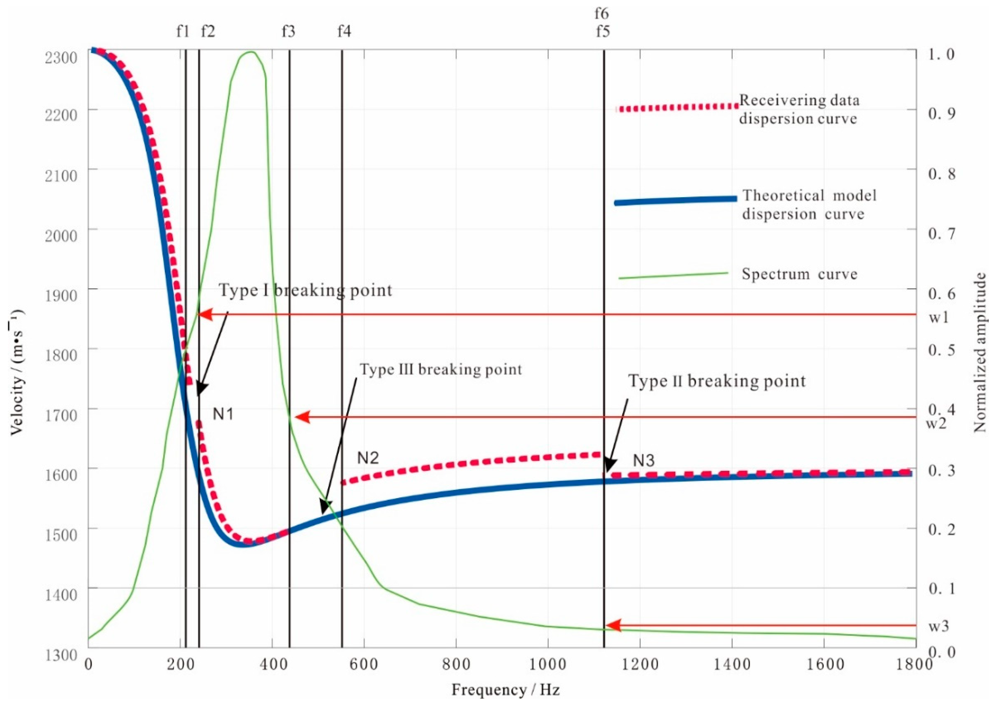
Comparing the variance dispersion curve with the theoretical dispersion curve (blue curve in Figure 2), the breaking points can be classified into three categories according to the discontinuity of the variance curve: Type I breaking point, in which the variance dispersion curve is intermittent (the frequency is not continuous) but is consistent with the shape of the theoretical dispersion curve (N1 in Figure 2); Type II breaking point, in which the variance dispersion curve is staggered vertically, but the frequency is continuous (N3 in Figure 2); and Type III breaking point, in which the variance dispersion curve is erratic vertically, and the frequency is not continuous (N2 in Figure 2). The dispersion curves are extracted for each transmission channel wave, and the breaking point type of all dispersion curves are identified and the total number of breaking points, N, is counted. Two frequency values are specified at each breaking point. Then, the corresponding frequency values at the $i$th breaking point are $f_{2i-1},f_{2i}$, and $f_{2i-1}\le f_{2i}$. The frequency at the breaking point and the corresponding velocity change information reflect the magnitude of the dispersion curve variability.

2.3. Weighting Factor

In the variability function, the breaking point position is related to channel wave energy; thus, the normalized amplitude value corresponding to the breaking point position is set as a weighting factor. The Fourier transformation of the channel wave data is performed, and the amplitudes are normalized to superimpose the spectral curve onto the dispersion curve (green spectral curve in Figure 2).

The three breaking points (N1, N2, N3) in the figure correspond to the three types of breaking points. N1 corresponds to the first type of breaking point and corresponds to two frequencies, f₁ and f₂. The maximum value in the normalized amplitude of f₁ and f₂ in the spectrum curve is the weighting factor w₁. Similarly, the weighting factors w₂ and w₃ corresponding to the breaking points N2 and N3 are obtained. That is, the maximum value in the spectrum corresponding to the two frequencies $f_{2i-1}$ and $f_{2i}$ in the ith breaking point of the actual dispersion curve is the weighting factor for that breaking point. From the spectrum curve, the main frequency of the channel wave $f_m$, and $f_a$ and $f_b$, which are 0.1 times the amplitudes of the main frequency, are obtained. The difference between them is the spectrum band.

2.4. Construction of the Variability Function

Based on the definition of dispersion curve variability, Equation (1) for the variability for each transmitted channel wave is constructed as

$$d_{S_j{R}_k}(v,f,n)={\sum }_{i=1}^N{w}_i|\frac{{v^{\prime }}_{2i}-V_{2i}}{V}|+{\sum }_{i=1}^N{w}_i|\frac{f_{2i}-f_{2i-1}}{F}|$$

(1)

where $d$ is the variability, R is the receiver point ($k=1, 2 \dots , K$), S is the source point ($j$ = 1, 2, ……, J) (Figure 3), the total number of breaking points is N, $i$ is the -ith breaking point, $w$ is the weighting factor at the breaking point, $V$ is the transverse wave velocity of the surrounding rock, F is the maximum frequency $f_b$ corresponding to the main frequency interval, $v_{2i}$ is the actual velocity value at frequency $f_{2i}$ in the ith breaking point, and${v^{\prime }}_{2i}$ is the theoretical calculated velocity value at frequency $f_{2i}$in the ith breaking point.

The first term to the right of the equal sign in Equation (1) indicates the magnitude of the contribution of velocity (time) intermittency to the variability value, and the second term indicates the magnitude of the frequency intermittency contribution to the variability value.

According to the breaking point classification, the first and second terms in the equation take the values of the following:

In a Type I breaking point, the curve is consistent with the shape of the theoretical dispersion curve. Only the frequency f is intermittent and extended consistently with the theoretical frequency. According to the theoretical equation, $f_{2i} \mathrm{corresponds} \mathrm{to} \mathrm{the} \mathrm{velocity} {v^{\prime }}_{2i}$, and ${v^{\prime }}_{2i}=v_{2i}$, ($v_{2i}$ is the velocity corresponding to the dispersion curve of the received data) when the first term in Equation (1) is 0, the second term is not 0.

In a Type II breaking point, the curve is erratic up and down, but the frequency f is continuous. According to the theoretical equation, $f_{2i}$ corresponds to ${v^{\prime }}_{2i}$, with ${v^{\prime }}_{2i}\ne v_{2i}$ ($v_{2i}$ is the maximum velocity of frequency f corresponding to the dispersion curve of received data), when the first term in the Equation (1) is not equal to 0, and the second term is 0.

In a Type III breaking point, the curve is erratic vertically, and the frequency f is intermittent. According to the theoretical equation, $f_{2i}$ corresponds to ${v^{\prime }}_{2i}$, with ${v^{\prime }}_{2i}\ne v_{2i}$. At this time, the first and second terms in Equation (1) are not 0.

Equation (1) indicates that a greater number of breaking points leads to greater variability; a larger value for d leads to a greater variability value and a greater influence of geologically abnormal bodies, whereas a smaller d leads to less variability and less influence from geologically abnormal bodies. The variability value of the channel wave ray path is 0 when it does not pass through any abnormal bodies. The variability values for the channel wave data are calculated using Equation (1).

2.5. Variability Function Imaging

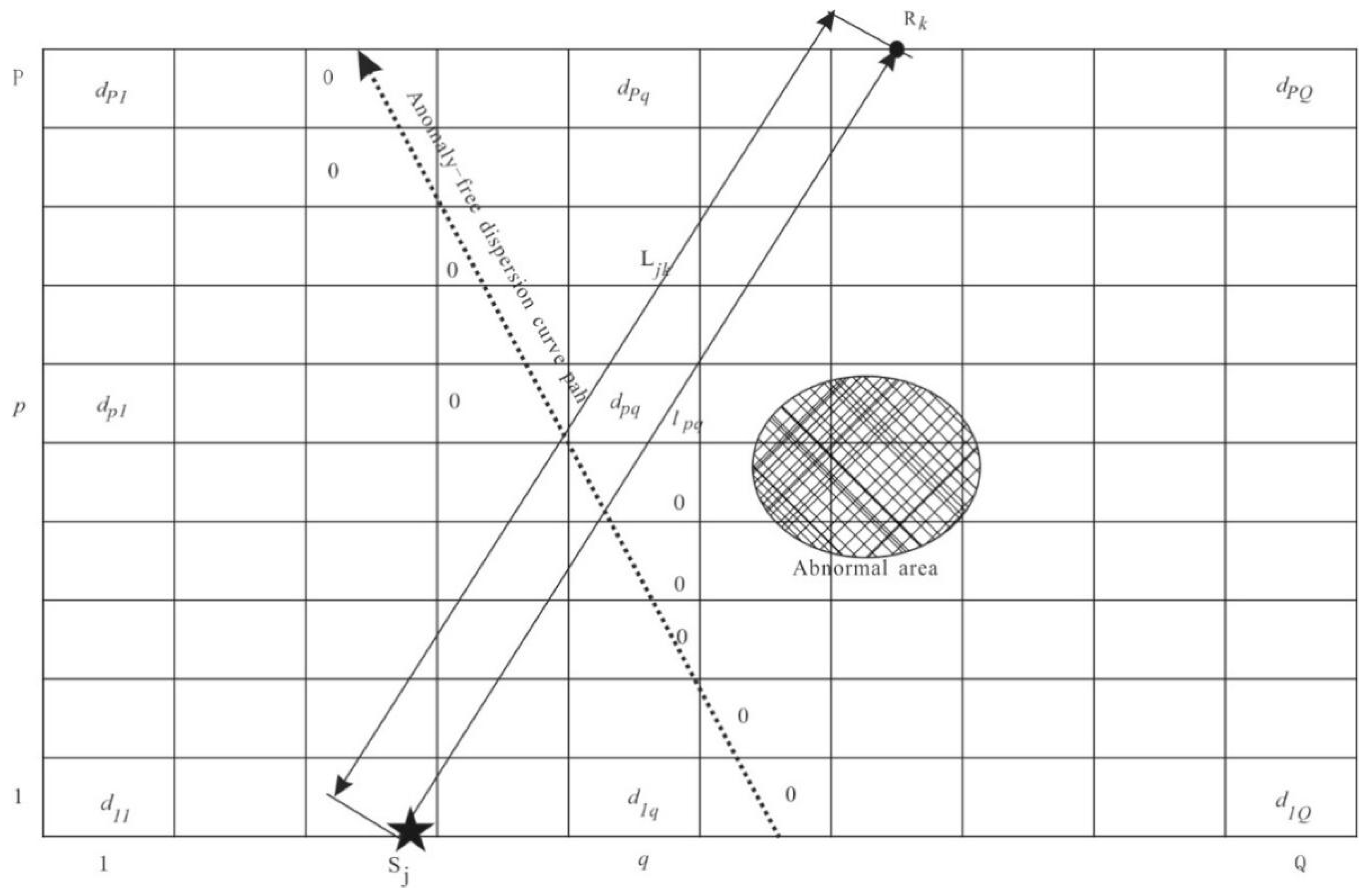
The detection area is dissected into a rectangular grid, as shown in Figure 3. In this figure, the receiver and source points are located in different lanes, and the channel wave ray path length is the distance L from the source point to the receiver point, and the variability is discretized by the grid. The theoretical dispersion curve variability value is determined by the length of the ray passing through the grid point and the grid point variability value, using Equation (2):

$$d_{jk}{}^t=\sum _{p=1}^P(\frac{l_{pq}^{jk}}{L_{jk}}\times d_{pq}),$$

(2)

where $d_{jk}{}^t$ is the theoretical calculated value of the dispersion curve variability of the channel wave at the jth source point and the kth receiver point, $L_{jk}$is the length of the channel wave path at the jth source point and the kth receiver point, ${l_{pq}^{jk}}_{jk}$is the length of the grid point in row p and column q through which the channel wave at the jth source point and the kth receiver point passes, and $d_{pq}$ is the value of the grid point variability in row p and column q.

Each transmitted channel wave variability value and the theoretical calculated value form the system of Equation (3), and the system of binary linear equations is solved under the least squares conditions to obtain the grid point variability values.

$$\left\{\begin{array}{c}{d}_{S_1{R}_1}={\displaystyle \sum _{p=1}^P}(\frac{l_{pq}^{11}}{L_{11}}\times d_{pq})\\ d_{S_1{R}_2}={\displaystyle \sum _{p=1}^P}(\frac{l_{pq}^{12}}{L_{12}}\times d_{pq})\\ ⋮\\ d_{S_j{R}_k}={\displaystyle \sum _{p=1}^P}(\frac{l_{pq}^{jk}}{L_{jk}}\times d_{pq})\\ ⋮\\ d_{S_J{R}_{K-1}}={\displaystyle \sum _{p=1}^P}(\frac{l_{pq}^{JK-1}}{L_{JK-1}}\times d_{pq})\\ d_{S_J{R}_K}={\displaystyle \sum _{p=1}^P}(\frac{l_{pq}^{JK}}{L_{JK}}\times d_{pq})\end{array}.\right.$$

(3)

As can be determined by the application of Equation (1), when the dispersion curve is smooth and continuous, its variance value is 0. Since the defined variability value is greater than or equal to 0, and the grid points through which the slotted wave rays pass have a variability value of 0, the variability value for this grid point in the corresponding initial model is 0, thus reducing the number of unknown solutions to Equation (3). The abnormal-free dispersion curve shown in Figure 3 has a variability value of 0 through the path grid. When using travel time (velocity) tomography, the velocity value magnitudes of the grid points on the same ray path vary, and the total ray travel time is obtained by accumulating the travel times of the grid points; thus, the initial model velocities are unknown. Theoretically, the variability function tomography has fewer unknowns and fewer equations and is computationally efficient.

The solution process: (1) according to the channel wave ray path, the variation value is allocated to the grid points passing by, the initial variation model is obtained, and the theoretical grid point variation value is calculated; thus, (2) calculate the variation correction amount of ray passing through each grid area; (3) add the above results to the initial variability to generate a new variability; (4) and the variation value shall be recalculated and compared with the actual variation value until the minimum error condition is met.

3. Example

3.1. Introduction to the Work Area and Data Collection

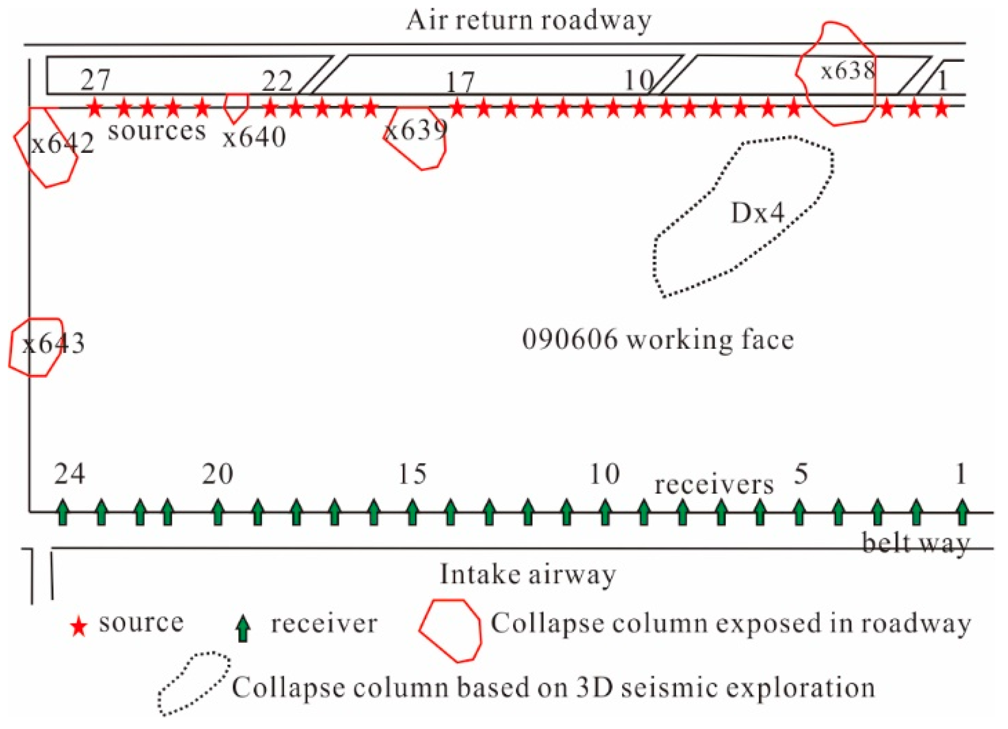
The above method was applied to a channel wave detection example. The work area of the channel wave seismic detection is a Mine 090606 working face (Figure 4) that has a stable coal seam thickness of 4.1–4.3 m. The working face roadway revealed five collapse columns in Figure 4 marked with red circles, plus one collapse column determined from 3D seismic speculation in Figure 4 marked with dotted line. The abnormal body detection target is the collapse column. According to the detection task, 27 source points and 24 receiver points were set up in the upper and lower lanes of the working face, respectively, with the source point distance being 10 m and the receiver point distance being 15 m. SUMMIT-II channel wave seismic recording and double-component velocity detectors were used for the receiver.

The red stars mark source point locations, and the green arrows mark the receiver point locations.

3.2. Data Processing

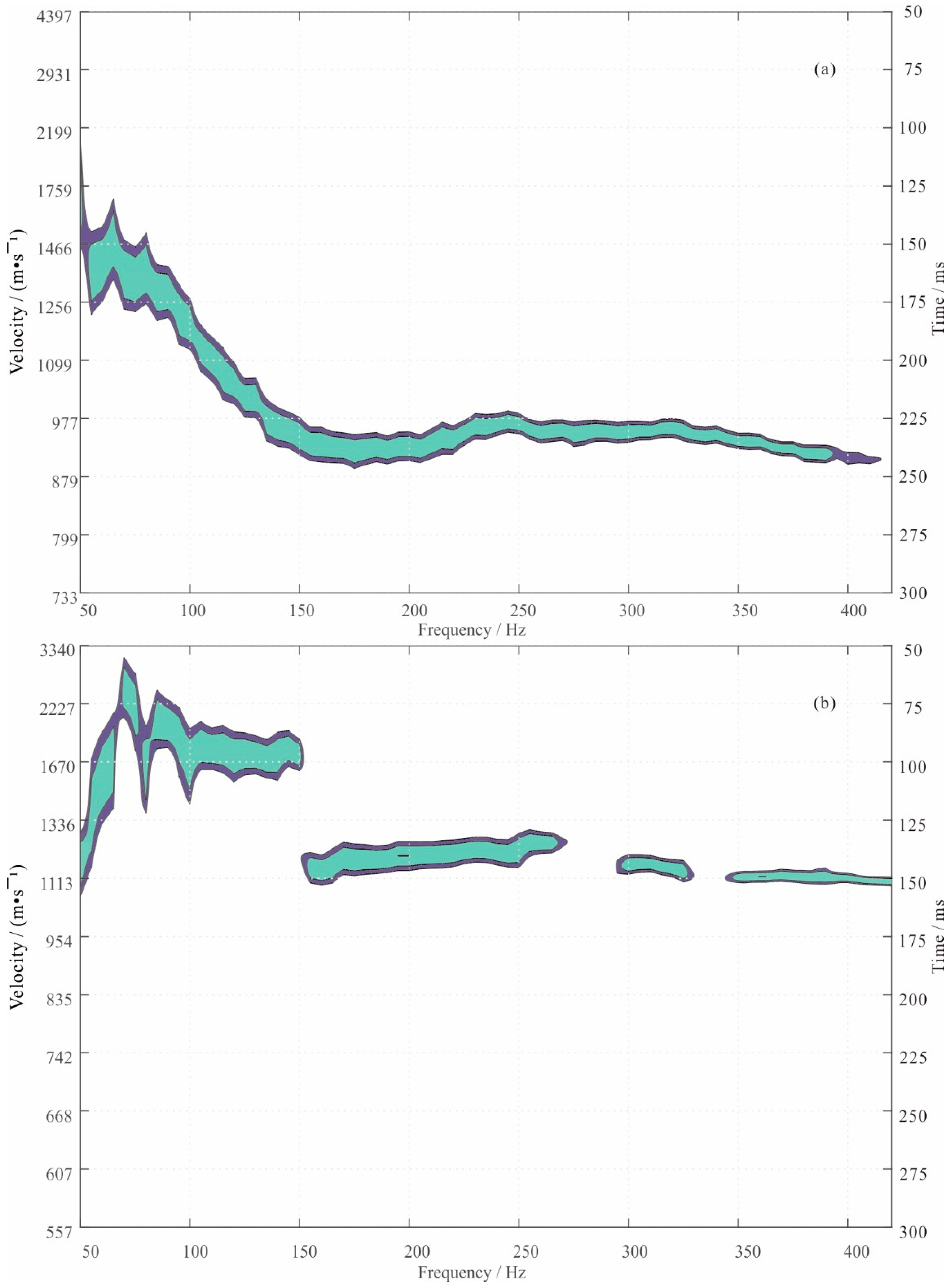
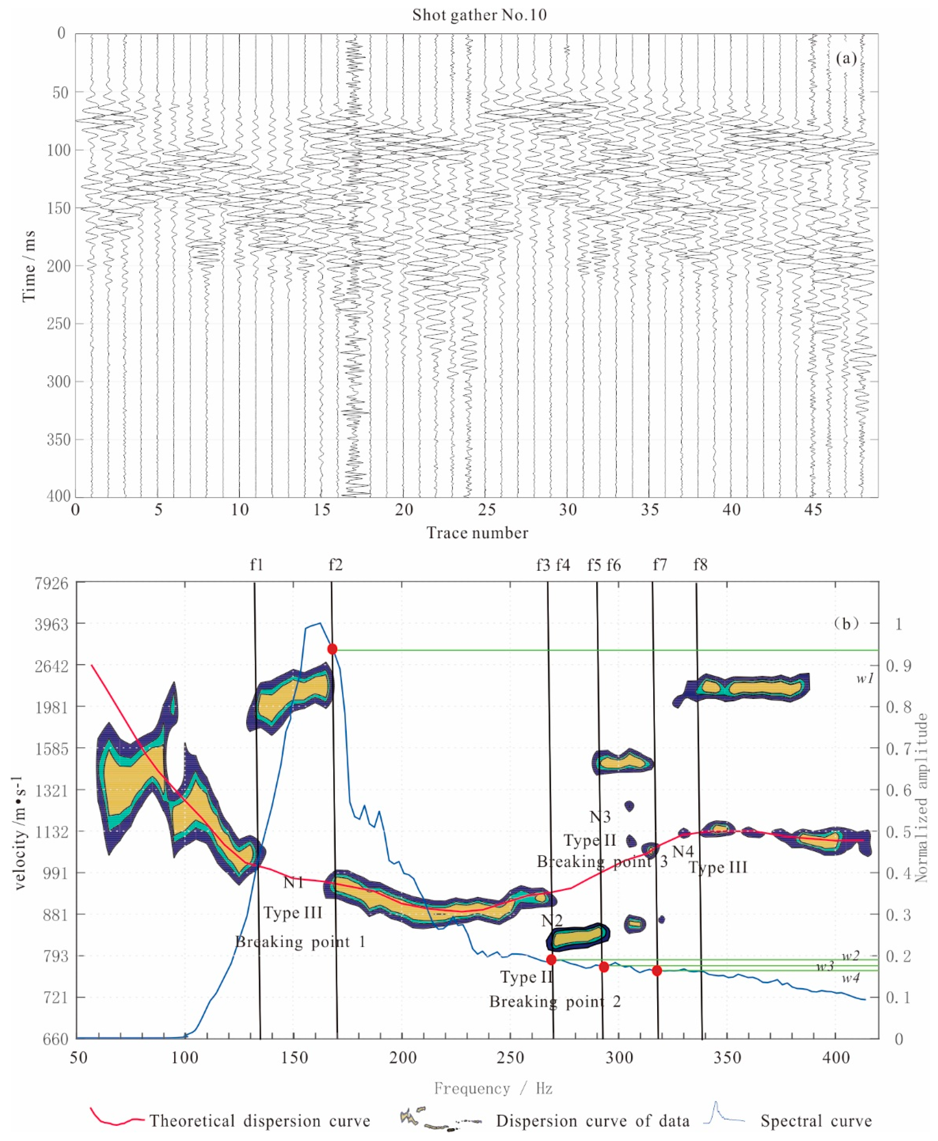
Direct P-wave, S-wave, and channel wave signals can be identified from the seismic records (Figure 5a). Dispersion analysis and spectral analysis of the channel waves were conducted by the dispersion curve variability method to determine the type of breaking point and its weighting factor in the spectral curve (Figure 5b). For the theoretical dispersion curve calculation, a smooth and continuous dispersion curve from the actual channel seismic record was used (Figure 5b red curve). In Figure 5b, the fa is 110 Hz, fb is 410 Hz, and the F is 300 Hz, the V is the S velocity, 2600 m/s. The path length is 198.8 m (shot No. 10 with receiver No. 18), and the variability parameters for the nth trace of the nth source are shown in

Table 1. Variability Parameters.

Breaking Point Number	Breaking Point Type	Theoretical Breaking Point Velocity (m/s) /Time (ms)	Practical Breaking Point Velocity (m/s) and Time (ms)	Breaking Point Frequency1 (Hz)	Breaking Point Frequency2 (Hz)	Weighting Factor
1	III	967/205.5	2298/86.5	135	170	0.935
2	II	929/214	808/246	270	270	0.190
3	II	947/210	824/241	292	292	0.175
4	III	1156/172	2185/91	319	349	0.160

.

In the actual calculation of the variation value, we do not need to identify the breakpoint type but only need to extract the frequency, velocity, normalized amplitude value of the corresponding frequency, and the velocity value at the breakpoint of the theoretical dispersion curve, and we bring these parameters into the calculation Equation (1) for automatic identification and calculation.

3.3. Imaging Results

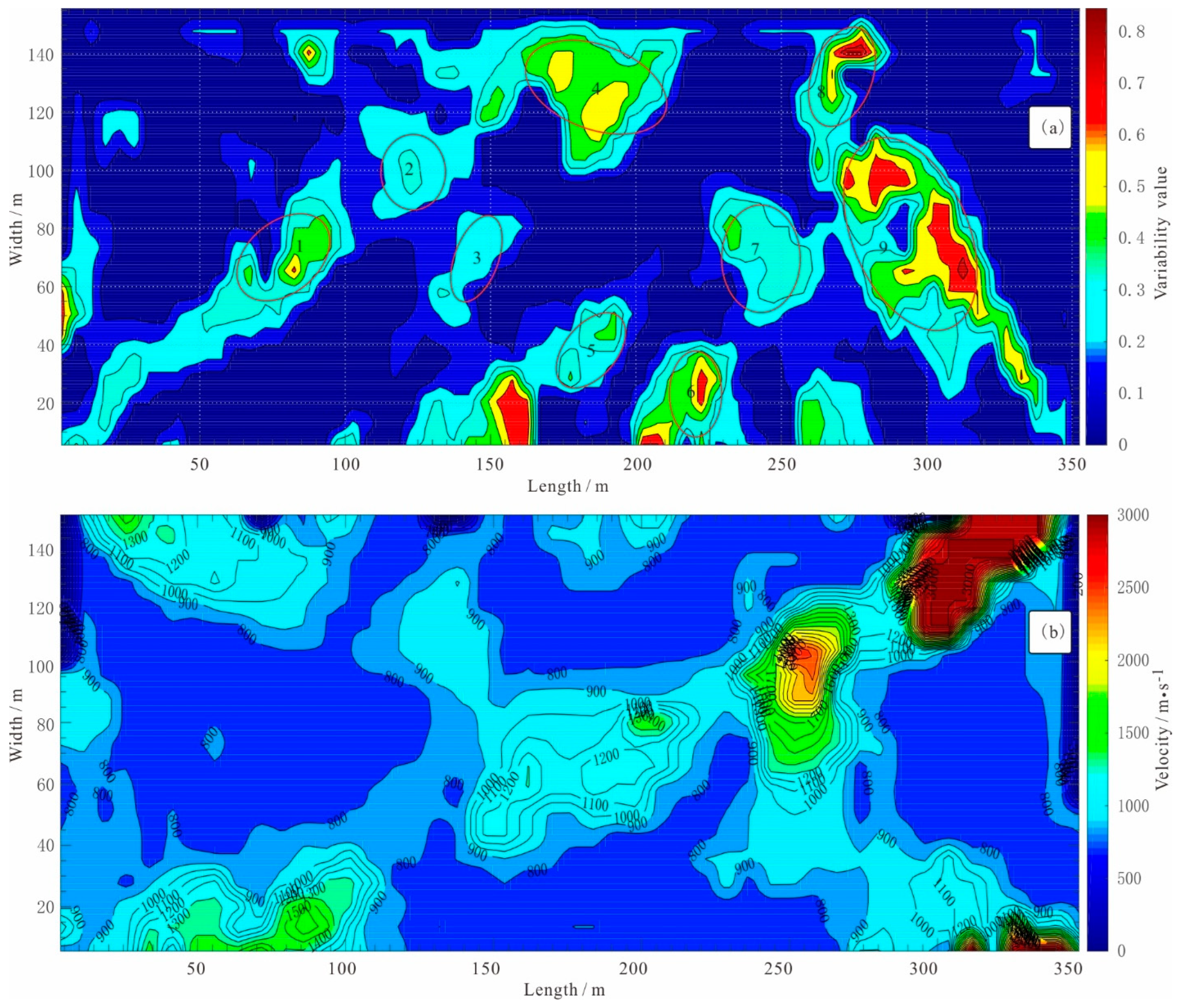
By incorporating the dispersion curve variability parameter in the table into Equation (1), the variability value (0.6842) of the channel wave in the source No. 10 and receiver No. 18 is obtained. Similarly, the variability values of all channel wave data were obtained and incorporated into Equation (3) to obtain the variability distribution in the detection area, as shown in Figure 6a, whereas Figure 6b shows the travel time imaging results.

The CT imaging results of the variability function show that there are anomalies near the positions of the collapse columns X638, X639, X640, X639, and X640 exposed in the air return roadway and the laneway of the working face, and the variability coefficient is relatively high. At the same time, nine regions of variability anomalies are revealed in the working face, with different sizes and shapes of the anomalies. From left to right, the anomaly bodies are numbered 1-9. According to geological data, all 9 anomaly bodies are interpreted as collapse columns. The mining verifies that No. 1–9 collapse columns exist. Among them, No. 1, 2, 3, 5, 6, and 8 collapse columns are small in scale, with the long axis being less than 30 m. No. 4, 7, and 9 collapse columns are large in scale, with the long axis being greater than 40 m. Among them, No. 9 collapse column has a long axis of 70 m and a short axis of 40 m. The positions of No. 7, 8, and No. 9 collapse columns are close to the DX4 positions speculated by the surface 3D seismic, and the channel wave detection results are more accurate. Collapse pillars No. 1–9 were verified by back mining with a positional deviation of less than 5 m.

During travel time tomography, the travel time or velocity information picked up generally corresponds to a fixed frequency. When picking up travel time at a fixed frequency of 125Hz, as shown in Figure 6b, the picking error is large, which affects the imaging results. The CT imaging results of velocity reveal that abnormal areas at the collapse pillars X638, X639, X640, X642, and X643 locations exposed in the working face return airways and laneway, with relatively high wave velocities (all greater than 1100 m/s), but the images are deviations from the correct positions. A number of abnormal areas with obvious high velocities were found within the working face and were errors with the verification results (Figure 6b).

It can be seen from the comparative analysis of Figure 6a,b as well as the mining verification results that the error of the variability function imaging method is small and more accurate. When the coal seam is stable, the inversion of the abnormal body is better than conventional tomography. The function construction can effectively reflect the combination characteristics of the time domain and frequency domain and carry out variance imaging through the constraint of theoretical velocity on actual and the breakpoint feature of the abnormal body, with errors being reduced and results more stable.

4. Conclusions

In this paper, based on the changes in the dispersion curve when the channel wave passes through an abnormal body, the variability imaging method is proposed. The variability is related not only to the number and type of breaking points in the dispersion curve but also to the velocity, frequency, and the corresponding spectral value of the breaking point position. Thus, the variability function imaging method has not only kinematic characteristics but also kinetic characteristics. The variability function tomography method effectively reduces the number of unknowns and improves computational efficiency. The method overcomes the disadvantage of the uncertainty of extracting travel time information in velocity tomography and quantitatively analyzes the breakpoints of the dispersion curve, which reduces the error caused by processors and makes the calculation result more stable. Through example calculations, the method is able to identify irregular collapse columns. The imaging result is more accurate to explain the location and shape of the DX4 anomaly area than the result delineated by 3D seismic, and the delineated collapse column anomaly is consistent with the recovery verification.