Article

Forecast of AMD Quantity by a Series Tank Model in Three Stages: Case Studies in Two Closed Japanese Mines

1
Faculty of Science and Engineering, Waseda University, 3-4-1 Okubo, Shinjuku-ku, Tokyo 169-8555, Japan
2
Graduate School of Creative Science and Engineering, Waseda University, 3-4-1 Okubo, Shinjuku-ku, Tokyo 169-8555, Japan
*
Author to whom correspondence should be addressed.
Minerals 2020, 10(5), 430; https://doi.org/10.3390/min10050430
Submission received: 8 April 2020 / Revised: 9 May 2020 / Accepted: 9 May 2020 / Published: 11 May 2020

Abstract

:
There are about 100 sites of acid mine drainage (AMD) from abandoned/closed mines in Japan. For their sustainable treatment, future prediction of AMD quantity is crucial. In this study, AMD quantity was predicted for two closed mines in Japan based on a series tank model in three stages. The tank model parameters were determined from the relationship between the observed AMD quantity and the inflow of rainfall and snowmelt by using the Kalman filter and particle swarm optimization methods. The Automated Meteorological Data Acquisition System (AMeDAS) data of rainfall were corrected for elevation and by the statistical daily fluctuation model. The snowmelt was estimated from the AMeDAS data of rainfall, temperature, and sunshine duration by using mass and heat balance of snow. Fitting with one year of daily data was sufficient to obtain the AMD quantity model. Future AMD quantity was predicted by the constructed model using the forecast data of rainfall and temperature proposed by the Max Planck Institute–Earth System Model (MPI–ESM), based on the Intergovernmental Panel on Climate Change (IPCC) representative concentration pathway (RCP) 2.6 and RCP8.5 scenarios. The results showed that global warming causes an increase in the quantity and fluctuation of AMD, especially for large reservoirs and residence time of AMD. There is a concern that for mines with large AMD quantities, AMD treatment will be unstable due to future global warming.

1. Introduction

Japan has more than 5000 abandoned/closed mines, and about 100 of their sites produce acid mine drainage (AMD) due to the presence of sulfide mineralization [1]. The general treatment for AMD is neutralization and sedimentation by addition of a neutralizer, such as lime, calcium carbonate, and sodium hydroxide [2], and solid/liquid separation [3] of the produced sludge from the neutralized effluents. In these treatments, all toxic elements are concentrated into the sludge by precipitation [4,5,6] and adsorption [7,8,9,10,11,12], and the sludge is controlled in a tailing pond at a mine site or final disposal site. For these last several decades, AMD has been treated properly in Japan and has not caused severe pollution. However, since our results of the statistical calculation (details are shown below) suggested that some mines have required AMD treatment for over 150 years [13,14] and other groups suggested that more than 1000 years of treatment will be necessary [15] in the current situation, more sustainable treatment to reduce both AMD generation [16,17] and treatment cost [18] is needed. To reduce the treatment cost of the addition of chemicals and of sludge generation, for example, a passive treatment that utilizes the natural environment of mines, such as topography, plants, and microorganisms, has attracted attention as a sustainable AMD treatment based on new concepts [19,20,21]. Several researchers are trying to successfully reuse this sludge as an industrial material [22,23].
Unlike industrial wastewater, AMD quantity and quality differ significantly in mines due to regional, geological, mineralogical, and biological factors. Therefore, it is necessary to customize an appropriate treatment for each mine. To select an optimal treatment method from the various treatment technologies, including those based on both active and passive concepts, an accurate understanding of the current potential for AMD generation [24,25] and the future forecast of AMD quantity and quality are essential.
The objective of this study was to determine a forecast for AMD quantity. To accomplish this, we constructed a model that reproduces the current AMD quantity using previous monitoring data of AMD, and then extrapolated it to the future. To reproduce AMD quantity, there are two ways: one is a hydraulic simulation [26,27,28,29,30,31] and the other is a tank model. A hydraulic simulation provides detailed information on the origin and distribution of AMD and can be a powerful tool for discussing AMD generation countermeasures, but it requires, in addition to meteorological data, detailed geological, mineralogical, and hydraulic data, which are generally difficult to obtain, especially for abandoned and closed mines. On the other hand, a tank model is a blackbox to determine the relationship between inflow and outflow, but just inflow data of rainfall and snowmelt and outflow of AMD quantity are sufficient for the model [32,33]. In this study, the tank model was selected for AMD quantity modeling, and rainfall and snowmelt were used as inflow. The rainfall data were corrected for elevation and adjusted using the statistical daily fluctuation model to suit each AMD site. Snowmelt was also estimated from rainfall by considering mass and heat balance by using temperature and sunshine duration data. We did not select a hydraulic simulation but chose a statistical model because our target mines are closed and it was difficult to obtain detailed monitoring, geological, and hydraulic data for this study.
For the AMD quality model, we previously reported the geochemical calculation with first-order elution kinetics of sulfide minerals [13,14]. In the model, sulfides that should be the source of AMD were selected from the quality data, and their first-order elution rate and initial AMD generation potential were estimated by fitting to the time change of their elution amount obtained from the AMD quantity and quality data. The AMD quality could be estimated by the coupling of the kinetics for sulfide elution and oxidation, and the geochemical code for the chemical equilibrium calculation of precipitation and adsorption [34,35,36,37]. This means that accurate estimation of AMD quantity is crucial for the AMD quality model.
In this study, the AMD quantity model was constructed using two case studies of underground mines: a closed sulfur mine (Mine A) and a closed black-ore copper, lead, and zinc mine (Mine B). Mine A has a large quantity of AMD, averaging 18 m3 min−1 with a small fluctuation, which is opposite to that from Mine B (1.5 m3 min−1). From these case studies, the parameters of the model were estimated and the future AMD quantity for the next few decades was predicted using forecast data for rainfall and temperature based on the MPI–SEM (Max Planck Institute–Earth System Model) [37]. For this, we selected two kinds of global warming scenarios proposed by IPCC (Intergovernmental Panel on Climate Change): a low-stabilization scenario of RCP (representative concentration pathway) 2.6 and a high-level greenhouse gas emission scenario of RCP 8.5 [37]. We further discuss the effects of global warming on the forecast of AMD quantity stemming from the closed sulfide mines that were examined.

2. Materials and Methods

2.1. AMD Quantity Model
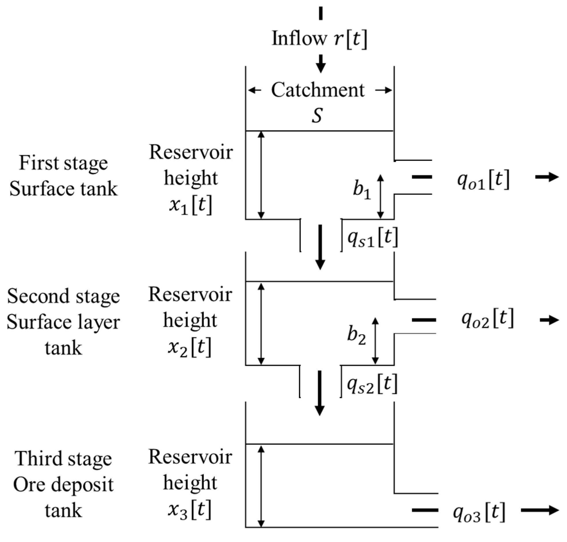
2.1.1. Tank Model

The AMD quantity model was constructed by using a series tank model in three stages, as shown in Figure 1. The first and second stages correspond to the nonpolluted water reservoir on the surface and inside the mine, respectively. The third stage corresponds to the polluted water reservoir in the ore deposit that causes AMD. Inflow, r (mm), is the summation of rainfall, rw, and snowmelt, rs. In each tank, a part of the inflow is distributed to the outflow (mm h−1), qoi (i = 1, 2, 3), and seepage flow to the next tank, qsi (i = 1, 2), according to the water reservoir height (mm), xi (i = 1, 2, 3) and outflow height (mm), bi (i = 1, 2). The water balance in each tank is as follows:
dxi/dt = qsi–1qsiqoi, (i = 1, 2, 3)
where t is time, qs0 = r = rw + rs, and qs3 = 0. The outflow is calculated from:
qoi = aoi (xibi), (i = 1, 2, 3)
where aoi (i = 1, 2, 3) is the outflow coefficient and b3 = 0. The seepage flow is also calculated from:
qsi = asi xi, (i = 1, 2)
where asi (i = 1, 2) is the seepage coefficient.
In this study, qo3 corresponded to AMD quantity. The inflow, r, was set using the following procedure. The Kalman filter and particle swarm optimization methods were used for fitting qo3 to the observed data of AMD quantity to estimate the xi, bi, asi, and aoi parameters [38].

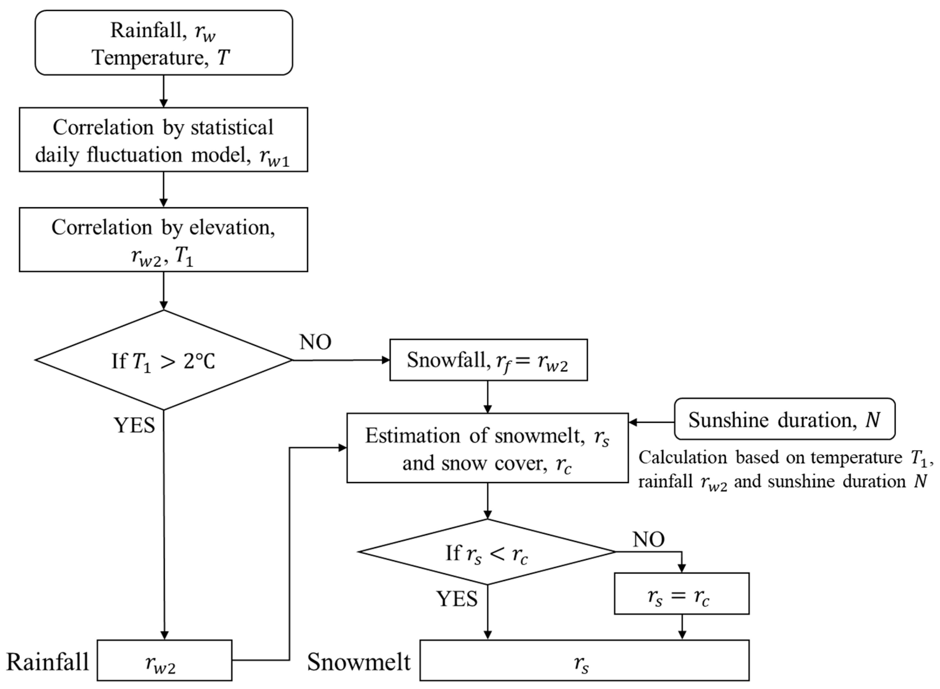
2.1.2. Correction of Rainfall Data and Judgment of Snowfall

Rainfall data near each mine were derived from AMeDAS (Automated Meteorological Data Acquisition System) provided by the Japan Meteorological Agency [39]. To suit each mine situation, the daily data of rainfall and temperature obtained from AMeDAS were corrected for elevation and adjusted by using the statistical daily fluctuation model, as shown in Figure 2. Also, snowfall was estimated according to the corrected temperature, and if the temperature was under 2 °C, it was judged to be snowfall and not rainfall.
Since the capture rate of rainfall particles by the rain gauge decreases as the wind speed increases, known as the Jebons effect, Kondo et al. proposed the following statistical correction for daily rainfall data obtained from AMeDAS [40]:
rw1 = (1.25 + 0.15 cos(w(d − 20)))rw0
w = 2π/365
where rw0 (mm) is the raw rainfall data, rw1 (mm) is the corrected rainfall data by the model, d (days) refers to the days from 1 January. Furthermore, the amount of rainfall near mines depends greatly on elevation due to rapid updraft and adiabatic expansion, and is corrected as follows [40]:
rw2 = (1 + c(hh0))rw1
where rw2 (mm) is the corrected rainfall data by elevation, h (km) is the elevation of mine site, h0 (km) is the elevation of the AMeDAS observation point, and c is the coefficient (0.001 km−1 for 5 °C or less and 0.00064 km−1 for 5 °C or more). AMeDAS data of temperature, T, were also corrected according to following equation:
T1 = −6(hh0) + T
where T1 (°C) is the corrected temperature.
As shown in Figure 2, if the temperature at the mine site was above 2 °C, it was assumed that there was no snowfall and the inflow of rainfall was set as rw2. On the other hand, if the temperature was below 2 °C, the rainfall data, rw2, were judged to be equivalent to snowfall, rf = rw2, and rw2 = 0.

2.1.3. Estimation of Snowmelt and Snow Cover

Daily snowmelt, rs, and snow cover, rc, were also estimated by following the mass and heat balance of snow using the AMeDAS data of rainfall, temperature, and sunshine duration, as shown in Figure 2. If the temperature was below 0 °C, no snowmelt was assumed and rs = 0; otherwise, snowmelt was calculated according to the following procedure.
Snowmelt, rs (mm), was calculated from the ratio of fusion heat, Q (J), and latent heat, L (334 J kg−1), the catchment area, S (mm2), and the density of water, ρ (9.97 × 10⁻⁷ kg mm−3):
rsSρ = Q/L
The fusion heat was calculated from the heat balance of snow exposure as follows:
Q = Q1 + Q2 + Q3 + Q4 + Q5
where Q1 is the short-wavelength radiation, Q2 is the long-wavelength radiation, Q3 is the sensible heat transfer, Q4 is the latent heat transfer, and Q5 is the transfer heat due to rainfall. Here, heat changes in the snow layer and heat transfer from the ground were assumed to be negligible [41].
The short-wavelength radiation was calculated from albedo, r, which is the ratio of reflected sunshine radiation to sunshine radiation on the earth’s surface and the daily average of solar irradiance, I (W m−2):
Q1 = (1 − r)I
The average of solar irradiance was the function of the ratio of sunshine duration, N, and astronomical sunshine duration, N0 [42]:
I/I0 = 0.179 + 0.550N/N0, for 0 ≤ NN0
I/I0 = 0.114, for N = 0
where I0 is the solar irradiance at the top of atmosphere. The values of solar irradiance at the top of the atmosphere, I0, astronomical sunshine duration, N0, and albedo, r, are available from references [39,43], and sunshine duration data, N, are available from AMeDAS.
The long-wavelength radiation was the difference between the radiation from the atmosphere, Qa, and the radiation from the snow surface, Qs:
Q2 = QaQs
Qa = σ(T1 + 273.15)4(0.605 + 0.048e0.5)
Qs = 0.9σ(Ts + 273.15)4
e = 6.1078 × 107.5T/(T+273.3)
where σ is the Stefan–Boltzmann constant (5.67 × 10⁻⁸ W m−2 K−4) and e is amount of saturated water vapor [44]. The temperature of the snow surface, Ts, was calculated from [45]:
Ts = 1.13T1 − 1.67
when T1 ≤ 1.47.
The sensible heat was calculated from [46]:
Q3 = K(1 − 0.0065h/(T1 + 273.15+0.0065h))5.257, for T1 ≥ 0,
Q3 = 0, for T1 ≤ 0
where K is the transfer coefficient of the sensible heat and the latent heat; 3.5 was proposed for the area near the mines that were modeled in this case study [46]. The latent heat was calculated from:
Q4 = 1.53K(e − 6.11), for T1 ≥ 7
Q4 = 0, for T1 ≤ 7
The transfer heat due to rainfall was calculated from:
Q5 = ρcw(273.15 + T1)rwS
where cw is the specific heat of the water (4.186 J kg−1 K−1).
The snowmelt, rs, calculated from Equations (8) to (22), should be less than the snow cover, rc. Snow cover was calculated from following summation of daily mass balance:
rc = ∑rf − ∑rs
if rs > rc, then snowmelt should be rs = rc.

2.2. Forecast Data of Temperature, Rainfall, and Sunshine Duration

In the above-mentioned AMD quantity and quality models, daily data of rainfall, average temperature, and sunshine duration obtained from AMeDAS were used for model construction. Therefore, future forecasts of daily data of rainfall, average temperature, and sunshine duration were also necessary for the forecast of AMD quantity and quality in the future. For the AMD quality model, the geochemical calculation with first-order elution kinetics of sulfide minerals was used as mentioned above; the first-order elution rate and initial AMD generation potential were estimated by fitting to the time change of their elution amount obtained from the AMD quantity and quality data. The daily output data of MPI–ESM (Max Planck Institute–Earth System Model), which is an earth system model proposed by Max Planck Institute, were used in this study. Two kinds of IPCC RCPs for the greenhouse gas (GHG) concentration scenario were selected: RCP2.6 and RCP8.5. The former is the scenario with the lowest GHG emission to keep future temperature rise below 2 °C, and the latter is the scenario with the highest GHG emissions.
From the system, daily forecast data of rainfall, average temperature, and maximum and minimum temperatures were available. The daily forecast of the average of solar irradiance, I, was estimated from [47]:
I = 0.76I0(1− exp(−AΔT2.2))
A = 0.036exp(−0.154ΔTave)
where ΔT is the difference between the maximum temperature and the minimum temperature, and ΔTave is the monthly average of ΔT.

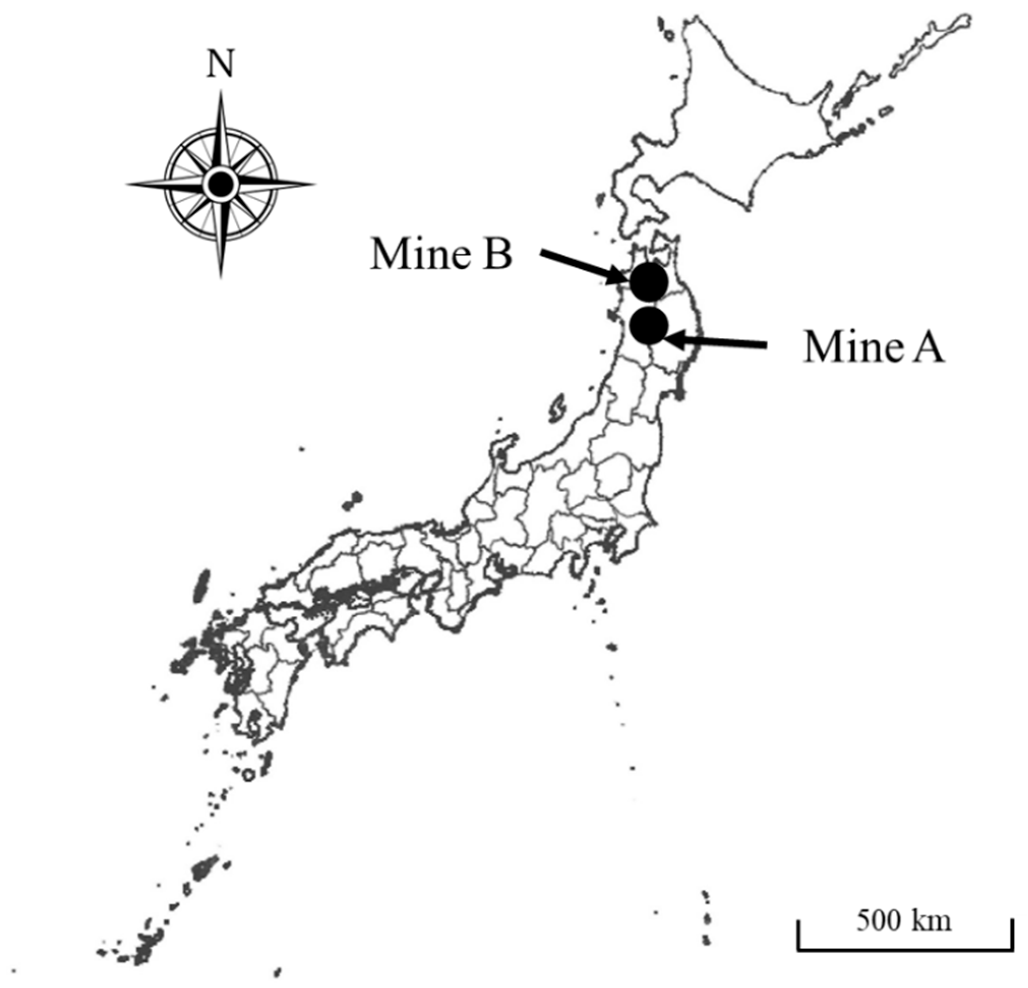
2.3. Case Studies in Two Closed Mines

In this study, two closed underground mines in the northern part of Japan were selected as a case study; Mine A has a large quantity of AMD, with small fluctuation of quantity and quality, and Mine B has a small quantity of AMD, with large fluctuation of quantity and quality. Snow is observed in winter at both of the closed mines. The locations of the mines are shown in Figure 3, and the AMD characteristics are shown in Table 1.
In Mine A, native sulfur and pyrite were mined during its operation. The size of the ore deposit was about 1500 m East–West, about 1500 m North–South, and 25–150 m of thickness, and ore reserves were about 230 million tons per year. The mine produced about 1 million tons of ore and one-third of Japan’s sulfur demand, but it closed in 1971 due to the market influence of sulfur recovered from oil refining. The quantity of AMD is about 18 m3 min−1 on average annually, which is one of the largest AMD values in Japan [48]. The AMeDAS point is located 11 km east and 825 m below the mine.
In Mine B, copper, lead, and zinc were mined during its operation. The ore deposit was a black ore type, which has changed from lower to yellow ore, black ore, and quartz band. The mine produced a maximum of about 25,000 tons per year, but closed in 1985 due to ore depletion. The annual average of the AMD quantity was 1.72 m³ min−1 in 2017 and increased from 5 to 7 m³ min−1 during the snowmelt season [49]. The AMeDAS point is located 18 km northwest and 465 m below the mine.

3. Results and Discussion

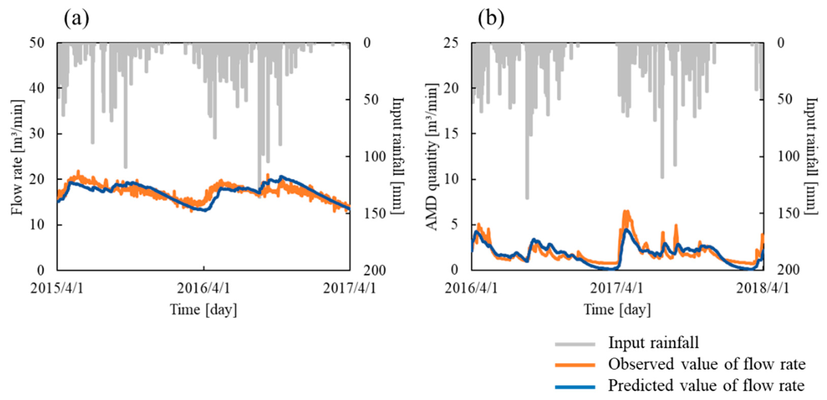
3.1. AMD Quantity Model Construction

The relation between the input data of AMeDAS rainfall (upper side) and the observed data and the calculated value of AMD quantity (underside) are shown in Figure 4. In this calculation, the daily observed data of AMD quantity in the prior one year were used for fitting, and later one-year data were used for the model validation. The fitting period was also changed from half a year to two years and the correlation coefficients between the observed and calculated values were compared, as shown in Table 2 and Supplementary Figure S1. Of course, the longer the fitting period, the higher the correlation coefficient in the validation period, but a fitting period of one year seemed to be generally sufficient for the reproduction of AMD quantity in the next one year. As shown in Supplementary Figure S2, when the correction for elevation and the statistical daily fluctuation and the snowmelt estimation were not conducted, the reproducibility of AMD quantity became worse, especially for Mine A. This is because Mine A is located at a higher elevation and the effects of elevation correction and snowfall are larger than for Mine B.
The parameters obtained for the tank model are shown in Table 3. Mine A has a smaller outflow height and a larger AMD reservoir than Mine B. Additionally, Mine A has the smaller value of outflow coefficient in the third stage, which directly affects AMD generation, compared to Mine B. This trend means that Mine A has the bigger reservoir and the longer residence time of AMD, which resulted in the smaller fluctuation of AMD, compared to Mine B. As we mentioned in the previous section, ore production was 230 million tons per year in Mine A and 25,000 tons per year in Mine B. This difference in scale should directly affect the difference in reservoir and residence time of AMD.

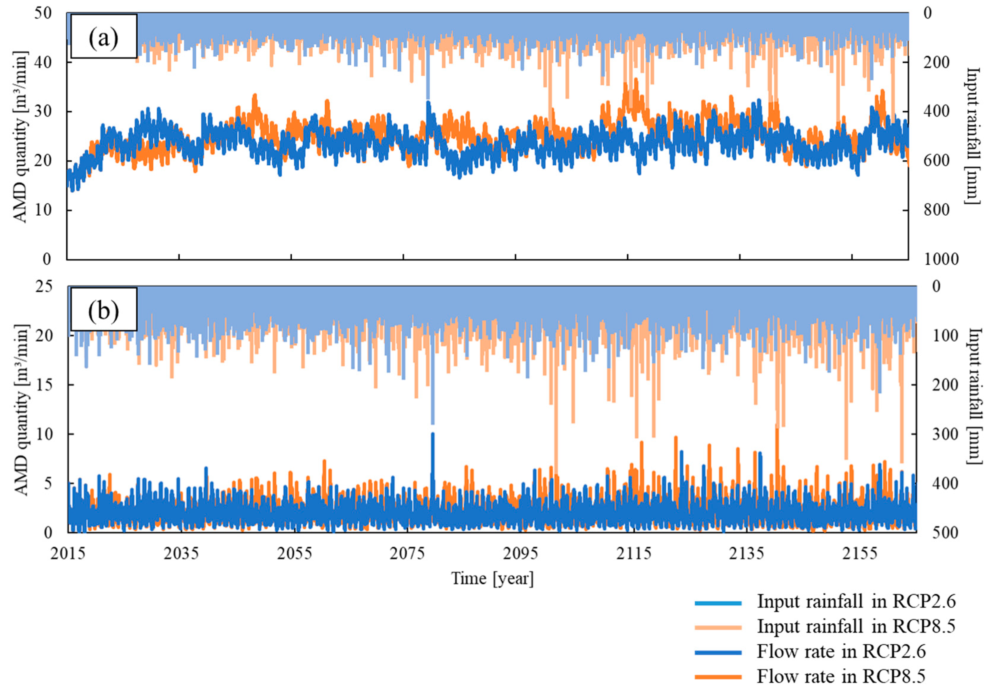
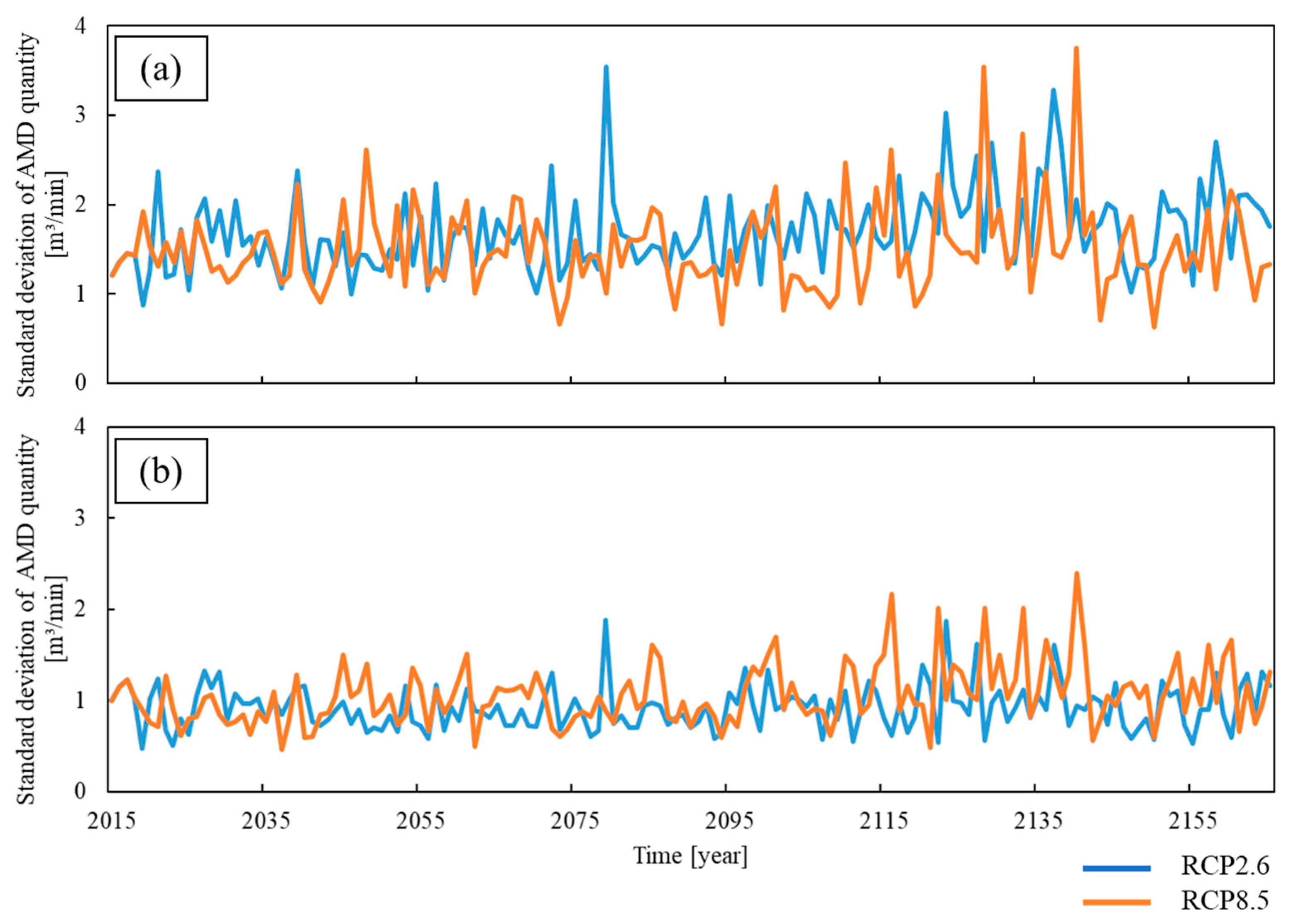
3.2. Forecast of AMD Quantity

The forecast of AMD quantity (underside) is shown in Figure 5, with the forecast of rainfall (upperside) proposed by MPI–ESM. According to MPI–ESM in RCP2.6, the forecast for temperature rise around the mines is about 2 °C by 2050, but remaining at about 1.0–2.5 °C after 2050. On the other hand, in RCP8.5, the forecast for temperature continues to rise and reaches +5.9 °C in 2100.
In Mine A, the MPI–ESM shows that both rainfall and heavy rain frequency, which is the number of days per year with greater than 50 mm of rainfall, increase due to the temperature rise. In 2100, the forecast of rainfall is +21% for both RCP2.6 and RCP8.5, and forecast of heavy rain frequency increases 4 days/year for RCP2.6 and 8 days/year for RCP8.5, compared to the present. According to these trends, the AMD quantity calculated from the constructed model increases, as shown in Figure 5. The forecast for AMD quantity in 2100 is +27% for RCP2.6 and +31% for RCP8.5.
In Mine B, the MPI–ESM shows that the temperature rise of around 2 °C in the RCP2.6 scenario does not have much effect on rainfall and heavy rain frequency. In 2100, the forecast for rainfall decreases 1.5% and heavy rain frequency decreases 2 days/year, which results in a 0.55% increase for the forecast of AMD quantity, compared to the present. However, the temperature rise of 5.9 °C in the RCP8.5 scenario affects the forecast of rainfall and heavy rain frequency as much as for Mine A. In 2100, the rainfall forecast increases 22% and heavy rain frequency increases 5.5 days/year, which results in a 25% increase for the forecast of AMD quantity, compared to the present.
The forecast of the standard deviation of AMD quantity is shown in Figure 6. A comparison of the coefficient of variation of AMD quantity between the present and the future is shown in Table 4. Here, the coefficient of variation was calculated for 10 years from 2010 to 2020 for the present and from 2100 to 2110 for the future. The temperature rise due to global warming caused larger fluctuations in the AMD quantity for Mine A. In the case of Mine B, since the AMD reservoir is small and the AMD residence time is short, even if the rainfall fluctuation increases in the future due to global warming, the AMD fluctuation will remain largely as it is now. On the other hand, in the case of Mine A, since the AMD reservoir is larger and the AMD residence time is longer, AMD fluctuation tends to increase gradually in the future, affected by increases in rainfall fluctuation due to global warming. This trend suggests that AMD treatment might be unstable because of global warming in the future, especially for mines with larger AMD quantities.
In general, AMD quality tends to deteriorate as the AMD quantity increases. This is because when the AMD quantity increases, AMD comes in contact with a new pollution source in the mine. Actually, at present, the fluctuation of AMD quantity is larger in Mine B than in Mine A, and the fluctuation in AMD quality tends to be larger in Mine B as well. This suggests that fluctuations in AMD quantity due to global warming will cause large fluctuations in AMD quality.

4. Conclusions

The AMD quantity model was constructed for two closed mines in Japan. The model was constructed with a series tank model, and fitted by using daily data for one year, which were enough to obtain adequate parameters. The results showed that Mine B has a smaller AMD reservoir and a shorter AMD residence time than Mine A, resulting in a large fluctuation of AMD quantity in Mine B. The forecast of AMD quantity was also estimated based on the forecast of rainfall and temperature proposed by the MPI–ESM with IPCC RCP2.6 and RCP8.5 scenarios. The forecast results showed that temperature rise due to global warming will cause an increase in rainfall, resulting in increased AMD quantity. The fluctuation of rainfall will also increase due to global warming, increasing the fluctuation of AMD quantity in Mine A. The effect of global warming in Mine A will be bigger than in Mine B due to its larger reservoir and longer residence time of AMD.
In this study, it is expected that the quantity and fluctuation of AMD might increase due to global warming. This suggests that fluctuations in AMD quality might also increase. Therefore, when selecting future treatment methods, careful consideration should be given to whether or not the AMD fluctuation can be sufficiently dealt with in the future, especially for passive treatment.

Supplementary Materials

The following are available online at https://www.mdpi.com/2075-163X/10/5/430/s1, Figure S1: Observed and calculated AMD quantity by the tank model for (a) Mine A with half-year fitting, (b) Mine A with two-year fitting, (c) Mine B with half-year fitting, and (d) Mine B with two-year fitting; Figure S2: Observed and calculated AMD quantity by the tank model without correction of rainfall and temperature or considering snowmelt for (a) Mine A and (b) Mine B.

Author Contributions

Conceptualization, C.T.; methodology, K.F.; validation, M.K. and S.F.; investigation, K.F.; data curation, S.F.; writing—original draft preparation, C.T.; writing—review and editing, K.F. and S.F.; supervision, C.T. All authors have read and agreed to the published version of the manuscript.

Funding

This research was partially funded by JOGMEC (Japan Oil, Gas and Metals National Corporation) and the Center for Eco-Mining, Japan.

Acknowledgments

Part of this work was performed as the activities of the Waseda Research Institute for Science and Engineering and Research Organization for Open Innovation Strategy, Waseda University.

Conflicts of Interest

The authors declare no conflict of interest.

References

  1. JOGMEC (Japan Oil, Gas and Metals National Corporation). Mine Pollution Control. Available online: http://www.jogmec.go.jp/english/mp_control/index.html (accessed on 22 March 2020).
  2. Tokoro, C. Removal mechanism in anionic co-precipitation with hydroxides in acid mine drainage treatment. Resour. Process. 2015, 62, 3–9. [Google Scholar] [CrossRef] [Green Version]
  3. Tokoro, C. As (V) removal by Fe (III), Al or Pb salts and rapid solid/liquid separation in wastewater containing dilute arsenic—A fundamental study for efficient treatment of wastewater containing dilute arsenic (Part 1). J. Mmij. 2005, 121, 399–406. [Google Scholar] [CrossRef]
  4. Onoguchi, A.; Granata, G.; Haraguchi, D.; Hayashi, H.; Tokoro, C. Kinetics and mechanism of selenate and selenite removal in solution by green rust-sulfate. R. Soc. Open Sci. 2019, 6, 182147. [Google Scholar] [CrossRef] [PubMed] [Green Version]
  5. Mamun, A.; Onoguchi, A.; Granata, G.; Tokoro, C. Role of pH in green rust preparation and chromate removal from water. Appl. Clay Sci. 2018, 165, 205–213. [Google Scholar] [CrossRef]
  6. Tokoro, C.; Suzuki, S.; Haraguchi, D.; Izawa, S. Silicate removal in aluminum hydroxide co-precipitation process. Materials 2014, 7, 1084–1096. [Google Scholar] [CrossRef] [PubMed]
  7. Tokoro, C.; Kadokura, M.; Kato, T. Mechanism of arsenate coprecipitation at the solid/liquid interface of ferrihydrite: A perspective review. Adv. Powder Technol. 2020, 31, 859–866. [Google Scholar] [CrossRef]
  8. Mamun, A.; Morita, M.; Matsuoka, M.; Tokoro, C. Sorption mechanisms of chromate with coprecipitated ferrihydrite in aqueous solution. J. Hazard. Mater. 2017, 334, 142–149. [Google Scholar] [CrossRef]
  9. Haraguchi, D.; Tokoro, C.; Oda, Y.; Owada, S. Sorption mechanisms of arsenate in aqueous solution during coprecipitation with aluminum hydroxide. J. Chem. Eng. Jpn. 2012, 46, 173–180. [Google Scholar] [CrossRef]
  10. Tokoro, C.; Koga, H.; Oda, Y.; Owada, S.; Takahashi, Y. XAFS investigation for As (V) co-precipitation mechanism with ferrihydrite. J. Mmij. 2011, 127, 213–218. [Google Scholar] [CrossRef] [Green Version]
  11. Tokoro, C.; Yatsugi, Y.; Koga, H.; Owada, S. Sorption mechanisms of arsenate during coprecipitation with ferrihydrite in aqueous solution. Environ. Sci. Technol. 2010, 44, 638–643. [Google Scholar] [CrossRef]
  12. Sasaki, K.; Qiu, X.; Moriyama, S.; Tokoro, C.; Ideta, K.; Miyawaki, J. Characteristic sorption of H3BO3/B (OH)4−on magnesium oxide. Mater. Trans. 2013, 54, 1809–1817. [Google Scholar] [CrossRef] [Green Version]
  13. Koide, R.; Tokoro, C.; Murakami, S.; Adachi, T.; Takahashi, A. A model for prediction of neutralizer usage and sludge generation in the treatment of acid mine drainage from abandoned mines: Case studies in Japan. Mine Water Environ. 2012, 31, 287–296. [Google Scholar] [CrossRef]
  14. Otsuka, H.; Murakami, S.; Yamatomi, J.; Koide, R.; Tokoro, C. A predictive model for the future treatment of acid mine drainage with regression analysis and geochemical modeling. J. Mmij. 2014, 130, 488–493. [Google Scholar] [CrossRef] [Green Version]
  15. Tabelin, C.; Sasaki, A.; Igarashi, T.; Tomiyama, S.; Tabelin, M.V.; Ito, M.; Hiroyoshi, N. Prediction of acid mine drainage formation and zinc migration in the tailings dam of a closed mine, and possible countermeasures. Matec. Web Conf. 2019, 268, 06003. [Google Scholar] [CrossRef]
  16. Ogbughalu, O.T.; Gerson, A.R.; Qian, G.; Smart, R.S.C.; Schumann, R.C.; Kawashima, N.; Fan, R.; Li, J.; Short, M.D. Heterotrophic microbial stimulation through biosolids addition for enhanced acid mine drainage control. Minerals 2017, 7, 105. [Google Scholar] [CrossRef] [Green Version]
  17. Qian, G.; Schumann, R.C.; Li, J.; Short, M.D.; Fan, R.; Li, Y.; Kawashima, N.; Zhou, Y.; Smart, R.S.C.; Gerson, A.R. Strategies for reduced acid and metalliferous drainage by pyrite surface passivation. Minerals 2017, 7, 42. [Google Scholar] [CrossRef]
  18. Nguyen, H.T.H.; Nguyen, B.Q.; Duong, T.T.; Bui, A.T.K.; Nguyen, H.T.A.; Cao, H.T.; Mai, N.T.; Nguyen, K.M.; Pham, T.T.; Kim, K.-W. Pilot-scale removal of arsenic and heavy metals from mining wastewater using adsorption combined with constructed wetland. Minerals 2019, 9, 379. [Google Scholar] [CrossRef] [Green Version]
  19. Kato, T.; Fukushima, R.; Granana, G.; Sato, K.; Yamagata, S.; Tokoro, C. Quantitative modeling incorporating surface complexation for zinc removal using leaf mold. J. Soc. Powder Technol. Jpn. 2019, 56, 136–141. [Google Scholar] [CrossRef]
  20. Lefticariu, L.; Behum, P.T.; Bender, K.S.; Lefticariu, M. Sulfur Isotope fractionation as an indicator of biogeochemical processes in an AMD passive bioremediation system. Minerals 2017, 7, 41. [Google Scholar] [CrossRef] [Green Version]
  21. Johnson, D.B. Recent developments in microbiological approaches for securing mine wastes and for recovering metals from mine waters. Minerals 2014, 4, 279–292. [Google Scholar] [CrossRef]
  22. Herrera, P.S.; Uchiyama, H.; Igarashi, T.; Asakura, K.; Ochi, Y.; Ishizuka, F.; Kawada, S. Acid mine drainage treatment through a two-step neutralization ferrite-formation process in northern Japan: Physical and chemical characterization of the sludge. J. Miner. Eng. 2007, 20, 1309–1314. [Google Scholar] [CrossRef]
  23. Igarashi, T.; Herrera, P.S.; Uchiyama, H.; Miyamae, H.; Iyatomi, N.; Hashimoto, K.; Tabelin, C.B. The two-step neutralization ferrite-formation process for sustainable acid mine drainage treatment: Removal of copper, zinc and arsenic, and the influence of coexisting ions on ferritization. Sci. Total Environ. 2020, 715, 136877. [Google Scholar] [CrossRef]
  24. Matsumoto, S.; Ishimatsu, H.; Shimada, H.; Sasaoka, T.; Kusuma, G.J. Characterization of mine waste and acid mine drainage prediction by simple testing methods in terms of the effects of sulfate-sulfur and carbonate minerals. Minerals 2018, 8, 403. [Google Scholar] [CrossRef] [Green Version]
  25. Chopard, A.; Marion, P.; Mermillod-Blondin, R.; Plante, B.; Benzaazoua, M. Environmental impact of mine exploitation: An early predictive methodology based on ore mineralogy and contaminant speciation. Minerals 2019, 9, 397. [Google Scholar] [CrossRef] [Green Version]
  26. Kitamura, A.; Kurikami, H.; Sakuma, K.; Malins, A.; Okumura, M.; Machida, M.; Mori, K.; Tada, K.; Tawara, Y.; Kobayashi, T.; et al. Redistribution and export of contaminated sediment within eastern Fukushima Prefecture due to typhoon flooding. Earth Surf. Process Landf. 2016, 41, 1708–1726. [Google Scholar] [CrossRef]
  27. Sakuma, K.; Kitamura, A.; Malins, A.; Kurikami, H.; Machida, M.; Mori, K.; Tada, K.; Kobayashi, T.; Tawara, Y.; Tosaka, H. Characteristics of radio-cesium transport and discharge between different basins near to the Fukushima Dai-ichi Nuclear Power Plant after heavy rainfall events. J. Environ. Radioact. 2017, 169–170, 137–150. [Google Scholar] [CrossRef]
  28. Sakuma, K.; Malins, A.; Funaki, H.; Kurikami, H.; Niizato, T.; Nakanishi, T.; Mori, K.; Tada, K.; Kobayashi, T.; Kitamura, A.; et al. Evaluation of sediment and 137Cs redistribution in the Oginosawa River catchment near the Fukushima Dai-ichi Nuclear Power Plant using integrated watershed modeling. J. Environ. Radioact. 2018, 182, 44–51. [Google Scholar] [CrossRef]
  29. Tomiyama, S.; Igarashi, T.; Tabelin, C.B.; Tangviroon, P.; Ii, H. Modeling of the groundwater flow system in excavated areas of an abandoned mine. J. Contam. Hydrol. 2020, 230, 103617. [Google Scholar] [CrossRef]
  30. Tomiyama, S.; Igarashi, T.; Tabelin, C.B.; Tangviroon, P.; Ii, H. Acid mine drainage sources and hydrogeochemistry at the Yatani mine, Yamagata, Japan: A geochemical and isotopic study. J. Contam. Hydrol. 2020, 225, 103502. [Google Scholar] [CrossRef]
  31. Kato, T.; Kawasaki, Y.; Kadokura, M.; Suzuki, K.; Tawara, Y.; Ohara, Y.; Tokoro, C. Quantitative modeling of arsenic removal by ferrihydrite coprecipitation in an artificial wetland and pond for chemical reactions coupled GETFLOWS. Minerals 2020. under second review. [Google Scholar]
  32. Ahmad, S.W. Tank Model Application for runoff and infiltration analysis on sub-watersheds in Lalindu River in South East Sulawesi Indonesia. J. Phys. Conf. Ser. 2017, 846, 012019. [Google Scholar] [CrossRef] [Green Version]
  33. Aqili, S.W.; Hong, N.; Hama, T.; Suenaga, Y.; Kawagoshi, Y. Application of modified tank model to simulate groundwater level fluctuations in Kabul Basin, Afghanistan. J. Water Enrivon. Technol. 2016, 14, 57–66. [Google Scholar] [CrossRef] [Green Version]
  34. Tokoro, C.; Sakakibara, T.; Suzuki, S. Mechanism investigation and surface complexation modeling of zinc sorption on aluminum hydroxide in adsorption/coprecipitation processes. Chem. Eng. J. 2015, 279, 86–92. [Google Scholar] [CrossRef]
  35. Tokoro, C.; Yatsugi, Y.; Sasaki, H.; Owada, S. A quantitative modeling of co-precipitation phenomena in wastewater containing dilute anions with ferrihydrite using a surface complexation model. Resour. Process. 2008, 55, 3–8. [Google Scholar] [CrossRef]
  36. Tokoro, C.; Maruyama, Y.; Badulis, G.C.; Sasaki, H. Application of surface complexation model for dilute As removal in wastewater by Fe (III) or Al (III) salts—A fundamental study for efficient treatment of wastewater containing dilute arsenic (Part 2). J. Mmij. 2005, 121, 532–537. [Google Scholar] [CrossRef]
  37. Giorgetta, M.A.; Jungclaus, J.; Reick, C.H.; Legutke, S.; Bader, J.; Böttinger, M.; Brovkin, V.; Crueger, T.; Esch, M.; Fieg, K.; et al. Climate and carbon cycle changes from 1850 to 2100 in MPI-ESM simulations for the Coupled Model Intercomparison Project phase 5. J. Adv. Model. Earth Syst. 2013, 5, 572–597. [Google Scholar] [CrossRef]
  38. Tada, T. Parameter optimization of hydrological model using the PSO algorithm. J. Jpn. Soc. Hydrol. Water Resour. 2007, 20, 450–461. [Google Scholar] [CrossRef] [Green Version]
  39. Japan Meteorological Agency. Previous Meteorological Data and Download. Available online: https://www.data.jma.go.jp/gmd/risk/obsdl/index.php (accessed on 22 March 2020).
  40. Kondo, J.; Motoya, K.; Matsushima, D. A study on annual variations of the soil water content and water equivalent of snow in a watershed, runoff and the river water temperature by use of the new bucket-model. Meteorol. Soc. Jpn. 1995, 42, 821–831. [Google Scholar]
  41. Kurihara, J.; Yamakoshi, T.; Irasawa, M.; Sasahara, K.; Takahashi, M.; Yoshida, M. Study on the applicability of the simplified snowmelt prediction method to the Imokawa river basin, Niigata prefecture, Japan. Int. J. Eros. Control Eng. 2007, 59, 47–54. [Google Scholar]
  42. Kondo, J.; Xu, J.; Haginoya, S. Empirical formula for estimating the solar radiation at an upland from the sunshine duration data. J. Jpn. Soc. Hydrol Water Resour. 1996, 9, 468–472. [Google Scholar] [CrossRef] [Green Version]
  43. Yamazaki, T.; Kondo, J.; Taguchi, B. Estimation of the heat balance in small snowcovered forested catchment basin. Tenki 1994, 41, 71–77. [Google Scholar]
  44. Hiramatsu, S.; Irasawa, M.; Hongo, K. Study on occurrence of hillside landsides caused by snowmelt. Int. J. Eros. Control Eng. 1998, 51, 27–34. [Google Scholar]
  45. Hashimoto, T.; Ohta, T.; Ishibashi, H. Estimation of the effects of deciduous forest to the surface snowmelt by a heat balance analysis. J. Jpn. Soc. Snow Ice 1992, 54, 131–143. [Google Scholar] [CrossRef] [Green Version]
  46. Suizu, S. A snowmelt and water equivalent snow model applicable to an extensive area. J. Jpn. Soc. Snow Ice 2002, 64, 617–630. [Google Scholar] [CrossRef]
  47. Shinohara, Y.; Komatsu, H.; Otsuki, K. A method for estimating global solar radiation from daily maximum and minimum temperatures: Its applicability to Japan. J. Jpn. Soc. Hydrol Water Resour. 2007, 20, 462–469. [Google Scholar] [CrossRef]
  48. Fujii, N. On the wastewater processing plant at the closed Matsuo Mine. J. Clay Sci. Soc. Jpn. 1994, 34, 184–186. [Google Scholar]
  49. Asami, Y.; Nishida, Y.; Kimura, H.; Iwasawa, M. Nurukawa Kozan no tankokaihatsu oyobi sonogo no sogyo jokyo. J. Mininig Metall. Inst. Jpn. 1988, 104, 185–190. (In Japanese) [Google Scholar]
Figure 1. Schematic of the tank model in three stages used for the acid mine drainage (AMD) quantity model in this study.
Minerals 10 00430 g001
Figure 2. Procedural flow to obtain the inflow for the tank model (rainfall and snowmelt) from the Automated Meteorological Data Acquisition System (AMeDAS) data of rainfall, temperature, and sunshine duration.
Minerals 10 00430 g002
Figure 3. Location of the two closed mines for case study.
Minerals 10 00430 g003
Figure 4. Observed and calculated AMD quantity by the tank model for (a) Mine A and (b) Mine B.
Minerals 10 00430 g004
Figure 5. Forecast of AMD quantity calculated from the model until 2165, with the forecast of rainfall proposed by the Max Planck Institute–Earth System Model (MPI–ESM) for (a) Mine A and (b) Mine B.
Minerals 10 00430 g005
Figure 6. Forecast of the standard deviation of AMD quantity for (a) Mine A and (b) Mine B.
Minerals 10 00430 g006
Table 1. The AMD characteristics of Mine A and B.
ItemsMine AMine BEffluent
April 1982March 2017April 1972March 2017Standard
pH2.02.33.24.75.8–8.6
Fe547 mg L−1178 mg L−1N.D.N.D.10 mg L−1
As3.3 mg L−10.93 mg L−1N.D.N.D.0.01 mg L−1
CdN.D.N.D.0.360 mg L−10.024 mg L−10.03 mg L−1
ZnN.D.N.D.90.4 mg L−114.9 mg L−12.0 mg L−1
PbN.D.N.D.0.700 mg L−10.117 mg L−10.1 mg L−1
Q17.6 m3/min14.8 m3 min−12.50 m3 min−10.77 m3 min−1
N.D.: Not detected; Q: Quantity.
Table 2. Relationship between the fitting period and the correlation coefficients.
MineFitting PeriodCorrelation Coefficient in the Fitting PeriodCorrelation Coefficient in the Validation Period 7
AHalf-year 1 0.890.65
One year 20.810.69
Two years 30.800.67
BHalf-year 4 0.860.77
One year 50.860.83
Two years 60.870.85
1 2015/10/1–2016/3/31; 2 2015/4/1–2016/3/31; 3 2014/4/1–2016/3/31; 4 2016/10/1–2017/4/1; 5 2016/4/1–2017/3/31; 6 2015/4/1–2017/3/1; 7 2016/4/1–2017/3/31 for Mine A; 2017/4/1–2018/3/31 for Mine B.
Table 3. Parameters of the tank model obtained for Mines A and B.
MineTank StageOutflow Coefficient ao (day−1)Seepage Coefficient as (day−1)Outflow Height b (mm)
AFirst stage 0.7680.5680.00484
Second stage0.9360.3520.00140
Third stage0.00282
BFirst stage0.7380.8630.0358
Second stage0.2920.6070.0205
Third stage0.0500
Table 4. The coefficient of variation for AMD quantity at present and in the future.
Mine NamePresentFuture
Mine A0.083RCP2.6: 0.092
RCP8.5: 0.090
Mine B0.56RCP2.6: 0.49
RCP8.5: 0.54

