From Quantum to Classical Within the Framework of Integral Quantization

Abstract

Integral quantization is a powerful framework for mapping classical phase-space functions—defined on a symplectic manifold—onto quantum operators in a Hilbert space. It encompasses several quantization methods, such as coherent-state quantization, and inherently incorporates operator symmetrization. The formalism relies on a choice of weight function, whose flexibility allows for a family of possible quantizations. In this work, we address the inverse problem: given a quantum operator, how can one determine a classical phase-space function whose integral quantization reproduces exactly that operator? We propose a systematic method, within the integral quantization framework, to construct such a classical function, which depends on the chosen weight. We demonstrate that quantizing the resulting function recovers the original operator, thereby establishing a consistent two-way mapping between classical and quantum descriptions. The method is applied to several physically relevant operators: the projector, a mixed-state density operator, the annihilation operator, and an entangled state. We also analyze how quantum entanglement manifests in the structure of the corresponding classical phase-space function.

1. Introduction

The canonical quantization procedure is widely used in quantization problems, although it is well known that it is not the only available approach. Indeed, many alternative quantization methods yield the same physical predictions—up to differences of the order ${\hslash }^2$ or higher—as the canonical method [1,2,3]. For instance, it was shown in [2] that the quantitative prediction of the isotopic effect in the vibrational spectra of diatomic molecules can be correctly reproduced by both canonical and coherent state (CS) quantization. Both of these methods belong to a broader class known as integral quantization [3,4,5,6].

Canonical quantization maps the classical phase-space variables $(q,p)$—denoting the position and momentum of a particle on a line—into Hermitian quantum operators $(Q,P)$ satisfying the canonical commutation relation $[Q,P]=i\hslash I$, which replaces the classical Poisson bracket $\{q,p\}=1$. This deformation of the Poisson structure generates a non-commutative algebra, as is standard in quantum mechanics. A classical function $f(q,p)$ is then mapped to an operator $f(Q,P)$. However, due to the non-commutativity of Q and P, any nonlinear dependence on these operators introduces an ordering ambiguity, requiring symmetrization and occasionally leading to inconsistencies [1]. Moreover, the canonical commutation relation can only be satisfied if both Q and P possess continuous, unbounded spectra, and even then the representation is unique only up to unitary equivalence.

Consequently, canonical quantization encounters difficulties in situations such as quantizing a particle on a half-line (where a boundary is present) or when the classical phase-space function exhibits discontinuities; see the examples in [7]. Another well-known but seldom-mentioned problem arises for a particle confined by infinite potential walls, where the momentum operator cannot be properly defined.

Since the inception of canonical quantization in the 1920s, many mathematical and physical questions have remained open. For example, the Groenewold–van Hove theorem demonstrates that, in general, one cannot derive quantum commutation relations from the quantization of classical Poisson brackets [8,9]. These issues were addressed according to alternative approaches like the integral quantization by Weyl in 1927 [10] and Wigner in 1932 [11]. Consequently, a diverse array of methods emerged, including geometric quantization [12,13,14,15,16], deformation quantization [17,18,19,20], affine quantization [21], constraint quantization [22], covariant integral quantization [23], the phase-space formulation of quantum mechanics [24,25], stochastic quantum mechanics [26,27,28], and recent studies on the classical limit and phase-space measurements [29,30]. For further references, see [1,31,32,33] and the citations therein.

Historically, the need to go beyond canonical quantization was driven by the topological and geometric limitations of the standard approach. While effective in flat phase spaces, canonical quantization encounters difficulties on more complex manifolds, such as a half-line or sphere, where standard commutation relations can become ill-defined. This led to the development of covariant integral quantization, which respects the underlying symmetry groups of the phase space [23]. The significant progress in this direction includes affine quantization [21], which correctly addresses physical variables restricted to a half-line. Furthermore, integral quantization has proven essential for constrained systems, offering a consistent alternative for handling Dirac constraints and distributions across phase space [22]. Recent studies have revisited the classical limit and phase-space measurements [29,30], reinforcing the contemporary relevance of these phase-space approaches.

In this paper, we focus on further developments within the framework of integral quantization. In his seminal 1927 paper, Weyl introduced a kind of Fourier transform that maps classical variables q and p into quantum operators Q and P obeying $[Q,P]=1$. Weyl’s approach represents the first attempt at what is now called integral quantization. However, his original transform cannot map the constant function 1 to the identity operator I. This shortcoming was later overcome by introducing a family of operators that resolve the identity on the Hilbert space, thereby allowing any classical phase-space function to be quantized, as shown in Section 2 via Equations (10)–(13).

Mathematically, the primary goal of integral quantization is to associate a classical function $f_A\left(z\right)$ on phase space with a quantum operator A acting on a Hilbert space. Physically, the motivation stems from the nature of measurement: any realistic observation involves an apparatus with finite resolution. While canonical quantization assumes an ideal, pointwise mapping from classical phase space to quantum operators, integral quantization incorporates a probability distribution (a coherent state or a weight function) that models the finite resolution of the measuring device. This “smearing” of the classical function over a phase-space cell with a size of $\sim \hslash$ eliminates operator-ordering ambiguities and regularizes singularities that appear in the canonical approach. Thus, integral quantization builds the inherent “fuzziness” of the quantum limit directly into the mapping rather than treating it as a later correction.

To put this into perspective for non-specialists, standard textbook quantization often relies on mathematical idealizations that can lead to inconsistencies when dealing with complex phase-space topologies or boundaries. The integral quantization framework addresses these conceptual questions by offering a more robust platform: it allows one to work with functions on a phase space—a domain more intuitive for classical intuition—while rigorously retaining the full quantum structure through the quantization map. This provides a consistent bridge between the classical and quantum worlds, which is particularly useful where standard methods become ill-defined.

The main objective of the present work is to address the inverse problem: given a quantum operator A acting on a Hilbert space, how can one determine a classical function $f_A\left(z\right)$ on a phase space whose integral quantization exactly reproduces the original operator A? This question is particularly relevant for quantum operators whose classical counterpart is unclear or unknown—for example, a projector operator that does not obviously descend from a classical observable.

As we will see in Section 3.2, the so-called lower symbol ${\check{f}}_A\left(z\right)$ generally differs from the original classical function $f_A\left(z\right)$. The lower symbol provides a quantum-to-classical mapping that preserves the quantum expectation value of A. Hence, for a given operator A, we have two distinct classical functions: the original $f_A\left(z\right)$, whose quantization yields A, and the lower symbol ${\check{f}}_A\left(z\right)$, which preserves the quantum averages. In this paper, we propose a method for obtaining $f_A\left(z\right)$ from an arbitrary operator A in a Hilbert space.

It is important to emphasize that this construction is, in general, possible only for quantum systems whose Hamiltonian depends solely on functions of position and momentum and not on intrinsically quantum variables such as spin. Moreover, we work within the standard Dirac–von Neumann formulation of quantum mechanics, which presupposes a Hilbert space of states, and we do not consider pathological cases involving non-computable functions.

This paper is organized as follows. Section 1 is the introduction. In Section 2, we provide a brief review of integral quantization methods. Section 3 presents our new approach for recovering a classical phase-space function from a given quantum operator. In Section 4, we apply this approach to several examples: the projector operator (for two different weight functions), the density operator of a mixed state, the annihilation operator, and the density operator of an entangled state. This is followed by a discussion of the connection between entanglement and phase-space structure. Our conclusions are presented in Section 5.

2. General Review of Integral Quantization Methods

The phase space of the motion of a one-dimensional classical particle is given by the coordinates $(q,p)\in {\mathbb{R}}^2$, which is the cotangent bundle of its configuration space given by q. As ${\mathbb{R}}^2\sim \mathbb{C}$, $z\in \mathbb{C}$—i.e., the plane ${\mathbb{R}}^2$ is diffeomorphic with respect to the complex plane $\mathbb{C}$ when both are viewed as smooth manifolds, which is the case here—we can represent the phase space in the complex plane, with

$$z={\displaystyle \frac{1}{\sqrt{2}}}\left({\displaystyle \frac{q}{q_0}}+\mathsf{i}{\displaystyle \frac{p}{p_0}}\right),$$

(1)

where $q_0$ and $p_0$ are the system’s characteristic length and momentum, respectively. From now on, we will work with z-coordinates representing the phase space.

The phase-space classical variables q and p are replaced by quantum operators Q and P acting on a Hilbert space and satisfying the commutation relation $[Q,P]=\mathsf{i}\hslash I$. In mathematical terms, this non-commutativity can be introduced by the action of the Weyl–Heisenberg group $G_{WH}$ in the complex plane. An arbitrary element g of $G_{WH}$ is of the form $G_{\mathrm{WH}}=\{(\varsigma ,z),\varsigma \in \mathbb{R},z\in \mathbb{C}\}$ satisfying the multiplication law $g_1{g}_2=({\varsigma }_1+{\varsigma }_2+\xi (z_1,z_2),z_1+z_2)$, where $\xi$ is the multiplier function $\xi (z_1,z_2)=\mathrm{Im}{z}_1{\overline{z}}_2\equiv (1/2)z_1\circ z_2$. The group properties are as follows: (i) associativity, $\xi (z_1,z_2)+\xi (z_1+z_2,z_3)=\xi (z_2,z_3)+\xi (z_1,z_2+z_3)$; (ii) a neutral element $\xi (z,0)=0=\xi (0,z)$; and (iii) the inverse element $\xi (z,-z)=0$ follows immediately.

As any unitary infinite representation (UIR), $U^{\lambda }$, of $G_{WH}$ is characterized by a constant $\lambda \ne 0$, it can be identified with an irreducible representation of the Canonical Commutation Rule (CCR) of operators acting on a Hilbert space $\mathcal{H}$,

$$(\zeta ,q,p)\mapsto U^{\lambda }(\zeta ,q,p)=e^{\mathsf{i}{\displaystyle \frac{\lambda \hslash }{q_0{p}_0}}(\zeta q_0{p}_0-pq/2)}{e}^{\mathsf{i}{\displaystyle \frac{\lambda \hslash }{q_0{p}_0}}pQ}{e}^{-\mathsf{i}{\displaystyle \frac{\lambda \hslash }{q_0{p}_0}}qP},$$

(2)

where $\zeta$ is a real number. When written in terms of $z,\overline{z}$ coordinates, it reads as follows:

$$(\zeta ,z)\mapsto U^{\lambda }(\zeta ,z)=e^{\mathsf{i}\zeta \lambda \hslash }{e}^{\lambda \hslash \left(z{a}^{†}-\overline{z}a\right)},$$

(3)

where a and $a^{†}$ are the creation and annihilation operators, respectively, in the Fock space, namely,

$$a={\displaystyle \frac{1}{\sqrt{2}}}\left({\displaystyle \frac{Q}{q_0}}+\mathsf{i}{\displaystyle \frac{P}{p_0}}\right);$$

(4)

$a^{†}$ is the adjoint of a. From now on, we will assume $\lambda =1/\hslash$ and $\hslash =1$.

Equation (3) allows us to assign the unitary displacement operator to each complex number z:

$$D\left(z\right)=e^{z{a}^{†}-\overline{z}a}.$$

(5)

Equation (3) is then written as $(\zeta ,z)\to U^{\lambda }(\zeta ,z)=e^{\mathsf{i}\zeta }D\left(z\right)$. $D\left(z\right)$ presents some important properties:

$$\begin{array}{cc}\hfill D(-z)=& {\left(D\left(z\right)\right)}^{-1}=D^{†}\left(z\right)\hfill \end{array}$$

(6)

$$\begin{array}{cc}\hfill D\left(z\right)D\left(z^{\prime }\right)=& e^{{\displaystyle \frac{1}{2}}z\circ z^{\prime }}D(z+z^{\prime })\hfill \end{array}$$

(7)

$$\begin{array}{cc}\hfill D\left(z\right)D\left(z^{\prime }\right)D^{†}\left(z\right)=& e^{z\circ z^{\prime }}D\left(z^{\prime }\right)\hfill \end{array}$$

(8)

$$\begin{array}{cc}\hfill \mathrm{tr}\left[D\left(z\right)\right]=& \pi {\delta }^2\left(z\right),\hfill \end{array}$$

(9)

where $D^{†}\left(z\right)$ is the adjoint operator of $D\left(z\right)$, and many more properties can be found in [34].

Let us briefly review the general procedure of integral quantization. We consider a weight function $\varpi \left(z\right)$ in the complex plane, with $\varpi \left(0\right)=1$ and not necessarily normalized. The Weyl transform of this weight function is, by definition [10],

$$M^{\varpi }={\int }_{\mathbb{C}}{\displaystyle \frac{{\mathrm{d}}^{2}z}{\pi }}\varpi \left(z\right)D\left(z\right),$$

(10)

which has the drawback of not allowing the application of $\varpi \left(z\right)=1$ to the identity operator. This is solved by the introduction of a family of operators $M^{\varpi }\left(z\right)$ on $\mathcal{H}$

$$M^{\varpi }\left(z\right)=D\left(z\right)M^{\varpi }{D}^{†}\left(z\right)={\int }_{\mathbb{C}}{\displaystyle \frac{{\mathrm{d}}^2{z}^{\prime }}{\pi }}\varpi \left(z^{\prime }\right)e^{z\circ z^{\prime }}D\left(z^{\prime }\right),$$

(11)

considering that $z_1\circ z_2=2\mathrm{Im}{z}_1{\overline{z}}_2$, which satisfies the identity on $\mathcal{H}$,

$${\int }_{\mathbb{C}}{\displaystyle \frac{{\mathrm{d}}^{2}z}{\pi }}{M}^{\varpi }\left(z\right)=I.$$

(12)

With this result, we can define a a linear map of a classical function $f\left(z\right)\in \mathbb{C}$ into an $A_f$ operator on the Hilbert Space $\mathcal{H}$ according to

$$f\mapsto A_f={\int }_{\mathbb{C}}{M}^{\varpi }\left(z\right)f\left(z\right){\displaystyle \frac{{\mathrm{d}}^{2}z}{\pi }},$$

(13)

which we call Weyl–Heisenberg integral quantization because the operator $D\left(z\right)$—see Equation (11)—was constructed using the Weyl–Heisenberg group. As a consequence of Equation (12), the constant function $f\left(z\right)=1$ is mapped into the identity operator I, and a real function $f\left(z\right)$ is mapped into a self-adjoint operator $A_f$ in $\mathcal{H}$. It is worth noting that given a certain classical function $f\left(z\right)$, each choice of the weight function $\varpi \left(z\right)$ leads to a different $A_f$ operator.

The canonical quantization of a function $f(q,p)$ consists of replacing the phase-space classical coordinates $(q,p)$ with non-commuting operators $(Q,P)$ acting on a Hilbert space $\mathcal{H}$ and symmetrizing $f(Q,P)$. The integral quantization shown in Equation (13) directly yields the symmetrized quantum operator associated with the classical function $f(q,p)$. The large number of possible methods of quantization in fact differ from one another by quantities of the order of at least ℏ, giving essentially the same measurable set of eigenvalues of the function $f(Q,P)$.

It is worth mentioning that the integral quantization formalism operates within the standard Hilbert space of the system. This method utilizes a continuous family of states (coherent states generated by the action of the displacement operator) to resolve the identity; this does not imply an extension to a “larger” or multi-particle Hilbert space. They form an over-complete basis that depicts a continuous representation that differs from an orthonormal basis. In other words, they remain contained within the same Hilbert space spanned by the usual number of states $\left\{\right|n⟩\}$.

Symplectic Fourier Transform

If we take the definition given by Equation (13) and replace $M^{\varpi }\left(z\right)$ with Equation (11), we get

$$A_f={\int }_{\mathbb{C}}\left[{\int }_{\mathbb{C}}{\displaystyle \frac{{\mathrm{d}}^2{z}^{\prime }}{\pi }}\varpi \left(z^{\prime }\right)e^{z\circ z^{\prime }}D\left(z^{\prime }\right)\right]f\left(z\right){\displaystyle \frac{{\mathrm{d}}^{2}z}{\pi }}={\int }_{\mathbb{C}}{\displaystyle \frac{{\mathrm{d}}^2{z}^{\prime }}{\pi }}\varpi \left(z^{\prime }\right)D\left(z^{\prime }\right)\left[{\int }_{\mathbb{C}}{\displaystyle \frac{{\mathrm{d}}^{2}z}{\pi }}{e}^{z\circ z^{\prime }}f\left(z\right)\right].$$

(14)

The symplectic Fourier transform (the sympletic Fourier transform is the natural tool for harmonic analysis in phase space, treating q and p on equal footing, unlike the usual Fourier transform, which typically transforms only the position or only the momentum variable; also, it respects the symplectic structure inherent to the phase space) of a function $f\left(z\right)$ is, by definition,

$${\mathfrak{f}}_{\mathfrak{s}}\left[f\right]\left(z^{\prime }\right)={\int }_{\mathbb{C}}{\displaystyle \frac{d^{2}z}{\pi }}{e}^{z^{\prime }\circ z}f\left(z\right).$$

(15)

Therefore, considering that $z\circ z^{\prime }=-z^{\prime }\circ z=2\mathrm{Im}z{\overline{z}}^{\prime }$, the operator $A_f$ can also be written as

$$A_f={\int }_{\mathbb{C}}{\displaystyle \frac{{\mathrm{d}}^2{z}^{\prime }}{\pi }}\varpi \left(z^{\prime }\right)D\left(z^{\prime }\right){\mathfrak{f}}_{\mathfrak{s}}\left[f\right](-z^{\prime }).$$

(16)

When $\varpi \left(z\right)=1$, we have the particularly well-known Wigner–Weyl quantization. Note that as $D\left(z\right)$ depends on $a,a^{†}$, $A_f$ will also be a function of $a,a^{†}$. Two of the many properties of the symplectic Fourier transform will be used here later on; specifically, ${\mathfrak{f}}_{\mathfrak{s}}$ is its own inverse (involution)

$${\mathfrak{f}}_{\mathfrak{s}}\left[{\mathfrak{f}}_{\mathfrak{s}}\left[f\right]\right]\left(z\right)=f\left(z\right)\iff {\mathfrak{f}}_{\mathfrak{s}}{\mathfrak{f}}_{\mathfrak{s}}={\mathfrak{f}}_{\mathfrak{s}}^2=I$$

(17)

and

$${\mathfrak{f}}_{\mathfrak{s}}\left[1\right]\left(z\right)={\int }_{\mathbb{C}}{\displaystyle \frac{{\mathrm{d}}^2\xi }{\pi }}{e}^{z\circ \xi }=\pi {\delta }^2\left(z\right).$$

(18)

The symplectic Fourier transform was very useful in the calculation of the results we will present in the next sections.

3. From Classical to Quantum and Back: Functions $\mathit{f}$, $\check{\mathit{f}}$ and ${\mathit{f}}^{\mathit{D}}$

3.1. The Function $f\left(z\right)$

In integral quantization, we are able to depart from some classical function $f_A\left(z\right)$, through Definitions (13) or (16), and obtain the associated quantum operator $A_f$. Therefore, an integral quantization method implies choosing a weight function $\varpi \left(z\right)$ with no zeros in the complex plane and then quantizing one or several $f_A\left(z\right)$ functions according to the $A_f$ definitions.

It is possible to perform the inverse operation; that is, having obtained the quantum operator $A_f$ in $\mathcal{H}$, one can go back to the complex plane $\mathbb{C}$ (classical phase space).

3.2. The Function $\check{f}\left(z\right)$

One possible way of returning from the Hilbert space $\mathcal{H}$ to the complex plane $\mathbb{C}$ is to require that the mean value of the operator $A_f$ in the Hilbert space and the average value of a corresponding function, ${\check{f}}_A$, in the complex plane are the same.

Let us assume that the density operator $\rho$ in $\mathcal{H}$ can be obtained by the quantization of some classical function $f_{\rho }\left(z\right)$; that is, $\rho =\int d^{2}z/\pi M^{\varpi }\left(z\right)f_{\rho }\left(z\right)$. As the mean value of $A_f$ is given by $⟨A_f⟩=Tr\left[\rho A_f\right]$, if, in $Tr\left[\rho A_f\right]$, we replace $\rho$ with its integral expression above, we get

$$⟨A_f⟩=tr\left[\rho A_f\right]=\int {\displaystyle \frac{d^{2}z}{\pi }}{f}_{\rho }\left(z\right)Tr\left[M^{\varpi }\left(z\right)A_f\right]=\int {\displaystyle \frac{d^{2}z}{\pi }}{f}_{\rho }\left(z\right){\check{f}}_A\left(z\right),$$

(19)

where, by definition [34],

$${\check{f}}_A\left(z\right)=Tr\left[M^{\varpi }\left(z\right)A_f\right].$$

(20)

Then, the lower symbol ${\check{f}}_A\left(z\right)$ is the function in the phase space, which preserves the quantum average of the quantum operator A. Notice that when $\varpi \left(z\right)=1$, the lower symbol of $A_f$ turns out to be the original function of the operator $A_f$. In the general case, ${\check{f}}_A\left(z\right)$ is different from the original function $f_A\left(z\right)$.

3.3. The Function $f^D\left(z\right)$

Let us now consider the inverse situation. Suppose that we have a certain quantum operator A in a Hilbert space and we want to know the classical function $f_A\left(z\right)$ whose integral quantization results in A. We are proposing another definition of a classical function allowing us to easily obtain it, namely,

$$f_A^D\left(z\right)=Tr\left[D\left(z\right)A\right].$$

(21)

$f_A^D\left(z\right)$ is then the classical function obtained from the operator A directly through the displacement operator $D\left(z\right)$, as opposed to the operator $M^{\varpi }\left(z\right)=D\left(z\right)M^{\varpi }D{\left(z\right)}^{†}$ used in the lower symbol definition.

Note that the lower symbol, that is, the classical function one gets when one returns to phase space from the corresponding operator $A_f$ in the Hilbert space, is, in general, different from $f_A\left(z\right)$, which is the original function from which, according to Definitions (13) and (16), one obtains $A_f$. And obviously the lower symbol is also different from $f_A^D\left(z\right)$.

It is important to note that in the specific case where the operator A is a density matrix $\rho$, the function $f_A^D\left(z\right)$ defined in Equation (21) coincides with the quantum characteristic function $\chi \left(\lambda \right)$ [35] (where $\lambda$ corresponds to z). This identification is physically significant: it anchors the abstract $f_A^D\left(z\right)$ function to the well-established quasi-probability formalism. Specifically, when using the Cahill–Glauber weight with $s=0$, the symplectic Fourier transform of this characteristic function yields the Wigner function $W(q,p)$. However, for other values of s (and for the alternative weight discussed in Section 4.2), the Fourier transform yields generalized phase-space distributions. The connection to the Wigner function at $s=0$ serves as a crucial validation of the physical consistency of our formalism.

In what follows, we will see the relations among these three f-functions and their usefullness when one intends to find the classical f function from a certain quantum operator.

3.4. Relation Between the Original Function $f\left(z\right)$ and $f_A^D\left(z\right)$

We first look for a relation between the original classical function $f\left(z\right)$ and the function $f_A^D\left(z\right)=tr\left[D\left(z\right)A\right]$ (Equation (21)). From this definition, with A given by Equation (16), we get

$$f_A^D\left(z\right)={\int }_{\mathbb{C}}{\mathrm{d}}^2{z}^{\prime }\varpi \left(z^{\prime }\right)Tr\left[D\left(z\right)D\left(z^{\prime }\right)\right]{\mathfrak{f}}_{\mathfrak{s}}\left[f\right](-z^{\prime }).$$

(22)

Now, using properties (7) and (9) of the displacement operator, we immediately find that

$$f_A^D\left(z\right)=\varpi (-z){\mathfrak{f}}_{\mathfrak{s}}\left[f\right]\left(z\right).$$

(23)

Remembering that the symplectic Fourier transform ${\mathfrak{f}}_{\mathfrak{s}}$ is its own inverse and choosing $\varpi \left(z\right)$ without zeros in $\mathbb{C}$, we find that

$$f\left(z\right)={\mathfrak{f}}_{\mathfrak{s}}\left[{\displaystyle \frac{f^D\left(\xi \right)}{\varpi (-\xi )}}\right]\left(z\right).$$

(24)

This relation enables us to assign, to any quantum operator A, a classical function $f\left(z\right)$ such that, when quantized with the weight $\varpi \left(z\right)$, it gives the same initial operator A.

It is interesting to determine the classical counterpart of an operator (or quantum system) that is known to exist only in a Hilbert space. The classical behavior can give us relevant information on the operator (or quantum system). We will show the results in two such cases, the projector on the state $|k⟩$ and a mixed state.

Also, Equation (24) allows us to easily write any operator A in the Hilbert space as an integral form in the phase space. If we use this equation in Equation (16) and use Equation (17), we get

$$A_f={\int }_{\mathbb{C}}{\displaystyle \frac{{\mathrm{d}}^2{z}^{\prime }}{\pi }}D\left(z^{\prime }\right)f_A^D(-z^{\prime }).$$

(25)

where $f_A^D(-z^{\prime })=Tr\left[D(-z^{\prime })A\right]$. This is the form an operator A presents in the phase space. Notice that the weight has no role here; this expression is weight-independent.

In the next sections, we will use these relations to obtain classical functions associated with some relevant quantum operators.

3.5. Relation Between Functions $f^D\left(z\right)$ and the Lower Symbol $\check{f}\left(z\right)$

Similarly, we find the relation between the function $f_A^D\left(z\right)$ and the lower symbol ${\check{f}}_A\left(z\right)=tr\left[M^{\omega }\left(z\right)A\right].$ We replace $M^{\varpi }\left(z\right)$ with Equation (11) and use property (8) and Definition (21), obtaining

$${\check{f}}_A\left(z\right)={\int }_{\mathbb{C}}{\displaystyle \frac{{\mathrm{d}}^2{z}^{\prime }}{\pi }}\varpi \left(z^{\prime }\right)e^{z\circ z^{\prime }}{f}_A^D\left(z^{\prime }\right).$$

(26)

Using the definition of the symplectic Fourier transform, Equation (15), we finally have the relation between the lower symbol ${\check{f}}_A\left(z\right)$ and the function $f_A^D\left(z\right)$; that is,

$$\check{f_A}\left(z\right)={\mathfrak{f}}_{\mathfrak{s}}\left[\varpi f_A^D\right]\left(z\right)$$

(27)

and its inverse

$$f_A^D\left(z\right)={\displaystyle \frac{{\mathfrak{f}}_{\mathfrak{s}}\left[\check{f_A}\right]\left(z\right)}{\varpi \left(z\right)}}.$$

(28)

Therefore, from the $f_A^D\left(z\right)$ function, we can easily derive the two other functions, ${\check{f}}_A\left(z\right)$ and $f_A\left(z\right)$, associated with a given quantum operator A.

3.6. Relation Between the Lower Symbol Function $\check{f_A}$ and the Original Function f

From Equations (27) and (23), we can obtain the following expression for ${\check{f}}_A\left(z\right)$:

$${\check{f}}_A\left(z\right)={\int }_{\mathbb{C}}{\displaystyle \frac{{\mathrm{d}}^2{z}^{\prime }}{\pi }}\varpi (-z^{\prime })\varpi \left(z\right)e^{z\circ z^{\prime }}{\mathfrak{f}}_{\mathfrak{s}}\left[f\right]\left(z^{\prime }\right).$$

(29)

Relations (24), (28) and (29) indicate that given a certain classical function $f\left(z\right)$, which can be quantized into an operator $A_f$ in the Hilbert space through Equation (16), we can easily find two different functions, namely, the lower symbol ${\check{f}}_A\left(z\right)$ and $f_A^D\left(z\right)$. The first one is obtained by imposing the preservation of the quantum average of the quantum operator $A_f$, and the second one is the function, which turns $A_f$ back into the original classical function $f\left(z\right)$.

4. From Quantum to Classics—New Results

Here, we are interested in discussing the inverse process, that is, going from a Hilbert space to a the classical phase space represented by the complex plane $\mathbb{C}$. Let us start with a given quantum operator A. Using the relations obtained above, mainly the definition of a new function $f_A^D\left(z\right)$, from A, we obtain a classical function $f_A\left(z\right)$, whose quantization recovers the same departing operator A.

4.1. Cahill–Glauber Weight

In this section, we will present some examples, finding the classical function $f\left(z\right)$ associated with three fundamental operators, namely, a projector, the density operator of a mixed state, and the annihilation operator a.

Let us apply the formalism presented in Section 3, choosing the Cahill–Glauber weight [35],

$$w\left(z\right)=e^{{{\displaystyle \frac{s\left|z\right|}{2}}}^2},0<\left|z\right|<\infty ,$$

(30)

where $z\in \mathbb{C}$, $s\in \mathbb{R}$, and, for reasons of convergence, $s<1$.

It is important to remark that for a given $w\left(z\right)$ for each classical function $f_A\left(z\right)$, there is one and only one corresponding operator A. Inversely, from each operator, mapping with $f_A^D\left(z\right)$ results in one and only one classical function. But quantization performed with different weight functions leads to different operators; the same holds for the quantum-to-classical operation.

4.1.1. Projector for State $|k⟩$

In the Fock space $\left\{\right|k⟩\}$, where $|k⟩$ is the state number or, alternatively, the k-th state of the one-particle harmonic oscillator ${\mathcal{H}}_{\mathcal{HO}}$, the projector operator on $|k⟩$ is given by

$${\rho }_k=|k⟩⟨k|.$$

(31)

We can now answer the following interesting question: “which is the classical function in $\mathbb{C}$ such that, using the Weyl-Heisenberg integral quantization method with the Cahill-Glauber weight, we obtain the projector operator ${\rho }_k$ in the Fock space?”.

First, we have to calculate the $f_{{\rho }_k}^D\left(z\right)$ function associated with the projector operator ${\rho }_k$. By definition, using Equation (21), and using Equation (38) for $k^{\prime }=k^{″}=k$, we get

$$\begin{array}{cc}\hfill f_{{\rho }_k}^D\left(z\right)=& tr\left[D\left(z\right){\rho }_k\right]=⟨k\left|D\left(z\right)\right|k⟩\hfill \\ \hfill =& e^{-{{\displaystyle \frac{\left|z\right|}{2}}}^2}{L}_k{\left(\right|z|}^2),\hfill \end{array}$$

(32)

where $L_k\left(z\right)$ is the Laguerre polynomial.

From Equation (32), the symplectic Fourier transfom, Equation (15), and the general relation between $f_{{\rho }_k}$ and $f_{{\rho }_k}^D$, given by Equation (24), and by using the Cahill–Glauber weight, Equation (30), we get the classical function associated with the projector operator ${\rho }_k$,

$$f_{{\rho }_k}\left(r\right)={\displaystyle \frac{2{(s-1)}^k}{{(1+s)}^{k+1}}}{e}^{-{\displaystyle \frac{2r^2}{1+s}}}{L}_k\left({\displaystyle \frac{4r^2}{1-s^2}}\right)(-1<s<1),$$

(33)

where, as a consequence of Equation (1), $r^2={\left|z\right|}^2=(p^2/p_0^2+q^2/q_0^2)/2$. In Figure 1, we show $f_{{\rho }_k}\left(r\right)$ for $k=3$ and 4 and $s=-0.3$ and $0.3$. First, we note that the function $f_{{\rho }_k}\left(r\right)$ for $k=3$ has three zeros, and it has four zeros for $k=4$. In fact, the function $f_{{\rho }_k}\left(r\right)$ has exactly k-zeros, a product of the behavior of the Laguerre polynomials. We also note that for k-even, the maximum at $r=0$ starts at positive values, while for k-odd, it starts at negative values. Furthermore, negative values of s enhance the maximum at $r=0$, while positive values of s amplify the value of the maximum of the last oscillation at the expense of the maxima of the other oscillations. When s goes from negative to positive values, the amplitude of the maximum at $r=0$ decreases, while the maximum of the last oscillation increases. The critical value $s_c$ is the value of s where the two maxima, at $r=0$ and at the maximum of the last oscillation, are equal.

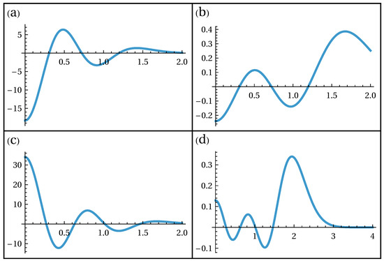
Figure 1. $f_{{\rho }_k}\left(r\right)$ as a function of r. (a) $k=3$ and $s=-0.3$. (b) $k=3$ and $s=0.3$. (c) $k=4$ and $s=-0.3$. (d) $k=4$ and $s=0.3$. These functions have azimuthal symmetry in the complex plane.

The functions $f_{{\rho }_k}\left(r\right)$ above with k zeros, as shown in Equation (33), are the ones whose integral quantization with the Cahill–Glauber weight results in the projector operator ${\rho }_k=|k⟩⟨k|$, regardless of the value of s ($-1<s<1$). As an example, we show that if we quantize them, we again obtain the projector operator, Equation (31). We depart from Equation (16):

$$A_f={\int }_{\mathbb{C}}{\displaystyle \frac{{\mathrm{d}}^2{z}^{\prime }}{\pi }}\varpi \left(z^{\prime }\right)D\left(z^{\prime }\right){\mathfrak{f}}_{\mathfrak{s}}\left[f\right](-z^{\prime }).$$

(34)

By setting ${\mathfrak{f}}_{\mathfrak{s}}\left[{\mathfrak{f}}_{\mathfrak{s}}\left[f\right]\right]\left(z\right)=f\left(z\right)\iff {\mathfrak{f}}_{\mathfrak{s}}{\mathfrak{f}}_{\mathfrak{s}}={\mathfrak{f}}_{\mathfrak{s}}^2=I$ and using Equations (16) and (24), (34) becomes

$$A_f={\int }_{\mathbb{C}}{\displaystyle \frac{{\mathrm{d}}^2{z}^{\prime }}{\pi }}D\left(z\right)f^D(-z),$$

(35)

which is a general expression for any quantum operator yielding the corresponding classical function $f_{{\rho }_k}^D$. Let us now write the operator (35) for the case of $A_{f_{{\rho }_k}}$, that is, the quantum operator obtained from the integral quantization of the classical function (33). We replace $f_{{\rho }_k}^D(-z)$ with its expression in Equation (32), and we have

$$A_{f_{{\rho }_k}}={\int }_{\mathbb{C}}{\displaystyle \frac{{\mathrm{d}}^{2}z}{\pi }}D\left(z\right)e^{{\displaystyle \frac{-{\left|z\right|}^2}{2}}}{L}_k{\left(\right|z|}^2).$$

(36)

In order to show that this operator is an integral representation of the projector operator $|k⟩⟨k|$, we analyze the general matrix elements of the Hermitian operator $A_{f_{{\rho }_k}}$, that is,

$$⟨k^{\prime }|A_{f_{{\rho }_k}}|k^{″}⟩={\int }_{\mathbb{C}}{\displaystyle \frac{{\mathrm{d}}^{2}z}{\pi }}⟨k^{\prime }\left|D\left(z\right)\right|k^{″}⟩e^{{\displaystyle \frac{-{\left|z\right|}^2}{2}}}{L}_k{\left(\right|z|}^2),$$

(37)

where [34]

$$⟨k^{\prime }\left|D\left(z\right)\right|k^{″}⟩=\sqrt{{\displaystyle \frac{k^{″}!}{k^{\prime }!}}}{e}^{{\displaystyle \frac{-{\left|z\right|}^2}{2}}}{z}^{k^{\prime }-k^{″}}{L}_{k^{\prime }}^{(k^{\prime }-k^{″})}{\left(\right|z|}^2)for{k}^{\prime }\ge k^{″}.$$

(38)

By substituting Equation (37) into Equation (38), we obtain

$$⟨k^{\prime }|A_{f_{{\rho }_k}}|k^{″}⟩=\sqrt{{\displaystyle \frac{k^{\prime \prime }!}{k^{\prime }!}}}{\int }_{\mathbb{C}}{\displaystyle \frac{{\mathrm{d}}^{2}z}{\pi }}{e}^{-{\left|z\right|}^2}{z}^{k^{\prime }-k^{″}}{L}_k{\left(\right|z|}^2)L_{k^{\prime }}^{(k^{\prime }-k^{″})}{\left(\right|z|}^2).$$

(39)

Writing z in polar coordinates, $z=r{e}^{i\theta }$, the integration on the angular variable $\theta$, which comes from the term $z^{k^{\prime }-k^{″}}$, gives

$${\int }_0^{2\pi }{\displaystyle \frac{d\theta }{2\pi }}{e}^{i(k^{\prime }-k^{″})\theta }=\left\{\begin{array}{cc}0\hfill & if{k}^{″}\ne k^{\prime }\hfill \\ 1\hfill & if{k}^{″}=k^{\prime },\hfill \end{array}\right.$$

(40)

ensuing that only diagonal terms remain. By integrating on r, Equation (39) turns out to be

$$⟨k^{\prime }|A_{f_{{\rho }_k}}|k^{\prime }⟩={\int }_0^{\infty }drr{e}^{-r^2}{L}_k\left(r^2\right)L_{k^{\prime }}\left(r^2\right)=\left\{\begin{array}{cc}0\hfill & if{k}^{\prime }\ne k\hfill \\ 1\hfill & if{k}^{\prime }=k.\hfill \end{array}\right.$$

(41)

These are exactly the matrix elements of the operator $|k⟩⟨k|$, showing that the approach presented here works as well from classical to quantum as from quantum to classical.

Lower symbol function: For the sake of completeness, we also calculate the lower function ${\check{f}}_{{\rho }_k}\left(z\right)$ for this example:

$${\check{f}}_{{\rho }_k}\left(r\right)={\displaystyle \frac{2{(-1)}^k{(1+s)}^k}{{(1-s)}^{k+1}}}{e}^{-{\displaystyle \frac{2r^2}{1-s}}}{L}_k\left({\displaystyle \frac{4r^2}{1-s^2}}\right)(-1<s<1),$$

(42)

Note that $f_{{\rho }_k}\left(z\right)$ and ${\check{f}}_{{\rho }_k}\left(z\right)$ above are the same when $s=0$, which is the Wigner function. For any other value of $-1<s<1$, $f_{{\rho }_k}\left(r\right)$ and ${\check{f}}_{{\rho }_k}\left(r\right)$ become one another when $s\to -s$.

4.1.2. Mixed State

Let us now examine the example of a mixed state. We consider two harmonic oscillators, $O_1$ and $O_2$, with corresponding classical phase space, represented by $z_1$ and $z_2$, and quantum Hilbert space, where the operators are $a_1$, $a_1^{†}$ and $a_2$, $a_2^{†}$, $[a_i,a_j^{†}]={\delta }_{ij}$, with $i,j=1,2$. The quantum states of the composed system are given by the tensor product of the states of the Hamiltonian of $O_1$ with the Hamiltonian of $O_2$ and are represented by the vectors $\left\{\right|k_1,k_2⟩\}\equiv \left\{\right|k_1⟩⨂\left|k_2\right\}$. We choose to study the following density operator associated with the mixed state of the states $|01⟩$ and $|10⟩$:

$${\rho }_{01}={\displaystyle \frac{1}{2}}\left(\right|01⟩⟨01|+|10⟩⟨10\left|\right).$$

(43)

In this case, the Cahill–Glauber weight for the two oscillators is

$$\varpi (z_1,z_2)=\varpi (r_1,r_2)=e^{{\displaystyle \frac{s_1{r}_1^2+s_2{r}_2^2}{2}}},$$

(44)

where $z_1$ and $z_2$ are the coordinates on $\mathbb{C}$ of the oscillators $O_1$ and $O_2$, respectively, and $z_1$, $z_2$ are given by Equation (1) in the phase-space coordinates $q_1,p_1$ and $q_2,p_2$ and $r_i^2={\left|z_i\right|}^2$, $-1<s_i<1$, $i=1,2$. In the following calculations, we choose the particular case of $s_1=s_2=s$. The displacement operator $D(z_1,z_2)$ for the case of two independent oscillators is written as

$$\begin{array}{cc}\hfill D(z_1,z_2)=& e^{z_1{a}_1^{†}-\overline{z_1}{a}_1}{e}^{z_2{a}_2^{†}-\overline{z_2}{a}_2}\hfill \\ \hfill =& e^{-{\displaystyle \frac{1}{2}}\left(\right|z_1{|}^2+|z_2{|}^2)}{e}^{z_1{a}_1^{†}}{e}^{-{\overline{z}}_1{a}_1}{e}^{z_2{a}_2^{†}}{e}^{-{\overline{z}}_2{a}_2}.\hfill \end{array}$$

(45)

The definition (Equation (21)) for the case of two oscillators takes the form $f_{01}^D(z_1,z_2)=tr\left[D(z_1,z_2){\rho }_{01}\right]$, and we obtain the following function for the density operator (43):

$$f_{01}^D(r_1,r_2)=e^{-{\displaystyle \frac{r_1^2+r_2^2}{2}}}\left[1-{\displaystyle \frac{1}{2}}\left(r_1^2+r_2^2\right)\right],$$

(46)

where $r_i^2={\left|z_i\right|}^2$, $i=1,2$.

From Definition (24), the expression above for $f_{01}^D(r_1,r_2)$, and the weight function (44) with $s_1=s_2=s$, we obtain the original function $f_{01}$ associated with the density operator (43):

$$f_{01}(r_1,r_2)=4e^{-{\displaystyle \frac{2(r_1^2+r_2^2)}{1+s}}}\left[{\displaystyle \frac{s^2-1+2(r_1^2+r_2^2)}{{(1+s)}^4}}\right].$$

(47)

By ’associated,’ we mean that if we apply the integral quantization method through either Equation (13) or Equation (16) to the $f_{01}(r_1,r_2)$ function above, with the weight function Equation (44), we obtain the density operator ${\rho }_{01}$ (Equation (43)). In Figure 2, we show the behavior of $f_{01}(r,r)$ for $s=0.3$.

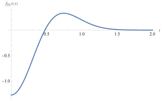
Figure 2. Function $f_{01}(r,r)$ as a function of r for $s=0.3$.

Lower symbol function:

Using the definition of the Fourier transform, Equation (15), and the expression for the $f_{01}^D$ function, Equation (46), we can also easily calculate the lower symbol, Equation (27), for this case, obtaining the expression

$${\check{f}}_{01}(r_1,r_2)=4e^{-{\displaystyle \frac{2(r_1^2+r_2^2)}{1-s}}}\left[{\displaystyle \frac{s^2-1+2(r_1^2+r_2^2)}{{(1-s)}^4}}\right].$$

(48)

Here, again, $f_{01}(r_1,r_2)$ and ${\check{f}}_{01}(r_1,r_2)$ transform into one another when we change $s\to -s$. This is due to the fact that in order to obtain $f_A$, we divide $f^D$ by $\varpi$, Equation (24), and in order to obtain $\check{f}$, we multiply $f^D$ by $\varpi$, Equation (27). So, $s\to -s$.

4.1.3. Annihilation Operator a

Up to now, we have discussed phase-independent operators. For the sake of completeness, we will now discuss the annihilation operator a, which is phase-dependent.

For this, let us consider a Hilbert space of a harmonic oscillator ${\mathcal{H}}_{HO}$ and the operators a and $a^{†}$ acting on the states $\left\{\right|k⟩\}$ of this Hilbert space. Notice that with the operators a and $a^{†}$ satisfying $[a,a^{†}]=I$ ($\hslash =1$), we can construct the operators Q and P, which are non-commutative. When, using our method, we find the corresponding function $f(q,p)$ in the classical phase space of these operators, the variables $(q,p)$ become commutative, in a simpletic manifold. This clearly shows the compatibility of the inverse formalism developed in this manuscript with the deformation of the Poisson bracket of a classical system.

First, we have to calculate the corresponding $f_a^D\left(z\right)$ function. By definition,

$$f_a^D\left(z\right)=Tr\left[D\left(z\right)a\right]=\sum _{n\ge 0}⟨n\left|D\left(z\right)a\right|n⟩=\sum _{n\ge 1}\sqrt{n}⟨n\left|D\left(z\right)\right|n-1⟩$$

(49)

and we immediately find that

$$f_a^D\left(z\right)=\sum _{n\ge 1}{e}^{{\displaystyle \frac{-{\left|z\right|}^2}{2}}}z{L}_{n-1}^1{\left(\right|z|}^2),$$

(50)

since $⟨n\left|D\left(z\right)\right|n-1⟩=\sqrt{1/n}{exp(-|z|}^2/2)z{L}_{n-1}^1{\left(\right|z|}^2)$. $L_{n-1}^1\left(x\right)$ is the generalized Laguerre polynomial $L_{n-1}^{\beta }\left(x\right)$ with $\beta =1$. Considering the Glauber–Cahill weight, Equation (30), from Equation (24), we find the function $f_a\left(z\right)$ in the complex plane that corresponds to the annihilation operator a, obtained from the symplectic Fourier transform of $f_a^D/\varpi$ as follows:

$$\begin{array}{cc}\hfill f_a\left(z\right)=& {\mathfrak{f}}_{\mathfrak{s}}\left[{\displaystyle \frac{f_a^D}{\varpi }}\right]\left(z\right)={\int }_{\mathbb{C}}{\displaystyle \frac{d^2{z}^{\prime }}{\pi }}{e}^{z\circ z^{\prime }}{\displaystyle \frac{f_a^D\left(z^{\prime }\right)}{\varpi \left(\right|z^{\prime }\left|\right)}}\hfill \\ \hfill =& \sum _{n\ge 1}{\int }_{\mathbb{C}}{\displaystyle \frac{r^{\prime }d{r}^{\prime }d{\theta }^{\prime }}{\pi }}{e}^{2\mathsf{i}r{r}^{\prime }sin(\theta -{\theta }^{\prime })}{e}^{-{\displaystyle \frac{(1+s){\left(r^{\prime }\right)}^2}{2}}}{r}^{\prime }{e}^{\mathsf{i}{\theta }^{\prime }}{L}_{n-1}^1\left({\left(r^{\prime }\right)}^2\right).\hfill \end{array}$$

(51)

The integration on ${\theta }^{\prime }$ can be done with the help of the following relation:

$${\int }_0^{2\pi }{\displaystyle \frac{d{\theta }^{\prime }}{2\pi }}{e}^{\mathsf{i}{\theta }^{\prime }+\mathsf{i}2r{r}^{\prime }sin(\theta -{\theta }^{\prime })}=e^{\mathsf{i}\theta }{J}_1\left(2r{r}^{\prime }\right)$$

(52)

where $J_n\left(x\right)$ is the Bessel function of the first kind, and Equation (51) turns into

$$\begin{array}{cc}\hfill f_a\left(z\right)=& \sum _{n\ge 1}{e}^{\mathsf{i}\theta }{\int }_0^{\infty }d{r}^{\prime }{e}^{-{\displaystyle \frac{(1+s){\left(r^{\prime }\right)}^2}{2}}}{\left(r^{\prime }\right)}^2{L}_{n-1}^1\left({\left(r^{\prime }\right)}^2\right)J_1\left(2r{r}^{\prime }\right)\hfill \end{array}$$

(53)

$$\begin{array}{cc}\hfill & =r{e}^{\mathsf{i}\theta }\left({\displaystyle \frac{4}{s^2-1}}\right)e^{-{\displaystyle \frac{2r^2}{1+s}}}\sum _{n\ge 1}{\left({\displaystyle \frac{s-1}{s+1}}\right)}^n{L}_{n-1}^{\left(1\right)}\left({\displaystyle \frac{4r^2}{1-s^2}}\right).\hfill \end{array}$$

(54)

Using the result,

$$\sum _{n\ge 1}{\left({\displaystyle \frac{s-1}{s+1}}\right)}^n{L}_{n-1}^1\left({\displaystyle \frac{4r^2}{1-s^2}}\right)=\left({\displaystyle \frac{s^2-1}{4}}\right)e^{{\displaystyle \frac{2r^2}{1+s}}},$$

(55)

we finally get the function in the complex plane that corresponds to the annihilation operator a,

$$f_a\left(z\right)=r{e}^{\mathsf{i}\theta }=z,$$

(56)

showing that the $f_a^D$ function correctly gives the function in the complex plane, $f_a\left(z\right)=z$, which, when quantized, results in the annihilation operator a [2].

Clearly, the creation operator is associated with the function $f_{a^{†}}\left(z\right)=\overline{z}$.

4.1.4. Entangled State

Another important feature of the quantization procedure and its reverse counterpart is the possibility of visualizing the effects of quantum entanglement in the classical phase space.

In order to visualize these effects, let us consider two harmonic oscillators, with Hamiltonians ${\mathcal{H}}_1$ and ${\mathcal{H}}_2$, with quantum states $\left\{\right|k_1⟩\}$ and $\left\{\right|k_2⟩\}$, where $k_i$, $i=1,2$, represents the $k_i$ level of the system i, respectively. The states of the tensor product of $\mathcal{H}={\mathcal{H}}_1⨂{\mathcal{H}}_2$ are represented by $\left\{\right|k_1,k_2⟩\}\equiv \left\{\right|k_1⟩⨂\left|k_2\right\}$. As an example, consider the density operator of a pure entangled state

$${\rho }_{{\Psi }^{+}}={\displaystyle \frac{1}{2}}\left(|01⟩⟨01|+|01⟩⟨10|+|10⟩⟨01|+|10⟩⟨10|\right),$$

(57)

which was obtained through ${\rho }_{{\psi }^{+}}=|{\Psi }^{+}⟩⟨{\Psi }^{+}|$, where $|{\Psi }^{+}⟩={\displaystyle \frac{1}{\sqrt{2}}}\left(|01⟩+|10⟩\right)$ is one of the usual Bell’s states. As with the case of a mixed state (Section 4.1.2), the function $f_{{\Psi }^{+}}^D(z_1,z_2)=tr\left[D(z_1,z_2){\rho }_{{\Psi }^{+}}\right]$ can be obtained for the density operator Equation (57),

$$f_{{\psi }^{+}}^D(z_1,z_2)=e^{{\displaystyle \frac{-|z_1{|}^2-{\left|z_2\right|}^2}{2}}}\left[1-{\displaystyle \frac{1}{2}}\left(|z_1{|}^2+{\left|z_2\right|}^2+{\overline{z}}_1{z}_2+z_1{\overline{z}}_2\right)\right],$$

(58)

which turns into

$$f_{{\psi }^{+}}(z_1,z_2)={\displaystyle \frac{4e^{\frac{-2(r_1^2+r_2^2)}{(s+1)}}}{{(s+1)}^4}}\left[s^2-1+2\left(r_1^2+r_2^2+2r_1{r}_{2}cos({\theta }_1-{\theta }_2)\right)\right],$$

(59)

where $z_j=r_j{e}^{i{\theta }_j}$, and $s_1=s_2=s$. When one compares Equations (59) and (47), it is obvious that the only difference is the extra last term on the right-hand side of Equation (59), which couples the phases of $z_1$ and $z_2$. In order to visualize the behavior of the phase-space function f, we set $r_1=r_2=r$ and plot the result in Figure 3, where the axes are $rcos\Delta \theta$ and $rsin\Delta \theta$, and $\Delta \theta ={\theta }_1-{\theta }_2$. This observation leads us to state that quantum correlations appear in the classical phase space as the absence of radial symmetry. In other words, the quantum nature of a system is reflected in the function f that is not invariant during rotations.

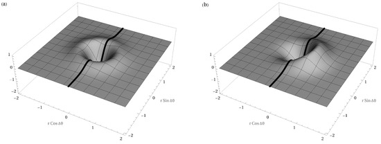
Figure 3. Plot of the classical phase space function f for (a) the mixed state (Equation (47)) and for (b) the entangled pure state (Equation (59)). We set $s=0.3$, $r_1=r_2=r$, and $\Delta \theta ={\theta }_1-{\theta }_2$. The mixed-state case does not depend on $\Delta \theta$; therefore, it is invariant under the effect of rotations. The black curve in (b) corresponds to $\Delta \theta =\pi /2$ and $3\pi /2$; it is exactly the same curve as in (a).

For the sake of completeness, we can analyze the other Bell states. For example, ${\rho }_{{\psi }^{-}}=|{\Psi }^{-}⟩⟨{\Psi }^{-}|$ where $|{\Psi }^{-}⟩={\displaystyle \frac{1}{\sqrt{2}}}\left(|01⟩-|10⟩\right)$, which gives the auxiliary function

$$f_{{\psi }^{-}}^D(z_1,z_2)=e^{{\displaystyle \frac{-|z_1{|}^2-{\left|z_2\right|}^2}{2}}}\left[1-{\displaystyle \frac{1}{2}}\left(|z_1{|}^2+{\left|z_2\right|}^2-{\overline{z}}_1{z}_2-z_1{\overline{z}}_2\right)\right],$$

(60)

and the classical phase space function

$$f_{{\psi }^{-}}(z_1,z_2)={\displaystyle \frac{4e^{\frac{-2(r_1^2+r_2^2)}{(s+1)}}}{{(s+1)}^4}}\left[s^2-1+2\left(r_1^2+r_2^2-2r_1{r}_{2}cos({\theta }_1-{\theta }_2)\right)\right].$$

(61)

The other entangled density matrices ${\rho }_{{\varphi }^{\pm }}=|{\Phi }^{\pm }⟩⟨{\Phi }^{\pm }|$ are related to the two Bell states $|{\Phi }^{\pm }⟩={\displaystyle \frac{1}{\sqrt{2}}}\left(|00⟩\pm |11⟩\right)$, which have an auxiliary function of the form

$$\begin{array}{c}\hfill f_{{\varphi }^{\pm }}^D(z_1,z_2)={\displaystyle \frac{1}{2}}{e}^{{\displaystyle \frac{-|z_1{|}^2-{\left|z_2\right|}^2}{2}}}\left[1+\left(1-|z_1{|}^2\right)\left(1-|z_2{|}^2\right)\pm z_1{z}_2\pm {\overline{z}}_1{\overline{z}}_2\right],\end{array}$$

(62)

and its respective classical phase space function

$$\begin{array}{cc}\hfill f_{{\varphi }^{\pm }}(z_1,z_2)={\displaystyle \frac{4e^{\frac{-|z_1{|}^2-{\left|z_2\right|}^2}{2}}}{{(1+s)}^6}}& \left[1-2r_1^2-2r_2^2+8r_1^2{r}_2^2+2s+2\left(r_1^2+r_2^2+1\right)s^2\right.\hfill \\ & \left.+2s^3+s^4\pm 4r_1{r}_2{(s+1)}^{2}cos\left({\theta }_1+{\theta }_2\right)\right].\hfill \end{array}$$

(63)

4.1.5. Discussion

In this section, we clarify how the angular dependence of the classical phase space function is generated by the density matrix. To simplify the notation, the states $|00⟩,|01⟩,|10⟩,|11⟩$ are encoded as $|0⟩,|1⟩,|2⟩,|3⟩$, respectively. Then, we can write the product

$$D_{mn}\left(z_1\right)D_{m^{\prime }{n}^{\prime }}\left(z_2\right)={\mathfrak{D}}_{ij}(z_1,z_2),$$

(64)

where $m,n,m^{\prime },n^{\prime }=0, 1$; $i,j=0,1,2,3$; and the relation between $m{m}^{\prime }\left(n{n}^{\prime }\right)$ and $i\left(j\right)$ is the usual conversion of a number from base 2 to base 10. Then, any density matrix elements of a two-qbit system ${\rho }_{m{m}^{\prime }n{n}^{\prime }}=⟨m{m}^{\prime }\left|\rho \right|n{n}^{\prime }⟩$ can be written as ${\rho }_{ij}=⟨i\left|\rho \right|j⟩$. So, the auxiliary function

$$f_{\rho }^D(z_1,z_2)=Tr\left[D(z_1,z_2)\rho \right]=\sum _{i,j=0}^3{\mathfrak{D}}_{ij}(z_1,z_2){\rho }_{ji},$$

(65)

where ${\mathfrak{D}}_{ij}=⟨i|D(z_1,z_2)|j⟩$ and $D(z_1,z_2)$ are given by Equation (45), can be employed to find the classical phase-space function $f_{\rho }$ via the transformation defined in Equation (24) (applied twice for each variable $z_1$ and $z_2$):

$$f_{\rho }(z_1,z_2)=\sum _{i,j=0}^3{\tilde{\mathfrak{D}}}_{ij}(z_1,z_2){\rho }_{ji},$$

(66)

where

$$\begin{array}{ccc}\hfill {\tilde{\mathfrak{D}}}_{ij}(z_1,z_2)& =& {\mathfrak{f}}_{\mathfrak{s}}\left[{\mathfrak{f}}_{\mathfrak{s}}\left[{\displaystyle \frac{{\mathfrak{D}}_{ij}({\xi }_1,{\xi }_2)}{\omega (-{\xi }_1)\omega (-{\xi }_2)}}\right]\left(z_1\right)\right]\left(z_2\right)\hfill \end{array}$$

(67)

$$\begin{array}{ccc}& =& {\mathfrak{f}}_{\mathfrak{s}}\left[{\displaystyle \frac{D_{mn}\left({\xi }_1\right)}{\omega (-{\xi }_1)}}\right]\left(z_1\right){\mathfrak{f}}_{\mathfrak{s}}\left[{\displaystyle \frac{D_{m^{\prime }{n}^{\prime }}\left({\xi }_2\right)}{\omega (-{\xi }_2)}}\right]\left(z_2\right)\hfill \end{array}$$

(68)

$$\begin{array}{ccc}& =& {\tilde{D}}_{mn}\left(z_1\right){\tilde{D}}_{m^{\prime }{n}^{\prime }}\left(z_2\right),\hfill \end{array}$$

(69)

where ${\tilde{D}}_{mn}\left(z_1\right)={\mathfrak{f}}_{\mathfrak{s}}\left[{\displaystyle \frac{D_{mn}\left({\xi }_1\right)}{\omega (-{\xi }_1)}}\right]\left(z_1\right)$. The sum of Equation (66) can be separated in two terms, one related to the population of the density operator ${\rho }_{ii}$ and the other with the coherence terms ${\rho }_{ji}$:

$$f_{\rho }(z_1,z_2)=\sum _{i=0}^3{\tilde{\mathfrak{D}}}_{ii}(z_1,z_2){\rho }_{ii}+\sum _{i\ne j}{\tilde{\mathfrak{D}}}_{ij}(z_1,z_2){\rho }_{ji}.$$

(70)

Consider the terms of the first sum ${\tilde{\mathfrak{D}}}_{ii}(z_1,z_2)$:

$$\begin{array}{cc}\hfill {\tilde{\mathfrak{D}}}_{ii}(z_1,z_2)=& {\tilde{D}}_{mm}\left(z_1\right){\tilde{D}}_{m^{\prime }{m}^{\prime }}\left(z_2\right)\hfill \end{array}$$

(71)

$$\begin{array}{cc}\hfill =& {\mathfrak{f}}_{\mathfrak{s}}\left[{\displaystyle \frac{D_{mm}\left({\xi }_1\right)}{\omega (-{\xi }_1)}}\right]\left(z_1\right){\mathfrak{f}}_{\mathfrak{s}}\left[{\displaystyle \frac{D_{m^{\prime }{m}^{\prime }}\left({\xi }_2\right)}{\omega (-{\xi }_2)}}\right]\left(z_2\right),\hfill \end{array}$$

(72)

note that ${\tilde{\mathfrak{D}}}_{ii}(z_1,z_2)$ depends solely on the functions $D_{mm}\left({\xi }_1\right)$ and $D_{m^{\prime }{m}^{\prime }}\left({\xi }_2\right)$. These functions (see Equation (38)), along with their symplectic Fourier transforms, exhibit no angular dependence. Consequently, ${\tilde{\mathfrak{D}}}_{ii}(z_1,z_2)$ is independent of the angle. On the other hand, the terms ${\tilde{\mathfrak{D}}}_{ij}(z_1,z_2)$ in the second sum of Equation (70) with $i\ne j$ are related to the functions $D_{mn}\left({\xi }_1\right)$ and $D_{m^{\prime }{n}^{\prime }}\left({\xi }_2\right)$, with $m\ne n$ or $m^{\prime }\ne n^{\prime }$. Then, at least one of these functions (and its symplectic Fourier transform) has angle dependence. Therefore, the nonzero values of the coherent terms of the density operator ${\rho }_{ji}$ are responsible for the angle dependency of the function $f_{\rho }(z_1,z_2)$.

We observe that ${\tilde{\mathfrak{D}}}_{ii}(z_1,z_2)$ is determined exclusively by $D_{mm}\left({\xi }_1\right)$ and $D_{m^{\prime }{m}^{\prime }}\left({\xi }_2\right)$ (see Equation (38)). Since these quantities and their symplectic Fourier transforms lack angular dependence, ${\tilde{\mathfrak{D}}}_{ii}(z_1,z_2)$ remains angle-independent. In contrast, the cross terms ${\tilde{\mathfrak{D}}}_{ij}(z_1,z_2)$ ($i\ne j$) in the second sum of Equation (70) involves $D_{mn}\left({\xi }_1\right)$ and $D_{m^{\prime }{n}^{\prime }}\left({\xi }_2\right)$, where $m\ne n$ or $m^{\prime }\ne n^{\prime }$. Here, at least one of these functions(or its symplectic Fourier transform) exhibits angular variation. Thus, the non-vanishing coherent terms ${\rho }_{ji}$ in the density operator introduce angle dependence into $f_{\rho }(z_1,z_2)$, which is the relation between the entanglement and the phases in the classical phase-space function.

4.2. An Alternative Weight

In this section, we introduce the following alternative weight,

$$w_2\left(z\right)={\displaystyle \frac{e^{{\frac{\sigma \left|z\right|}{2}}^2}}{1+{\left|z\right|}^2}},0\le \left|z\right|<\infty ,$$

(73)

in order to analyze the influence of different possible weights on the behavior of the classical functions $f\left(z\right)$. As an example, we show the classical function obtained with this alternative weight only for the case of the projector operator $|k⟩⟨k|$ for, respectively, $k=2$,

$$\begin{array}{cc}\hfill f_{{\rho }_2}^{w_2}\left(z\right)=& {\displaystyle \frac{e^{-\frac{2r^2}{\sigma +1}}}{{(\sigma +1)}^7}}\left[-32r^6+24r^4(1+\sigma )(5-\sigma )+4r^2{(1+\sigma )}^2\left({\sigma }^2+14\sigma -23\right)\right.\hfill \\ \hfill & \left.+{(1+\sigma )}^3\left({\sigma }^3+{\sigma }^2-13\sigma +11\right)\right],\hfill \end{array}$$

(74)

and $k=3$,

$$\begin{array}{cc}\hfill f_{{\rho }_3}^{w_2}\left(z\right)=& {\displaystyle \frac{e^{-\frac{2r^2}{\sigma +1}}}{3{(\sigma +1)}^9}}\left[-128r^8+256r^6(1+\sigma )(3-\sigma )-72r^4{(1+\sigma )}^2({\sigma }^2-14\sigma +17)\right.\hfill \\ \hfill & \left.+24r^2{(1+\sigma )}^3({\sigma }^3+9{\sigma }^2-33\sigma +23)+{(1+\sigma )}^4(3{\sigma }^4-54{\sigma }^2+96\sigma -45)\right].\hfill \end{array}$$

(75)

The plot for the case where $k=3$ for Cahill–Glauber and $w_2$ weights can be seen in Figure 4 for $s=\sigma =-0.3$. Notice that using different weights changes only the amplitude and the values of the functions when crossing the abscissa axis, and therefore they are not important. What remains unchanged for different weights, and is thus the important feature, is the number of oscillations (crosses of the abscissa axis). In the present case, this number is three.

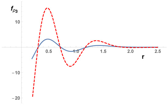
Figure 4. Classical functions $f_{{\rho }_3}\left(r\right)$ corresponding to the quantum projector operator $|3⟩⟨3|$ as functions of r. The blue (continuous) line was obtained with the Cahill–Glauber weight, and the red (dashed) one was obtained with the $w_2$ weight.

It would be valuable to extend the analysis of this alternative weight to the other operators studied in this work—namely, the mixed state, annihilation operator, and entangled state—in order to identify which properties of the corresponding classical functions are universal (i.e., independent of the quantization scheme) and which are contingent on the choice of weight. Such an investigation would help distinguish between intrinsic features of the quantum–classical correspondence and artifacts of the particular quantization method employed.

5. Conclusions

A wide variety of quantization methods have been proposed over the years, with no single criterion to definitively select the most suitable one. Among these, integral quantization—first introduced by Weyl in 1927—stands out as a powerful approach capable of quantizing classical functions in situations where the canonical method fails.

In modern formulations of integral quantization, the introduction of a weight function plays a crucial role. This function unifies different quantization schemes—such as Wigner–Weyl and coherent state quantization—by expressing them as special cases corresponding to particular parameter choices. Moreover, the formalism naturally defines a lower symbol function $\check{f}$, which maps an operator back to the classical phase space while preserving the quantum expectation values of the original observable. However, in general, this lower symbol does not coincide with the initial classical function from which the operator was derived.

In this work, we have addressed the inverse problem: given an operator A in a Hilbert space—expressed as a function of Q and P—how can one determine a classical phase-space function $f_A\left(z\right)$ (or equivalently $f_A(q,p)$) whose quantization reproduces exactly the same operator A? Answering this question allows us to associate a classical counterpart with an arbitrary quantum operator, provided it is built from Q and P. This is particularly useful for operators—such as projectors or certain density matrices—whose classical origin is not immediately obvious. Notably, this approach does not apply to purely quantum degrees of freedom, such as spin.

To this end, we introduced a method based on a newly defined auxiliary function $f_A^D\left(z\right)=\mathrm{Tr}\left[D\left(z\right)A\right]$, which is straightforwardly related to the desired classical function $f_A\left(z\right)$ via a symplectic Fourier transform incorporating the chosen weight function (which is assumed to have no zeros). Quantizing $f_A\left(z\right)$ then returns the original operator A, completing the round-trip from quantum to classical and back.

We applied this method to several important operators using the Cahill–Glauber weight: a number-state projector, a mixed-state density operator, an entangled-state density operator, and the annihilation operator. In each case, we derived the corresponding classical function and verified that its quantization recovers the original operator. To assess the influence of the weight function, we also examined an alternative weight for the projector case. Our results show that the number of oscillations (or nodes) of the classical function $f_{{\rho }_k}$ is independent of the weight, whereas the amplitude and the precise locations of the zeros are weight-dependent. Furthermore, by comparing the entangled- and mixed-state examples, we demonstrated that angular dependence in the classical phase-space function $f_{{\rho }_e}$ serves as a signature of quantum entanglement in the corresponding density operator ${\rho }_e$.

Thus, we have worked with two distinct classical representations of a quantum operator: the established lower symbol ${\check{f}}_A$, which preserves expectation values, and the new function $f_A^D$ (and its derived $f_A$), which allows recovery of the original operator under quantization. The latter is especially valuable when the operator’s classical origin is unknown or unclear.

We hope this investigation contributes to clarifying the ever-subtle relationship between classical and quantum descriptions of physical systems [29,30]. Future work may extend this approach to open quantum systems and more general phase-space geometries.

References

- Ali, S.T.; Englis, M. Quantization Methods: A Guide for Physicists and Analysts. Rev. Math. Phys. 2004, 17, 391490. [Google Scholar] [CrossRef]
- Bergeron, H.; Gazeau, J.P.; Youssef, A. To what extent are canonical and coherent state quantizations physically equivalent? Phys. Lett. 2018, 377, 598. [Google Scholar] [CrossRef]
- Gazeau, J.P. Coherent States in Quantum Physics; Wiley-VCH: Berlin, Germany, 2009. [Google Scholar]
- Berezin, F.A. General Concept of Quantization. Commun. Math. Phys. 1975, 40, 153. [Google Scholar] [CrossRef]
- Gazeau, J.P.; Klauder, J.R. Coherent states for systems with discrete and continuous spectrum. Phys. A Math. Gen. 1999, 32, 123. [Google Scholar] [CrossRef]
- Klauder, J.R. Beyond Conventional Quantization; Cambridge University Press: Cambridge, UK, 2000. [Google Scholar]
- Gazeau, J.P. From Classical to Quantum Models: The Regularising Rôle of Integrals, Symmetry and Probabilities. Found. Phys. 2018, 48, 1648–1667. [Google Scholar] [CrossRef]
- Groenewold, H. On the Principles of Elementary Quantum Mechanics. Physica 1946, 12, 405–460. [Google Scholar] [CrossRef]
- Hove, L.V. Sur le probleme des relations entre les transformations unitaires de la mécanique quantique et les transformations canoniques de la mécanique classique. Bull. L’académie R. Belg. 1951, 5, 610–620. [Google Scholar]
- Weyl, H. Quantenmechanik und Gruppentheorie. Z. Phys. 1927, 46, 1. [Google Scholar] [CrossRef]
- Wigner, E. On the Quantum Correction For Thermodynamic Equilibrium. Phys. Rev. 1932, 40, 749. [Google Scholar] [CrossRef]
- Souriau, J.-M. Structure de Sisteme Dynamique; Dunod: Paris, France, 1969. [Google Scholar]
- Kostant, B. Quantization and Unitary Representations; Lecture Notes in Mathematics; Springer: Berlin, Germany, 1970. [Google Scholar]
- Kirillov, A.A. Elements of the Theory of Representations, 2nd ed; Nauka: Moscow, Russia, 1978. (In Russian) English translation of the 1st edition: Grundlehren der Mathematischen Wissenschaften, Band 220; Springer: Berlin, Germany; New York, NY, USA, 1976. [Google Scholar]
- Bates, S.; Weinstein, A. Lectures on the Geometry of Quantization; Berkeley Mathematics Lecture Notes; American Mathematical Society: Providence, RI, USA, 1997; Volume 8. [Google Scholar]
- Kostant, B. Collected Papers: 1955–1966; Springer: New York, NY, USA, 2009. [Google Scholar]
- Bayen, F.; Flato, M.; Fronsdal, C.; Lichnerowicz, A.; Sternheimer, D. Deformation theory and quantization. Ann. Phys. 1978, 111, 61–151. [Google Scholar] [CrossRef]
- Fedosov, B.V. A simple geometric construction of deformation quantization. J. Diff. Geo. 1994, 40, 213–238. [Google Scholar]
- Gutt, S. Deformation Quantization and Group Actions. In Quantization, Geometry and Noncommutative Structures in Mathematics and Physics; Mathematical Physics Studies; Cardona, A., Morales, P., Ocampo, H., Paycha, S., Reyes Lega, A., Eds.; Springer: Cham, Switzerland, 2017. [Google Scholar]
- Waldmann, S. Recent Developments in Deformation Quantization. In Quantum Mathematical Physics; Finster, F., Kleiner, J., Röken, C., Tolksdorf, J., Eds.; Birkhäuser: Cham, Switzerland, 2016. [Google Scholar]
- Bergeron, H.; Gazeau, J.P. Integral quantizations with two basic examples. Ann. Phys. 2014, 344, 43–68. [Google Scholar] [CrossRef]
- Baldiotti, M.C.; Fresneda, R.; Gazeau, J.-P. Dirac distribution and Dirac constraint quantizations. Phys. Scr. 2015, 90, 074039. [Google Scholar] [CrossRef]
- Gazeau, J.P.; Baldiotti, M.C.; Fresneda, R. Three examples of covariant integral quantization. In Proceedings of the 3d International Satellite Conference on Mathematical Methods in Physics—ICMP 2013, Londrina, PR, Brazil, 21–26 October 2013. [Google Scholar]
- Weinbub, J.; Ferry, D.K. Recent advances in Wigner function approaches. Appl. Phys. Rev. 2018, 5, 041104. [Google Scholar] [CrossRef]
- Koczor, B.; vom Ende, F.; de Gosson, M.; Glaser, S.J.; Zeier, R. Phase Spaces, Parity Operators, and the Born-Jordan Distribution. In Annales Henri Poincaré; Springer: Cham, Switzerland, 2023; pp. 4169–4236. [Google Scholar]
- Nelson, E. On the derivation of the Schrödinger equation from Newtonian mechanics. Phys. Rev. 1966, 150, 1079–1080. [Google Scholar]
- de la Pena, L.; Cetto, A.M. The Quantum Dice; Springer: Cham, Switzerland, 1996. [Google Scholar]
- Bayer, M.; Paul, W. On the Stochastic Mechanics Foundation of Quantum Mechanics. Universe 2021, 7, 166. [Google Scholar] [CrossRef]
- Brody, D.C.; Graefe, E.-M.; Melanathuru, R. Phase-Space Measurements, Decoherence, and Classicality. Phys. Rev. Lett. 2025, 134, 120201. [Google Scholar] [CrossRef] [PubMed]
- Bibak, F.; Cepollaro, C.; Sánchez, N.M.; Dakić, B.; Brukner, Č. The classical limit of quantum mechanics through coarse-grained measurements. arXiv 2025, arXiv:2503.15642. [Google Scholar] [CrossRef]
- Todorov, I. Quantization is a Mystery. arXiv 2012, arXiv:1206.3116. [Google Scholar] [CrossRef]
- Ali, S.T.; Antoine, J.P.; Gazeau, J.P. Coherent States, Wavelets, and Their Generalizations, 2nd ed.; Springer: New York. NY, USA, 2014. [Google Scholar]
- Carosso, A. Quantization: History and Problems. Stud. Hist. Philos. Sci. 2022, 96, 35–50. [Google Scholar] [CrossRef]
- Bergeron, H.; Curado, E.M.F.; Gazeau, J.P.; Rodrigues, L.M.C.S. Weyl-Heisenberg Integral Quantization(s): A Compendium. arXiv 2017, arXiv:1703.08443. [Google Scholar]
- Cahill, K.E.; Glauber, R.J. Density Operators in Quasiprobability Distributions. Phys. Rev. 1969, 177, 1882. [Google Scholar] [CrossRef]
Disclaimer/Publisher’s Note: The statements, opinions and data contained in all publications are solely those of the individual author(s) and contributor(s) and not of MDPI and/or the editor(s). MDPI and/or the editor(s) disclaim responsibility for any injury to people or property resulting from any ideas, methods, instructions or products referred to in the content. |
© 2026 by the authors. Licensee MDPI, Basel, Switzerland. This article is an open access article distributed under the terms and conditions of the Creative Commons Attribution (CC BY) license.