Time-Dependent Probability Distribution of Two-Dimensional Moran Walk

Abstract

In this paper, we introduce and analyze a novel two-dimensional Moran random walk model, where each component evolves by either increasing by one unit or resetting to zero at each time step, with transition probabilities dependent on time. The primary contribution of this work is the derivation of an explicit closed-form expression for the probability distribution of the final maximum altitude, $U_n=max(U_n^{\left(1\right)},U_n^{\left(2\right)})$. Additionally, we provide a detailed analysis of the height statistics and cumulative distribution associated with the model. Using probabilistic techniques, we establish the exact distribution of the final altitude and its moments. Furthermore, we conduct numerical simulations to illustrate the behavior of the model for various parameter values. These results offer new insights into the statistical properties of two-dimensional Moran processes and have potential applications in population genetics, nuclear physics, and related fields.

1. Introduction

Moran processes model population evolution (or mutation transmission) in a fixed-size population, where any individual that dies is immediately replaced by a new one. Various adaptations of the original process, introduced by Moran [1,2], have been explored in the literature, including more recent extensions such as those incorporating spatially structured populations [3]. Motivated by the literature, we define in this paper a new model of the Moran random walk in two dimensions. The two-dimensional Moran model is a mathematical framework used to study the evolution of allele frequencies in a population of two distinct types (alleles). The “symmetric” aspect typically implies that the population size remains constant, and each individual has an equal probability of reproducing. The Moran model is often used in population genetics. At each time step n, each individual can jump to the next level $+1$ with a probability that depends on n and reset to 0 with a complementary probability.

In the literature, the statistical properties, including the limiting distribution, the mean, the variance and the cumulative function, of discrete random walks are studied in many scientific papers in one or more dimensions by different methods. We can mention the kernel method and singularity analysis (see [4,5]) via some links with continued fractions [6], or via more probabilistic approaches (see [7], which also illustrates links with random trees).

For example in dimension one, we can mention the important papers in our analysis. Abdelkader [8] analyzed the height of a one-dimensional random walk and proved that the random walk converges to a shifted geometric distribution with parameter $1-p$ asymptotically. Banderier and Flajolet [4] showed that the limiting distribution of the final altitude of a random meander of length n converges to a Rayleigh distribution (drift $\delta =0$) and a normal distribution ($\delta >0$). In addition, in [9], Banderier and Nicodème studied the height of discrete bridges/meanders/excursions for discrete bounded walks. Similar extremal parameters were also studied for trees in [7,10].

For higher dimensions, still linked to our model, we can mention the two-dimensional Moran model, which was investigated by Aguech and Abdelkader in [11], where they showed that each walk converges to a shifted-geometric distribution and found their explicit expressions for the mean and the variance. In addition, they determined the exact distribution of the number of resets $N_n^X$ and the explicit expressions of the mean and variance for the final altitude walk. Althagafi and Abdelkader [12] also studied the two-dimensional Moran model and proved that the limiting distribution of the age of each component converges to a shifted geometric distribution. Furthermore, they determined the closed expressions of the mean and the variance for the final altitude (maximum age between two walks) via the probability generating function. Other articles related to the Moran process (in biology and population genetics) involve similar higher-dimensional walk models; see [13,14].

The novelty of this work compared to the existing literature is that the transition probability depends on n. To the best of our knowledge, despite its significance, this model has never been studied in the literature.

The structure of this paper is organized as follows. In Section 2, we mathematically present the two-dimensional Moran model, define the final altitude and the height statistics, denoted by $U_n$ and $H_n$, and discuss some applications. In Section 3, we state our main results concerning the probability distribution of the final altitude and the cumulative function of the height statistics associated with our model. In Section 4, we use the program R to compute the probability density function of the final altitude at time $n=25$ with three different values of the probability $q_1$: 0.1, 0.5, and 0.75. Additionally, we simulate the distribution of the final altitude at three different times, 10, 500, and 100, using $q_1$ values of 0.1, 0.5, and 0.75. In Section 5, we derive a closed-form expression for the distribution of the two components of our model. In Section 6, we present the joint probability distribution of the two components at two positive times, r and s. In Section 7, we show our main results. In Section 8, we present conclusions regarding our results and discuss future perspectives.

2. Presentation of the Model and Its Applications

In this section, we begin by introducing our two-dimensional Moran model, which is generated by a sequence of probabilities. We then present some basic definitions related to discrete random walks in one dimension, including the final statistics and height statistics. Additionally, we define the mean and variance of a discrete process.

The Moran model with two components $U_n^{\left(1\right)}$ and $U_n^{\left(2\right)}$ starts from 0 (i.e., $U_0^{\left(1\right)}=0,U_0^{\left(2\right)}=0$) at time 0 and is defined mathematically by

$$\begin{array}{cc}\hfill (U_{n+1}^{\left(1\right)},U_{n+1}^{\left(2\right)})& =\left\{\begin{array}{cc}(U_n^{\left(1\right)}+1,U_n^{\left(2\right)}+1),\hfill & \mathrm{with}\mathrm{probability}{q}_{n+1}^2,\hfill \\ (0,U_n^{\left(2\right)}+1),\hfill & \mathrm{with}\mathrm{probability}{q}_{n+1}(1-q_{n+1}),\hfill \\ (U_n^{\left(1\right)}+1,0),\hfill & \mathrm{with}\mathrm{probability}{q}_{n+1}(1-q_{n+1}),\hfill \\ (0,0),\hfill & \mathrm{with}\mathrm{probability}{(1-q_{n+1})}^2,\hfill \end{array}\right.\hfill \end{array}$$

(1)

where $q_n$ is a probability sequence defined by the following: for all $n\ge 0$

$$\left\{\begin{array}{c}{q}_0=1,q_1=q\in (0,1),\hfill \\ \\ q_n=q_{n-1}+q_{n-1}({\displaystyle \frac{9}{16}}-q_{n-1}).\hfill \end{array}\right.$$

(2)

Remark 1. 

We remark We can write $q_n=f\left(q_{n-1}\right)$, where f is defined from $[0,1]$ to $[0,1]$ by $f\left(x\right)=x+x({\displaystyle \frac{9}{16}}-x)$. It is clear that f is an increasing function from $[0,1]$ to $[0,1]$ converges to $x=9/16$, which is a fixed point of f. If we assume $q_1<3/4$, the law of $U_n^{\left(i\right)}$ will almost converge to the law of a Moran process with $q=3/4$.

We define the final altitude $U_n$, the height $H_n^{\left(i\right)}$ of the component $i=1,2$ and the height of all the walk $H_n$ by

$$\begin{array}{cc}\hfill U_n& =max(U_n^{\left(1\right)},U_n^{\left(2\right)}),\hfill \\ \hfill H_n^{\left(i\right)}& =max(U_0^{\left(i\right)},U_1^{\left(i\right)},U_2^{\left(i\right)},\dots ,U_n^{\left(i\right)}),i=1,2,\hfill \\ \hfill H_n& =max(U_0,U_1,U_2,\dots ,U_n).\hfill \end{array}$$

$U_n$, $H_n^{\left(i\right)}$, and $H_n$ are considered as discrete random walks with one dimension in the state space $\{0,\dots ,n\}$, and started from the initial state $U_0=0$, $H_0^{\left(i\right)}=0$, and $H_0=0$, respectively. But the $(U_n^{\left(1\right)},U_n^{\left(2\right)})$ are considered a stochastic process with two dimensions in the state space $S^2={\{0,\dots ,n\}}^2$, and started from the initial state $\left(0,0\right)$.

In this work, we study the probability distribution of the final altitude, denoted by $U_n$, representing the maximum age between the two components $U_n^{\left(1\right)}$ and $U_n^{\left(2\right)}$, based on the joint probability distribution of $U_n^{\left(1\right)}$ and $U_n^{\left(2\right)}$. Additionally, in this paper, we analyze the height statistics, denoted by $H_n^{\left(1\right)}$ of the first component $U_n^{\left(1\right)}$.

Our contribution is the derivation of a closed-form expression for the probability distribution of the final altitude $U_n$, given by the following: for all $k\ge 0$

$$\mathbb{P}\left(U_n=k\right)=\left\{\begin{array}{cc}{(1-q_n)}^2,\hfill & \mathrm{if}k=0,\hfill \\ {\displaystyle 2(1-q_n)(1-q_{n-k})\prod _{j=n+1-k}^n{q}_j+{(1-q_{n-k})}^2\prod _{j=n-k+1}^n{q}_j^2}\hfill \\ {\displaystyle +2\sum _{l=1}^{k-1}\left((1-q_{n-l})(1-q_{n-k})\prod _{j=0}^{l-1}{q}_{n-j}^2\prod _{j=n-k+1}^{n-l}{q}_j\right),}\hfill & \mathrm{if}1\le k<n,\hfill \\ {\displaystyle 2(1-q_n)\prod _{j=1}^n{q}_j+2\sum _{l=1}^{n-1}\left((1-q_{n-l})\prod _{j=0}^{l-1}{q}_{n-j}^2\prod _{j=1}^{n-l}{q}_j\right)+\prod _{j=1}^n{q}_j^2,}\hfill & \mathrm{if}k=n.\hfill \end{array}\right.$$

Additionally, we use the R programming language to simulate the probability distribution described earlier for specific values of n, 10, 50, and 100, and for different values of $q_1$ (0, 1, 0.5, and 0.75) of the probability $q_1$, where $q_1$ represents the first term of the sequence $q_n$ which generates our two-dimensional Moran model. Furthermore, we calculate the cumulative distribution function of the height statistics $H_n^{\left(1\right)}$ of the first component $U_n^{\left(1\right)}$, given by the following: for all $h\ge 1$

$$\mathbb{P}\left(H_n^{\left(1\right)}\le h\right)=\left(\begin{array}{cc}1,& 0\end{array}\right)·N_n\left(h\right)·\left(\begin{array}{c}{f}_1\left(h\right)\\ f_0\left(h\right)\end{array}\right),$$

where $N_n\left(h\right)=\left[{\prod }_{l=2}^n{M}_l\left(h\right)\right]$, and $M_l\left(h\right)=\left(\begin{array}{cc}1& -q_{l+1}{q}_l\\ 1& 0\end{array}\right).$

The Moran random walk is a stochastic process that models the evolution of a population across discrete generations, where individuals interact and reproduce. It is a Markov chain used in population genetics to study the changes in allele frequencies in finite populations. Some applications of the Moran random walk include the following. Population Genetics:

(1)

Allele Frequency Dynamics: The Moran model is frequently used to study the stochastic fluctuations in the frequency of genetic alleles in finite populations. It helps in understanding how genetic diversity changes over time due to random events such as genetic drift.

(2)

Evolutionary Biology—Neutral Evolution: The Moran model is a tool for studying neutral evolution, where genetic changes are not influenced by natural selection but rather by random processes such as genetic drift.

(3)

Ecology— Species Coexistence: In the context of ecological systems, the Moran model can be adapted to study the dynamics of competing species in a finite habitat. It provides insights into the factors influencing species coexistence or extinction.

(4)

Game Theory—Evolutionary Game Dynamics: The Moran process has been used to model evolutionary game dynamics, where strategies or traits in a population compete for reproduction success. It helps analyze the emergence and persistence of strategies in a population.

(5)

Application in Population Genetics: The two-dimensional Moran walk can be used to model the stochastic evolution of allele frequencies in a population where mutations and genetic drift play a role. The time-dependent transition probabilities allow for a more realistic representation of populations with variable mutation rates or selection pressures over time. The maximum altitude statistics derived in this work could be used to estimate the likelihood of a particular allele reaching fixation or extinction within a given number of generations. This approach is particularly relevant for studying populations undergoing rapid environmental changes, where mutation rates or selection pressures may change dynamically rather than remain constant.

3. Main Result

In this section, we analyze the final altitude of the maximum age, $U_n=max(U_n^{\left(1\right)},U_n^{\left(2\right)})$, at time n. Also, we study the height statistics of each component $H_n^{\left(i\right)}$, for $i=1,2$. Precisely, we find a closed form for the probability density function of $U_n$, denoted by $\mathbb{P}\left(U_n=k\right)$, for all positive integer $0\le k\le n$ based on the joint probability, denoted by $\mathbb{P}(U_n^{\left(1\right)}=r,U_n^{\left(2\right)}=s)$, for all $r,\in \{0,1,\dots ,n\}$, of two random walks $U_n^{\left(1\right)}$ and $U_n^{\left(2\right)}$. Also, we find the cumulative function of the height statistics, denoted by $\mathbb{P}(H_n^{\left(1\right)}\le h)$, for all positive integer h, of the first component. In the next, we define the probability density function of $Y_n$ by

$$\mathbb{P}\left(U_n=k\right)=\mathbb{P}\left(max(U_n^{\left(1\right)},U_n^{\left(2\right)})=k\right).$$

(3)

In the next, Equation (3) can be written in the following equation:

$$\mathbb{P}\left(U_n=k\right)=\left\{\begin{array}{cc}{\mathbb{P}}_n(0,0)\hfill & \mathrm{if}k=0,\hfill \\ {\displaystyle 2\sum _{l=0}^{k-1}{\mathbb{P}}_n\left(k,l\right)+{\mathbb{P}}_n\left(k,k\right),}\hfill & \mathrm{if}1\le k\le n.\hfill \end{array}\right.$$

The first principal theorem in this section concerns the distribution of the final altitude $Y_n$, which is presented in the next theorem. This result is based on Theorem 3, about the joint distribution of $\left(U_n^{\left(1\right)},U_n^{\left(2\right)}\right)$. We are able now to give the exact distribution of $U_n$ for all $n\ge 1$.

Theorem 1. 

The distribution of $U_n$ is given by the following: for all $k\ge 0$

$$\mathbb{P}\left(U_n=k\right)=\left\{\begin{array}{cc}{(1-q_n)}^2,\hfill & ifk=0,\hfill \\ {\displaystyle 2(1-q_n)(1-q_{n-k})\prod _{j=n+1-k}^n{q}_j+{(1-q_{n-k})}^2\prod _{j=n-k+1}^n{q}_j^2}\hfill \\ {\displaystyle +2\sum _{l=1}^{k-1}\left((1-q_{n-l})(1-q_{n-k})\prod _{j=0}^{l-1}{q}_{n-j}^2\prod _{j=n-k+1}^{n-l}{q}_j\right),}\hfill & if1\le k<n,\hfill \\ {\displaystyle 2(1-q_n)\prod _{j=1}^n{q}_j+2\sum _{l=1}^{n-1}\left((1-q_{n-l})\prod _{j=0}^{l-1}{q}_{n-j}^2\prod _{j=1}^{n-l}{q}_j\right)+\prod _{j=1}^n{q}_j^2,}\hfill & ifk=n.\hfill \end{array}\right.$$

As a consequence of Theorem 1, we deduce the expressions of the mean and the variance of the final altitude $U_n$. The two expressions are very long and they are not easy to simplify. We want to simulate different values of n in Section 4.

Corollary 1. 

The mean and the variance of $Y_n$ are given by

$$\begin{array}{cc}\hfill \mathbb{E}\left(U_n\right)=& {\displaystyle \sum _{k=1}^{n}k(1-q_{n-k})\left(2(1-q_n)\prod _{j=n+1-k}^n{q}_j+(1-q_{n-k})\prod _{j=n-k+1}^n{q}_j^2\right)}\hfill \\ \hfill & {\displaystyle +2\sum _{k=1}^n\sum _{l=1}^{k-1}k\left((1-q_{n-l})(1-q_{n-k})\prod _{j=0}^{l-1}{q}_{n-j}^2\prod _{j=n-k+1}^{n-l}{q}_j\right)}\hfill \\ \hfill & {\displaystyle +2n(1-q_n)\prod _{j=1}^n{q}_j+2n\sum _{l=1}^{n-1}\left((1-q_{n-l})\prod _{j=0}^{l-1}{q}_{n-j}^2\prod _{j=1}^{n-l}{q}_j\right)+\prod _{j=1}^n{q}_j^2}\hfill \\ \hfill \mathbb{V}\mathrm{ar}\left(Y_n\right)& {\displaystyle =\sum _{k=1}^n{k}^2(1-q_{n-k})\left(2(1-q_n)\prod _{j=n+1-k}^n{q}_j+(1-q_{n-k})\prod _{j=n-k+1}^n{q}_j^2\right)}\hfill \\ \hfill & {\displaystyle +2\sum _{k=1}^n\sum _{l=1}^{k-1}{k}^2\left((1-q_{n-l})(1-q_{n-k})\prod _{j=0}^{l-1}{q}_{n-j}^2\prod _{j=n-k+1}^{n-l}{q}_j\right)}\hfill \\ \hfill & {\displaystyle +2n^2(1-q_n)\prod _{j=1}^n{q}_j+2n^2\sum _{l=1}^{n-1}\left((1-q_{n-l})\prod _{j=0}^{l-1}{q}_{n-j}^2\prod _{j=1}^{n-l}{q}_j\right)+n^2\prod _{j=1}^n{q}_j^2-\mathbb{E}{\left(Y_n\right)}^2.}\hfill \end{array}$$

The second principal result in this section concerns the distribution of the statistics height of the first component $H_n^{\left(1\right)}$, which is presented in the next theorem. This result is based on Lemma 4. Denote, for all $h\ge 0$ and for all $n\ge 1$,

$$f_n\left(h\right)=\mathbb{P}\left(H_n^{\left(1\right)}\le h\right).$$

The probability $f_n\left(h\right)$ represents the distribution of the height of the first component $U_n^{\left(1\right)}$. It is clear that

$$\begin{array}{cc}\hfill f_0\left(h\right)& =\mathbb{P}\left(H_0^{\left(1\right)}\le h\right)=1,\forall h\ge 0,\hfill \\ \hfill f_1\left(0\right)& =\mathbb{P}\left(H_1^{\left(1\right)}\le 0\right)=\left(1-q_1\right),\hfill \\ \hfill f_1\left(h\right)& =\mathbb{P}\left(H_1^{\left(1\right)}\le h\right)=1,\forall h\ge 1.\hfill \end{array}$$

Theorem 2. 

The cumulative distribution of $H_n^{\left(1\right)}$ is given by, for all $h\ge 1$

$$\mathbb{P}\left(H_n^{\left(1\right)}\le h\right)=\left(\begin{array}{cc}1,& 0\end{array}\right)·N_n\left(h\right)·\left(\begin{array}{c}{f}_1\left(h\right)\\ f_0\left(h\right)\end{array}\right),$$

where $N_n\left(h\right)=\left[{\prod }_{l=2}^n{M}_l\left(h\right)\right]$, and $M_l\left(h\right)=\left(\begin{array}{cc}1& -q_{l+1}{q}_l\\ 1& 0\end{array}\right).$

4. Simulation

In this section, we compute and simulate the probability of the final altitude $U_n$ for different values of the time n and for different values of the probability $q_1$ using the program R. Firstly, we use the program R to compute the probability of $Y_n$, denoted by $P(U_n=k)$, for all integers $0\le k\le 25$, for three special cases of the probability $q_1$: small value 0.1, medium value 0.5, and high value 0.75. Secondly, we simulate the probability density function of $Y_n$ for three special cases of the time n, 10, 50, and 100, with the different values 0.1, 0.5, and 0.75 of $q_1$ for each case. Finally, we compute the mean and the variance at different time n for different values of $q_1$: 0.1, 0.5 and 0.75.

Figure 1 shows that the probability of the final altitude $U_{10}$ is increasing from 0.1985929, 0.191448, and 0.1914062 for $k=0$ to attain its maximum 0.2758942 at $k=1$ for the three different values (0.1, 0.5. and 0.75) of $q_1$, and starts decreasing from $k=1$ at time $k=10$, respectively. Also, we observe that the decay rate of the density function of $U_{10}$ for $q_1=0.1$ is quicker than the others $q_1$ (0.5 and 0.75). Finally, we remark some differences between the three tails. When $q_1=0.1$ and $q_1=0.5$, the density function of $U_{10}$ approaches 0 at $k=7$ and 9, respectively. But when $q_1=0.75$, the probability of $U_{10}$ approaches 0 at $k=9$ and increases at $k=10$.

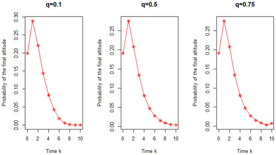
Figure 1. Simulation of the distribution of the final altitude $U_{10}$ with different values of $q=0.1,0.5$, and $0.75$.

Figure 2 shows that the probability of the final altitude $U_{50}$ is increasing from 0.1914062 for $k=0$ to attain its maximum 0.2758942 at $k=1$ for the three different values (0.1, 0.5, and 0.75) of $q_1$, starts decreasing and approach 0 at time $k=10$, respectively. Also, we observe that the decay rate of the density function of $U_{50}$ for $q_1=0.1$ is quicker than the others $q_1$ (0.5, and 0.75). Finally, we remark that the density function of $U_{50}$ equals 0 approximately from $k=25$ to $k=50$ for the three values 0.1, 0.5, and 0.75) of $q_1$. Plus, precisely, the probability $P(U_{50}=k)$ equals $8.809441\times {10}^{-7}$ and is decreasing to $1.846409\times {10}^{-14}$, $5.134722\times {10}^{-13}$, and $3.266140\times {10}^{-13}$ from time $k=25$ to 50 for the values (0.1, 0.5, and 0.75) of $q_1$, respectively.

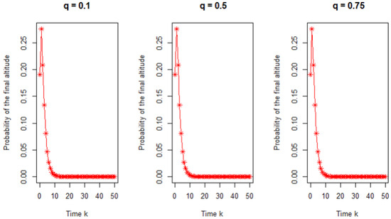
Figure 2. Simulation of the distribution of the final altitude $U_{50}$ with different values of $q=0.1,0.5$, and $0.75$.

From Figure 3, we observe that the probability of the final altitude $U_{100}$ is increasing from 0.1914062 for $k=0$ to attain its maximum 0.2758942 at $k=1$ for the three different values (0.1, 0.5, and 0.75) of $q_1$, starts decreasing and approach 0 at time $k=10$, respectively. Also, we observe that the decay rate of the density function of $U_{50}$ for $q_1=0.1$ is quicker than the others $q_1$ (0.5, and 0.75). Finally, we remark that the density function of $U_{100}$ equals 0 approximately from $k=25$ to $k=100$ for the three values 0.1, 0.5, and 0.75 of $q_1$. Plus, precisely, the probability $P(U_{100}=k)$ equals $8.809441\times {10}^{-7}$ and is decreasing to $4.960540\times {10}^{-28}$, $1.241540\times {10}^{-25}$, and $2.369189\times {10}^{-25}$ from time $k=25$ to 100, for the values (0.1, 0.5, and 0.75) of $q_1$, respectively.

Figure 3. Simulation of the distribution of the final altitude $U_{100}$ with different values of $q=0.1,0.5$, and $0.75$.

All the curves show that the distribution of the final altitude is primarily concentrated on small values, while the probability of taking large values tends to zero.

Table 1 lists the probability of the final altitude $U_n$, for $n=25$ with different values of $q_1$ (0.1, 0.5, and 0.75). In the first case, when the sequence $q_n$ starts from a small value equal to 0.1 at time 1 and increasing to 0.5625, which is the fixed point of the sequence $q_n$ defined in Equation (2), we remark that the probability of the random walk $Y_n$ is decreasing from 0.2758942 at time 1 to 0.2731112 at time 25. In the second case, when the sequence $q_n$ starts from a medium value equal to 0.5 at time 1 and increasing to 0.5625, we observe that the probability of the random walk $Y_n$ is decreasing from 0.2758942 at time 1 to $6.835509\times {10}^{-7}$ at time 25. In the last case, when the sequence $q_n$ starts from a high value equal to 0.75 at time 1 and increasing to 0.5625, we observe that the probability of the random walk $U_n$ is decreasing from 0.2758942 at time 1 to $1.304397\times {10}^{-6}$ at time 25. Also, we remark that the fixed point of the sequence $q_n$ in the first case is attained at the time 25 but in the second and third cases, it is attained at time 19.

Table 1. Computation of the probability distribution of the final altitude $Y_n$ for different values of $q_1$ (=0.1, 0.5, 0.75).

k	${\mathit{q}}_1=0.1$	$\mathit{P}({\mathit{U}}_{\mathit{n}}=\mathit{k})$	${\mathit{q}}_1=0.5$	$\mathit{P}({\mathit{U}}_{\mathit{n}}=\mathit{k})$	${\mathit{q}}_1=0.75$	$\mathit{P}({\mathit{U}}_{\mathit{n}}=\mathit{k})$
0	1.0000000	0.1985929	1.0000000	0.191448	1.0000000	0.1914062
1	0.1000000	2.758942e-01	0.5000000	0.2758942	0.7500000	0.2758942
2	0.1462500	0.2084190	0.5312500	0.2084189	0.6093750	0.2084189
3	0.2071266	0.1340775	0.5478516	0.1340774	0.5808105	0.1340774
4	0.2807338	$8.074750\times {10}^{-2}$	0.5558767	$8.074742\times {10}^{-2}$	0.5701756	$8.074742\times {10}^{-2}$
5	0.3598351	$4.710661\times {10}^{-2}$	0.5595585	$4.710651\times {10}^{-2}$	0.5657992	$4.710650\times {10}^{-2}$
6	0.4327611	$2.703102\times {10}^{-2}$	0.5612044	$2.703090\times {10}^{-2}$	0.5639325	$2.703090\times {10}^{-2}$
7	0.4889070	$1.537384\times {10}^{-2}$	0.5619315	$1.537368\times {10}^{-2}$	0.5631247	$1.537368\times {10}^{-2}$
8	0.5248872	$8.701309\times {10}^{-3}$	0.5622510	$8.701104\times {10}^{-3}$	0.5627729	$8.701101\times {10}^{-3}$
9	0.5446297	$4.911533\times {10}^{-3}$	0.5623910	$4.911271e\times {10}^{-3}$	0.5626193	$4.911268\times {10}^{-3}$
10	0.5543624	$2.768274\times {10}^{-3}$	0.5624523	$2.767938\times {10}^{-3}$	0.5625522	$2.767934\times {10}^{-3}$
11	0.5588736	$1.559089\times {10}^{-3}$	0.5624791	$1.558658\times {10}^{-3}$	0.5625228	$1.558653\times {10}^{-3}$
12	0.5609003	$8.778338\times {10}^{-4}$	0.5624909	$8.772823\times {10}^{-4}$	0.5625100	$8.772757\times {10}^{-4}$
13	0.5617976	$4.943445\times {10}^{-4}$	0.5624960	$4.936430\times {10}^{-4}$	0.5625044	$4.936344\times {10}^{-4}$
14	0.5621922	$2.786116\times {10}^{-4}$	0.5624983	$2.777307\times {10}^{-4}$	0.5625019	$2.777197\times {10}^{-4}$
15	0.5623652	$1.573182\times {10}^{-4}$	0.5624992	$1.562443\times {10}^{-4}$	0.5625008	$1.562302\times {10}^{-4}$
16	0.5624410	$8.912147\times {10}^{-5}$	0.5624997	$8.789762\times {10}^{-5}$	0.5625004	$8.787950\times {10}^{-5}$
17	0.5624742	$5.064433\times {10}^{-5}$	0.5624999	$4.945034\times {10}^{-5}$	0.5625002	$4.942704\times {10}^{-5}$
18	0.5624887	$2.859621\times {10}^{-5}$	0.5624999	$2.782433\times {10}^{-5}$	0.5625001	$2.779435\times {10}^{-5}$
19	0.5624951	$1.551693\times {10}^{-5}$	0.5625000	$1.566149\times {10}^{-5}$	0.5625000	$1.562291\times {10}^{-5}$
20	0.5624978	$7.578482\times {10}^{-6}$	0.5625000	$8.822321\times {10}^{-6}$	0.5625000	$8.772609\times {10}^{-6}$
21	0.5624991	$3.063972\times {10}^{-6}$	0.5625000	$4.977887\times {10}^{-6}$	0.5625000	$4.913523\times {10}^{-6}$
22	0.5624996	$9.481874\times {10}^{-7}$	0.5625000	$2.817098\times {10}^{-6}$	0.5625000	$2.732258\times {10}^{-6}$
23	0.5624998	$2.114740\times {10}^{-7}$	0.5625000	$1.600020\times {10}^{-6}$	0.5625000	$1.478789\times {10}^{-6}$
24	0.5624999	$3.260353\times {10}^{-8}$	0.5625000	$9.066788\times {10}^{-7}$	0.5625000	$5.767281\times {10}^{-7}$
25	0.5625000	$2.731112\times {10}^{-9}$	0.5625000	$6.835509\times {10}^{-7}$	0.5625000	$1.304397\times {10}^{-6}$

From Table 2, we remark that the mean of the final altitude is increasing from time 2 to time 34 for different values of $q_1=0.1$, 0.5, and 0.75 and is stable at any time n more than 34. Also, the maximum mean is attained at time 35 of the final altitude $U_n$ and equals 2.108571 for the three values of $q_1$. But the maximum variance is attained at time 40 of the final altitude $U_n$ and equals 3.846269 for the three values of $q_1$. In addition, it is stable at any time n greater than or equal to 40.

Table 2. Computation of the mean and the variance of the final altitude $U_n$ at different times n for different values of $q_1$ (=0.1, 0.5, and 0.75).

n	${\mathit{q}}_1=0.1$		${\mathit{q}}_1=0.5$		${\mathit{q}}_1=0.75$
	$\mathbb{E}\left({\mathit{U}}_{\mathit{n}}\right)$	$\mathbb{V}\mathbf{ar}\left({\mathit{U}}_{\mathit{n}}\right)$	$\mathbb{E}\left({\mathit{U}}_{\mathit{n}}\right)$	$\mathbb{V}\mathbf{ar}\left({\mathit{U}}_{\mathit{n}}\right)$	$\mathbb{E}\left({\mathit{U}}_{\mathit{n}}\right)$	$\mathbb{V}\mathbf{ar}\left({\mathit{U}}_{\mathit{n}}\right)$
2	0.2927267	0.2576897	0.8662724	0.6625369	0.7634247	0.801805
3	0.4340728	0.3831944	1.295987	1.156994	1.305294	1.484398
4	0.6128307	0.5369151	1.590949	1.671204	1.639145	2.073645
5	0.8294468	0.7295031	1.784657	2.163199	1.831367	2.561173
6	1.071507	0.9698979	1.908665	2.594731	1.942151	2.937289
7	1.315971	1.264419	1.986578	2.946729	2.007359	3.213559
8	1.537325	1.61087	2.034805	3.217844	2.046565	3.410965
9	1.71805	1.991955	2.064301	3.417481	2.070489	3.549767
10	1.853148	2.376771	2.082165	3.559369	2.085199	3.646234
15	2.087933	3.585933	2.106694	3.814743	2.106639	3.821841
20	2.107294	3.819183	2.108445	3.843417	2.108426	3.843783
25	2.108498	3.84401	2.108563	3.846037	2.108561	3.846046
30	2.108567	3.8461	2.108571	3.846252	2.108571	3.846251
35	2.108571	3.846258	2.108571	3.846268	2.108571	3.846268
40	2.108571	3.846269	2.108571	3.846269	2.108571	3.846269
45	2.108571	3.846269	2.108571	3.846269	2.108571	3.846269
50	2.108571	3.846269	2.108571	3.846269	2.108571	3.846269
100	2.108571	3.846269	2.108571	3.846269	2.108571	3.846269
500	2.108571	3.846269	2.108571	3.846269	2.108571	3.846269
1000	2.108571	3.846269	2.108571	3.846269	2.108571	3.846269

5. Marginal Distribution of ${\mathit{U}}_{\mathit{n}}^{\left(\mathit{i}\right)},\mathit{i}=\mathbf{1},\mathbf{2}$

In this section, we analyze the distribution of two random walks $U_n^{\left(1\right)}$ and $U_n^{\left(2\right)}$. Precisely, we find just a closed form of the distribution of $U_n^{\left(1\right)}$ and by a similar argument, we determine the expression of the distribution of $U_n^{\left(2\right)}$. We introduce, for $i=1,2$, the random walk $U_n^{\left(i\right)}$: for all $n\ge 0$, given $U_n^{\left(i\right)}$, the values of $U_{n+1}^{\left(i\right)}$ are given by

$$\begin{array}{c}\hfill U_{n+1}^{\left(i\right)}=\left\{\begin{array}{c}{U}_n^{\left(i\right)}+1,\mathrm{with}\mathrm{probability}{q}_{n+1},\hfill \\ \\ 0,\mathrm{with}\mathrm{probability}1-q_{n+1}.\hfill \end{array}\right.\end{array}$$

(4)

From System (4), we deduce the following lemma about the distribution of $U_n^{\left(1\right)}$ and by symmetries, we obtain also the distribution of $U_n^{\left(2\right)}$.

Lemma 1. 

For all $n\ge 1$, the distribution of $U_n^{\left(1\right)}$ is given by

$$\mathbb{P}(U_n^{\left(1\right)}=r)=\left\{\begin{array}{cc}{\displaystyle 1-q_n,}\hfill & ifr=0,\hfill \\ \\ {\displaystyle \prod _{r=1}^n{q}_r,}\hfill & ifr=n,\hfill \\ {\displaystyle (1-q_{n-r})\prod _{j=n+1-r}^n{q}_j,}\hfill & if0<r<n.\hfill \end{array}\right.$$

Proof. 

We start this proof the two special cases $k=0$ and $k=n$:

$$\mathbb{P}(U_n^{\left(1\right)}=0)=(1-q_n)\sum _{l=0}^{n-1}\mathbb{P}(U_{n-1}^{\left(1\right)}=l)=1-q_n,$$

$$\mathbb{P}(U_n^{\left(1\right)}=n)=q_n\mathbb{P}(U_{n-1}^{\left(1\right)}=n-1),$$

(5)

and we iterate Equation (5), then we obtain

$$\mathbb{P}(U_n^{\left(1\right)}=n)=q_n\mathbb{P}(U_{n-1}^{\left(1\right)}=n-1)=\prod _{r=1}^n{q}_r.$$

For $0<r<n$ we use recurrence reasoning. We take $n=2$ and $r=1$, and it is clear that

$$\mathbb{P}(U_2^{\left(1\right)}=1)=q_2\mathbb{P}(U_1^{\left(1\right)}=0)=q_2(1-q_1),$$

and supposing that

$$\mathbb{P}(U_n^{\left(1\right)}=r)=(1-q_{n-r})\prod _{j=n+1-r}^n{q}_j,$$

(6)

we prove that the preceding hypothesis is true for $n+1$

$$\mathbb{P}(U_{n+1}^{\left(1\right)}=r)=q_{n+1}\mathbb{P}(U_n^{\left(1\right)}=r-1),$$

using (6), then we obtain

$$\mathbb{P}(U_{n+1}^{\left(1\right)}=r)=q_{n+1}(1-q_{n+1-r})\prod _{j=n+2-r}^n{q}_j=(1-q_{n+1-r})\prod _{j=n+2-r}^{n+1}{q}_j,$$

and we finish the proof. □

Remark 2. 

By symmetry, we have that for all $n\ge 1$, the distribution of $U_n^{\left(2\right)}$ is given by

$$\left\{\begin{array}{c}{\displaystyle \mathbb{P}(U_n^{\left(2\right)}=0)=1-q_n,\mathbb{P}(U_n^{\left(2\right)}=n)=\prod _{s=1}^n{q}_s,}\hfill \\ {\displaystyle \mathbb{P}(U_n^{\left(2\right)}=s)=(1-q_{n-s})\prod _{j=n+1-s}^n{q}_j,if0<s<n.}\hfill \end{array}\right.$$

We observe that for $q_1<3/4$ and n big enough,

$$\mathbb{P}(U_n^{\left(1\right)}=n)=\mathbb{P}(U_n^{\left(2\right)}=n)\approx C{\left({\displaystyle \frac{9}{16}}\right)}^n,$$

where C a strictly positive constant.

6. Recursive Equations

In this section, we find a closed form of the probability of the process defined in (1), denoted by $\mathbb{P}(U_n^{\left(1\right)}=r,U_n^{\left(2\right)}=s)$ at the time n. Precisely, we find a relationship between $\mathbb{P}(U_n^{\left(1\right)}=r,U_n^{\left(2\right)}=s)$ and $\mathbb{P}(U_{n-1}^{\left(1\right)}=k_1,U_{n-1}^{\left(2\right)}=k_2)$, for all $0\le r,s\le n$, using the conditional probability. We study three cases for $(r,s)$, $(0,0)$, $(r,0)$ or $(r,s)$, where $r\ge 1$ and $s\ge 1$. We start by the following notation: for all r, $s\in \{0,\dots ,n\}$

$${\mathbb{P}}_n(r,s)=\mathbb{P}\left(U_n^{\left(1\right)}=r,Y_n^{\left(2\right)}=s\right).$$

(7)

We start this section with a very important theorem. It leads to finding a closed form of the probability ${\mathbb{P}}_n(r,s)$ for all $r,s\in \{0,\dots ,n\}$. This theorem is very important and will be used to prove the first result: Theorem 1 in Section 3.

Theorem 3. 

The joint probability distribution of $(U_n^{\left(1\right)},U_n^{\left(2\right)})$ is given by

$$\begin{array}{cc}\hfill {\mathbb{P}}_n(r,s)& =\left\{\begin{array}{cc}{\displaystyle (1-q_{n-s})(1-q_{n-r})\prod _{k=0}^{s-1}{q}_{n-k}^2\prod _{j=n-r+1}^{n-s}{q}_j,}\hfill & if1\le s<r<n\hfill \\ {\displaystyle (1-q_n)(1-q_{n-r})\prod _{j=n+1-r}^n{q}_j,}\hfill & if1\le r<n,s=0,\hfill \\ {\displaystyle {(1-q_n)}^2,}\hfill & ifr=0,s=0.\hfill \end{array}\right.\hfill \end{array}$$

Remark 3. 

By similarity, we have that for all $1\le s<n$ and $r=0$

$${\displaystyle {\mathbb{P}}_n(0,s)=(1-q_n)(1-q_{n-s})\prod _{j=n+1-s}^n{q}_{j}and{\mathbb{P}}_n(0,n)=(1-q_n)\prod _{j=1}^n{q}_j.}$$

When n is very large, we have the following estimation:

$${\mathbb{P}}_n(0,0)\approx {\left({\displaystyle \frac{7}{16}}\right)}^2.$$

We will need the following lemmas to prove Theorem 3.

Lemma 2. 

We have the following recursion: for all $n>1$,

$$\left\{\begin{array}{c}{\displaystyle {\mathbb{P}}_n(n,0)=(1-q_n)\prod _{j=1}^n{q}_j,}\hfill \\ {\displaystyle {\mathbb{P}}_n(r,0)=(1-q_n)(1-q_{n-r})\prod _{j=n+1-r}^n{q}_j,if1\le r<n.}\hfill \end{array}\right.$$

Proof. 

For $1\le r<n$ and $s=0$, we have

$$\begin{array}{ccc}\hfill {\mathbb{P}}_n(r,0)& =& {\displaystyle \sum _{k=0}^n\mathbb{P}(U_n^{\left(1\right)}=r,U_n^{\left(2\right)}=0,U_{n-1}^{\left(1\right)}=r-1,U_{n-1}^{\left(2\right)}=k)}\hfill \\ & =& {\displaystyle \sum _{k=0}^n\mathbb{P}(U_n^{\left(1\right)}=r,U_n^{\left(2\right)}=0|U_{n-1}^{\left(1\right)}=r-1,U_{n-1}^{\left(2\right)}=k)}\hfill \\ & & \times \mathbb{P}(U_{n-1}^{\left(1\right)}=r-1,U_{n-1}^{\left(2\right)}=k)\hfill \\ & =& {\displaystyle q_n(1-q_n)\sum _{k=0}^{n-1}{\mathbb{P}}_{n-1}(r-1,k)}\hfill \\ & =& {\displaystyle q_n(1-q_n)\mathbb{P}\left(U_{n-1}^{\left(1\right)}=r-1\right)}\hfill \end{array}$$

Applying Lemma 1, we obtain

$${\mathbb{P}}_n(r,0)=(1-q_n)(1-q_{n-r})\prod _{j=n-r+1}^n{q}_j.$$

For the special case $r=n$, we have

$$\begin{array}{cc}\hfill {\mathbb{P}}_n(n,0)=& q_n(1-q_n)\mathbb{P}(Y_{n-1}^{\left(1\right)}=n-1),\hfill \end{array}$$

and applying Lemma 1, we obtain

$$\begin{array}{cc}\hfill {\mathbb{P}}_n(n,0)=& {\displaystyle (1-q_n)\prod _{j=1}^n{q}_j,}\hfill \end{array}$$

and the proof is finished. □

Remark 4. 

By symmetry, we have the following recursion:

$$\left\{\begin{array}{c}{\displaystyle {\mathbb{P}}_n(0,n)=(1-q_n)\prod _{j=1}^n{q}_j,}\hfill \\ {\displaystyle {\mathbb{P}}_n(0,s)=(1-q_n)(1-q_{n-s})\prod _{j=n+1-s}^n{q}_j,if1\le s<n.}\hfill \end{array}\right.$$

Lemma 3. 

We have the following recursion: for all $n>1$, $r>0$ and $s>0$

$${\mathbb{P}}_n(r,s)=\left\{\begin{array}{cc}{\displaystyle (1-q_{n-s})(1-q_{n-r})\prod _{k=0}^{s-1}{q}_{n-k}^2\prod _{j=n-r+1}^{n-s}{q}_j,}\hfill & if1\le s<r<n\hfill \\ {\displaystyle (1-q_{n-s})\prod _{k=0}^{s-1}{q}_{n-k}^2\prod _{j=1}^{n-s}{q}_j,}\hfill & if1\le s<r=n,\hfill \\ {\displaystyle {(1-q_{n-r})}^2\prod _{j=n-r+1}^n{q}_j^2,}\hfill & if1\le s=r<n,\hfill \\ {\displaystyle \prod _{j=1}^n{q}_j^2,}\hfill & if1\le s=r=n.\hfill \end{array}\right.$$

Proof. 

It is clear that, for $1\le r=s=n$, we have

$${\displaystyle {\mathbb{P}}_n(n,n)=\prod _{j=0}^n{q}_j^2.}$$

(8)

For all integers r, c and n such that $1\le s=r<n$, we iterate ${\mathbb{P}}_n(r,r)$, r times

$${\mathbb{P}}_n(r,r)=q_n^2\dots q_{n-r+1}^2{\mathbb{P}}_{n-r}(0,0)={(1-q_{n-r})}^2\prod _{j=n-r+1}^n{q}_j^2$$

(9)

For all $r>s$, we have

$$\begin{array}{ccc}\hfill {\mathbb{P}}_n(r,s)& =& \mathbb{P}(U_n^{\left(1\right)}=r,U_n^{\left(2\right)}=s)\hfill \\ & =& \mathbb{P}(U_n^{\left(1\right)}=r,U_n^{\left(2\right)}=s,U_{n-1}^{\left(1\right)}=r-1,U_{n-1}^{\left(2\right)}=s-1)\hfill \\ & =& \mathbb{P}(U_n^{\left(1\right)}=r,U_n^{\left(2\right)}=s|U_{n-1}^{\left(1\right)}=r-1,U_{n-1}^{\left(2\right)}=s-1)\hfill \\ & & \times \mathbb{P}(U_{n-1}^{\left(1\right)}=s-1,U_{n-1}^{\left(1\right)}=s-1)\hfill \\ & =& q_n^2{\mathbb{P}}_{n-1}(r-1,s-1)\hfill \\ & =& {\mathbb{P}}_{n-s}(r-s,0)\prod _{k=0}^{s-1}{q}_{n-k}^2.\hfill \end{array}$$

Applying Lemma 1, we have

$${\mathbb{P}}_{n-s}(r-s,0)=\left\{\begin{array}{cc}{\displaystyle (1-q_{n-s})(1-q_{n-r})\prod _{j=n-r+1}^{n-s}{q}_j,}\hfill & \mathrm{if}1\le s<r<n,\hfill \\ {\displaystyle (1-q_{n-s})\prod _{j=1}^{n-s}{q}_j,}\hfill & \mathrm{if}1\le s<r=n.\hfill \end{array}\right.$$

(10)

Combining Equations (8)–(10), we finish the proof. □

We use the preceding Lemmas 2 and 3 to prove Theorem 3.

Proof. 

It is clear that, for $r=s=0$ we have

$${\mathbb{P}}_n(0,0)={(1-q_n)}^2\approx {\left({\displaystyle \frac{7}{16}}\right)}^2.$$

For the rest of the proof, we can deduce directly from Lemmas 2 and 3. □

Corollary 2. 

We have the following recursion: for all $n\ge 1$, $k\ge 1$

$${\mathbb{P}}_n(k,k)=\left\{\begin{array}{cc}{\displaystyle {(1-q_{n-k})}^2\prod _{j=n-k+1}^n{q}_j^2,}\hfill & if1\le k<n,\hfill \\ {\displaystyle \prod _{j=1}^n{q}_j^2,}\hfill & ifk=n.\hfill \end{array}\right.$$

Proof. 

The proof is deduced directly from Lemma 3. □

7. Proofs

In this section, we prove the results in Section 3. We use Lemmas 2 and 3 and Corollary 2 to prove Theorem 1. For the proof of Theorem 2, we use Lemma 4. We start to prove Theorem 1.

Proof. 

We have the following: for all $k\ge 1$ and $n\ge 1$

$$\mathbb{P}\left(U_n=k\right)=2{\mathbb{P}}_n\left(k,0\right)+2\sum _{l=1}^{k-1}{\mathbb{P}}_n\left(k,l\right)+{\mathbb{P}}_n\left(k,k\right),$$

applying Lemmas 2 and 3 and Corollary 2, for all $1\le k<n$

$$\begin{array}{cc}\hfill {\mathbb{P}}_n(k,0)=& {\displaystyle (1-q_n)(1-q_{n-k})\prod _{j=n+1-k}^n{q}_j,}\hfill \\ \hfill {\mathbb{P}}_n\left(k,l\right)=& {\displaystyle (1-q_{n-l})(1-q_{n-k})\prod _{j=0}^{l-1}{q}_{n-j}^2\prod _{j=n-k+1}^{n-l}{q}_j,}\hfill \\ \hfill {\mathbb{P}}_n\left(k,k\right)=& {\displaystyle {(1-q_{n-k})}^2\prod _{j=n-k+1}^n{q}_j^2,}\hfill \end{array}$$

we obtain

$$\begin{array}{cc}\hfill \mathbb{P}(Y_n=k)=& {\displaystyle 2(1-q_n)(1-q_{n-k})\prod _{j=n+1-k}^n{q}_j+{(1-q_{n-k})}^2\prod _{j=n-k+1}^n{q}_j^2}\hfill \\ \hfill & {\displaystyle +2\sum _{l=1}^{k-1}\left((1-q_{n-l})(1-q_{n-k})\prod _{j=0}^{l-1}{q}_{n-j}^2\prod _{j=n-k+1}^{n-l}{q}_j\right).}\hfill \end{array}$$

In the case $k=n$, using the following equalities in Lemmas 2, 3 and Corollary 2,

$$\begin{array}{cc}\hfill {\mathbb{P}}_n(n,0)=& {\displaystyle (1-q_n)\prod _{j=1}^n{q}_j,}\hfill \\ \hfill {\mathbb{P}}_n\left(n,l\right)=& {\displaystyle (1-q_{n-l})\prod _{j=0}^{l-1}{q}_{n-j}^2\prod _{j=1}^{n-l}{q}_j,}\hfill \\ \hfill {\mathbb{P}}_n\left(n,n\right)=& {\displaystyle \prod _{j=1}^n{q}_j^2,}\hfill \end{array}$$

then, we obtain

$$\begin{array}{cc}\hfill \mathbb{P}(U_n=n)=& {\displaystyle 2(1-q_n)\prod _{j=1}^n{q}_j+2\sum _{l=1}^{n-1}\left((1-q_{n-l})\prod _{j=0}^{l-1}{q}_{n-j}^2\prod _{j=1}^{n-l}{q}_j\right)+\prod _{j=1}^n{q}_j^2.}\hfill \end{array}$$

□

In the following, we prove Theorem 2. We introduce the following technical lemma concerning the relationship between $f_{n+1}\left(h\right)$, $f_n\left(h\right)$ and $f_{n-1}\left(h\right)$, for all $h\ge 0$, for all $n\ge 1$, where the probability $f_n\left(h\right)$ represents the distribution of the height of the first component $Y_n^{\left(1\right)}$.

Lemma 4. 

We have the following recursion, for all $n\ge 1$:

$$f_{n+1}\left(h\right)=f_n\left(h\right)-q_{n+1}{q}_n{f}_{n-1}\left(h\right).$$

Proof. 

We have, for all $h\ge 0$,

$$\begin{array}{cc}\hfill f_{n+1}\left(h\right)=& \mathbb{P}\left[U_0^{\left(1\right)}\le h,U_1^{\left(1\right)}\le h,\cdots ,U_{n+1}^{\left(1\right)}\le h\right]\hfill \\ \hfill =& \mathbb{E}\left[{\mathbb{I}}_{\{U_0^{\left(1\right)}\le h,U_1^{\left(1\right)}\le h,\cdots ,U_{n+1}^{\left(1\right)}\le h\}}\right]\hfill \\ \hfill =& \mathbb{E}\left[{\mathbb{I}}_{\{U_0^{\left(1\right)}\le h,U_1^{\left(1\right)}\le h,\cdots ,U_n^{\left(1\right)}\le h\}}{\mathbb{I}}_{\{U_{n+1}^{\left(1\right)}\le h\}}\right]\hfill \\ \hfill =& \mathbb{E}\left[{\mathbb{I}}_{\{U_0^{\left(1\right)}\le h,U_1^{\left(1\right)}\le h,\cdots ,U_n^{\left(1\right)}\le h\}}\left(1-{\mathbb{I}}_{\{U_{n+1}^{\left(1\right)}\ge h+1\}}\right)\right]\hfill \\ \hfill =& \mathbb{E}\left[{\mathbb{I}}_{\{U_0^{\left(1\right)}\le h,U_1^{\left(1\right)}\le h,\cdots ,U_n^{\left(1\right)}\le h\}}\right]-\mathbb{E}\left[{\mathbb{I}}_{\{U_0^{\left(1\right)}\le h,U_1^{\left(1\right)}\le h,\cdots ,U_n^{\left(1\right)}\le h\}}{\mathbb{I}}_{\{U_{n+1}^{\left(1\right)}\ge h+1\}}\right]\hfill \\ \hfill =& f_n\left(h\right)-\mathbb{P}\left[U_0^{\left(1\right)}\le h,U_1^{\left(1\right)}\le h,\cdots ,U_{n-1}^{\left(1\right)}\le h,U_n^{\left(1\right)}=h,U_{n+1}^{\left(1\right)}=h+1\right]\hfill \\ \hfill =& f_n\left(h\right)-\mathbb{P}\left(U_{n+1}^{\left(1\right)}=h+1|\{U_0^{\left(1\right)}\le h,U_1^{\left(1\right)}\le h,\cdots ,U_{n-1}^{\left(1\right)}\le h,U_n^{\left(1\right)}=h\}\right)\hfill \\ \hfill & \times \mathbb{P}\left(U_0^{\left(1\right)}\le h,U_1^{\left(1\right)}\le h,\cdots ,U_{n-1}^{\left(1\right)}\le h,U_n^{\left(1\right)}=h\right)\hfill \\ \hfill =& f_n\left(h\right)-\mathbb{P}\left(U_{n+1}^{\left(1\right)}=h+1|\{U_n^{\left(1\right)}=h\}\right)\times \mathbb{P}\left(U_n^{\left(1\right)}=h|\{U_{n-1}^{\left(1\right)}\le h\}\right)\hfill \\ \hfill & \times \mathbb{P}\left(U_0^{\left(1\right)}\le h,U_1^{\left(1\right)}\le h,\cdots ,U_{n-1}^{\left(1\right)}\le h\right)\hfill \\ \hfill =& f_n\left(h\right)-q_{n+1}{q}_n{f}_{n-1}\left(h\right).\hfill \end{array}$$

The last equality is due to the fact that, if

$$R_n\left(h\right)=\mathbb{P}\left(U_0^{\left(1\right)}\le h,U_1^{\left(1\right)}\le h,\cdots ,U_{n-1}^{\left(1\right)}\le h,U_n^{\left(1\right)}=h\right),$$

then

$$\begin{array}{cc}\hfill R_n\left(h\right)=& \mathbb{P}\left(U_n^{\left(1\right)}=h|\{U_0^{\left(1\right)}\le h,U_1^{\left(1\right)}\le h,\cdots ,U_{n-1}^{\left(1\right)}\le h\}\right)\times \mathbb{P}\left(U_0^{\left(1\right)}\le h,U_1^{\left(1\right)}\le h,\cdots ,U_{n-1}^{\left(1\right)}\le h\right)\hfill \\ \hfill =& \mathbb{P}\left(U_n^{\left(1\right)}=h|\{U_{n-1}^{\left(1\right)}\le h\}\right)\times f_{n-1}\left(h\right)\hfill \\ \hfill =& q_n\times f_{n-1}\left(h\right).\hfill \end{array}$$

□

Lemma 4 leads us to prove Theorem 2.

Proof. 

Denote, for all n by

$$A_n\left(h\right)=\left(\begin{array}{c}{f}_n\left(h\right)\\ f_{n-1}\left(h\right)\end{array}\right).$$

We have from Lemma 4,

$$A_n\left(h\right)=M_n\left(h\right)A_{n-1}\left(h\right),$$

then we obtain recursively

$$A_n\left(h\right)=\left[\prod _{l=2}^n{M}_l\left(h\right)\right]A_1\left(h\right)=N_n\left(h\right)A_1\left(h\right).$$

□

8. Conclusions and Perspective

In this work, we have introduced and analyzed a novel two-dimensional Moran walk model, characterized by a time-dependent probability distribution. Our main contributions include deriving explicit closed-form expressions for the probability distribution of the final maximum altitude, as well as providing a thorough statistical analysis of the model’s behavior through simulations and probabilistic techniques. These results shed new light on the statistical properties of the two-dimensional Moran process and contribute to a broader understanding of discrete stochastic processes in both mathematical and applied contexts. From a theoretical perspective, our findings highlight the significance of the transition probability dependence on time, which introduces additional complexity compared to traditional Moran processes. The obtained probability distribution functions, moment expressions, and cumulative distributions offer new insights into the extremal statistics of such stochastic processes. Furthermore, our simulations confirm the theoretical predictions and provide a deeper understanding of how different parameter choices affect the evolution of the Moran walk. As a perspective, several promising directions for future research emerge from our study:

• Extension to Higher Dimensions: While this work focuses on a two-dimensional setting, a natural extension would be to analyze the Moran walk in three or more dimensions. This generalization could provide a more comprehensive understanding of multidimensional population dynamics and other related stochastic processes.
• Derivation of Recurrence Relations: A key challenge is to establish explicit recurrence relations between the functions $f_n\left(u\right)$ and $f_{n+1}\left(u\right)$ that describe the evolution of height statistics. Extracting the coefficient $\left[z^n\right]F_{\le h}(z,1)$ would provide further insights into the distribution of $H_n$ and its limiting behavior.
• Asymptotic Analysis of Maximum Height: Determining the limiting behavior of $H_n$ as $n\to \infty$ would be an important theoretical advancement. This could be achieved through generating function techniques, kernel methods, and singularity analysis.
• Moment Generating Function for Height Statistics: Using moment generating functions, we could obtain refined information about the mean and variance of $H_n$. This approach would allow for a more comprehensive characterization of the distribution of the maximum altitude.
• Applications in Population Genetics and Evolutionary Biology: Given its origins in modeling genetic drift and allele frequency evolution, our Moran walk framework could be further adapted to incorporate selection effects, mutations, and varying population sizes. Such extensions would enhance the model’s applicability to real-world biological systems.
• Numerical Approximations and Machine Learning Approaches: The complexity of the recurrence relations and probability distributions suggests the potential benefit of employing numerical methods and machine learning techniques to approximate the behavior of the Moran walk under different parameter regimes.

Overall, this study provides a strong foundation for future explorations of time-dependent stochastic processes and their applications. We anticipate that the techniques developed here will prove valuable for both theoretical research and practical applications in various scientific fields.

References

- Moran, P.A.P. Random processes in genetics. Proc. Camb. Philos. Soc. 1958, 54, 60–71. [Google Scholar] [CrossRef]
- Moran, P.A.P. The Statistical Processes of Evolutionary Theory; Oxford University Press: Oxford, UK, 1962. [Google Scholar]
- Lieberman, E.; Hauert, C.; Nowak, M.A. Evolutionary dynamics on graphs. Nature 2005, 433, 312–316. [Google Scholar] [CrossRef] [PubMed]
- Banderier, C.; Flajolet, P. Basic analytic combinatorics of directed lattice paths. Theor. Comput. Sci. 2002, 281, 37–80. [Google Scholar] [CrossRef]
- Flajolet, P.; Sedgewick, R. Analytic Combinatorics; Cambridge University Press: Cambridge, UK, 2009. [Google Scholar]
- Flajolet, P.; Guillemin, F. The formal theory of birth-and-death processes, lattice path combinatorics and continued fractions. Adv. Appl. Probab. 2000, 32, 750–778. [Google Scholar] [CrossRef][Green Version]
- Drmota, M. Random Trees: An Interplay Between Combinatorics and Probability; Springer: Vienna, Austria, 2009. [Google Scholar]
- Abdelkader, M. On the Height of One-Dimensional Random Walk. Mathematics 2023, 11, 4513. [Google Scholar] [CrossRef]
- Banderier, C.; Nicodème, P. Bounded discrete walks. Discret. Math. Theor. Comput. Sci. 2010, AM, 35–48. [Google Scholar] [CrossRef]
- de Bruijn, N.G.; Knuth, D.E.; Rice, S.O. The average height of planted plane trees. In Graph Theory and Computing; Academic Press: Cambridge, MA, USA, 1972; pp. 15–22. [Google Scholar]
- Aguech, R.; Abdelkader, M. Two-Dimensional Moran Model: Final Altitude and Number of Resets. Mathematics 2023, 11, 3774. [Google Scholar] [CrossRef]
- Althagafi, A.; Abdelkader, M. Two-Dimensional Moran Model. Symmetry 2023, 15, 1046. [Google Scholar] [CrossRef]
- Huillet, T.E. Random walk Green kernels in the neutral Moran modelconditioned on survivors at a random time to origin. Math. Popul. Stud. 2016, 23, 164–200. [Google Scholar] [CrossRef]
- Huillet, T.; Möhle, M. Duality and asymptotics for a class of nonneutral discrete Moran models. J. Appl. Probab. 2009, 46, 866–893. [Google Scholar] [CrossRef][Green Version]
Disclaimer/Publisher’s Note: The statements, opinions and data contained in all publications are solely those of the individual author(s) and contributor(s) and not of MDPI and/or the editor(s). MDPI and/or the editor(s) disclaim responsibility for any injury to people or property resulting from any ideas, methods, instructions or products referred to in the content. |
© 2025 by the author. Licensee MDPI, Basel, Switzerland. This article is an open access article distributed under the terms and conditions of the Creative Commons Attribution (CC BY) license (https://creativecommons.org/licenses/by/4.0/).