Extracting Correlations in Arbitrary Diagonal Quantum States via Weak Couplings and Auxiliary Systems

Abstract

In this work, we introduce a novel method to extract correlations in diagonal quantum states in multi-particle quantum systems, addressing a significant limitation of traditional approaches that require prior knowledge of the density matrices of quantum states. Instead of relying on classical information processing, our method is based on weak couplings and ancillary systems, eliminating the need for classical communication, optimization, and complex calculations. The concept of mutually unbiased bases is intrinsically linked to symmetry, as it entails the uniform distribution of quantum states across distinct bases. Within the framework of our theoretical model, mutually unbiased bases are employed to facilitate weak measurements and to function as the post-selected states. To quantify the correlations in the initial state, we employ the trace distance between the initial state and the product of its marginal states, and illustrate the feasibility and effectiveness of our approach. We generalize the approach to accommodate high-dimensional multi-particle systems for potential applications in quantum information processing and quantum networks.

1. Introduction

Weak value was first proposed by Aharonov, Albert, and Vaidman in 1988 [1]. This technique is characterized by its minimal perturbation to the quantum system, allowing for the extraction of information from quantum states without inducing significant state collapse, as is the case with strong measurements. This unique feature has enabled the exploration of numerous novel physical phenomena and has led to extensive theoretical and experimental research in recent years. The applications of weak measurement have been widely investigated, including studies on the real and imaginary parts of weak values [2,3,4], the relationships between these parts, and measurement pointer parameters (such as mean position and mean momentum) [5,6,7,8]. Experimental realizations of weak measurement have also been demonstrated, with applications in various fields, including quantum correlations [9,10,11,12,13]. Specifically, weak measurement has been utilized in the distillation of entanglement, the variation in correlations under weak coupling, and the estimation of quantum states [14,15]. Weak measurement has enabled the achievement of several important physical goals, such as ultra-small polarization rotation measurements, the exploration of negative probabilities, and the enhancement of quantum teleportation fidelity through noisy channels [16,17,18].

Traditional ways to quantify correlations in a multipartite quantum system almost always start from a complete description of its density matrix. Whether one employs quantum-state tomography, entanglement witnesses, or more recent machine-learning-based estimators, the common premise is that at least one party must know the full set of density-matrix elements. This requirement becomes a critical bottleneck in realistic scenarios: the system may be prepared by a remote or untrusted device; its dimensionality may be too large for tomography to be practical; or the state may be encoded in fragile physical degrees of freedom that are destroyed by strong projective measurements [19,20,21].

Weak-value-based protocols have emerged as a promising alternative because they extract statistical information while imparting only a vanishingly small disturbance on the state. Pioneering experiments have already used weak measurements to estimate individual density-matrix elements, to distill entanglement, and even to perform full state tomography under restricted assumptions. However, these demonstrations still rely on prior knowledge of at least some entries of the density matrix, or they require classical communication among the parties to align measurement bases and post-process data. A framework that can quantify correlations in diagonal multipartite states without any prior information about the matrix elements, without classical communication between the parties, and without optimization loops has been missing. In this paper, we focus on the application of weak measurement in the realm of quantum correlations, aiming to develop a novel approach for extracting correlations from diagonal quantum states whose density-matrix expressions are unknown [22,23].

Symmetry is a fundamental concept in quantum mechanics, describing the invariance of a system under certain transformations. The concept of mutually unbiased bases is related to symmetry because it involves the uniform distribution of quantum states across different bases [24,25]. This uniform distribution can be regarded as a manifestation of symmetry, implying that transformations between different bases are symmetric, with no single basis being more special than the others. We utilize mutually unbiased bases as a fundamental tool acting as weak measurement operators and post-selected states.

To quantify the correlations in the initial state, we employ the trace distance between the initial state and the tensor product of its marginal states [26]. Quantum systems often interact with their environments [27,28,29], leading to complex dynamics influenced by initial correlations between the system and the environment. To quantify these correlations and their impact on system dynamics, the trace distance between a quantum state and its marginal product state has emerged as a powerful tool. This measure captures the total amount of correlations, including both classical and quantum contributions, and has been widely used to study non-Markovian processes and detect initial correlations through local measurements [30,31,32]. This model also leverages weak couplings [1,33], and incorporates auxiliary states [34] as a key component.

Previous methods for calculating trace distance have predominantly focused on scenarios where the density matrix of the quantum state is known [35,36,37,38,39,40]. The feasibility of employing the trace distance as a coherence measure for quantum states has been systematically investigated in Reference [36]. In this reference, diagonal states are utilized as incoherent states to quantify the coherence of a given state. In contrast, the present study focuses on diagonal states themselves, aiming to characterize the correlation content of arbitrary diagonal states.

This paper proposes a model for measuring trace distance in quantum states, even when the density-matrix expressions are not known in advance by the state owners, except that they are diagonal and their dimensions. After performing a series of operations according to the model, one of the owners can obtain correlations for the entire system, which consists of multiple particles. Each owner performs these operations individually, and no classical information is required during the intermediate steps.

The remainder of this paper is organized as follows. In Section 2, we describe our model for obtaining quantum correlations of states whose density-matrix expressions are not known. Section 2 is divided into three subsections. In Section 2.1, we explain weak measurements and their applications. In Section 2.2, we elaborate on our proposed model. In Section 2.3, we present key details of our model that are essential for its realization. In Section 3, we provide an example of a three-particle system in which our proposed model is applied. A discussion and summary are presented in Section 4.

2. Theoretical Model

This section begins with an introduction to the concepts of weak value and weak measurement, as well as a description of one of their applications, as presented in Reference [41]. It then proceeds with an introduction to our model and several key details that are crucial to its functioning.

2.1. Weak Measurement and Its Application

The concept of weak values in quantum mechanics was formulated by Aharonov, Albert, and Vaidman [1,33]. We consider an initial state $\left|{\psi }_{in}\right.〉$ and a final state $\left|{\psi }_{fin}\right.〉$, with $\left.〈{\psi }_{fin}\right|{\psi }_{in}〉\ne 0$. A measurement interaction between the system we investigate and the measuring device is $H_{\mathrm{int}}\left(t\right)=g\left(t\right)A{P}_d$. A is the measured observable in the system that we investigated. $P_d$ is canonically conjugate to an observable $Q_d$ representing the pointer position on the measuring device. The coupling $g\left(t\right)$ is non-zero for $0\le t\le T$ and is normalized such that ${\int }_0^{T}g\left(t\right)dt=g_0=1$ [42]. We choose $g\left(t\right)$ to be impulsive and assume that the time evolution operator for the measured system and the measuring device is $e^{-\left(i/\phantom{i\hslash }\hslash \right)A{P}_d}$. The measuring device is a quantum system and thus possesses a quantum state ${\varphi }_{in}\left(Q_d\right)$, then after the post-selection

$$\begin{array}{ccc}〈{\psi }_{fin}\left|e^{-\left(i/\phantom{i\hslash }\hslash \right)A{P}_d}\right|{\psi }_{in}〉{\varphi }_{in}\left(Q_d\right)\hfill & \approx & 〈{\psi }_{fin}\left|1-\left(i/\phantom{i\hslash }\hslash \right)A{P}_d\right|{\psi }_{in}〉{\varphi }_{in}\left(Q_d\right)\hfill \\ \hfill & =& 〈{\psi }_{fin}\left|\phantom{{\psi }_{fin}{\psi }_{in}}\right.{\psi }_{in}〉\left[1-\left(i/\phantom{i\hslash }\hslash \right){〈A〉}_w{P}_d\right]{\varphi }_{in}\left(Q_d\right)\hfill \\ \hfill & \approx & 〈{\psi }_{fin}\left|\phantom{{\psi }_{fin}{\psi }_{in}}\right.{\psi }_{in}〉e^{-\left(i/\phantom{i\hslash }\hslash \right){〈A〉}_w{P}_d}{\varphi }_{in}\left(Q_d\right)\hfill \end{array},$$

(1)

$P_d$ is conjugate to an observable $Q_d$ presenting the pointer position on the measuring device. Here ${〈A〉}_w$ is the weak value of A

$${〈A〉}_w={\displaystyle \frac{〈{\psi }_{fin}\left|A\right|{\psi }_{in}〉}{〈{\psi }_{fin}\left|\phantom{{\psi }_{fin}{\psi }_{in}}\right.{\psi }_{in}〉}}.$$

(2)

Consequently, the displacement of the pointer on the measuring device is

$${\varphi }_{fin}\left(Q_d\right)\approx e^{-\left(i/\phantom{i\hslash }\hslash \right){〈A〉}_w{P}_d}{\varphi }_{in}\left(Q_d\right)={\varphi }_{in}\left(Q_d-{〈A〉}_w\right).$$

(3)

The schematic of the weak-value protocol is shown in Figure 1.

There has been significant interest in the applications of weak values since their introduction [43,44], particularly in applications [41] that are utilized in our model. We consider a quantum state whose density matrix is unknown, except for its diagonality and dimensions. Our objective is to determine the correlations of this state. A complete set of projective operators $\left\{A_i\right\}=\{\left|a_i\right.〉\langle a_i\left|\right\}$ is employed to perform weak measurements, and a final projective measurement basis $\left\{\left|b_k\right.〉\right\}$ serves as the post-selected states. Similarly, the eigen-decomposition of operators is mentioned in Reference [45], where this work establishes the connection between the Kirkwood–Dirac(KD) distribution and measurable weak values, elevating the KD distribution from an abstract state representation to one that is experimentally significant and practical.

According to Equation (1), Equation (10) can be obtained. The derivation from Equation (1) to Equation (10) is originally based on Reference [44]. Here, we assume that there is no nonunitary evolution over time during the post-selection process and the weak measurement process. Thus, the derivation simplifies as follows. Let the density matrix of the mixed state be denoted by $\rho$, which can be expressed as a combination of pure states:

$$\rho ={\displaystyle \sum _n}{p}_n\left|{\psi }_n\right.〉\left.〈{\psi }_n\right|\left(p_n\ge 0,{\displaystyle \sum _n}{p}_n=1\right).$$

(4)

Here, $\left|{\psi }_n\right.〉$ represents the pure state components, and $p_n$ denotes their respective probability weights. For each pure state component $\left|{\psi }_n\right.〉$, its weak value is given by Equation (2),

$$A_{w,n}={\displaystyle \frac{〈{\psi }_{fin}\left|A\right|{\psi }_n〉}{〈{\psi }_{fin}\left|\phantom{{\psi }_{fin}{\psi }_n}\right.{\psi }_n〉}}.$$

(5)

The weighted probability corresponding to the weak value of each pure state is expressed as follows:

$$P_n={\displaystyle \frac{p_n{\left|〈{\psi }_{fin}\left|\phantom{{\psi }_{fin}{\psi }_n}\right.{\psi }_n〉\right|}^2}{{\displaystyle \sum _m}{p}_m{\left|〈{\psi }_{fin}\left|\phantom{{\psi }_{fin}{\psi }_m}\right.{\psi }_m〉\right|}^2}}.$$

(6)

The weak value of the mixed state is obtained by taking the weighted average of the weak values associated with all pure state components,

$$A_w={\displaystyle \sum _n}{P}_n{A}_{w,n}={\displaystyle \frac{{\displaystyle \sum _n}{p}_n{\left|〈{\psi }_{fin}\left|\phantom{{\psi }_{fin}{\psi }_n}\right.{\psi }_n〉\right|}^2\frac{〈{\psi }_{fin}\left|A\right|{\psi }_n〉}{〈{\psi }_{fin}\left|\phantom{{\psi }_{fin}{\psi }_n}\right.{\psi }_n〉}}{{\displaystyle \sum _m}{p}_m{\left|〈{\psi }_{fin}\left|\phantom{{\psi }_{fin}{\psi }_m}\right.{\psi }_m〉\right|}^2}},$$

(7)

$$A_w={\displaystyle \frac{{\displaystyle \sum _n}{p}_n〈{\psi }_{fin}\left|A\right|{\psi }_n〉〈{\psi }_n\left|\phantom{{\psi }_n{\psi }_{fin}}\right.{\psi }_{fin}〉}{{\displaystyle \sum _m}{p}_m{\left|〈{\psi }_{fin}\left|\phantom{{\psi }_{fin}{\psi }_m}\right.{\psi }_m〉\right|}^2}}={\displaystyle \frac{〈{\psi }_{fin}\left|A\rho \right|{\psi }_{fin}〉}{〈{\psi }_{fin}\left|\rho \right|{\psi }_{fin}〉}}.$$

(8)

When the post-selected state is the projective measurement basis, the weak value of the mixed state is expressed as follows:

$$A_w={\displaystyle \frac{tr\left\{\left(\left|b_k\right.〉\left.〈b_k\right|\right)A\rho \right\}}{tr\left\{\left(\left|b_k\right.〉\left.〈b_k\right|\right)\rho \right\}}}.$$

(9)

So the weak value of the measurement $\left\{A_i\right\}$ is

$$W_{ki}={\displaystyle \frac{tr\left\{\left(\left|b_k\right.〉\left.〈b_k\right|\right)\left(\left|a_i\right.〉\left.〈a_i\right|\right)\rho \right\}}{tr\left(\left|b_k\right.〉\left.〈b_k\right|\rho \right)}}={\displaystyle \frac{〈b_k\left|\phantom{b_k{a}_i}\right.a_i〉〈a_i\left|\rho \right|b_k〉}{〈b_k\left|\rho \right|b_k〉}}.$$

(10)

Equation (10) can be rewritten as

$${\displaystyle \frac{W_{ki}〈b_k\left|\rho \right|b_k〉}{〈b_k\left|\phantom{b_k{a}_i}\right.a_i〉}}=〈a_i\left|\rho \right|b_k〉,$$

(11)

$${\displaystyle \sum _k}{\displaystyle \frac{W_{ki}〈b_k\left|\rho \right|b_k〉〈b_k\left|\phantom{b_k{a}_j}\right.a_j〉}{〈b_k\left|\phantom{b_k{a}_i}\right.a_i〉}}={\displaystyle \sum _k}〈a_i\left|\rho \right|b_k〉〈b_k\left|\phantom{b_k{a}_j}\right.a_j〉=〈a_i\left|\rho \right|a_j〉.$$

(12)

Then, the matrix elements of $\rho$ can be expressed as

$$〈a_i\left|\rho \right|a_j〉={\displaystyle \sum _k}〈b_k\left|\rho \right|b_k〉{\displaystyle \frac{〈b_k\left|\phantom{b_k{a}_j}\right.a_j〉}{〈b_k\left|\phantom{b_k{a}_i}\right.a_i〉}}{W}_{ki}={\displaystyle \sum _k}{P}_k{\displaystyle \frac{{\beta }_{kj}}{{\beta }_{ki}}}{W}_{ki},$$

(13)

where $W_{ki}$ is the weak value of projective operator $\left|a_i\right.〉\left.〈a_i\right|$ with the system state post-selected by the basis $\left|b_k\right.〉\left.〈b_k\right|$.

2.2. Correlation Abstraction of Quantum States with Unknown Density Matrices (Diagonal Only)

Suppose a density matrix for quantum system composed of A, B, and C is given as $\rho ={\displaystyle \sum _n}{p}_n\left|{\psi }_n\right.〉\langle {\psi }_n|$, where $\left|{\psi }_n\right.〉$ is the pure state decomposition components. It is convenient to rewrite the density matrix in the form $\rho ={\displaystyle \sum _{ijk}}{\alpha }_{ijk}\left|i,j,k\right.〉\left.〈i,j,k\right|$. The auxiliary systems will be prepared in initial entangled states with dimensions $l_1$ and $l_2$: ${\left|+\right.〉}_{A_N,C_{N_1}}=\left(1/\phantom{1\sqrt{l}}\sqrt{l_1}\right){\displaystyle \sum _m}{\left|m\right.〉}_{A_N}{\left|m\right.〉}_{C_{N_1}}$ and ${\left|+\right.〉}_{B_N,C_{N_2}}=\left(1/\phantom{1\sqrt{l_2}}\sqrt{l_2}\right){\displaystyle \sum _m}{\left|m\right.〉}_{B_N}{\left|m\right.〉}_{C_{N2}}$.

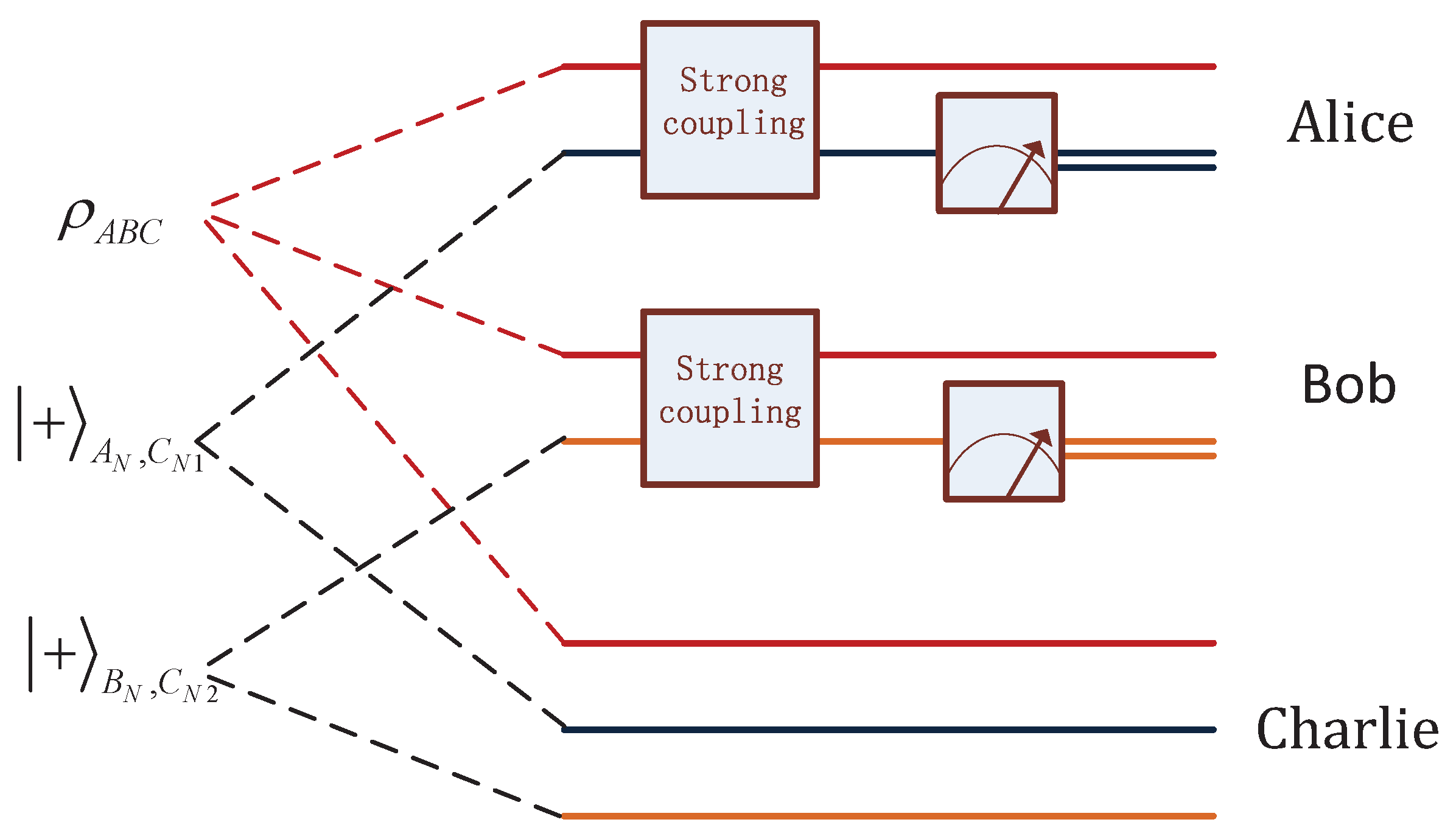
The dimensions of particles A and B, denoted as $l_1$ and $l_2$, respectively, may be either equal or distinct. In the quantum system, each particle is held by one of three distinct individuals: Alice, Bob, or Charlie. The three owners also possess corresponding auxiliary particles: $A_N$, $B_N$, $C_{N1}$, and $C_{N2}$, respectively. Within the domains controlled by Alice and Bob, system particles are coupled to their respective auxiliary particles. Specifically, particle A is strongly coupled to $A_N$ within Alice’s domain, while particle B is coupled to $B_N$ within Bob’s domain. Subsequently, local measurements are performed on the auxiliary particles. After the couplings are executed, Alice and Bob, respectively, measure the particles $A_N$ and $B_N$. The particles that have not been coupled and measured, namely C, $C_{N1}$, and $C_{N2}$, are all under the control of Charlie (see Figure 2). The primary purpose of the operations described above is to transfer the state of systems A, B, and C to the system of C, $C_{N1}$, and $C_{N2}$, which is denoted as ${\rho }_{C_{N1}{C}_{N2}C}$.

Charlie is tasked with characterizing the correlations within the system ${\rho }_{ABC}$. He continues to manipulate the particles $C_{N1}$, $C_{N2}$, and C (see Figure 3). The auxiliary systems ${\left|+\right.〉}_{{C^{\prime }}_{N1}{C^{″}}_{N1}}$, ${\left|+\right.〉}_{{C^{\prime }}_{N2}{C^{″}}_{N2}}$, and ${\left|+\right.〉}_{C^{\prime }{C}^{″}}$ are prepared in an entangled state and are strongly coupled to $C_{N1}$, $C_{N2}$, and C, respectively.

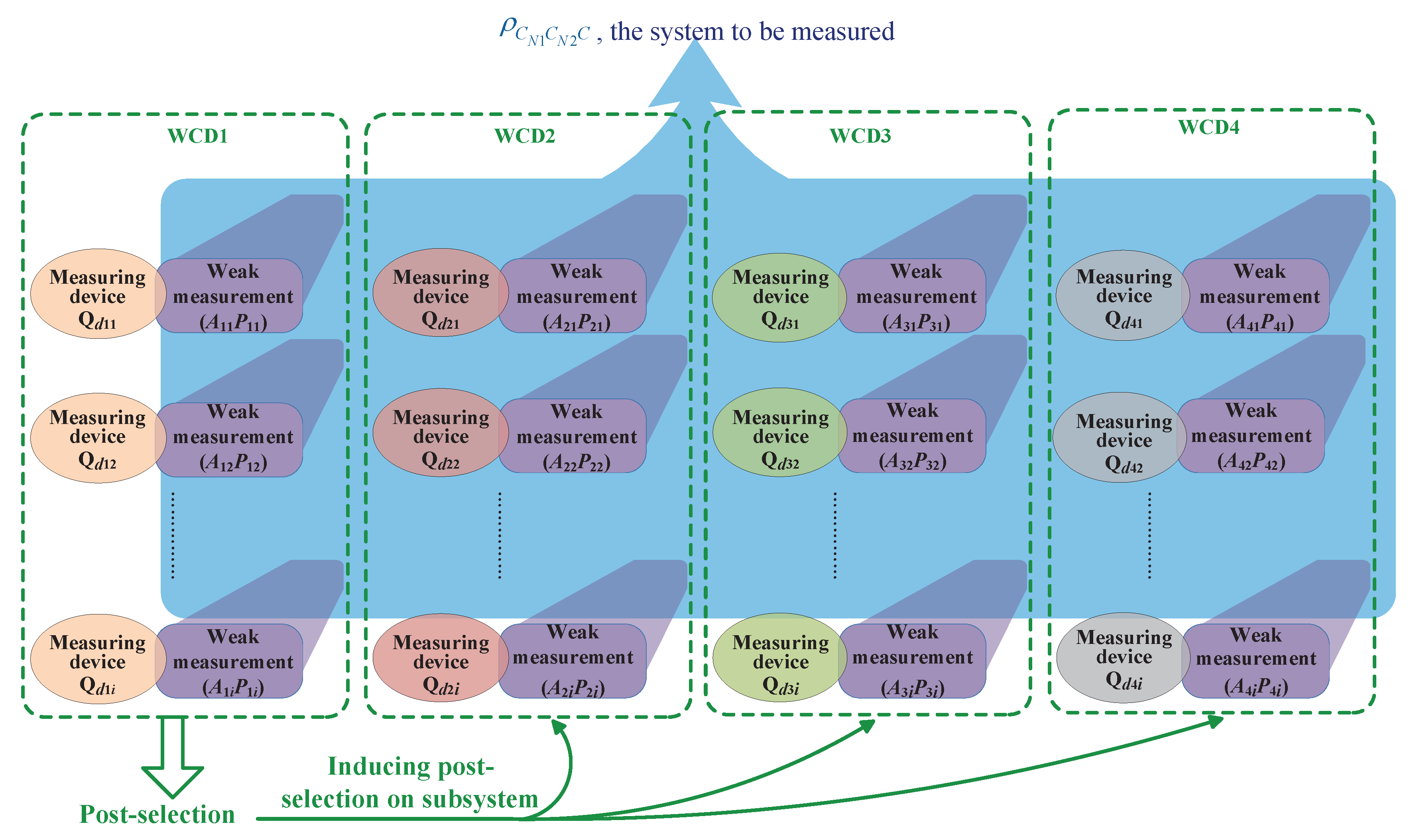
The weak-coupling device (WCD) consists of four operational lines: three auxiliary lines and one primary line designated as ${\rho }_{C_{N1}{C}_{N2}C}$. These lines are labeled WCD1, WCD2, WCD3, and WCD4. The ongoing operations are illustrated in Figure 4.

As shown in Figure 4, each weak coupling is associated with a measuring device that indicates the position and momentum displacements. These displacements are used to calculate the weak values of the measured operators [5]. The measuring devices in Figure 4 can be represented as a matrix.

For WCD1, $\left\{a_{11},a_{12},\dots a_{1i}\right\}$ forms the basis set of the system ${\rho }_{C_{N1}{C}_{N2}C}$, and $\{A_{11},A_{12},$$\dots A_{1i}\}=\left\{\left|a_{11}\right.〉\left.〈a_{11}\right|,\left|a_{12}\right.〉\left.〈a_{12}\right|,\dots \left|a_{1i}\right.〉\left.〈a_{1i}\right|\right\}$. In WCD2, $a_{2i}$ is an element of the basis set of the system ${\rho }_A$, selected from the same column of the weak-coupling device matrix as $a_{1i}$. Similarly, $a_{3i}$ and $a_{4i}$ are elements of the basis sets of ${\rho }_B$ and ${\rho }_C$, respectively. After completing all coupling operations, Charlie performs a post-selection operation on C, $C_{N1}$, and $C_{N2}$, causing the displacements of the pointers on the measuring devices.

$$W_{ki}={\displaystyle \frac{\mathrm{tr}\left\{\left(\left|b_k\right.〉\langle b_k|\right)\left(\left|a_{ji}\right.〉\langle a_{ji}|\right)\rho \right\}}{\mathrm{tr}\left\{\left(\left|b_k\right.〉\langle b_k|\right)\rho \right\}}},$$

(14)

where if $j=1$ the information of the whole system are abstracted, and the subsystem’s information is abstracted if $j=2,3,4$. $\left\{b_1,b_2,\dots b_k\right\}$ is a base set that is mutually unbiased to $\left\{a_{11},a_{12},\dots a_{1i}\right\}$.

$${\lambda }_i=\sum _{k=1}^n{P}_k\left[\epsilon \left({\varphi }_{fin}\left(Q_{d1i}\right)\right)-\prod _{j=2}^4\epsilon \left({\varphi }_{fin}\left(Q_{dji}\right)\right)\right],$$

(15)

where n represents the dimension of the quantum state ${\rho }_{ABC}$, and $\epsilon$ represents the process

$$\epsilon \left({\varphi }_{fin}\left(Q_d\right)\right):{\varphi }_{fin}\left(Q_d\right)\to {\varphi }_{in}\left(Q_d-W_{ki}\right)\to W_{ki}\to 〈a_{ji}\left|\rho \right|a_{ji}〉$$

(16)

by which the density matrices are derived from the pointer displacements (average position displacement and average momentum displacement, see Equation (17)) of the measuring devices, denoted by $Q_{d_{ji}}$, for a given value of k.

$$\mathrm{Re}\left(W_{ji}\right)={\displaystyle \frac{1}{g}}\delta q_{ji},\mathrm{Im}\left(W_{ji}\right)={\displaystyle \frac{1}{2{\left(\Delta p_{ji}\right)}^{2}g}}\delta p_{ji}.$$

(17)

$$D=-{\displaystyle \frac{1}{2}}\sum _{i=1({\lambda }_i<0)}^n{\lambda }_i,$$

(18)

The summation of the negative eigenvalues $\lambda$ in Equation (18) is performed to calculate the trace distance between the quantum state ${\rho }_{ABC}$ and the product of the individual quantum states of subsystems A, B, and C. Equation (15) does not account for the inner product between the two basis sets denoted by ${\beta }_{kj}$ or ${\beta }_{ki}$, as included in Equation (13). This is because the set $\left\{b_1,b_2,\dots b_k\right\}$ is mutually unbiased with respect to the set $\left\{a_{11},a_{12},\dots a_{1i}\right\}$, and the inner products with all basis states have the same magnitude or differ only by a phase. In particular, here we consider only diagonal quantum states, so that the subscripts of $\beta$ in Equation (13) are identical [24,25]. This symmetry implies that transformations between bases are unbiased. Consequently, we can omit the terms ${\beta }_{kj}$ and ${\beta }_{ki}$ in Equation (13), thereby enhancing the feasibility of our approach.

2.3. Some Details

The model presented in this paper employs the concept of trace distance [26]. The trace distance between the whole system ${\rho }_{ABC}$ and the product of the separable systems ${\rho }_A\otimes {\rho }_B\otimes {\rho }_C$ serves as a measure of the correlations in ${\rho }_{ABC}$ at a certain level.

If the two states commute they are diagonal in the same basis:

$$\rho ={\displaystyle \sum _i}{r}_i\left|i\right.〉\left.〈i\right|;\sigma ={\displaystyle \sum _i}{s}_i\left|i\right.〉\left.〈i\right|,$$

(19)

where as per usual we define $\left|A\right|=\sqrt{A^{†}A}.$ In this case, the trace distance between $\rho$ and $\sigma$ is as follows:

$$D_{(\rho ,\sigma )}={\displaystyle \frac{1}{2}}\mathrm{tr}\left|{\displaystyle \sum _i}\left(r_i-s_i\right)\left|i\right.〉\left.〈i\right|\right|,$$

(20)

which is the theoretical support for our model and manipulation Equation (15).

When the post-selection occurs in WCD1 on C, $C_{N1}$, and $C_{N2}$, the system particles in WCD2, WCD3, and WCD4 collapse to the post-selected state in WCD1 simultaneously. The displacements of the pointers in the four-line devices, as shown in Figure 4, including both position and momentum displacements, can be read out simultaneously. Thus the post-selection in WCD1 is the only post-selected operation required for the model presented in this paper.

Suppose that ${\mu }_1$ and ${\mu }_2$ are the values derived from the strong measurement meters shown in Figure 2. For ${\mu }_1=0$ and ${\mu }_2=0$, the desired result is achieved, yielding ${\rho }_{C_{N1}{C}_{N2}C}={\rho }_{ABC}$, given the desired outcome. For ${\mu }_1\ne 0$ or ${\mu }_2\ne 0$, the resulting state has the same spectrum as ${\rho }_{ABC}$. Therefore, the system’s correlations remain invariant with variations in $\mu$, as indicated by Equation (15). That is, if the control particle equals to 1, controlled-NOT(CNOT) unitary operations are performed on the target particle.

$$U_{c=1}=\left(\begin{array}{cc}0& 1\\ 1& 0\end{array}\right);\rho =\left(\begin{array}{cc}a& b\\ c& d\end{array}\right)$$

(21)

$$U_{c=1}^{†}\rho U_{c=1}=\left(\begin{array}{cc}0& 1\\ 1& 0\end{array}\right)\left(\begin{array}{cc}a& b\\ c& d\end{array}\right)\left(\begin{array}{cc}0& 1\\ 1& 0\end{array}\right)=\left(\begin{array}{cc}d& c\\ b& a\end{array}\right).$$

(22)

If $\rho$ is diagonal, as in the scenario presented in this article, these unitary operations do not change the fact that the quantum state matrix remains diagonal. These operations are confined to the subspace of individual particles.

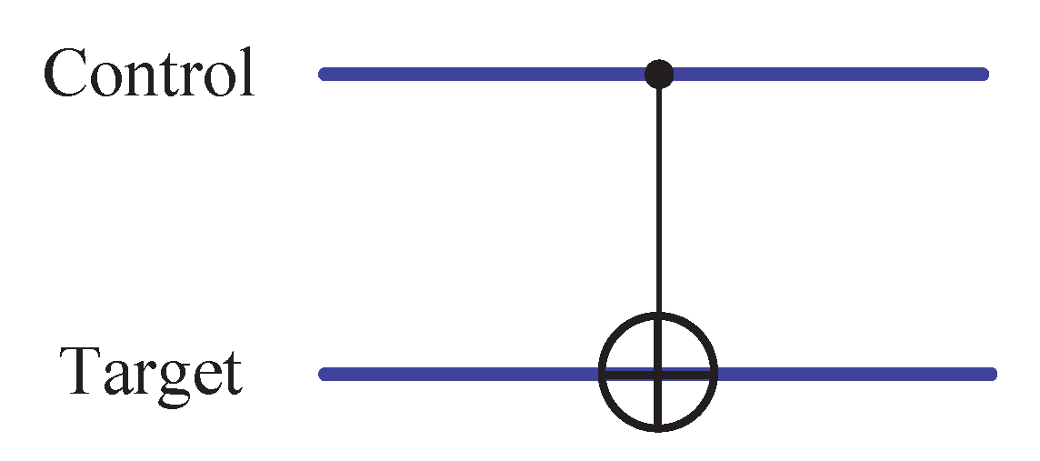
The controlled-NOT(CNOT) gate is the prototypical controlled operation in quantum computing. Expressed in the computational basis, the action of CNOT gate is given by $\left|c\right.〉\left|t\right.〉\to \left|c\right.〉\left|t\oplus c\right.〉$. That is, if the control qubit is set to $\left|1\right.〉$ then the target qubit is flipped, otherwise the target qubit is left alone. Thus, in the computational basis $\left|control,target\right.〉$ the matrix representation of CNOT is as follows:

$$\left(\begin{array}{cccc}1& 0& 0& 0\\ 0& 1& 0& 0\\ 0& 0& 0& 1\\ 0& 0& 1& 0\end{array}\right)$$

(23)

The circuit representation of CNOT is shown in Figure 5.

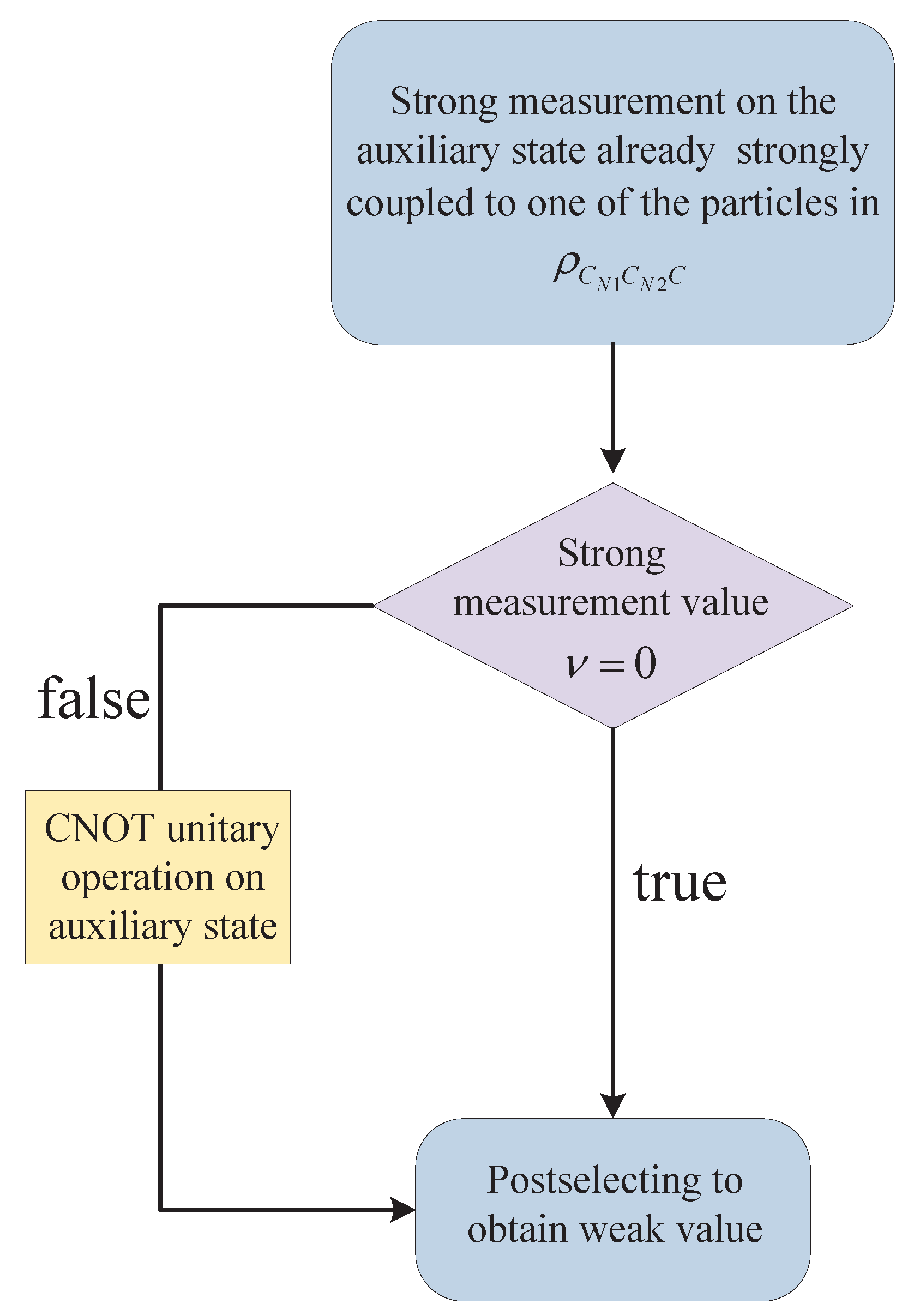
Assume that ${\nu }_1$, ${\nu }_2$, and ${\nu }_3$ are strong measurement readings depicted in Figure 3. The desired outcomes are ${\nu }_1=0$, ${\nu }_2=0$, and ${\nu }_3=0$. If ${\nu }_1\ne 0$, ${\nu }_2\ne 0$, or ${\nu }_3\ne 0$, a CNOT unitary operation should be applied (prior to weak measurement) on the subsystems in WCD2, WCD3, and WCD4 to ensure that the trace distance between the states ${\rho }_{ABC}$ and ${\rho }_A\otimes {\rho }_B\otimes {\rho }_C$ remain unchanged in such cases(see Figure 6). Here, CNOT unitary operations are performed on the subsystems with the control qubit set to $\left|1\right.〉$.

3. Example Implementations

We now provide an illustration concerning a quantum system ${\rho }_{ABC}$, which consists of three two-dimensional particles. Further elaboration on this will be provided in this section. Alice, Bob, and Charlie individually possess particles A, B, and C, respectively. They are unaware of any information about the system beyond its dimensionality and the basis set. Two bipartite maximally entangled states are prepared for use as auxiliary systems, named ${\left|+\right.〉}_{A_N,C_{N1}}$ and ${\left|+\right.〉}_{B_N,C_{N2}}$. Alice owns the first particle of ${\left|+\right.〉}_{A_N,C_{N1}}$, which is $A_N$, and Bob owns the first particle of ${\left|+\right.〉}_{B_N,C_{N2}}$, which is $B_N$. Charlie has $C_{N1}$ and $C_{N2}$ at his disposal. These two auxiliary states can be ${\displaystyle \frac{1}{\sqrt{2}}}\left(\left|00\right.〉+\left|11\right.〉\right)$ or ${\displaystyle \frac{1}{\sqrt{2}}}\left(\left|01\right.〉+\left|10\right.〉\right)$, both of which function equivalently. Particles A and B are, respectively, strongly coupled to their auxiliary system’s particles $A_N$ and $B_N$ by Alice and Bob. The strong couplings can be realized using a CNOT gate between the system particle and one of the auxiliary particles. Specifically, particle A is coupled to one of the particles within the state ${\displaystyle \frac{1}{\sqrt{2}}}\left(\left|00\right.〉+\left|11\right.〉\right)$, and particle B is coupled in the same manner. Subsequently, Alice and Bob perform strong measurements on particles $A_N$ and $B_N$, respectively. These measurements convert the quantum states of the particles into classical bits and induce a transition of the quantum state from ${\rho }_{ABC}$ to ${\rho }_{C_{N1}{C}_{N2}C}$. The measurements are realized by projecting onto the basis state $\left|0\right.〉$, as executed by both Alice and Bob. The outcome of these measurements implies that ${\rho }_{ABC}$ is equivalent to ${\rho }_{C_{N1}{C}_{N2}C}$. If the projection bases applied to the auxiliary systems are not $\left|0\right.〉$, the resulting state ${\rho }_{C_{N1}{C}_{N2}C}$ represents the effects of local operations on ${\rho }_{ABC}$, and such operations do not alter the final correlations derived from this model.

Charlie continues to work with the density matrix ${\rho }_{C_{N1}{C}_{N2}C}$, which is at his disposal. Initially, he prepares three auxiliary systems, coupling $C_{N1}$, $C_{N2}$, and C to them. The auxiliary systems ${\left|+\right.〉}_{C_{N1}^{\prime }{C}_{N1}^{″}}$, ${\left|+\right.〉}_{C_{N2}^{\prime }{C}_{N2}^{″}}$, and ${\left|+\right.〉}_{C^{\prime }{C}^{″}}$ can also be represented as ${\displaystyle \frac{1}{\sqrt{2}}}\left(\left|00\right.〉+\left|11\right.〉\right)$, as depicted in Figure 3. A base state $\left|0\right.〉$ is projected onto one of the two particles within the system ${\left|+\right.〉}_{C_{N1}^{\prime }{C}_{N1}^{″}}$ to complete a measurement on ${C^{″}}_{N1}$. This process yields the result that ${C^{″}}_{N1}$ is in the same quantum state as $C_{N1}$. A similar process is applied to $C_{N2}$ and C, with $C_{N2}^{\prime }$ and $C^{\prime }$, respectively, taking the state.

In the subsequent step, Charlie performs weak measurements on the four lines emanating from ${\rho }_{C_{N1}{C}_{N2}C}$ as shown in Figure 3. The weak measurement operators $A_{ji}$, depicted in Figure 4, are detailed in

Table 1. Weak measured operators in Figure 3. $A_{1i}$, $A_{2i}$, $A_{3i}$ and $A_{4i}$ are the weak measured observable operators. All operators are displayed in this table. $\left\{A_{11},A_{12},\dots A_{1i}\right\}$ is the base set of system ${\rho }_{C_{N1}{C}_{N2}C}$. The $A_{2i}$ is the element of the base set for the system ${\rho }_A$ picked out from $A_{1i}$ that is in the same column of weak couplings device matrix, and $A_{3i}$ and $A_{4i}$ are arranged in the same way which belong to the base set of ${\rho }_B$ and ${\rho }_C$.

i	1	2	3	4	5	6	7	8
$A_{1i}$	$\left|000\right.〉\left.〈000\right|$	$\left|001\right.〉\left.〈001\right|$	$\left|010\right.〉\left.〈010\right|$	$\left|011\right.〉\left.〈011\right|$	$\left|100\right.〉\left.〈100\right|$	$\left|101\right.〉\left.〈101\right|$	$\left|110\right.〉\left.〈110\right|$	$\left|111\right.〉\left.〈111\right|$
$A_{2i}$	$\left|0\right.〉\left.〈0\right|$	$\left|0\right.〉\left.〈0\right|$	$\left|0\right.〉\left.〈0\right|$	$\left|0\right.〉\left.〈0\right|$	$\left|1\right.〉\left.〈1\right|$	$\left|1\right.〉\left.〈1\right|$	$\left|1\right.〉\left.〈1\right|$	$\left|1\right.〉\left.〈1\right|$
$A_{3i}$	$\left|0\right.〉\left.〈0\right|$	$\left|0\right.〉\left.〈0\right|$	$\left|1\right.〉\left.〈1\right|$	$\left|1\right.〉\left.〈1\right|$	$\left|0\right.〉\left.〈0\right|$	$\left|0\right.〉\left.〈0\right|$	$\left|1\right.〉\left.〈1\right|$	$\left|1\right.〉\left.〈1\right|$
$A_{4i}$	$\left|0\right.〉\left.〈0\right|$	$\left|1\right.〉\left.〈1\right|$	$\left|0\right.〉\left.〈0\right|$	$\left|1\right.〉\left.〈1\right|$	$\left|0\right.〉\left.〈0\right|$	$\left|1\right.〉\left.〈1\right|$	$\left|0\right.〉\left.〈0\right|$	$\left|1\right.〉\left.〈1\right|$

. The pointer devices $Q_{d_{ji}}$ enable us to read the average position displacement $\delta q_{ji}$ and the average momentum displacement $\delta p_{ji}$. These displacements, induced by post-selection, allow us to calculate the weak values.

Equation (15) gives the necessity of considering each element of the base set acting as post-selected states, and this base set is mutually unbiased with respect to the base set of the system whose correlation we aim to obtain. All post-selected states are presented in

Table 2. The post-selected states. $\left\{b_1,b_2,\dots b_k\right\}$ is a base set that is mutually unbiased to $\left\{a_{11},a_{12},\dots a_{1i}\right\}$. $\left\{a_{11},a_{12},\dots a_{1i}\right\}$ is the base set of the system whose correlation we aim to obtain. Here, coefficient ${\displaystyle \frac{1}{\sqrt{8}}}$ is omitted for simplicity.

k	${\mathit{b}}_{\mathit{k}}$
1	$\left|000\right.〉+\left|001\right.〉+\left|010\right.〉+\left|011\right.〉+\left|100\right.〉+\left|101\right.〉+\left|110\right.〉+\left|111\right.〉$
2	$\left|000\right.〉-\left|001\right.〉+\left|010\right.〉-\left|011\right.〉+\left|100\right.〉-\left|101\right.〉+\left|110\right.〉-\left|111\right.〉$
3	$\left|000\right.〉+\left|001\right.〉-\left|010\right.〉-\left|011\right.〉+\left|100\right.〉+\left|101\right.〉-\left|110\right.〉-\left|111\right.〉$
4	$\left|000\right.〉-\left|001\right.〉-\left|010\right.〉+\left|011\right.〉+\left|100\right.〉-\left|101\right.〉-\left|110\right.〉+\left|111\right.〉$
5	$\left|000\right.〉+\left|001\right.〉+\left|010\right.〉+\left|011\right.〉-\left|100\right.〉-\left|101\right.〉-\left|110\right.〉-\left|111\right.〉$
6	$\left|000\right.〉-\left|001\right.〉+\left|010\right.〉-\left|011\right.〉-\left|100\right.〉+\left|101\right.〉-\left|110\right.〉+\left|111\right.〉$
7	$\left|000\right.〉+\left|001\right.〉-\left|010\right.〉-\left|011\right.〉-\left|100\right.〉-\left|101\right.〉+\left|110\right.〉+\left|111\right.〉$
8	$\left|000\right.〉-\left|001\right.〉-\left|010\right.〉+\left|011\right.〉-\left|100\right.〉+\left|101\right.〉+\left|110\right.〉-\left|111\right.〉$

.

For illustration, we consider a three-particle quantum state in two-dimensional space, of which the quantum density matrix ${\rho }_{ABC}={\displaystyle \frac{p}{8}}\left|000\right.〉\left.〈000\right|+{\displaystyle \frac{3p}{8}}\left|001\right.〉\left.〈001\right|+{\displaystyle \frac{p}{2}}\left|010\right.〉\left.〈010\right|+{\displaystyle \frac{1-p}{5}}\left|011\right.〉$ $\left.〈011\right|+{\displaystyle \frac{1-p}{5}}\left|100\right.〉\left.〈100\right|+{\displaystyle \frac{1-p}{5}}\left|101\right.〉\left.〈101\right|+{\displaystyle \frac{1-p}{5}}\left|110\right.〉\left.〈110\right|+{\displaystyle \frac{1-p}{5}}\left|111\right.〉\left.〈111\right|$. We do not have any information about this quantum state, including quantum density matrix.

One of the particles in the auxiliary system ${\displaystyle \frac{1}{\sqrt{2}}}\left(\left|00\right.〉+\left|11\right.〉\right)$ is strongly coupled to particle A in ${\rho }_{ABC}$ by Alice, and one of the particles in another auxiliary system ${\displaystyle \frac{1}{\sqrt{2}}}\left(\left|00\right.〉+\left|11\right.〉\right)$ is strongly coupled to particle B in ${\rho }_{ABC}$ by Bob. Then, Alice and Bob measure the coupled particles in the auxiliary systems using the basis vector $\left|0\right.〉$. Following these operations, the density matrix of the system composed of C and two uncoupled particles in the auxiliary systems is ${\rho }_{C{C}_{N1}{C}_{N2}}$. The difference between ${\rho }_{C{C}_{N1}{C}_{N2}}$ and ${\rho }_{ABC}$ is only a normalization constant, which is induced by measuring the auxiliary systems with $\left|0\right.〉$.

$${\rho }_{C{C}_{N1}{C}_{N2}}=\left(\begin{array}{cccccccc}{\displaystyle \frac{p}{32}}& 0& 0& 0& 0& 0& 0& 0\\ 0& {\displaystyle \frac{p}{8}}& 0& 0& 0& 0& 0& 0\\ 0& 0& {\displaystyle \frac{1-p}{20}}& 0& 0& 0& 0& 0\\ 0& 0& 0& {\displaystyle \frac{1-p}{20}}& 0& 0& 0& 0\\ 0& 0& 0& 0& {\displaystyle \frac{3p}{32}}& 0& 0& 0\\ 0& 0& 0& 0& 0& {\displaystyle \frac{1-p}{20}}& 0& 0\\ 0& 0& 0& 0& 0& 0& {\displaystyle \frac{1-p}{20}}& 0\\ 0& 0& 0& 0& 0& 0& 0& {\displaystyle \frac{1-p}{20}}\end{array}\right).$$

(24)

$${\rho }_{ABC}=\left(\begin{array}{cccccccc}{\displaystyle \frac{p}{8}}& 0& 0& 0& 0& 0& 0& 0\\ 0& {\displaystyle \frac{3p}{8}}& 0& 0& 0& 0& 0& 0\\ 0& 0& {\displaystyle \frac{p}{2}}& 0& 0& 0& 0& 0\\ 0& 0& 0& {\displaystyle \frac{1-p}{5}}& 0& 0& 0& 0\\ 0& 0& 0& 0& {\displaystyle \frac{1-p}{5}}& 0& 0& 0\\ 0& 0& 0& 0& 0& {\displaystyle \frac{1-p}{5}}& 0& 0\\ 0& 0& 0& 0& 0& 0& {\displaystyle \frac{1-p}{5}}& 0\\ 0& 0& 0& 0& 0& 0& 0& {\displaystyle \frac{1-p}{5}}\end{array}\right).$$

(25)

To acquire information about the subsystem, Charlie implements a strong coupling between the first particle of the system, which is composed of C, $C_{N1}$, and $C_{N2}$, and a particle in the auxiliary system denoted as ${C^{\prime }}_{N1}$. A subsequent measurement is conducted.

If Charlie measures the strongly coupled particle in the auxiliary system in the basis state $\left|1\right.〉$ and is successful, the state of the auxiliary system can be represented by the density matrix

$${\rho }_{C_{N1}^{″}}=\left(\begin{array}{cc}{\displaystyle \frac{2}{5}}+{\displaystyle \frac{9p}{40}}& 0\\ 0& {\displaystyle \frac{3}{5}}-{\displaystyle \frac{9p}{40}}\end{array}\right).$$

(26)

To obtain the density matrix of particle C, Charlie implements a unitary operation on particle ${C^{″}}_{N1}$, and the process is illustrated as follows:

$$\begin{array}{c}U{\rho }_{C_{N1}^{″}}{U}^{†}=\left(\begin{array}{cc}0& 1\\ 1& 0\end{array}\right).\left(\begin{array}{cc}{\displaystyle \frac{3}{80}}\left(8-3p\right)& 0\\ 0& {\displaystyle \frac{1}{5}}+{\displaystyle \frac{9p}{80}}\end{array}\right).\left(\begin{array}{cc}0& 1\\ 1& 0\end{array}\right)\\ \\ =\left(\begin{array}{cc}{\displaystyle \frac{1}{5}}+{\displaystyle \frac{9p}{80}}& 0\\ 0& {\displaystyle \frac{3}{80}}\left(8-3p\right)\end{array}\right)=2{\rho }_C.\end{array}$$

(27)

The unitary operator is derived from the measurement using the basis state $\left|1\right.〉$. When the basis state is $\left|0\right.〉$, the density matrix of ${C^{″}}_{N1}$ is identical to that of particle C. This method can be employed by Charlie to extract information from the other two subsystems.

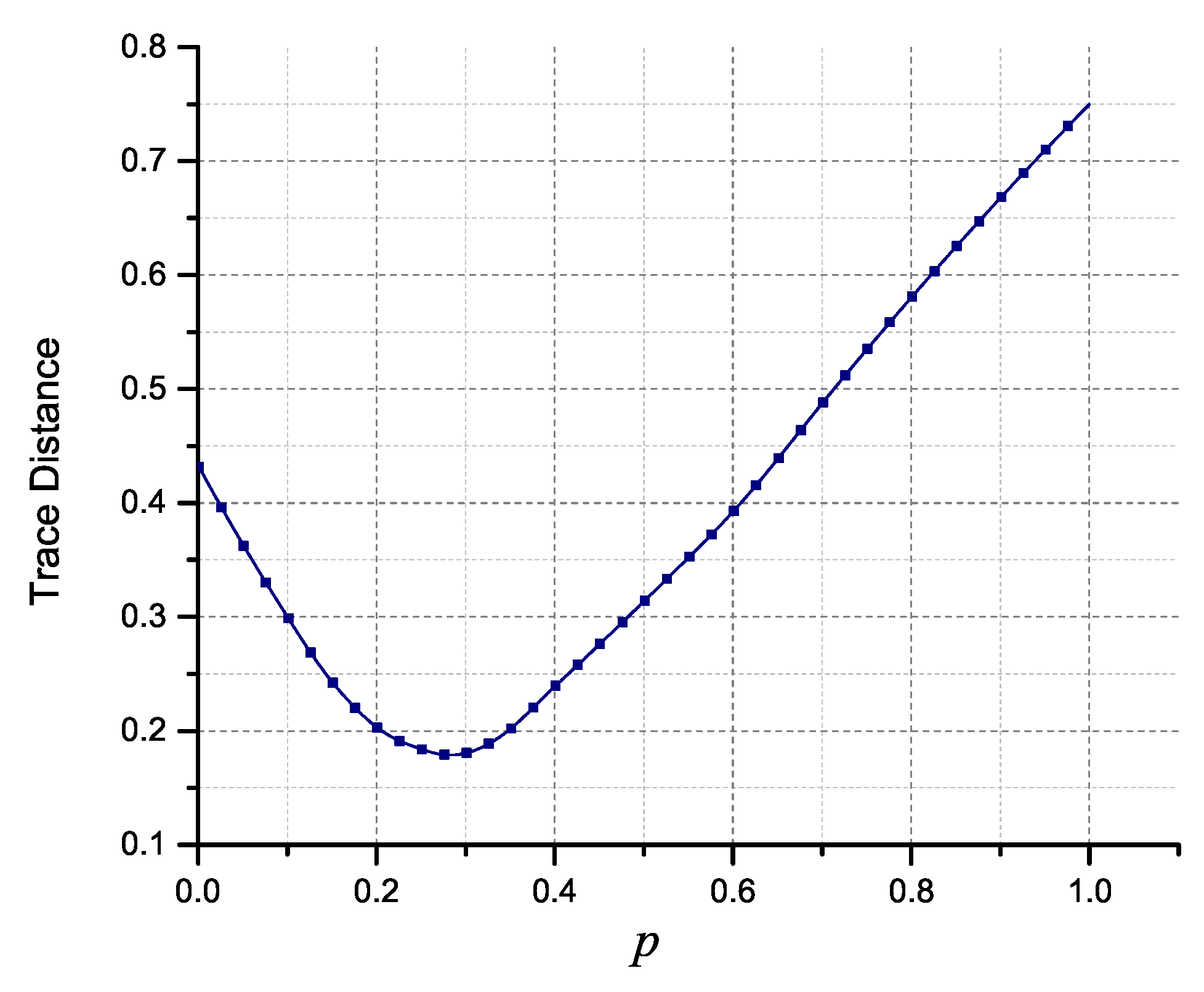
The trace distance between the quantum state ${\rho }_{ABC}$, and the product of the individual quantum states of subsystems A, B, and C is depicted in Figure 7, which is calculated by using Equations (24) and (26) which are derived from the program illustrated in Figure 3. The calculation process should be replaced using the program depicted in Figure 4, in conjunction with Equation (18) and (15), employing optical device systems as carriers.

4. Conclusions and Discussions

We have presented a model capable of obtaining correlations in diagonal quantum states whose density-matrix expressions are unknown. Weak measurements and auxiliary systems are incorporated into this model, and the information required in advance is the dimensions and basis sets of the quantum states involved. An example is provided to illustrate this model. This model can be extended to states involving more particles than those considered in this study, with the number of auxiliary systems increasing as the number of state particles increases.

Unlike conventional correlation verifications, which demand full quantum-state tomography and thus require the collection of extensive raw statistics at the detection side—giving rise to potential side-channel leakage—our protocol extracts the relevant information solely from the pointer displacements. No exchange of raw measurement outcomes among the parties is necessary; all computations are completed locally within Charlie’s four-line weak-coupling device (WCD). Consequently, the scheme substantially mitigates security vulnerabilities originating from detector imperfections.

The proposed circuit can be directly implemented on either linear-optical or NMR platforms. Each additional qubit merely requires one more auxiliary line and a small number of weak measurements, so the overall scaling remains linear. This yields a plug-and-play entanglement-verification module that can be seamlessly integrated into existing BB84, E91, or six-state protocols, functioning as a real-time security-enhancement layer for large-scale quantum networks.

It can also be extended to high-dimensional cases, provided that mutually unbiased bases of the space can be found [46,47], and the more dimensions there are, the more weak measurements and post-selections are required. Therefore, generalizing this model to multipartite systems or high-dimensional circumstances is another challenging issue that requires further consideration. This model can be regarded as a theoretical foundation for experimental implementation, rather than being purely theoretical. We anticipate that this quantum correlation model can be realized using optical devices or NMR systems as carriers.

References

1. Aharonov, Y.; Albert, D.Z.; Vaidman, L. How the Result of a Measurement of a Component of the Spin of a Spin-1/2 Particle Can Turn Out to be 100. Phys. Rev. Lett. 1988, 60, 1351–1354. [Google Scholar] [CrossRef] [PubMed]
2. Dressel, J.; Jordan, A.N. Significance of the imaginary part of the weak value. Phys. Rev. A 2012, 85, 012107. [Google Scholar] [CrossRef]
3. Hariri, A.; Curic, D.; Giner, L.; Lundeen, J.S. Experimental simultaneous readout of the real and imaginary parts of the weak value. Phys. Rev. A 2019, 100, 032119. [Google Scholar] [CrossRef]
4. Luo, W.; Wang, Y.; Liu, J.; Chen, S.; Luo, H. Attosecond resolution in birefringence measurement using real weak value. Opt. Commun. 2025, 586, 131829. [Google Scholar] [CrossRef]
5. Jozsa, R. Complex weak values in quantum measurement. Phys. Rev. A 2007, 76, 044103. [Google Scholar] [CrossRef]
6. Zhang, J.; Guo, X.; Hou, J.; Jie, Z.; Guo, Y. Enhanced Phase Weak Measurement Based on Multiple Weak Interactions. Chin. J. Lasers-Zhongguo Jiguang 2025, 52, 0212003. [Google Scholar] [CrossRef]
7. Araya-Sossa, K.; Orszag, M. Influence of squeezing on the weak-to-strong measurement transition. Phys. Rev. A 2021, 103, 052215. [Google Scholar] [CrossRef]
8. Polonyi, J.; Rachid, I. Elementary Open Quantum States. Symmetry 2021, 13, 1624. [Google Scholar] [CrossRef]
9. Ritchie, N.W.M.; Story, J.G.; Hulet, R.G. Realization of a Measurement of a “Weak Value”. Phys. Rev. Lett. 1991, 66, 1107–1110. [Google Scholar] [CrossRef]
10. Sun, Z.Z.; Pan, D.; Ruan, D.; Long, G.L. One-Sided Measurement-Device-Independent Practical Quantum Secure Direct Communication. J. Light. Technol. 2023, 41, 4680–4690. [Google Scholar] [CrossRef]
11. Dressel, J.; Malik, M.; Miatto, F.M.; Jordan, A.N.; Boyd, R.W. Understanding quantum weak values: Basics and applications. Rev. Mod. Phys. 2014, 86, 307–316. [Google Scholar] [CrossRef]
12. Magaña-Loaiza, O.S.; Mirhosseini, M.; Rodenburg, B.; Boyd, R.W. Amplification of Angular Rotations Using Weak Measurements. Phys. Rev. Lett. 2014, 112, 200401. [Google Scholar] [CrossRef]
13. Higgins, B.L.; Palsson, M.S.; Xiang, G.Y.; Wiseman, H.M.; Pryde, G.J. Using weak values to experimentally determine “negative probabilities” in a two-photon state with Bell correlations. Phys. Rev. A 2015, 91, 012113. [Google Scholar] [CrossRef]
14. Hill, C.; Ralph, J. Weak measurement and control of entanglement generation. Phys. Rev. A 2008, 77, 014305. [Google Scholar] [CrossRef]
15. Das, D.; Arvind. Estimation of quantum states by weak and projective measurements. Phys. Rev. A 2014, 89, 062121. [Google Scholar] [CrossRef]
16. Bernardo, B.D.L.; Azevedo, S.; Rosas, A. Ultrasmall polarization rotation measurements via weak value amplification. Phys. Lett. A 2014, 378, 2029–2033. [Google Scholar] [CrossRef]
17. Pramanik, T.; Majumdar, A.S. Improving the fidelity of teleportation through noisy channels using weak measurement. Phys. Lett. A 2013, 377, 3209–3215. [Google Scholar] [CrossRef]
18. Zhu, X.; Wei, Q.; Liu, Q.; Wu, S.J. Negative probabilities and information gain in weak measurements. Phys. Lett. A 2013, 377, 2505–2509. [Google Scholar] [CrossRef]
19. Ciccarello, F.; Palma, G.M.; Giovannetti, V. Collision-model-based approach to non-Markovian quantum dynamics. Phys. Rev. A 2013, 87, 040103. [Google Scholar] [CrossRef]
20. Allahverdyan, A.; Nieuwenhuizen, T. Extraction of work from a single thermal bath in the quantum regime. Phys. Rev. Lett. 2000, 85, 1799–1802. [Google Scholar] [CrossRef]
21. Lorenzo, S.; Ciccarello, F.; Palma, G.M. Composite quantum collision models. Phys. Rev. A 2017, 96, 032107. [Google Scholar] [CrossRef]
22. Harris, J.; Boyd, R.W.; Lundeen, J.S. Weak Value Amplification Can Outperform Conventional Measurement in the Presence of Detector Saturation. Phys. Rev. Lett. 2017, 118, 070802. [Google Scholar] [CrossRef]
23. Xu, L.; Liu, Z.; Datta, A.; Knee, G.C.; Lundeen, J.S.; Lu, Y.q.; Zhang, L. Approaching Quantum-Limited Metrology with Imperfect Detectors by Using Weak-Value Amplification. Phys. Rev. Lett. 2020, 125, 080501. [Google Scholar] [CrossRef] [PubMed]
24. Chaturvedi, S. Mutually unbiased bases. Pramana-J. Phys. 2002, 59, 345–350. [Google Scholar] [CrossRef]
25. Wootters, W.; Fields, B. Optimal State Determination by Mutually Unbiased Measurements. Ann. Phys. 1989, 191, 363–381. [Google Scholar] [CrossRef]
26. Nielsen, M.A.; Chuang, I.L. Quantum Computation and Quantum Information, 1st ed.; Cambridge University Press: Cambridge, UK, 2000. [Google Scholar]
27. Wang, H.; Wang, J. An Open Quantum System Interacting with an Interference Engineering Environment. Entropy 2025, 27, 228. [Google Scholar] [CrossRef]
28. Abdelmagid, R.; Alshehhi, K.; Sadiek, G. Entanglement Degradation in Two Interacting Qubits Coupled to Dephasing Environments. Entropy 2023, 25, 1458. [Google Scholar] [CrossRef]
29. Ferreri, A.; Domina, M.; Rizzuto, L.; Passante, R. Spontaneous Emission of an Atom Near an Oscillating Mirror. Symmetry 2019, 11, 1384. [Google Scholar] [CrossRef]
30. Park, C.Y.; Cho, J. Correlations in local measurements and entanglement in many-body systems. Phys. Rev. A 2018, 98, 012107. [Google Scholar] [CrossRef]
31. Smirne, A.; Breuer, H.P.; Piilo, J.; Vacchini, B. Initial correlations in open-systems dynamics The Jaynes-Cummings model. Phys. Rev. A 2010, 82, 062114. [Google Scholar] [CrossRef]
32. Uchiyama, C. Exploring initial correlations in a Gibbs state by application of external field. Phys. Rev. A 2012, 85, 052104. [Google Scholar] [CrossRef]
33. Aharonov, Y.; Rohrlich, D. Quantum Paradoxes: Quantum Theory for the Perplexed; WILEY-VCH Verlag GmbH: Weinheim, Germany, 2005. [Google Scholar]
34. Brodutch, A.; Cohen, E. Nonlocal Measurements via Quantum Erasure. Phys. Rev. Lett. 2016, 116, 070404. [Google Scholar] [CrossRef] [PubMed]
35. Rastegin, A.E. Partitioned trace distances. Quantum Inf. Process. 2010, 9, 61–73. [Google Scholar] [CrossRef]
36. Rana, S.; Parashar, P.; Lewenstein, M. Trace-distance measure of coherence. Phys. Rev. A 2016, 93, 012110. [Google Scholar] [CrossRef]
37. Wang, Q. Optimal Trace Distance and Fidelity Estimations for Pure Quantum States. IEEE Trans. Inf. Theory 2024, 70, 8791–8805. [Google Scholar] [CrossRef]
38. Khasseh, R.; Zhang, J.; Heyl, M.; Rajabpour, M.A. Identifying Quantum Many-Body Integrability and Chaos Using Eigenstate Trace Distances. Phys. Rev. Lett. 2023, 131, 216701. [Google Scholar] [CrossRef]
39. Puchala, Z.; Miszczak, J.A. Bound on trace distance based on superfidelity. Phys. Rev. A 2009, 79, 024302. [Google Scholar] [CrossRef]
40. Nakajima, S.; Utsumi, Y. Speed limits of the trace distance for open quantum system. New J. Phys. 2022, 24, 095004. [Google Scholar] [CrossRef]
41. Wu, S. State tomography via weak measurements. Sci. Rep. 2013, 3, 1193. [Google Scholar] [CrossRef]
42. Duck, I.; Stevenson, P.; Sudarshan, E. The Sense in Which a Weak Measurement of a Spin-1/2 Particles Spin Component Yields a Value 100. Phys. Rev. D 1989, 40, 2112–2117. [Google Scholar] [CrossRef]
43. Lundeen, J.S.; Bamber, C. Procedure for Direct Measurement of General Quantum States Using Weak Measurement. Phys. Rev. Lett. 2012, 108, 070402. [Google Scholar] [CrossRef]
44. Wiseman, H.M. Weak values, quantum trajectories, and the cavity-QED experiment on wave-particle correlation. Phys. Rev. A 2002, 65, 032111. [Google Scholar] [CrossRef]
45. Arvidsson-Shukur, D.R.M.; Braasch Jr, W.F.; De Bievre, S.; Dressel, J.; Jordan, A.N.; Langrenez, C.; Lostaglio, M.; Lundeen, J.S.; Halpern, N.Y. Properties and applications of the Kirkwood-Dirac distribution. New J. Phys. 2024, 26, 121201. [Google Scholar] [CrossRef]
46. Durt, T.; Englert, B.G.; Bengtsson, I.; Życzkowski, K. On mutually unbiased bases. Int. J. Quantum Inf. 2010, 8, 535–640. [Google Scholar] [CrossRef]
47. Spengler, C.; Huber, M.; Brierley, S.; Adaktylos, T.; Hiesmayr, B.C. Entanglement detection via mutually unbiased bases. Phys. Rev. A 2012, 86, 022311. [Google Scholar] [CrossRef]
Figure 1. This diagram illustrates the process of weak measurement in a quantum system. The initial state of the system is denoted by ψ i n , and the initial state of the measuring device is represented by ϕ i n Q d , where Q d is the pointer position of the device. The system and the measuring device are coupled through the unitary operation U ^ = e i i A P d , where A is the observable of interest in the system and P d is the conjugate momentum of the pointer position in the measuring device. This interaction is designed to be weak so as not to significantly disturb the system. Post-selection is then applied, resulting in a final state ψ f i n for the system and reducing the final pointer state ϕ i n Q d A w .
Symmetry 17 01233 g001
Figure 2. Local operations executed by Alice and Bob. Strong couplings and measurements are locally executed, conveying the state composed of system A, B, and C to the system composed of C, C N 1 and C N 2 .
Symmetry 17 01233 g002
Figure 3. Local operations executed by Charlie. C N 1 , C N 2 , and C are, respectively, strongly coupled to auxiliary particles C N 1 , C N 2 and C . Four lines of operations are to be continued, comprising three auxiliary lines and the ρ C N 1 C N 2 C line, namely WCD1, WCD2, WCD3, and WCD4.
Symmetry 17 01233 g003
Figure 4. Four lines of WCD. WCD1 abstracts the information of the state ρ C N 1 C N 2 C . WCD2, WCD3, and WCD4 abstract the information of ρ A , ρ B , and ρ C , respectively. Q d j i presents the pointer position of the weak measuring device which is conjugate to the momentum operator P d in the interaction Hamiltonian H int t = g ( t ) A P d .
Symmetry 17 01233 g004
Figure 5. Quantum-circuit symbol for the controlled-NOT (CNOT) gate. The upper line denotes the control qubit, the lower line denotes the target qubit.
Symmetry 17 01233 g005
Figure 6. If ν 0 , a CNOT unitary operation must be applied to the respective subsystems (one of the particles in an auxiliary state) to ensure that the trace distance between the states ρ A B C and ρ A ρ B ρ C remain unchanged.
Symmetry 17 01233 g006
Figure 7. The trace distance between the quantum state ρ A B C and the product of the individual quantum states of subsystems A, B, and C is plotted versus p.
Symmetry 17 01233 g007