An Adaptive Initialization and Reproduction-Based Evolutionary Algorithm for Tackling Bi-Objective Feature Selection in Classification

Abstract

As a commonly used method in classification, feature selection can be treated as a bi-objective optimization problem, whose objectives are to minimize both the classification error and the number of selected features, suitable for multi-objective evolutionary algorithms (MOEAs) to tackle. However, due to the discrete optimization environment and the increasing number of features, traditional MOEAs could face shortcomings in searching abilities, especially for large-scale or high-dimensional datasets. Thereby, in this work, an adaptive initialization and reproduction-based evolutionary algorithm (abbreviated as AIR) is proposed, specifically designed for addressing bi-objective feature selection in classification. In AIR, an adaptive initialization mechanism (abbreviated as AI) and an adaptive reproduction method (abbreviated as AR) have been both designed by analyzing the characteristics of currently selected solutions in order to improve their search abilities and balance the convergence and diversity performances. Moreover, the designing of adaptive initialization also utilizes the implicit symmetry of solutions generated around some interpolation axes in the objective space. In the experiments, AIR is comprehensively compared with five state-of-the-art MOEAs in a list of 20 real-life classification datasets, with its the statistical performance being overall the best in terms of several indicators.

1. Introduction

In the past few decades, evolutionary algorithms (EAs) [1] have been commonly adopted for tackling multi-objective optimization problems (MOPs) [2] with multiple contradictory objectives to pursue, earning the name multi-objective evolutionary algorithms (MOEAs) [3]. To date, large numbers of MOEAs have already been proposed and can be briefly divided into the following categories: the dominance-based framework that uses the nondominated sorting method for environmental selection, such as the most classic dominance-based framework NSGA-II [4], its improved version based on reference points [5], a strengthened dominance-based algorithm for many-objective optimization [6], and one with explicit variable space diversity management [7]; the decomposition-based framework that decomposes an MOP into single-objective problems based on weight vectors, such as the most classic decomposition-based framework MOEA/D [8], its improved version based on differential evolution [9] or stable matching [10], and one based on symbiotic organism search [11]; the indicator-based framework that utilizes specific performance indicators for truncation, such as the most classic indicator-based framework based on the hypervolume indicator [12], one based on boundary protection [13], one based on analyzing dominance move [14], and a bi-indicator-driven indicator-based framework [15]. There are in addition many other excellent MOEA frameworks, such as the surrogate-based framework [16], the classifier-based framework [17], a three-stage MOEA [18], and the multitasking MOEA [19].

With the help of population-based searching abilities and no need for domain knowledge, MOEAs have been widely utilized to solve real-life optimization problems, such as network construction [20], task offloading [21], community detection [22], and the bi-objective feature selection problem [23] that has been specially focused on in this work. More specifically, feature selection [24] is a data preprocessing technique, selecting only a subset of useful features for classification, especially in high-dimensional datasets [25]. Aiming at minimizing the ratio of selected features, i.e., the first objective, and the ratio of classification errors, the second objective, feature selection then becomes a multi-objective optimization problem, formally presented as follows [26].

$$\begin{array}{cc}\hfill & minimize\mathit{F}\left(\mathit{x}\right)={(f_1\left(\mathit{x}\right),f_2\left(\mathit{x}\right),\dots ,f_M\left(\mathit{x}\right))}^T\hfill \\ \hfill & subjectto\mathit{x}=(x_1,x_2,\dots ,x_D),x_i=\{0,1\}\hfill \end{array}$$

(1)

where D represents the full number of features that can be selected in the decision space, and M denotes the number of objectives to be optimized, which is set to two in this work. $\mathit{F}\left(\mathit{x}\right)$ is the objective vector of solution $\mathit{x}$, and $f_i\left(\mathit{x}\right)$ denotes the corresponding objective value in the direction of the ith objective. Moreover, $\mathit{x}=(x_1,x_2,\dots ,x_D)$ represents the decision vector of a certain solution, where $x_i=1$ indicates that the ith feature is selected and $x_i=0$ indicates not being selected.

To be more specific, the first objective function $f_1\left(\mathit{x}\right)$, which denotes the ratio of selected features in this work, is defined as follows:

$$f_1\left(\mathit{x}\right)={\sum }_{i=1}^D{x}_i/D$$

(2)

the value of which discretely ranges from 0 to 1 (i.e., $0,1/D,2/D,\dots ,1$). In addition, given the results of $TP$ (True Positive), $TN$ (True Negative), $FP$ (False Positive), and $FN$ (False Negative), the second objective function $f_2\left(\mathit{x}\right)$, denoting the ratio of classification errors related to the above selected features, can be further defined as follows:

$$f_2\left(\mathit{x}\right)={\displaystyle \frac{FP+FN}{TP+TN+FP+FN}}$$

(3)

However, despite of their various applications in the field of optimization, traditional MOEAs may still face the curse of dimensionality in tackling the bi-objective feature selection problem, when the number of features increases to high dimensionality, causing a lack of search abilities in finding nondominated solutions. Many existing research works have already attempted to solve this issue [27], but many of these either have complicated algorithm frameworks or need to preset a large number of fixed parameters. Furthermore, it is also difficult to balance well algorithm performance between relatively lower-dimensional datasets and higher-dimensional ones, in terms of both diversity and convergence.

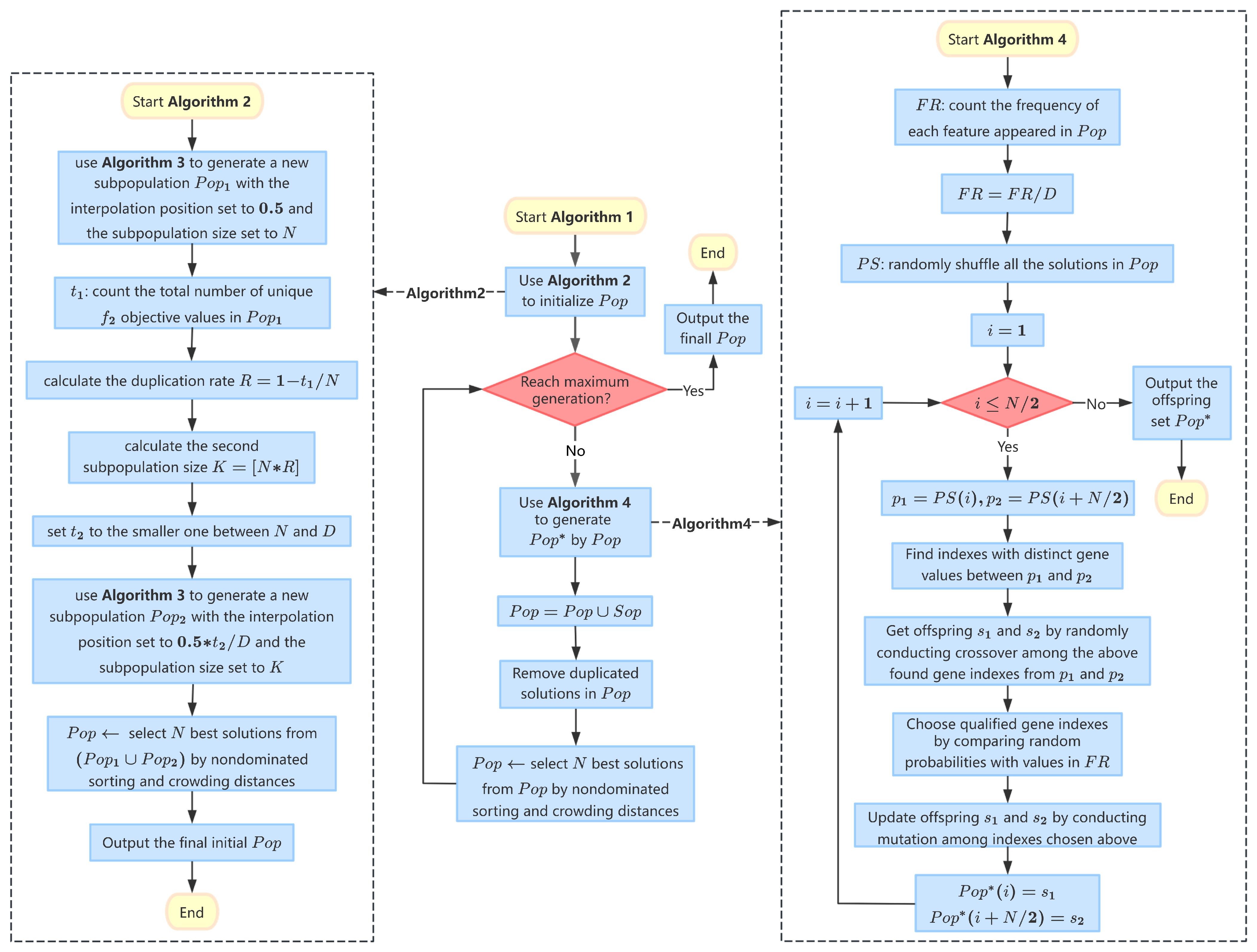
Therefore, in this paper, a simple and effective MOEA framework based on the specially designed adaptive initialization and reproduction mechanisms (abbreviated as AIR) is proposed for addressing the bi-objective feature selection problem in classification datasets. In the proposed AIR algorithm, an adaptive initialization mechanism is designed to provide a promising start for the later evolution and to pursue faster convergence, while an adaptive reproduction method is also adopted to generate more diverse offspring and to avoid potential pre-maturity in convergence. Furthermore, combining the proposed adaptive initialization and reproduction methods together not only increases the search abilities of AIR in finding nondominated solutions, but also helps to maintain a better balance between population diversity and algorithm convergence across the whole evolution. In this way, AIR is then able to deal with more universal optimization environments, across various feature dimensions, from a lower dimensionality to a higher one.

Moreover, it should also be noted that the primary focus of this paper is not on parameter tuning but rather on introducing an innovative adaptive initialization and reproduction strategy for MOEAs in the context of bi-objective feature selection. The key parameters utilized in the adaptive initialization and reproduction processes of AIR are not arbitrarily set but are instead derived from an analysis of the solution distribution in the objective space and the feature frequency within the current population. This adaptive mechanism allows AIR to dynamically balance the exploration and exploitation of the solution space, maintaining a healthy diversity while gradually converging toward promising regions. This is particularly advantageous when dealing with high-dimensional datasets, where the complexity of the feature space and the trade-offs between the two objectives (feature reduction and classification accuracy) are most pronounced. By adaptively adjusting key parameters in response to the evolving characteristics of the population, AIR can effectively navigate the challenges of high-dimensional bi-objective feature selection, which is a significant contribution to the field of MOEAs.

The remainder of this paper is organized as follows. First, related works about multi-objective evolutionary feature selection are discussed in Section 2. Then, the proposed AIR algorithm and its two important components (AI and AR) are illustrated in Section 3. Furthermore, the essential experimental setups are given in Section 4, while all the empirical results are analyzed in Section 5. Finally, the conclusions and future work are both summarized in Section 6.

2. Related Works

The field of multi-objective evolutionary feature selection adopts MOEAs for tackling feature selection problems, which can be roughly categorized into wrapper-based approaches or filter-based ones [28]. In general, wrapper-based methods [29,30] normally adopt certain classification models, such as SVM (Support Vector Machine) or KNN (k-Nearest Neighbor), to evaluate the corresponding classification accuracy as the result of the currently selected feature subsets. Conversely, filter-based methods [31,32] do not rely on any classifier, but directly analyze the explicit or implicit relationship between features and the corresponding classes in the classification datasets, without verifying the classification result for any selected feature subset. Thus, a wrapper based approach is normally more accurate but could consume considerable computational cost due to the real-time classification process during evolution.

Therefore, this paper focuses on studying wrapper-based approaches for evolutionary bi-objective feature selection, attempting to increase the search abilities by improving the initialization and reproduction processes, and to decrease the computational cost by selecting fewer features for classification. Many existing works have already studied similar topics and proposed many inspiring MOEAs specifically for addressing the bi-objective feature selection problem, in recent years.

For instance, in 2020, Xu et al. [33] proposed a segmented initialization method and an offspring modification method, named SIOM; however, its key parameter settings are all fixed and cannot be adaptively altered for different classification datasets, which is not suitable for tackling high-dimensional feature selection. Tian et al. in 2020 [34] proposed a sparse MOEA for tackling bi-objective feature selection, named SparseEA, based on the analyses of each single feature performance before the start of the main evolution; however, the analyses may require a large computational cost as the dimensionality of features increases. Subsequently, Zhang et al. further [35] proposed an improved version of the previous Sparse, named SparseEA2, which has a modified two-layer encoding scheme assisted by variable grouping techniques but still incurs considerable computational cost for solving high-dimensional feature selection problems. In 2021, Xu et al. [36] proposed a duplication analysis-based evolutionary algorithm, which is combined with an efficient reproduction method; however, its performance has not yet been tested in cases of high-dimensional feature selection. In 2022, Cheng et al. [25] proposed a steering matrix-based MOEA specifically for tackling high-dimensional feature selection; however, its performance on relatively lower-dimensional datasets is not validated, which might restrict its universality. Later, inspired by the aforementioned work [36], Jiao et al. in 2024 [37] designed a problem reformulation mechanism to further improve the process of handling solution duplication, named PRDH (which we use as a comparison algorithm in our experiments), whose applicability remains unconfirmed in different MOEA frameworks. In the same year, Xu et al. [38] proposed a bi-search mechanism-based evolutionary algorithm, named BSEA (which we use as a comparison algorithm in our experiments), which was specifically designed to overcome the challenge of search abilities for high-dimensional feature selection problems; however, this relies on a rather complicated multi-task MOEA framework consisting of two dynamic subpopulations. Most recently, Hang et al. [26] designed a probe population-based initialization method to improve the search ability in high-dimensional feature space; however, its iterative exploration of probe populations may incur considerable computational cost. More related works about evolutionary multi-objective feature selection in classification can be found in the most recent survey [27].

Thus, in this work, the design of a simple and effective MOEA framework is attempted, with the aim of improving the initialization and reproduction processes, with adaptively set parameters, to create a more universal algorithm suitable for handling both lower-dimensional classification datasets and higher-dimensional ones.

3. Proposed Methods

In this section, we first introduce the general framework of the proposed AIR algorithm, and then, respectively, illustrate its essential components, the adaptive initialization method (AI) and the adaptive reproduction method (AR).

3.1. General Framework

Algorithm 1 demonstrates the general framework of AIR, which inputs the population size N and the number of total features D as the initial parameters. It can be seen that the general framework of AIR is similar to other dominance-based MOEAs, but adopts the specifically designed methods for initialization and reproduction, i.e., the adaptive initialization method (AI) and the adaptive reproduction method (AR). Moreover, the environmental selection process has also been slightly modified by adding the removal of duplicated solutions in the current union population $Pop$, as can be seen from Line 5 in Algorithm 1. Then, the truncation method uses the nondominated sorting and crowding distances, introduced in NSGA-II [4] to reserve the best N solutions in $Pop$ for the next generation, as shown by Line 6 in Algorithm 1. The termination criterion of AIR is counted by the accumulated number of so-far evaluated objective functions, which is equal to the number of all the solutions generated during evolution. For the experiments carried out for this paper, the termination criterion was set to $100\ast N$, meaning 100 generations of iterative evolution, representing a compromise between convergence and cost. A more intuitive overview of the proposed AIR algorithm is illustrated in Figure 1, with Algorithm 1, Algorithm 2 (invoking Algorithm 3), and Algorithm 4, respectively, specified in procedures. Furthermore, the two essential components of AIR, AI and AR, are, respectively, explained in the following two sections.

Algorithm 1  $AIR(N,D)$

Input: initial population size N, number of full features D; Output: final reserved population $Pop$; 1: $Pop=AI(N,D)$; $//$ Algorithms 2 and 3 2: while not reaching the termination criterion do 3:     $Po{p}^{\ast }=AR(N,D,Pop)$; $//$ Algorithm 4 4:     $Pop=Pop\cup Po{p}^{\ast }$; 5:     $Pop\leftarrow$ remove duplicated decision vectors in $Pop$; 6:    $Pop\leftarrow$ select the best N solutions in $Pop$ by traditional methods of nondominated sorting and crowding distances; 7: end while

3.2. Adaptive Initialization

The proposed adaptive initialization (AI) process of AIR is shown in Algorithm 2, which also invokes the following Algorithm 3. As can be seen from Algorithm 2, we first initialize $Po{p}_1$ as a sample subpopulation located at the middle of the objective space, by means of invoking Algorithm 3. The input parameters of Algorithm 3 contains a key parameter value of 0.5, which acts as the interpolation position $I_t$ where new solutions will be randomly generated around in the objective space. To be more specific, in Line 4 of Algorithm 3, the input interpolation position is compared with a random probability that judges whether to select the current feature. Therefore, the 0.5 interpolation position input value means randomly creating new solutions around $f_1=0.5$, which is roughly located at the middle of the objective space. Then, Lines 2 and 3 in Algorithm 2 calculate the duplication rate which adaptively decides the number of new solutions needed to be initialized and located at the front of the objective space. Basically, the more duplicated $f_2$ objective values existing, the larger $Po{p}_2$ is initialized by Algorithm 3. This time, as shown in Lines 5 and 6 of Algorithm 2, the input interpolation position for $Po{p}_2$ is set to a much smaller value than 0.5, and is closely related with the comparison between N and D, aiming at randomly creating solutions with much smaller sizes of selected feature subsets. At last, a total of N best solutions will be reserved and selected from the combination of the previously initialized $Po{p}_1$ and $Po{p}_2$, via the traditional nondominated sorting and crowding distance methods [4].

Algorithm 2  $AI(N,D)$

Input: initial population size N, number of full features D; Output: initial population $Pop$; 1: $Po{p}_1=GetSubPop(N,D,0.5)$; 2: $t_1\leftarrow$ get the total number of unique $f_2$ objective values in $Po{p}_1$; 3: $R=1-t_1/N$; $//$ calculate the duplication rate 4: $K=[N\ast R]$; $//$ round to the nearest whole 5: $t_2\leftarrow$ get the minimum value between N and D; 6: $Po{p}_2=GetSubPop(K,D,0.5\ast t_2/D)$; 7: $Pop\leftarrow$ select the best N solutions in $(Po{p}_1\cup Po{p}_2)$ via the traditional methods of nondominated sorting and crowding distances;

Algorithm 3  $GetSubPop(K,D,I_t)$

Input: required subpopulation size K, number of full features D, interpolation $I_t$; Output: new subpopulation $SubPop$; 1: $SubPop=Zeros(K,D)$; $//$ create a zero matrix of $K\ast D$ 2: for  $i=1,2,\dots ,K$do 3:     for $j=1,2,\dots ,D$ do 4:         if $\rho <I_t$then$//$ probability $\rho$ is a randomized from 0 to 1 5:             $SubPop(i,j)=1$; $//$ select the jth feature in the decision space for the ith solution in $SubPop$ 6:         end if 7:     end for 8: end for

Figure 2 shows an example of how the proposed adaptive initialization method in AIR works when the population size is set as $N=8$. At first, a subpopulation $Po{p}_1$ with the size of eight solutions is initialized, at the middle of the objective space, located around the interpolation position, i.e., $f_1=0.5$. Here, $Po{p}_1$ acts as a normal subpopulation for sampling, whose solutions will be analyzed in the direction of $f_2$ for calculating the duplication rate R. As shown in Figure 2, $Po{p}_1$ has a total of eight solutions but only four unique $f_2$ values (i.e., $t_1=4$), making $R=1-4/8$ (i.e., $R=0.5$) in this case. Thus, a second subpopulation $Po{p}_2$ with the size of four solutions (i.e., $K=[8\ast 0.5]$) is then initialized and located around the interpolation position of $f_1=N/D\ast 0.5$, with $N=8$ in this case. We assume that N is far smaller than D, which is rather common in high-dimensional cases, thereby making the interpolation position of $Po{p}_2$ distributed at the front of the objective space. Here, $Po{p}_2$ acts as a pioneer subpopulation for exploring more promising regions in the objective space, with relatively much smaller sizes of selected feature subsets. In this way, the hybrid initial population is made up of both the normal and the pioneer subpopulations, with an adaptively set ratio based on analyzing the duplication of solutions in the $f_2$ objective direction. This is quite reasonable because a more sparse feature space normally leads to more duplicated $f_2$ values, especially when the classification samples are also insufficient for those high-dimensional datasets, resulting in more necessity to explore the front regions in the objective space with smaller sizes of selected feature subsets.

Algorithm 4  $AR(N,D,Pop)$

Input: required offspring number N, number of full features D, current population $Pop$; Output: generated offspring set $Po{p}^{\ast }$; 1: $FR\leftarrow$ calculate the frequency of each feature appeared in $Pop$. 2: $FR\leftarrow$ set all zero values in $FR$ to one. 3: $FR=FR/D$; $//$ get the feature mutation rates 4: $PS\leftarrow$ randomly shuffle all the solutions in $Pop$; 5: for  $i=1,2,\dots ,N/2$do 6:     $p_1=s_1=PS\left(i\right)$ and $p_2=s_2=PS(i+N/2)$; $//$ parents $p_1,p_2$ for offspring $s_1,s_2$ 7:      $t_1\leftarrow$ find indexes with different decision variable values between $p_1$ and $p_2$; 8:     $t_2\leftarrow$ get the length of vector $t_1$; 9:     $t_3\leftarrow$ randomly select an integer from 1 to $t_2$; 10:    $t_4\leftarrow$ randomly select $t_3$ unique integers from 1 to $t_2$; 11:    $j=t_1\left(t_4\right)$; $//$ get decision variable indexes for crossover 12:    $s_1\left(j\right)=p_2\left(j\right)$ and $s_2\left(j\right)=p_1\left(j\right)$; $//$ conduct crossover 13:    $\rho \leftarrow$ get a vector of D random probabilities; 14:    $t_5\leftarrow$ find indexes with values in $\rho$ smaller than the same indexed values in $FR$; 15:    $t_6\leftarrow$ get the length of vector $t_5$; 16:    $\rho \leftarrow$ get a vector of $t_6$ random probabilities; 17:    $t_7\leftarrow$ find indexes with values in $\rho$ smaller than $1/t_6$; 18:    $k=t_5\left(t_7\right)$; $//$ get decision variable indexes for mutation 19:     $s_1\left(k\right)=\neg s_1\left(k\right)$; $//$ adaptive mutation within the first parent 20:     $s_2\left(k\right)\leftarrow$ do the same adaptive mutation operation for $s_2$ from Lines 13 to 19; 21:    $Po{p}^{\ast }\left(i\right)=s_1$ and $Po{p}^{\ast }(i+N/2)=s_2$; 22: end for

3.3. Adaptive Reproduction

The proposed adaptive reproduction (AR) process of AIR is shown in Algorithm 4, which cooperates well with the previously introduced adaptive initialization process for more balance between diversity and convergence performance. As can be seen from Algorithm 4, first, a vector of feature mutation rates $FR$ is calculated based on each feature’s appearance frequency in all the solutions of $Pop$. The mutation rate of each feature is later used in the adaptive mutation operation to decide whether to mutate this feature or not. Then, parent solutions are randomly selected from the current population, with equal mating opportunity for each solution. From Lines 7 to 12 in Algorithm 4, the crossover operation is conducted by selecting only the distinct feature values to exchange between the two parents. Then, from Lines 13 to 20 in Algorithm 4, the adaptive mutation operation is conducted by granting more mutating opportunities for features with more appearances in the current population. Finally, the two newly generated offspring with conducted crossover and mutation operations are added into the final offspring set.

Figure 3 provides a brief example of how the adaptive reproduction process in AIR works, when the total feature number is set as $D=9$. Here, all nine features are stored in the decision vector of each solution, with the value 1 meaning select that feature and the value 0 meaning not to select it. It can be seen that the whole reproduction process is made up of the crossover and mutation operations, which are, respectively, shown on the left and right sides of Figure 3. First of all, it should be noted that Figure 3 only demonstrates the corresponding new offspring for the first parent $p_1$, while two bits indexed at the same positions are exchanged for crossover, i.e., swapping from 1 to 0 or from 0 to 1. Then, the resultant offspring is further mutated, with one bit swapping from 0 to 1, thereby finishing reproducing a new offspring. In Figure 3, bits that are qualified for crossover or mutation are painted gray for distinction, while whether to conduct the final crossover or mutation operation will also be chosen (denoted by ✓). In Figure 3, “Chosen ones” means that those identified genes are chosen for the crossover (i.e., Line 12 in Algorithm 4) or mutation operation (i.e., Line 19 in Algorithm 4). Moreover, it should also be noted that those genes are all chosen from the qualified genes by random probabilities. The crossover process in Figure 3 suggests that only distinct feature values are qualified in the crossover operation, which avoids invalid crossover. The mutation process in Figure 3 follows the adaptive mutation principle designed in Lines 13 to 20 of Algorithm 4, expecting that features with more appearances in the current population could have more chances to be mutated during reproduction. However, as can be seen from Figure 3, although the penultimate gene of the new solution has only a $20\%$$FR$ value, it can still be mutated (but certainly with a lower probability), which somewhat assures the fundamental diversity of those less frequently appearing features.

4. Experimental Setups

In this section, the experimental setups are presented, including the comparison algorithms, the classification datasets, and the essential parameter settings.

4.1. Comparison Algorithms

In this paper, a total of five state-of-the-art MOEAs are used as the algorithms to compare to the proposed AIR. They are BSEA [38] (a bi-search evolutionary algorithm), PRDH [37] (an MOEA based on problem reformulation and duplication handling), PMEA [39] (a polar metric-based evolutionary algorithm), MOEA/D (an MOEA based on decomposition) [8], and NSGA-II (an MOEA based on nondominated sorting and crowding distances) [4]. To be more specific, BSEA and PRDH are both the newest MOEAs specifically proposed for addressing the bi-objective feature selection problem in classification, while BSEA is based on the bi-search multi-task mechanism and PRDH is mainly based on the adaptive duplication handling of solutions. PMEA is an indicator-based MOEA using the polar metric, which can balance well both diversity and convergence performance during evolution. NSGA-II and MOEA/D are the two most classic and universal MOEAs, and are, respectively, based on the dominance and decomposition frameworks.

4.2. Classification Datasets

In the experiments, a series of 20 public real-world classification datasets [40] are adopted as the test problems to challenge both optimization and classification performance for each algorithm in tackling bi-objective feature selection. Each classification dataset is introduced in

Table 1. Attributes of the classification datasets used as the test instances.

No.	Dataset	Feature	Sample	Class
1	Sonar	60	208	2
2	Libras	90	360	15
3	HillValley	100	606	2
4	Synthetic	100	200	5
5	MUSK1	166	476	2
6	Arrhythmia	278	452	13
7	LSVT	310	126	2
8	Madelon	500	2600	2
9	ISOLET1	617	1559	26
10	ISOLET2	617	1560	26
11	Yale	1024	165	15
12	PIE10P	2420	210	10
13	Leukemia1	5327	72	3
14	Tumor9	5726	60	9
15	TOX171	5748	171	4
16	ALLAML	7129	72	2
17	Carcinom	9182	174	11
18	Nci9	9712	60	9
19	Brain2	10,367	50	4
20	Prostate	10,509	102	2

, with the numbers of features sorted in ascending order for the convenience of readers. It can be seen from Table 1 that the numbers of features for all the datasets range from 60 to 10,509, covering a wide variety of features, representing both lower dimensionality and higher dimensionality. Furthermore, the numbers of samples are varied from 50 to 2600, and the numbers of classes range from 2 to 26, both suggesting the competitiveness of the experimental test instances.

4.3. Parameter Settings

The essential parameter settings for all the algorithms are consistent with those utilized in the literature, while the other common parameters adopted in the experiments are as follows. First, every algorithm is coded and run in the open-source public MATLAB (2023b) platform PlatEMO (v3.3) [41]. For the sake of fairness, each experiment is independently run 30 times on each dataset by each algorithm. Furthermore, each classification dataset, before training, is randomly divided into separate training and test subsets with a proportion of $70/30$, based on the stratified split process [36]. Then, a KNN ($K=5$) classifier is combined with a 5-fold cross-validation process to somewhat avoid possible feature selection bias [42]. Finally, the population sizes for all the algorithms are set to 100 and their termination criteria (i.e., the accumulated number of objective functions being evaluated during evolution) are all set to 10,000 (i.e., evolving 100 generations).

5. Empirical Results

In this section, the empirical results are comprehensively studied, including the overall optimization and classification performance of all the algorithms, along with their nondominated solution distribution analyses in the objective space.

5.1. Optimization Performances

The hypervolume (HV) [43] metric, with the global reference point set to $(1,1)$, is utilized as the main indicator in this paper to evaluate the optimization performance of each algorithm. Generally speaking, a larger HV value represents a better optimization performance, considering both convergence and diversity.

Table 2. Mean HV performances of all the algorithms on each dataset. Cells marked in gray mean the best performances in the same rows, and those insignificant differences are prefixed by ★.

Dataset	AIR	BSEA	PRDH	PMEA	MOEA/D	NSGA-II
Sonar	8.023 $\times {10}^{-1}$	★ 7.954 $\times {10}^{-1}$	★ 7.931 $\times {10}^{-1}$	7.774 $\times {10}^{-1}$	★ 7.931 $\times {10}^{-1}$	★ 7.894 $\times {10}^{-1}$
	±2.15 $\times {10}^{-2}$	±2.06 $\times {10}^{-2}$	±1.19 $\times {10}^{-2}$	±2.76 $\times {10}^{-2}$	±2.58 $\times {10}^{-2}$	±2.98 $\times {10}^{-2}$
Libras	7.577 $\times {10}^{-1}$	★ 7.565 $\times {10}^{-1}$	★ 7.467 $\times {10}^{-1}$	7.359 $\times {10}^{-1}$	★ 7.496 $\times {10}^{-1}$	7.476 $\times {10}^{-1}$
	±1.76 $\times {10}^{-2}$	±2.06 $\times {10}^{-2}$	±1.74 $\times {10}^{-2}$	±1.94 $\times {10}^{-2}$	±1.88 $\times {10}^{-2}$	±2.06 $\times {10}^{-2}$
HillValley	6.286 $\times {10}^{-1}$	★ 6.252 $\times {10}^{-1}$	6.186 $\times {10}^{-1}$	5.886 $\times {10}^{-1}$	6.205 $\times {10}^{-1}$	5.879 $\times {10}^{-1}$
	±1.18 $\times {10}^{-2}$	±1.16 $\times {10}^{-2}$	±1.16 $\times {10}^{-2}$	±2.02 $\times {10}^{-2}$	±1.30 $\times {10}^{-2}$	±2.34 $\times {10}^{-2}$
Synthetic	4.298 $\times {10}^{-1}$	★ 4.163 $\times {10}^{-1}$	3.942 $\times {10}^{-1}$	3.764 $\times {10}^{-1}$	3.808 $\times {10}^{-1}$	3.931 $\times {10}^{-1}$
	±2.76 $\times {10}^{-2}$	±3.75 $\times {10}^{-2}$	±3.89 $\times {10}^{-2}$	±4.70 $\times {10}^{-2}$	±3.42 $\times {10}^{-2}$	±3.34 $\times {10}^{-2}$
MUSK1	8.969 $\times {10}^{-1}$	★ 8.967 $\times {10}^{-1}$	8.820 $\times {10}^{-1}$	8.203 $\times {10}^{-1}$	8.636 $\times {10}^{-1}$	8.110 $\times {10}^{-1}$
	±1.32 $\times {10}^{-2}$	±1.47 $\times {10}^{-2}$	±1.77 $\times {10}^{-2}$	±2.82 $\times {10}^{-2}$	±1.96 $\times {10}^{-2}$	±2.58 $\times {10}^{-2}$
Arrhythmia	6.982 $\times {10}^{-1}$	6.831 $\times {10}^{-1}$	6.856 $\times {10}^{-1}$	4.734 $\times {10}^{-1}$	6.665 $\times {10}^{-1}$	6.280 $\times {10}^{-1}$
	±1.23 $\times {10}^{-2}$	±1.54 $\times {10}^{-2}$	±1.41 $\times {10}^{-2}$	±3.72 $\times {10}^{-2}$	±2.11 $\times {10}^{-2}$	±2.99 $\times {10}^{-2}$
LSVT	9.219 $\times {10}^{-1}$	★ 9.182 $\times {10}^{-1}$	9.008 $\times {10}^{-1}$	7.825 $\times {10}^{-1}$	8.483 $\times {10}^{-1}$	7.942 $\times {10}^{-1}$
	±2.51 $\times {10}^{-2}$	±2.48 $\times {10}^{-2}$	±3.05 $\times {10}^{-2}$	±2.38 $\times {10}^{-2}$	±2.99 $\times {10}^{-2}$	±2.99 $\times {10}^{-2}$
Madelon	9.083 $\times {10}^{-1}$	9.053 $\times {10}^{-1}$	9.052 $\times {10}^{-1}$	5.322 $\times {10}^{-1}$	6.269 $\times {10}^{-1}$	5.350 $\times {10}^{-1}$
	±4.11 $\times {10}^{-3}$	±4.44 $\times {10}^{-3}$	±5.62 $\times {10}^{-3}$	±1.10 $\times {10}^{-2}$	±2.98 $\times {10}^{-2}$	±2.90 $\times {10}^{-2}$
ISOLET1	8.657 $\times {10}^{-1}$	8.569 $\times {10}^{-1}$	8.557 $\times {10}^{-1}$	6.509 $\times {10}^{-1}$	7.471 $\times {10}^{-1}$	6.645 $\times {10}^{-1}$
	±1.10 $\times {10}^{-2}$	±1.02 $\times {10}^{-2}$	±9.38 $\times {10}^{-3}$	±1.19 $\times {10}^{-2}$	±1.67 $\times {10}^{-2}$	±1.06 $\times {10}^{-2}$
ISOLET2	8.954 $\times {10}^{-1}$	★ 8.934 $\times {10}^{-1}$	8.877 $\times {10}^{-1}$	6.774 $\times {10}^{-1}$	7.787 $\times {10}^{-1}$	6.810 $\times {10}^{-1}$
	±7.18 $\times {10}^{-3}$	±8.52 $\times {10}^{-3}$	±1.04 $\times {10}^{-2}$	±1.09 $\times {10}^{-2}$	±1.00 $\times {10}^{-2}$	±1.64 $\times {10}^{-2}$
Yale	6.957 $\times {10}^{-1}$	★ 6.884 $\times {10}^{-1}$	6.543 $\times {10}^{-1}$	4.898 $\times {10}^{-1}$	5.227 $\times {10}^{-1}$	4.902 $\times {10}^{-1}$
	±3.71 $\times {10}^{-2}$	±3.53 $\times {10}^{-2}$	±4.62 $\times {10}^{-2}$	±2.77 $\times {10}^{-2}$	±2.71 $\times {10}^{-2}$	±2.01 $\times {10}^{-2}$
PIE10P	9.455 $\times {10}^{-1}$	9.289 $\times {10}^{-1}$	9.359 $\times {10}^{-1}$	5.944 $\times {10}^{-1}$	6.418 $\times {10}^{-1}$	5.971 $\times {10}^{-1}$
	±1.67 $\times {10}^{-2}$	±2.15 $\times {10}^{-2}$	±2.02 $\times {10}^{-2}$	±1.00 $\times {10}^{-2}$	±1.51 $\times {10}^{-2}$	±9.42 $\times {10}^{-3}$
Leukemia1	9.571 $\times {10}^{-1}$	★ 9.516 $\times {10}^{-1}$	★ 9.392 $\times {10}^{-1}$	5.240 $\times {10}^{-1}$	5.432 $\times {10}^{-1}$	5.261 $\times {10}^{-1}$
	±3.34 $\times {10}^{-2}$	±3.27 $\times {10}^{-2}$	±4.82 $\times {10}^{-2}$	±2.08 $\times {10}^{-2}$	±2.32 $\times {10}^{-2}$	±2.05 $\times {10}^{-2}$
Tumor9	4.695 $\times {10}^{-1}$	★ 4.678 $\times {10}^{-1}$	★ 4.426 $\times {10}^{-1}$	2.768 $\times {10}^{-1}$	2.781 $\times {10}^{-1}$	2.788 $\times {10}^{-1}$
	±5.74 $\times {10}^{-2}$	±7.92 $\times {10}^{-2}$	±7.55 $\times {10}^{-2}$	±2.32 $\times {10}^{-2}$	±2.75 $\times {10}^{-2}$	±2.82 $\times {10}^{-2}$
TOX171	8.062 $\times {10}^{-1}$	★ 7.955 $\times {10}^{-1}$	7.532 $\times {10}^{-1}$	4.878 $\times {10}^{-1}$	4.880 $\times {10}^{-1}$	4.810 $\times {10}^{-1}$
	±4.02 $\times {10}^{-2}$	±3.29 $\times {10}^{-2}$	±4.08 $\times {10}^{-2}$	±1.39 $\times {10}^{-2}$	±1.69 $\times {10}^{-2}$	±1.34 $\times {10}^{-2}$
ALLAML	9.654 $\times {10}^{-1}$	★ 9.641 $\times {10}^{-1}$	★ 9.627 $\times {10}^{-1}$	5.140 $\times {10}^{-1}$	5.278 $\times {10}^{-1}$	5.144 $\times {10}^{-1}$
	±3.77 $\times {10}^{-2}$	±3.21 $\times {10}^{-2}$	±2.94 $\times {10}^{-2}$	±1.35 $\times {10}^{-2}$	±1.45 $\times {10}^{-2}$	±1.49 $\times {10}^{-2}$
Carcinom	8.801 $\times {10}^{-1}$	8.581 $\times {10}^{-1}$	8.330 $\times {10}^{-1}$	5.174 $\times {10}^{-1}$	5.226 $\times {10}^{-1}$	5.156 $\times {10}^{-1}$
	±2.90 $\times {10}^{-2}$	±2.91 $\times {10}^{-2}$	±4.22 $\times {10}^{-2}$	±9.14 $\times {10}^{-3}$	±1.20 $\times {10}^{-2}$	±9.63 $\times {10}^{-3}$
Nci9	4.831 $\times {10}^{-1}$	★ 4.767 $\times {10}^{-1}$	4.321 $\times {10}^{-1}$	2.449 $\times {10}^{-1}$	2.460 $\times {10}^{-1}$	2.486 $\times {10}^{-1}$
	±5.53 $\times {10}^{-2}$	±7.73 $\times {10}^{-2}$	±5.99 $\times {10}^{-2}$	±2.25 $\times {10}^{-2}$	±3.36 $\times {10}^{-2}$	±2.92 $\times {10}^{-2}$
Brain2	7.474 $\times {10}^{-1}$	★ 7.130 $\times {10}^{-1}$	★ 7.151 $\times {10}^{-1}$	3.858 $\times {10}^{-1}$	3.883 $\times {10}^{-1}$	3.820 $\times {10}^{-1}$
	±6.18 $\times {10}^{-2}$	±6.35 $\times {10}^{-2}$	±7.98 $\times {10}^{-2}$	±2.47 $\times {10}^{-2}$	±2.37 $\times {10}^{-2}$	±2.34 $\times {10}^{-2}$
Prostate	9.500 $\times {10}^{-1}$	★ 9.461 $\times {10}^{-1}$	★ 9.422 $\times {10}^{-1}$	4.606 $\times {10}^{-1}$	4.658 $\times {10}^{-1}$	4.595 $\times {10}^{-1}$
	±2.20 $\times {10}^{-2}$	±2.99 $\times {10}^{-2}$	±3.31 $\times {10}^{-2}$	±1.57 $\times {10}^{-2}$	±2.15 $\times {10}^{-2}$	±1.64 $\times {10}^{-2}$

provides the statistic data for the mean performances in terms of the HV values obtained by each algorithm on the tested datasets, with the best performance on each dataset being marked by the gray base color for distinction. It should be noted that a Wilcoxon Test with a significance level set to $5\%$ is also used to identify performance differences, with those with insignificant performance are prefixed by the symbol ★.

First, it can be seen from Table 2 that in all the tested datasets, the proposed algorithm AIR performs the best of all the algorithms in the comparison, and in most of the test instances, the performance advantage over the other algorithms of AIR is rather significant. Since the HV metric takes both diversity and convergence of the nondominated solutions into consideration, the success of AIR in this metric suggests its superiority in both $f_1$ and $f_2$ objective directions. Moreover, the excellent performances of AIR across various kinds of classification datasets also imply its generality and effectiveness of search abilities in tackling bi-objective feature selection, not only on the relatively lower-dimensional datasets but also on the relatively higher-dimensional ones that are more challenging for traditional MOEAs. The advantages of AIR over those MOEAs that are not specifically proposed for addressing the bi-objective feature selection problem (i.e., PMEA, MOEA/D, and NSGA-II) on the high-dimensional datasets appear to be more obvious because of the sparsity of feasible feature space and the growing difficulty of finding nondominated solutions when the total number of features increases. In general, it is implied that AIR overall achieves the best optimization performances compared with all the other algorithms.

5.2. Classification Performances

In this paper, the minimum classification error (MCE, introduced in [36]) and the number of selected features (NSF, introduced in [36]) are used as supplemental metrics to the previously presented HV metric, which could provide additional analyses for the classification performances obtained by each algorithm. More specifically, MCE is the minimum classification error among all the solutions within a final population, denoting the best classification accuracy obtained, while NSF is the corresponding number of selected features for that MCE value (normally rounded up). Generally speaking, a smaller MCE value represents a better classification performance, while a smaller NSF value normally results in a more efficient classification process with relatively less computational cost.

Table 3. Mean MCE and NSF performance of all the algorithms on each dataset. Cells marked in gray mean the best MCE values in the same rows and those insignificant differences are prefixed by ★.

Dataset	AIR	BSEA	PRDH	PMEA	MOEA/D	NSGA-II
Sonar	1.989 $\times {10}^{-1}$	★ 2.081 $\times {10}^{-1}$	2.118 $\times {10}^{-1}$	2.151 $\times {10}^{-1}$	★ 2.091 $\times {10}^{-1}$	★ 2.086 $\times {10}^{-1}$
	NSF ≈ 7	NSF ≈ 5	NSF ≈ 4	NSF ≈ 7	NSF ≈ 6	NSF ≈ 7
Libras	2.413 $\times {10}^{-1}$	★ 2.429 $\times {10}^{-1}$	2.549 $\times {10}^{-1}$	★ 2.467 $\times {10}^{-1}$	★ 2.495 $\times {10}^{-1}$	★ 2.387 $\times {10}^{-1}$
	NSF ≈ 8	NSF ≈ 8	NSF ≈ 7	NSF ≈ 10	NSF ≈ 9	NSF ≈ 10
HillValley	4.011 $\times {10}^{-1}$	★ 4.049 $\times {10}^{-1}$	4.126 $\times {10}^{-1}$	4.185 $\times {10}^{-1}$	4.104 $\times {10}^{-1}$	4.233 $\times {10}^{-1}$
	NSF ≈ 4	NSF ≈ 5	NSF ≈ 3	NSF ≈ 10	NSF ≈ 3	NSF ≈ 9
Synthetic	6.172 $\times {10}^{-1}$	★ 6.333 $\times {10}^{-1}$	6.594 $\times {10}^{-1}$	6.578 $\times {10}^{-1}$	6.672 $\times {10}^{-1}$	★ 6.367 $\times {10}^{-1}$
	NSF ≈ 9	NSF ≈ 7	NSF ≈ 5	NSF ≈ 14	NSF ≈ 12	NSF ≈ 14
MUSK1	9.837 $\times {10}^{-2}$	★ 1.016 $\times {10}^{-1}$	1.196 $\times {10}^{-1}$	★ 9.790 $\times {10}^{-2}$	1.210 $\times {10}^{-1}$	★ 1.091 $\times {10}^{-1}$
	NSF ≈ 21	NSF ≈ 18	NSF ≈ 12	NSF ≈ 30	NSF ≈ 17	NSF ≈ 28
Arrhythmia	3.283 $\times {10}^{-1}$	3.453 $\times {10}^{-1}$	3.424 $\times {10}^{-1}$	4.602 $\times {10}^{-1}$	3.520 $\times {10}^{-1}$	3.856 $\times {10}^{-1}$
	NSF ≈ 8	NSF ≈ 6	NSF ≈ 6	NSF ≈ 58	NSF ≈ 12	NSF ≈ 15
LSVT	8.158 $\times {10}^{-2}$	★ 8.596 $\times {10}^{-2}$	1.053 $\times {10}^{-1}$	★ 9.298 $\times {10}^{-2}$	9.912 $\times {10}^{-2}$	9.825 $\times {10}^{-2}$
	NSF ≈ 7	NSF ≈ 5	NSF ≈ 4	NSF ≈ 53	NSF ≈ 27	NSF ≈ 48
Madelon	9.744 $\times {10}^{-2}$	1.007 $\times {10}^{-1}$	1.009 $\times {10}^{-1}$	3.406 $\times {10}^{-1}$	3.103 $\times {10}^{-1}$	3.413 $\times {10}^{-1}$
	NSF ≈ 7	NSF ≈ 6	NSF ≈ 6	NSF ≈ 137	NSF ≈ 78	NSF ≈ 136
ISOLET1	1.333 $\times {10}^{-1}$	1.491 $\times {10}^{-1}$	1.489 $\times {10}^{-1}$	★ 1.372 $\times {10}^{-1}$	1.495 $\times {10}^{-1}$	★ 1.363 $\times {10}^{-1}$
	NSF ≈ 47	NSF ≈ 34	NSF ≈ 46	NSF ≈ 188	NSF ≈ 107	NSF ≈ 184
ISOLET2	9.544 $\times {10}^{-2}$	1.083 $\times {10}^{-1}$	1.123 $\times {10}^{-1}$	★ 9.551 $\times {10}^{-2}$	1.083 $\times {10}^{-1}$	★ 9.886 $\times {10}^{-2}$
	NSF ≈ 53	NSF ≈ 40	NSF ≈ 57	NSF ≈ 196	NSF ≈ 112	NSF ≈ 193
Yale	3.326 $\times {10}^{-1}$	★ 3.407 $\times {10}^{-1}$	3.785 $\times {10}^{-1}$	★ 3.467 $\times {10}^{-1}$	3.504 $\times {10}^{-1}$	★ 3.474 $\times {10}^{-1}$
	NSF ≈ 14	NSF ≈ 12	NSF ≈ 8	NSF ≈ 324	NSF ≈ 268	NSF ≈ 333
PIE10P	5.889 $\times {10}^{-2}$	7.722 $\times {10}^{-2}$	6.944 $\times {10}^{-2}$	1.017 $\times {10}^{-1}$	1.039 $\times {10}^{-1}$	1.006 $\times {10}^{-1}$
	NSF ≈ 13	NSF ≈ 10	NSF ≈ 11	NSF ≈ 934	NSF ≈ 776	NSF ≈ 923
Leukemia1	4.697 $\times {10}^{-2}$	★ 5.303 $\times {10}^{-2}$	★ 6.667 $\times {10}^{-2}$	1.652 $\times {10}^{-1}$	1.788 $\times {10}^{-1}$	1.667 $\times {10}^{-1}$
	NSF ≈ 3	NSF ≈ 3	NSF ≈ 3	NSF ≈ 2264	NSF ≈ 2060	NSF ≈ 2228
Tumor9	5.833 $\times {10}^{-1}$	★ 5.852 $\times {10}^{-1}$	★ 6.130 $\times {10}^{-1}$	★ 6.000 $\times {10}^{-1}$	★ 6.148 $\times {10}^{-1}$	★ 5.981 $\times {10}^{-1}$
	NSF ≈ 7	NSF ≈ 8	NSF ≈ 5	NSF ≈ 2463	NSF ≈ 2327	NSF ≈ 2460
TOX171	2.126 $\times {10}^{-1}$	★ 2.245 $\times {10}^{-1}$	2.711 $\times {10}^{-1}$	★ 2.170 $\times {10}^{-1}$	2.390 $\times {10}^{-1}$	★ 2.289 $\times {10}^{-1}$
	NSF ≈ 17	NSF ≈ 14	NSF ≈ 13	NSF ≈ 2515	NSF ≈ 2382	NSF ≈ 2501
ALLAML	3.788 $\times {10}^{-2}$	★ 3.939 $\times {10}^{-2}$	★ 4.091 $\times {10}^{-2}$	1.667 $\times {10}^{-1}$	1.727 $\times {10}^{-1}$	1.682 $\times {10}^{-1}$
	NSF ≈ 2	NSF ≈ 2	NSF ≈ 2	NSF ≈ 3098	NSF ≈ 2932	NSF ≈ 3082
Carcinom	1.314 $\times {10}^{-1}$	1.558 $\times {10}^{-1}$	1.833 $\times {10}^{-1}$	★ 1.429 $\times {10}^{-1}$	1.494 $\times {10}^{-1}$	1.481 $\times {10}^{-1}$
	NSF ≈ 19	NSF ≈ 19	NSF ≈ 17	NSF ≈ 4113	NSF ≈ 3993	NSF ≈ 4101
Nci9	5.684 $\times {10}^{-1}$	★ 5.754 $\times {10}^{-1}$	6.246 $\times {10}^{-1}$	6.491 $\times {10}^{-1}$	6.614 $\times {10}^{-1}$	6.439 $\times {10}^{-1}$
	NSF ≈ 8	NSF ≈ 9	NSF ≈ 6	NSF ≈ 4298	NSF ≈ 4093	NSF ≈ 4280
Brain2	2.778 $\times {10}^{-1}$	★ 3.156 $\times {10}^{-1}$	★ 3.133 $\times {10}^{-1}$	3.867 $\times {10}^{-1}$	3.911 $\times {10}^{-1}$	3.933 $\times {10}^{-1}$
	NSF ≈ 4	NSF ≈ 3	NSF ≈ 3	NSF ≈ 4620	NSF ≈ 4533	NSF ≈ 4626
Prostate	5.484 $\times {10}^{-2}$	★ 5.914 $\times {10}^{-2}$	★ 6.344 $\times {10}^{-2}$	2.452 $\times {10}^{-1}$	2.495 $\times {10}^{-1}$	2.495 $\times {10}^{-1}$
	NSF ≈ 5	NSF ≈ 3	NSF ≈ 4	NSF ≈ 4729	NSF ≈ 4598	NSF ≈ 4690

provides the statistical data for the mean performances in terms of the MCE values and the corresponding NSF values (shown below MCE in each row) obtained by each algorithm on the tested datasets, with the best MCE performance on each dataset being marked by the gray base color for distinction. It should be noted that a Wilcoxon Test with a significance level set to $5\%$ is also used to identify the MCE performance differences, with those with insignificant differences being prefixed by the symbol ★.

It can be seen from Table 3 that AIR generally performs the best in terms of the mean MCE metric values on most of the tested datasets (18 out of 20). The only two losses appear on the Libras and MUSK1 datasets, while AIR actually has insignificant performance differences from the corresponding best-performing algorithms (NSGA-II and PMEA). Moreover, AIR achieves much better NSF mean values than NSGA-II and PMEA on these two datasets, implying its better classification efficiency with much smaller sizes of selected feature subsets for classification. On the relatively higher-dimensional datasets, compared with PMEA, MOEA/D, and NSGA-II, the advantages of AIR in terms of the MCE and NSF metrics turn out to be more obvious. For example, on the Prostate dataset, which has the highest dimensionality of features, AIR, BSEA, and PRDH, all show tremendous advantages in terms of reducing the NSF mean values compared to the other three traditional MOEAs (PMEA, MOEA/D, and NSGA-II). AIR, BSEA, and PRDH are all specifically proposed for addressing the bi-objective feature selection problem, however, AIR still performs generally better than BSEA and PRDH, with smaller MCE values and equivalent NSF values. In general, the MCE value denotes the best classification accuracy obtained, while the NSF value normally affects the classification efficiency in computational cost. Therefore, it is suggested that AIR generally achieves the best classification performance compared with all the other algorithms.

5.3. Distribution Analyses

For more intuitive observations of algorithm performance, Figure 4 illustrates the distributions of the final nondominated solutions obtained by each algorithm on the test data, related to the median HV performance over 30 runs. It can be seen from Figure 4 that the proposed algorithm AIR generally performs the best or at least shows competitive performance in terms of both diversity and convergence. For example, in Figure 4a, AIR obtains as good of a $f_1$ value as BSEA and the best $f_2$ value of all the algorithms; in Figure 4b, AIR obtains both the best $f_1$ and best $f_2$ values, better than all the others. In the rest of the cases, AIR performs the best in terms of either the $f_1$ or the $f_2$ objective direction, while finding the most or at least promising numbers of nondominated solutions.

5.4. Computational Time

The efficiency of each algorithm is tested by recording its mean runtime on each dataset, as shown in

Table 4. Mean computational cost in seconds of all the algorithms on each dataset. Cells marked in gray mean the best performances in the same rows and the insignificant differences are prefixed by ★.

Dataset	AIR	BSEA	PRDH	PMEA	MOEA/D	NSGA-II
Sonar	3.011 $\times {10}^1$	2.688 $\times {10}^1$	2.714 $\times {10}^1$	2.802 $\times {10}^1$	2.927 $\times {10}^1$	2.984 $\times {10}^1$
	±2.94 $\times {10}^{-1}$	±1.68 $\times {10}^{-1}$	±2.20 $\times {10}^{-1}$	±3.27 $\times {10}^{-1}$	±4.01 $\times {10}^{-1}$	±4.69 $\times {10}^{-1}$
Libras	5.686 $\times {10}^1$	5.323 $\times {10}^1$	5.425 $\times {10}^1$	5.890 $\times {10}^1$	5.652 $\times {10}^1$	5.822 $\times {10}^1$
	±6.15 $\times {10}^{-1}$	±4.61 $\times {10}^{-1}$	±4.76 $\times {10}^{-1}$	±8.49 $\times {10}^{-1}$	±4.02 $\times {10}^{-1}$	±1.49 $\times {10}^0$
HillValley	1.248 $\times {10}^2$	1.119 $\times {10}^2$	1.128 $\times {10}^2$	1.340 $\times {10}^2$	1.151 $\times {10}^2$	1.326 $\times {10}^2$
	±2.13 $\times {10}^0$	±2.33 $\times {10}^0$	±1.18 $\times {10}^0$	±3.05 $\times {10}^0$	±1.61 $\times {10}^0$	±6.67 $\times {10}^0$
Synthetic	2.921 $\times {10}^1$	2.785 $\times {10}^1$	2.861 $\times {10}^1$	3.012 $\times {10}^1$	3.101 $\times {10}^1$	2.981 $\times {10}^1$
	±3.64 $\times {10}^{-1}$	±5.50 $\times {10}^{-1}$	±2.59 $\times {10}^{-1}$	±3.99 $\times {10}^{-1}$	±4.67 $\times {10}^{-1}$	±6.57 $\times {10}^{-1}$
MUSK1	1.034 $\times {10}^2$	9.229 $\times {10}^1$	9.066 $\times {10}^1$	1.258 $\times {10}^2$	★ 1.032 $\times {10}^2$	1.208 $\times {10}^2$
	±2.70 $\times {10}^0$	±3.01 $\times {10}^0$	±2.32 $\times {10}^0$	±2.75 $\times {10}^0$	±2.18 $\times {10}^0$	±4.83 $\times {10}^0$
Arrhythmia	9.936 $\times {10}^1$	★ 9.912 $\times {10}^1$	★ 1.021 $\times {10}^2$	1.285 $\times {10}^2$	1.045 $\times {10}^2$	1.066 $\times {10}^2$
	±1.41 $\times {10}^0$	±4.56 $\times {10}^0$	±4.98 $\times {10}^0$	±6.52 $\times {10}^0$	±7.06 $\times {10}^0$	±9.50 $\times {10}^0$
LSVT	1.988 $\times {10}^1$	1.895 $\times {10}^1$	1.958 $\times {10}^1$	2.697 $\times {10}^1$	2.594 $\times {10}^1$	2.620 $\times {10}^1$
	±3.40 $\times {10}^{-1}$	±2.11 $\times {10}^{-1}$	±3.93 $\times {10}^{-1}$	±4.42 $\times {10}^{-1}$	±5.66 $\times {10}^{-1}$	±5.62 $\times {10}^{-1}$
Madelon	4.838 $\times {10}^3$	5.059 $\times {10}^3$	5.299 $\times {10}^3$	9.709 $\times {10}^3$	8.107 $\times {10}^3$	9.454 $\times {10}^3$
	±9.79 $\times {10}^1$	±1.99 $\times {10}^2$	±3.21 $\times {10}^2$	±2.29 $\times {10}^2$	±3.63 $\times {10}^2$	±4.08 $\times {10}^2$
ISOLET1	2.404 $\times {10}^3$	★ 2.375 $\times {10}^3$	2.540 $\times {10}^3$	4.430 $\times {10}^3$	3.533 $\times {10}^3$	4.284 $\times {10}^3$
	±9.82 $\times {10}^1$	±1.01 $\times {10}^2$	±1.87 $\times {10}^2$	±1.15 $\times {10}^2$	±1.48 $\times {10}^2$	±1.30 $\times {10}^2$
ISOLET2	2.484 $\times {10}^3$	2.352 $\times {10}^3$	★ 2.492 $\times {10}^3$	4.465 $\times {10}^3$	3.550 $\times {10}^3$	4.351 $\times {10}^3$
	±7.20 $\times {10}^1$	±1.18 $\times {10}^2$	±2.36 $\times {10}^2$	±9.27 $\times {10}^1$	±1.26 $\times {10}^2$	±1.55 $\times {10}^2$
Yale	1.117 $\times {10}^2$	1.036 $\times {10}^2$	1.070 $\times {10}^2$	2.121 $\times {10}^2$	1.829 $\times {10}^2$	2.177 $\times {10}^2$
	±1.81 $\times {10}^0$	±2.23 $\times {10}^0$	±1.61 $\times {10}^0$	±4.37 $\times {10}^0$	±3.41 $\times {10}^0$	±7.76 $\times {10}^0$
PIE10P	6.126 $\times {10}^2$	★ 6.074 $\times {10}^2$	6.621 $\times {10}^2$	1.049 $\times {10}^3$	1.009 $\times {10}^3$	1.052 $\times {10}^3$
	±1.51 $\times {10}^1$	±2.52 $\times {10}^1$	±4.84 $\times {10}^1$	±2.75 $\times {10}^1$	±3.28 $\times {10}^1$	±3.77 $\times {10}^1$
Leukemia1	4.371 $\times {10}^2$	4.502 $\times {10}^2$	5.190 $\times {10}^2$	7.654 $\times {10}^2$	7.216 $\times {10}^2$	7.700 $\times {10}^2$
	±1.18 $\times {10}^1$	±2.17 $\times {10}^1$	±5.44 $\times {10}^1$	±1.86 $\times {10}^1$	±1.47 $\times {10}^1$	±2.28 $\times {10}^1$
Tumor9	3.963 $\times {10}^2$	3.802 $\times {10}^2$	4.267 $\times {10}^2$	6.936 $\times {10}^2$	6.520 $\times {10}^2$	6.970 $\times {10}^2$
	±1.34 $\times {10}^1$	±2.29 $\times {10}^1$	±4.03 $\times {10}^1$	±1.63 $\times {10}^1$	±1.61 $\times {10}^1$	±2.03 $\times {10}^1$
TOX171	1.229 $\times {10}^3$	1.268 $\times {10}^3$	1.416 $\times {10}^3$	2.266 $\times {10}^3$	2.213 $\times {10}^3$	2.301 $\times {10}^3$
	±3.92 $\times {10}^1$	±6.41 $\times {10}^1$	±1.73 $\times {10}^2$	±7.30 $\times {10}^1$	±7.02 $\times {10}^1$	±9.71 $\times {10}^1$
ALLAML	6.357 $\times {10}^2$	6.637 $\times {10}^2$	7.303 $\times {10}^2$	1.072 $\times {10}^3$	1.044 $\times {10}^3$	1.087 $\times {10}^3$
	±2.03 $\times {10}^1$	±3.96 $\times {10}^1$	±7.67 $\times {10}^1$	±3.64 $\times {10}^1$	±3.20 $\times {10}^1$	±2.94 $\times {10}^1$
Carcinom	2.099 $\times {10}^3$	2.222 $\times {10}^3$	2.418 $\times {10}^3$	3.841 $\times {10}^3$	3.803 $\times {10}^3$	3.886 $\times {10}^3$
	±7.28 $\times {10}^1$	±1.35 $\times {10}^2$	±2.68 $\times {10}^2$	±1.15 $\times {10}^2$	±1.32 $\times {10}^2$	±1.54 $\times {10}^2$
Nci9	7.552 $\times {10}^2$	7.941 $\times {10}^2$	8.475 $\times {10}^2$	1.346 $\times {10}^3$	1.251 $\times {10}^3$	1.354 $\times {10}^3$
	±3.00 $\times {10}^1$	±4.13 $\times {10}^1$	±8.18 $\times {10}^1$	±3.42 $\times {10}^1$	±3.33 $\times {10}^1$	±4.12 $\times {10}^1$
Brain2	6.915 $\times {10}^2$	7.246 $\times {10}^2$	7.907 $\times {10}^2$	1.211 $\times {10}^3$	1.114 $\times {10}^3$	1.241 $\times {10}^3$
	±1.99 $\times {10}^1$	±3.49 $\times {10}^1$	±7.64 $\times {10}^1$	±5.41 $\times {10}^1$	±3.20 $\times {10}^1$	±5.73 $\times {10}^1$
Prostate	1.411 $\times {10}^3$	1.481 $\times {10}^3$	1.618 $\times {10}^3$	2.580 $\times {10}^3$	2.482 $\times {10}^3$	2.589 $\times {10}^3$
	±5.38 $\times {10}^1$	±8.34 $\times {10}^1$	±1.71 $\times {10}^2$	±8.19 $\times {10}^1$	±7.54 $\times {10}^1$	±9.32 $\times {10}^1$
Friedman’s Rank	2.262	1.575	2.552	5.305	4.113	5.193

, while a Friedman’s test is also conduct to present the mean ranks (the smaller the better) of all the comparison algorithms on all the datasets. Table 4 indicates that the proposed AIR algorithm generally shows promising efficiency on all the datasets, taking the first place on 8 out of 20 datasets, and achieving the top two rankings on 13 out of 20 datasets. The rank results of Friedman’s test shown in the last row of Table 4 also show that AIR generally ranks the second among all the algorithms, only slightly behind BSEA. Thus, the efficiency of AIR is rather promising, considering that BSEA and PRDH are both fast and competitive state-of-the-art algorithms specifically designed for tackling bi-objective feature selection. This is because both BSEA and PRDH take advantage of their modified initialization methods to pursue the early convergence of initial populations, which makes their sizes of selected feature subsets even smaller than those of AIR, thereby costing less classification time than AIR. Conversely, AIR does not excessively pursue the premature convergence of initial populations, but rather seeks a balance between the diversity and convergence in its adaptive initialization process, which makes AIR less likely to fall into local optima or early maturity than BSEA and PRDH.

5.5. More Comparisons

To further validate the effectiveness of the proposed adaptive initialization strategy, a variant version AIR-Base was designed by replacing the initialization process of AIR with the traditional initialization method used in NSGA-II.

Table 5. Comparison of Mean HV, MCE, and NSF performance between AIR and its variant version AIR-Base. Cells marked in gray mean the best performances and the insignificant differences are prefixed by ★.

Dataset	HV		MCE		NSF
	AIR	AIR-Base	AIR	AIR-Base	AIR	AIR-Base
Sonar	8.023 $\times {10}^{-1}$	★ 7.994 $\times {10}^{-1}$	1.989 $\times {10}^{-1}$	★ 2.027 $\times {10}^{-1}$	6.667 $\times {10}^0$	★ 5.033 $\times {10}^0$
	±2.15 $\times {10}^{-2}$	±2.43 $\times {10}^{-2}$	±2.59 $\times {10}^{-2}$	±3.10 $\times {10}^{-2}$	±3.55 $\times {10}^0$	±3.96 $\times {10}^0$
Libras	7.577 $\times {10}^{-1}$	★ 7.623 $\times {10}^{-1}$	2.413 $\times {10}^{-1}$	★ 2.356 $\times {10}^{-1}$	8.300 $\times {10}^0$	★ 1.017 $\times {10}^1$
	±1.76 $\times {10}^{-2}$	±1.68 $\times {10}^{-2}$	±2.04 $\times {10}^{-2}$	±1.95 $\times {10}^{-2}$	±3.00 $\times {10}^0$	±3.53 $\times {10}^0$
HillValley	6.286 $\times {10}^{-1}$	★ 6.263 $\times {10}^{-1}$	4.011 $\times {10}^{-1}$	★ 4.038 $\times {10}^{-1}$	4.300 $\times {10}^0$	★ 4.033 $\times {10}^0$
	±1.18 $\times {10}^{-2}$	±1.21 $\times {10}^{-2}$	±1.35 $\times {10}^{-2}$	±1.37 $\times {10}^{-2}$	±3.12 $\times {10}^0$	±2.77 $\times {10}^0$
Synthetic	4.298 $\times {10}^{-1}$	★ 4.240 $\times {10}^{-1}$	6.172 $\times {10}^{-1}$	★ 6.233 $\times {10}^{-1}$	9.033 $\times {10}^0$	★ 8.667 $\times {10}^0$
	±2.76 $\times {10}^{-2}$	±3.58 $\times {10}^{-2}$	±3.32 $\times {10}^{-2}$	±4.32 $\times {10}^{-2}$	±4.82 $\times {10}^0$	±4.48 $\times {10}^0$
MUSK1	8.969 $\times {10}^{-1}$	★ 8.970 $\times {10}^{-1}$	9.837 $\times {10}^{-2}$	★ 9.207 $\times {10}^{-2}$	2.100 $\times {10}^1$	★ 2.417 $\times {10}^1$
	±1.32 $\times {10}^{-2}$	±1.66 $\times {10}^{-2}$	±1.58 $\times {10}^{-2}$	±2.06 $\times {10}^{-2}$	±7.48 $\times {10}^0$	±1.11 $\times {10}^1$
Arrhythmia	6.982 $\times {10}^{-1}$	6.858 $\times {10}^{-1}$	3.283 $\times {10}^{-1}$	3.422 $\times {10}^{-1}$	7.900 $\times {10}^0$	8.000 $\times {10}^0$
	±1.23 $\times {10}^{-2}$	±1.70 $\times {10}^{-2}$	±1.38 $\times {10}^{-2}$	±1.91 $\times {10}^{-2}$	±2.35 $\times {10}^0$	±3.90 $\times {10}^0$
LSVT	9.219 $\times {10}^{-1}$	★ 9.251 $\times {10}^{-1}$	8.158 $\times {10}^{-2}$	★ 6.754 $\times {10}^{-2}$	7.100 $\times {10}^0$	★ 1.050 $\times {10}^1$
	±2.51 $\times {10}^{-2}$	±1.90 $\times {10}^{-2}$	±2.79 $\times {10}^{-2}$	±2.04 $\times {10}^{-2}$	±4.12 $\times {10}^0$	±5.02 $\times {10}^0$
Madelon	9.083 $\times {10}^{-1}$	8.436 $\times {10}^{-1}$	9.744 $\times {10}^{-2}$	1.442 $\times {10}^{-1}$	7.033 $\times {10}^0$	2.020 $\times {10}^1$
	±4.11 $\times {10}^{-3}$	±2.18 $\times {10}^{-2}$	±4.58 $\times {10}^{-3}$	±1.96 $\times {10}^{-2}$	±1.45 $\times {10}^0$	±4.59 $\times {10}^0$
ISOLET1	8.657 $\times {10}^{-1}$	7.993 $\times {10}^{-1}$	1.333 $\times {10}^{-1}$	1.185 $\times {10}^{-1}$	4.737 $\times {10}^1$	1.072 $\times {10}^2$
	±1.10 $\times {10}^{-2}$	±9.89 $\times {10}^{-3}$	±1.26 $\times {10}^{-2}$	±6.87 $\times {10}^{-3}$	±1.28 $\times {10}^1$	±2.30 $\times {10}^1$
ISOLET2	8.954 $\times {10}^{-1}$	8.229 $\times {10}^{-1}$	9.544 $\times {10}^{-2}$	7.934 $\times {10}^{-2}$	5.337 $\times {10}^1$	1.121 $\times {10}^2$
	±7.18 $\times {10}^{-3}$	±9.02 $\times {10}^{-3}$	±7.26 $\times {10}^{-3}$	±6.89 $\times {10}^{-3}$	±1.70 $\times {10}^1$	±2.20 $\times {10}^1$
Yale	6.957 $\times {10}^{-1}$	6.370 $\times {10}^{-1}$	3.326 $\times {10}^{-1}$	3.030 $\times {10}^{-1}$	1.353 $\times {10}^1$	1.513 $\times {10}^2$
	±3.71 $\times {10}^{-2}$	±2.99 $\times {10}^{-2}$	±4.11 $\times {10}^{-2}$	±3.62 $\times {10}^{-2}$	±6.22 $\times {10}^0$	±2.13 $\times {10}^1$
PIE10P	9.455 $\times {10}^{-1}$	7.349 $\times {10}^{-1}$	5.889 $\times {10}^{-2}$	8.056 $\times {10}^{-2}$	1.280 $\times {10}^1$	5.637 $\times {10}^2$
	±1.67 $\times {10}^{-2}$	±1.56 $\times {10}^{-2}$	±1.84 $\times {10}^{-2}$	±1.76 $\times {10}^{-2}$	±3.28 $\times {10}^0$	±2.64 $\times {10}^1$
Leukemia1	9.571 $\times {10}^{-1}$	6.261 $\times {10}^{-1}$	4.697 $\times {10}^{-2}$	1.576 $\times {10}^{-1}$	2.933 $\times {10}^0$	1.590 $\times {10}^3$
	±3.34 $\times {10}^{-2}$	±2.38 $\times {10}^{-2}$	±3.68 $\times {10}^{-2}$	±3.91 $\times {10}^{-2}$	±1.31 $\times {10}^0$	±7.08 $\times {10}^1$
Tumor9	4.695 $\times {10}^{-1}$	3.090 $\times {10}^{-1}$	5.833 $\times {10}^{-1}$	6.185 $\times {10}^{-1}$	7.233 $\times {10}^0$	1.874 $\times {10}^3$
	±5.74 $\times {10}^{-2}$	±2.94 $\times {10}^{-2}$	±6.32 $\times {10}^{-2}$	±4.55 $\times {10}^{-2}$	±4.17 $\times {10}^0$	±7.15 $\times {10}^1$
TOX171	8.062 $\times {10}^{-1}$	5.558 $\times {10}^{-1}$	2.126 $\times {10}^{-1}$	2.151 $\times {10}^{-1}$	1.697 $\times {10}^1$	1.975 $\times {10}^3$
	±4.02 $\times {10}^{-2}$	±1.27 $\times {10}^{-2}$	±4.43 $\times {10}^{-2}$	±1.89 $\times {10}^{-2}$	±6.50 $\times {10}^0$	±6.15 $\times {10}^1$
ALLAML	9.654 $\times {10}^{-1}$	6.016 $\times {10}^{-1}$	3.788 $\times {10}^{-2}$	1.621 $\times {10}^{-1}$	2.067 $\times {10}^0$	2.312 $\times {10}^3$
	±3.77 $\times {10}^{-2}$	±1.97 $\times {10}^{-2}$	±4.15 $\times {10}^{-2}$	±2.85 $\times {10}^{-2}$	±1.20 $\times {10}^0$	±6.10 $\times {10}^1$
Carcinom	8.801 $\times {10}^{-1}$	5.904 $\times {10}^{-1}$	1.314 $\times {10}^{-1}$	1.359 $\times {10}^{-1}$	1.943 $\times {10}^1$	3.304 $\times {10}^3$
	±2.90 $\times {10}^{-2}$	±8.75 $\times {10}^{-3}$	±3.20 $\times {10}^{-2}$	±1.42 $\times {10}^{-2}$	±9.41 $\times {10}^0$	±8.95 $\times {10}^1$
Nci9	4.831 $\times {10}^{-1}$	3.043 $\times {10}^{-1}$	5.684 $\times {10}^{-1}$	6.211 $\times {10}^{-1}$	7.867 $\times {10}^0$	3.217 $\times {10}^3$
	±5.53 $\times {10}^{-2}$	±3.11 $\times {10}^{-2}$	±6.09 $\times {10}^{-2}$	±4.87 $\times {10}^{-2}$	±5.48 $\times {10}^0$	±3.57 $\times {10}^1$
Brain2	7.474 $\times {10}^{-1}$	4.414 $\times {10}^{-1}$	2.778 $\times {10}^{-1}$	3.822 $\times {10}^{-1}$	3.833 $\times {10}^0$	3.700 $\times {10}^3$
	±6.18 $\times {10}^{-2}$	±3.36 $\times {10}^{-2}$	±6.80 $\times {10}^{-2}$	±5.23 $\times {10}^{-2}$	±1.76 $\times {10}^0$	±8.50 $\times {10}^1$
Prostate	9.500 $\times {10}^{-1}$	5.298 $\times {10}^{-1}$	5.484 $\times {10}^{-2}$	2.323 $\times {10}^{-1}$	4.600 $\times {10}^0$	3.814 $\times {10}^3$
	±2.20 $\times {10}^{-2}$	±2.10 $\times {10}^{-2}$	±2.42 $\times {10}^{-2}$	±3.10 $\times {10}^{-2}$	±2.63 $\times {10}^0$	±1.02 $\times {10}^2$

provides a comparison of the mean HV, MCE, and NSF performance between the proposed AIR and its variant version AIR-Base. The results in Table 5 show that AIR generally performs better than AIR-Base on most of the datasets in terms of all the three metrics, proving the overall advantages of AIR. To be more specific, in terms of the HV metric, AIR performs better than AIR-Base on 17 out of 20 datasets; in terms of the MCE metric, AIR performs better than AIR-Base on 14 out of 20 datasets; and in terms of the NSF metric, AIR performs better than AIR-Base on 17 out of 20 datasets. Despite the complex interaction with other components in AIR, these results indicate that independently removing the proposed adaptive initialization process will significantly decrease the general performance of AIR, which thereby verifies the effectiveness and positive contribution of the adaptive initialization.

6. Conclusions and Future Work

In this work, an MOEA based on adaptive initialization and reproduction mechanisms termed AIR is specifically designed for tackling bi-objective feature selection, especially for the cases of relatively higher-dimensional classification datasets. In AIR, an adaptive initialization method is designed in order to provide a promising and hybrid initial population, not only covering the middle region in the objective space but also adaptively exploring the relatively front region of interest with much smaller sizes of selected feature subsets. Moreover, an adaptive reproduction method is also designed in order to provide more offspring diversity and to maintain a delicate balance between convergence and diversity, avoiding the potential pre-maturity of evolution. It should also be noted that the general framework of AIR is rather simple and effective, making it capable of adapting different kinds of optimization environment from lower to higher feature dimensionality. All the key parameters in the proposed AIR algorithm are not fixed but are adaptively adjusted based on the evolving characteristics of the population, which allows AIR to dynamically balance exploration and exploitation, maintaining diversity while gradually converging towards promising regions. The adaptive settings for those key parameters are the major contribution and innovation of this work in solving complex bi-objective feature selection problems, especially in high-dimensional datasets where static parameter settings may not be effective.

The promising performance and potential advantages of AIR have been comprehensively analyzed and verified in the experiments, by comparing with five state-of-the-art MOEAs on multiple performance indicators and a series of 20 real-life classification datasets. In general, the proposed AIR performs overall the best, with promising search abilities in terms of both optimization and classification.

In the future work, the applicability of AIR to more kinds of discrete multi-objective optimization problems, such as community node detection and neural network construction, will be further researched. Moreover, it is also planned to incorporate more extensive comparisons with methods from different fields to provide a more comprehensive evaluation of the proposed approach.

References

1. Eiben, A.E.; Smith, J.E. What is an evolutionary algorithm? In Introduction to Evolutionary Computing; Springer: Berlin/Heidelberg, Germany, 2015; pp. 25–48. [Google Scholar]
2. Coello, C.A.C.; Lamont, G.B.; Van Veldhuizen, D.A. Evolutionary Algorithms for Solving Multi-Objective Problems; Springer: New York, NY, USA, 2007; Volume 5. [Google Scholar]
3. Zhou, A.; Qu, B.Y.; Li, H.; Zhao, S.Z.; Suganthan, P.N.; Zhang, Q. Multiobjective evolutionary algorithms: A survey of the state of the art. Swarm Evol. Comput. 2011, 1, 32–49. [Google Scholar] [CrossRef]
4. Deb, K.; Pratap, A.; Agarwal, S.; Meyarivan, T. A fast and elitist multiobjective genetic algorithm: NSGA-II. IEEE Trans. Evol. Comput. 2002, 6, 182–197. [Google Scholar] [CrossRef]
5. Deb, K.; Jain, H. An Evolutionary Many-Objective Optimization Algorithm Using Reference-Point-Based Nondominated Sorting Approach, Part I: Solving Problems With Box Constraints. IEEE Trans. Evol. Comput. 2014, 18, 577–601. [Google Scholar] [CrossRef]
6. Tian, Y.; Cheng, R.; Zhang, X.; Su, Y.; Jin, Y. A Strengthened Dominance Relation Considering Convergence and Diversity for Evolutionary Many-Objective Optimization. IEEE Trans. Evol. Comput. 2019, 23, 331–345. [Google Scholar] [CrossRef]
7. Castillo, J.C.; Segura, C.; Coello, C.A.C. VSD-MOEA: A Dominance-Based Multiobjective Evolutionary Algorithm with Explicit Variable Space Diversity Management. Evol. Comput. 2022, 30, 195–219. [Google Scholar] [CrossRef] [PubMed]
8. Zhang, Q.; Li, H. MOEA/D: A Multiobjective Evolutionary Algorithm Based on Decomposition. IEEE Trans. Evol. Comput. 2007, 11, 712–731. [Google Scholar] [CrossRef]
9. Li, H.; Zhang, Q. Multiobjective Optimization Problems With Complicated Pareto Sets, MOEA/D and NSGA-II. IEEE Trans. Evol. Comput. 2009, 13, 284–302. [Google Scholar] [CrossRef]
10. Li, K.; Zhang, Q.; Kwong, S.; Li, M.; Wang, R. Stable Matching-Based Selection in Evolutionary Multiobjective Optimization. IEEE Trans. Evol. Comput. 2014, 18, 909–923. [Google Scholar] [CrossRef]
11. Ganesh, N.; Shankar, R.; Kalita, K.; Jangir, P.; Oliva, D.; Pérez-Cisneros, M. A Novel Decomposition-Based Multi-Objective Symbiotic Organism Search Optimization Algorithm. Mathematics 2023, 11, 1898. [Google Scholar] [CrossRef]
12. Bader, J.; Zitzler, E. HypE: An Algorithm for Fast Hypervolume-Based Many-Objective Optimization. Evol. Comput. 2011, 19, 45–76. [Google Scholar] [CrossRef]
13. Liang, Z.; Luo, T.; Hu, K.; Ma, X.; Zhu, Z. An Indicator-Based Many-Objective Evolutionary Algorithm with Boundary Protection. IEEE Trans. Cybern. 2021, 51, 4553–4566. [Google Scholar] [CrossRef] [PubMed]
14. Lopes, C.L.d.V.; Martins, F.V.C.; Wanner, E.F.; Deb, K. Analyzing Dominance Move (MIP-DoM) Indicator for Multiobjective and Many-Objective Optimization. IEEE Trans. Evol. Comput. 2022, 26, 476–489. [Google Scholar] [CrossRef]
15. Wang, W.; Dong, H.; Wang, P.; Shen, J. Bi-indicator driven surrogate-assisted multi-objective evolutionary algorithms for computationally expensive problems. Complex Intell. Syst. 2023, 9, 4673–4704. [Google Scholar] [CrossRef]
16. Lin, Q.; Wu, X.; Ma, L.; Li, J.; Gong, M.; Coello, C.A.C. An Ensemble Surrogate-Based Framework for Expensive Multiobjective Evolutionary Optimization. IEEE Trans. Evol. Comput. 2022, 26, 631–645. [Google Scholar] [CrossRef]
17. Sonoda, T.; Nakata, M. Multiple Classifiers-Assisted Evolutionary Algorithm Based on Decomposition for High-Dimensional Multiobjective Problems. IEEE Trans. Evol. Comput. 2022, 26, 1581–1595. [Google Scholar] [CrossRef]
18. Shi, C.; Wang, Z.; Jin, X.; Xu, Z.; Wang, Z.; Shen, P. A novel three-stage multi-population evolutionary algorithm for constrained multi-objective optimization problems. Complex Intell. Syst. 2024, 10, 655–675. [Google Scholar] [CrossRef]
19. Chen, K.; Xue, B.; Zhang, M.; Zhou, F. Evolutionary Multitasking for Feature Selection in High-Dimensional Classification via Particle Swarm Optimization. IEEE Trans. Evol. Comput. 2022, 26, 446–460. [Google Scholar] [CrossRef]
20. Xue, Y.; Chen, C.; Sowik, A. Neural Architecture Search Based on a Multi-Objective Evolutionary Algorithm with Probability Stack. IEEE Trans. Evol. Comput. 2023, 27, 778–786. [Google Scholar] [CrossRef]
21. Long, S.; Zhang, Y.; Deng, Q.; Pei, T.; Ouyang, J.; Xia, Z. An Efficient Task Offloading Approach Based on Multi-Objective Evolutionary Algorithm in Cloud-Edge Collaborative Environment. IEEE Trans. Netw. Sci. Eng. 2023, 10, 645–657. [Google Scholar] [CrossRef]
22. Gao, C.; Yin, Z.; Wang, Z.; Li, X.; Li, X. Multilayer Network Community Detection: A Novel Multi-Objective Evolutionary Algorithm Based on Consensus Prior Information [Feature]. IEEE Comput. Intell. Mag. 2023, 18, 46–59. [Google Scholar] [CrossRef]
23. Nguyen, B.H.; Xue, B.; Andreae, P.; Ishibuchi, H.; Zhang, M. Multiple Reference Points-Based Decomposition for Multiobjective Feature Selection in Classification: Static and Dynamic Mechanisms. IEEE Trans. Evol. Comput. 2020, 24, 170–184. [Google Scholar] [CrossRef]
24. Dokeroglu, T.; Deniz, A.; Kiziloz, H.E. A comprehensive survey on recent metaheuristics for feature selection. Neurocomputing 2022, 494, 269–296. [Google Scholar] [CrossRef]
25. Cheng, F.; Chu, F.; Xu, Y.; Zhang, L. A Steering-Matrix-Based Multiobjective Evolutionary Algorithm for High-Dimensional Feature Selection. IEEE Trans. Cybern. 2022, 52, 9695–9708. [Google Scholar] [CrossRef] [PubMed]
26. Xu, H.; Xue, B.; Zhang, M. Probe Population Based Initialization and Genetic Pool Based Reproduction for Evolutionary Bi-Objective Feature Selection. IEEE Trans. Evol. Comput. 2024. [Google Scholar] [CrossRef]
27. Jiao, R.; Nguyen, B.H.; Xue, B.; Zhang, M. A Survey on Evolutionary Multiobjective Feature Selection in Classification: Approaches, Applications, and Challenges. IEEE Trans. Evol. Comput. 2024, 28, 1156–1176. [Google Scholar] [CrossRef]
28. Xue, B.; Zhang, M.; Browne, W.N.; Yao, X. A survey on evolutionary computation approaches to feature selection. IEEE Trans. Evol. Comput. 2015, 20, 606–626. [Google Scholar] [CrossRef]
29. Mukhopadhyay, A.; Maulik, U. An SVM-wrapped multiobjective evolutionary feature selection approach for identifying cancer-microRNA markers. IEEE Trans. Nanobiosci. 2013, 12, 275–281. [Google Scholar] [CrossRef]
30. Vignolo, L.D.; Milone, D.H.; Scharcanski, J. Feature selection for face recognition based on multi-objective evolutionary wrappers. Expert Syst. Appl. 2013, 40, 5077–5084. [Google Scholar] [CrossRef]
31. Lazar, C.; Taminau, J.; Meganck, S.; Steenhoff, D.; Coletta, A.; Molter, C.; de Schaetzen, V.; Duque, R.; Bersini, H.; Nowe, A. A survey on filter techniques for feature selection in gene expression microarray analysis. IEEE/ACM Trans. Comput. Biol. Bioinform. (TCBB) 2012, 9, 1106–1119. [Google Scholar] [CrossRef]
32. Xue, B.; Cervante, L.; Shang, L.; Browne, W.N.; Zhang, M. Multi-objective evolutionary algorithms for filter based feature selection in classification. Int. J. Artif. Intell. Tools 2013, 22, 1350024. [Google Scholar] [CrossRef]
33. Xu, H.; Xue, B.; Zhang, M. Segmented Initialization and Offspring Modification in Evolutionary Algorithms for Bi-Objective Feature Selection. In Proceedings of the 2020 Genetic and Evolutionary Computation Conference (GECCO ’20), Cancún, Mexico, 8–12 July 2020; Association for Computing Machinery: New York, NY, USA, 2020; pp. 444–452. [Google Scholar]
34. Tian, Y.; Zhang, X.; Wang, C.; Jin, Y. An Evolutionary Algorithm for Large-Scale Sparse Multiobjective Optimization Problems. IEEE Trans. Evol. Comput. 2020, 24, 380–393. [Google Scholar] [CrossRef]
35. Zhang, Y.; Tian, Y.; Zhang, X. Improved SparseEA for sparse large-scale multi-objective optimization problems. Complex Intell. Syst. 2023, 9, 1127–1142. [Google Scholar] [CrossRef]
36. Xu, H.; Xue, B.; Zhang, M. A Duplication Analysis-Based Evolutionary Algorithm for Biobjective Feature Selection. IEEE Trans. Evol. Comput. 2021, 25, 205–218. [Google Scholar] [CrossRef]
37. Jiao, R.; Xue, B.; Zhang, M. Solving Multiobjective Feature Selection Problems in Classification via Problem Reformulation and Duplication Handling. IEEE Trans. Evol. Comput. 2024, 28, 846–860. [Google Scholar] [CrossRef]
38. Xu, H.; Xue, B.; Zhang, M. A Bi-Search Evolutionary Algorithm for High-Dimensional Bi-Objective Feature Selection. IEEE Trans. Emerg. Top. Comput. Intell. 2024, 8, 3489–3502. [Google Scholar] [CrossRef]
39. Xu, H.; Zeng, W.; Zeng, X.; Yen, G.G. A Polar-Metric-Based Evolutionary Algorithm. IEEE Trans. Cybern. 2021, 51, 3429–3440. [Google Scholar] [CrossRef]
40. Kelly, M.; Longjohn, R.; Nottingham, K. The UCI Machine Learning Repository. Available online: https://archive.ics.uci.edu (accessed on 4 April 2025).
41. Tian, Y.; Cheng, R.; Zhang, X.; Jin, Y. PlatEMO: A MATLAB Platform for Evolutionary Multi-Objective Optimization. IEEE Comput. Intell. Mag. 2017, 12, 73–87. [Google Scholar] [CrossRef]
42. Tran, B.; Xue, B.; Zhang, M.; Nguyen, S. Investigation on particle swarm optimisation for feature selection on high-dimensional data: Local search and selection bias. Connect. Sci. 2016, 28, 270–294. [Google Scholar] [CrossRef]
43. While, L.; Hingston, P.; Barone, L.; Huband, S. A faster algorithm for calculating Hypervolume. IEEE Trans. Evol. Comput. 2006, 10, 29–38. [Google Scholar] [CrossRef]
Figure 1. An overview flowchart of the proposed methods.
Symmetry 17 00671 g001
Figure 2. A brief example of how the proposed adaptive initialization method in AIR works, when the population size is set to 8.
Symmetry 17 00671 g002
Figure 3. A brief example of how the adaptive reproduction process in AIR works, when there are 9 total features related to each decision vector. Columns marked in gray are qualified genes and those marked by ✓ mean being finally chosen.
Symmetry 17 00671 g003
Figure 4. Distributions of the final obtained nondominated solutions in the objective space, related with the median HV performance run by each algorithm, shown for six typical cases.
Symmetry 17 00671 g004