Digital Twin Integration for Active Learning in Robotic Manipulator Control Within Engineering 4.0

Abstract

Robotic systems play an increasingly significant role in both education and industry; however, access to physical robots remains a challenge due to high costs and operational risks. This work presents a training platform based on Digital Twins, aimed at active learning in the control of robotic manipulators, with a focus on the UFACTORY 850 arm. The proposed approach integrates mathematical modeling, interactive simulation, and experimental validation, enabling the implementation and testing of control strategies in three virtual scenarios that replicate real-world conditions: a laboratory, a service environment, and an industrial production line. The system relies on kinematic and dynamic models of the manipulator, using maneuverability velocities as input signals, and employs ROS as middleware to link the Unity 2022.2.14 graphics engine with the control algorithms developed in MATLAB R2022a. Experimental results demonstrate the accuracy of the implemented models and the effectiveness of the control algorithms, validating the usefulness of Digital Twins as a pedagogical tool to support safe, accessible, and innovative learning in robotic engineering.

1. Introduction

In recent years, technological advances have transformed both education and industry, enabling access to a wide variety of resources that have changed the way specific topics are learned and understood [1]. This has allowed students to acquire knowledge independently, even without direct guidance from a teacher, thanks to the digitization of libraries, books, and laboratories, now available on various online platforms. These advancements have significantly expanded opportunities for autonomous and accessible learning for students worldwide [2]. In the industry, technology has optimized processes by implementing robotic arms, improving efficiency, driving innovation, and increasing global competitiveness [3]. In terms of education, digital communication platforms were implemented, allowing teachers and students to create a learning environment that replicates the usual in-person modality. However, the learning levels of the students decreased as many did not acquire the minimum knowledge required to meet the educational curriculum. For this reason, changes in the learning process were proposed, considering the implementation of interactive learning environments, educational applications, and methodologies fostering interaction between teachers and students [4,5]. All of this aimed to actively support the teaching–learning process, providing tools that would enable students to learn continuously and easily, without feeling the frustration of not understanding a class topic [6]. This action created the need to develop intuitive and interactive learning tools and environments that allowed students to manipulate elements, processes, and phenomena, gaining knowledge about their functioning. These strategies helped mitigate the negative effects of the pandemic, allowing communication and social interaction to be maintained [7].

In this context, Information and Communication Technologies (ICT) have enabled the development of didactic tools focused on students’ active learning. Among these tools are learning management systems such as Moodle, Google Classroom, and Blackboard, which facilitate course management and the distribution of materials [8]. Additionally, resources such as digital libraries and e-books were improved, providing access to books, theses, and articles, thus promoting the development of interactive environments that integrate these tools. Interactive environments are digital spaces that facilitate learning through interaction between the user and the content, including activities such as games, simulations, quizzes, videos and animations which allow teaching and assessment of students’ knowledge [9]. Common environments used by students for learning any academic subject are Khan Academy, Coursera, LMS Moodle, edX, Udemy, Genially, Kahoot! and Socrative [9,10]. These environments are important for active learning as they consistently engage the learner or practitioner, encouraging participation by offering dynamic interactions, assessments and resources that keep the learner engaged in the learning process. In addition, interactive environments provide immediate feedback, helping users to identify patterns and correct errors, which improves understanding and skill [11].

Before the COVID-19 pandemic, virtual classrooms had already been used as a tool to support distance learning, allowing educational institutions to complement or replace physical spaces when needed [12,13]. These digital environments enable teachers and students to interact through a screen, using a variety of tools integrated into organized menus. For example, in Ecuador, during the pandemic, free access to Microsoft Teams was made available for virtual classes. Virtual classrooms not only allow communication between participants but also facilitate the sharing of digital material, the assignment and submission of homework, and the administration of assessments. In addition, they include tools such as discussion forums, video conferences, chats, and quizzes, which promote active learning methodologies [14]. To further enhance interaction, virtual environments have been developed that integrate 3D scenes where students can carry out practices requiring specific materials, whether in a chemical laboratory, an industrial assembly plant, or a robotics laboratory. This approach significantly reduces costs and avoids damage to the equipment used in practical activities. Some of the most relevant virtual environments include Educaplus, CoppeliaSim, RoboDK, PhET Interactive Simulations, and Tinkercad Circuits [15,16,17]. Among them, RoboDK stands out as a simulation laboratory specialized in robotics, allowing users to program and simulate robot movements in an immersive and interactive environment [18]. These environments enable experimentation and the application of theoretical–practical concepts in a controlled virtual space, facilitating the understanding of processes. Furthermore, they allow unlimited repetition of experiments and encourage collaboration between students from different geographical locations through advanced simulation tools that replicate real scenarios with high accuracy [19]. In recent years, these simulation platforms have also incorporated Digital Twin technologies, creating virtual replicas of physical robots that can be controlled and monitored in real time. This integration bridges the gap between virtual and physical systems, enabling precise testing, optimization of industrial processes, and the development of autonomous robot behaviors before deployment in real environments [20].

A distinctive contribution of this work, and one of particular relevance to the field of symmetry, is the explicit integration of symmetry principles into the modeling, control, and validation of a robotic manipulator within a Digital Twin framework. Here, symmetry is addressed not only in its geometric dimension, which is reflected in the anthropomorphic and modular structure of the UFACTORY 850, but also in its kinematic and dynamic aspects, through properties that are invariant under rotations, translations, and reflections in configuration space. The preservation of these symmetries allows for more compact mathematical models, reduces computational complexity, and promotes the stability of the proposed control algorithms [21]. This modeling approach ensures that the control laws developed in the virtual environment can be directly transferred to the physical robot with minimal recalibration, improving fidelity and reducing implementation time. This represents a clear differentiation from previous work that uses Digital Twins without systematically exploiting the structural symmetries of the robot.

This article presents a virtual and interactive training system oriented towards educational research in the field of robotic systems. The main objective is to provide a tool that allows users (students, researchers, or professionals) to experiment with and evaluate various control strategies for a robotic arm across three differentiated scenarios, each designed to simulate real-life robotic applications. The novelty of the proposed control dynamics lies in the combination of a model that preserves symmetry with two robust control approaches: control in inverse processes and sliding mode control, both of which are tested in simulations and physical experiments. Unlike vision-based manipulation approaches, such as that of Shahria et al. [13], which rely on continuous image acquisition and processing for perception and task execution, the proposed framework focuses on dynamic control that preserves symmetry, integrating torque-to-velocity conversion and sliding mode control without relying on visual feedback channels. This formulation based on internal parameters eliminates dependence on external perception systems, thus avoiding the limitations of sensor-based methods, including susceptibility to lighting conditions, occlusions, and calibration drift. By capturing the actual dynamic behavior of the UFACTORY 850 at the actuator level, the model enables the creation of a Digital Twin whose responses closely match those of the physical robot, improving both control fidelity and educational value. From an educational perspective, this allows students and researchers to experiment in a virtual environment that reproduces not only the robot’s geometry and kinematics, but also its dynamic responses to control inputs and disturbances, facilitating the direct transfer of algorithms from simulation to real-world operation. In this way, the proposed approach overcomes common shortcomings of previous systems, such as approximate trajectory control based on simplified kinematic-only models and limited applicability in environments where vision sensors are impractical or unavailable. The first scenario focuses on a laboratory environment, where users can implement and assess different control approaches under controlled conditions. This enables them to observe the effects of their strategies in a safe context, without the complexity of external variables. In the second and third scenarios, service and industrial robotics applications are simulated, respectively, allowing users to apply their knowledge in real-world situations, such as entertainment applications (bartender) for service robotics or assembly tasks typical of industrial environments. To ensure accurate and realistic simulation of the robotic arm’s movements, all three scenarios take into account the fundamental aspects of its kinematics and dynamics. The kinematics and dynamics models proposed in this work use the maneuverability velocities of the UFACTORY 850 robotic arm as input signals, similar to the commercial robot.

Additionally, ROS (Robot Operating System) is used as a communication channel between the mathematical software MATLAB, employed for the calculation of control algorithms, and Unity3D, the graphics engine enabling interactive 3D visualization of the scenarios and the robotic arm’s behavior. This integration of technologies allows for a high-level simulation that combines MATLAB’s mathematical power with Unity3D’s graphical capabilities. Finally, experimental tests were conducted with the UFACTORY 850 robotic arm to evaluate the implemented control strategies and compare the results obtained with the developed virtual training system. Quantitative metrics, such as RMS position/orientation error and execution time, were incorporated to validate the fidelity of the Digital Twin and the robustness of the control algorithms that preserve symmetry. This evaluation process is essential to analyze the effectiveness of each control strategy in different contexts. Moreover, it provides feedback and encourages continuous improvement of the system while offering users a practical and efficient learning experience.

This document is organized into seven sections. Section 2 discusses the methodology used to implement the virtual training system through the design of interactive environments. Section 3 presents the kinematics and dynamics models of the robotic arm. It also describes a control algorithm based on these models for performing positioning tasks. Section 4 details the virtualization of the robotic arm and the pre-built scenarios for the graphics engine, along with the communication protocol used for interaction between the virtual environment or the real robot and the mathematical software. Section 5 presents the results obtained from the simulation of the virtual system and its comparison with task execution on the real robot, as well as a usability evaluation. Section 6 discusses the role of symmetry in enhancing modeling accuracy, control robustness, and implementation efficiency. Finally, Section 7 outlines the conclusions derived from using the virtual training system.

2. Methodology

The use of physical laboratories to manipulate and control robots, such as UFACTORY, poses a number of technical and logistical challenges that limit their effectiveness in educational and research contexts. One of the main problems is the scarcity of available equipment, which limits access and learning opportunities to a small number of users, creating bottlenecks in the training process. In addition, the high cost of acquiring and maintaining these robotic systems and their peripheral components is a significant barrier, especially in organizations with limited resources. The risks inherent in the operation of industrial or service robots, such as the risk of collisions or malfunctions that could endanger the safety of operators, are risks that cannot be ignored. These risks also extend to possible physical damage to equipment, which could result in costly repairs or the need for replacement. In addition, the inherent limitations of physical laboratories limit the number of tests and experiments that can be performed, as each experimental session requires the direct supervision of a specialized trainer or instructor, which increases the demand for time and skilled human resources. To overcome the inherent limitations of physical laboratories, a methodology is proposed, as outlined in Figure 1, which integrates MATLAB simulation with the creation of advanced virtual environments in Unity to optimize the training and experimentation process in robotics. A distinctive feature of this methodology is the explicit incorporation of symmetry conservation principles at every stage, from mathematical modeling to control design and experimental validation, ensuring that virtual and physical systems maintain structural, kinematic, and dynamic equivalence. This approach reduces modeling complexity, promotes the reuse of control strategies, and improves the fidelity of the Digital Twin when transferring algorithms to the real robot.

Figure 1. Methodology of virtualization and control of the Ufactory 850 robot.

This methodology consists of several steps: (i) Virtualization of environments and systems, by virtualizing and simulating a 3D model of the robot in both MATLAB for preliminary testing and in Unity for immersive, advanced simulation: MATLAB facilitates the implementation and initial validation of control algorithms, while Unity provides a detailed visual representation of the robot and enables the creation of complex environments and scenarios. In both cases, the virtual models are developed to respect the robot’s geometric and kinematic symmetries, ensuring consistency in coordinate frames, link dimensions, and joint configurations. (ii) Mathematical modeling, accurate kinematic and dynamic models of the UFACTORY robot are developed, explicitly identifying and preserving symmetry properties in the Denavit–Hartenberg parameters, Jacobian structure, and inertia matrices. These properties are exploited to simplify computations and ensure model scalability to other manipulators with similar architectures. (iii) Design and implementation of control algorithms: Two robust control strategies are developed, the first based on inverse processes and the second on sliding mode control; both are formulated to preserve the symmetrical structure of the robot’s dynamics. This ensures that control responses remain consistent across all symmetrical joint configurations, facilitating smooth and predictable behavior in both simulation and reality. The algorithms are first validated in MATLAB under ideal conditions and then tested in Unity across various scenarios to assess their stability and robustness against disturbances. Finally, a TCP/IP protocol is implemented to link the virtual simulation or the real robotic system with MATLAB control software in real time. This integration allows seamless switching between the Digital Twin and the physical robot without modifying the control architecture, ensuring that the preserved symmetry in the models is reflected in the actual system’s performance.

This methodological approach not only minimizes the risks and costs associated with the use of physical robots, but also greatly expands the possibilities for experimentation and training, allowing users to perform multiple tests without constant supervision and without exposing the equipment to potential damage.

3. UFactory Robotic Arm

The Ufactory robotic arm is a robotic manipulator arm designed for automation and education applications, which is known for its precision and versatility. These robotic arms are frequently used in research, development of robotics projects, STEM education, and for integration into automated systems in industry.

3.1. Kinematic Model

The position and orientation of the operating end in three-dimensional space with respect to a fixed reference frame is determined by a set of mathematical expressions known as direct kinematics. The robotic arm is understood as a chain of links connected by joints, and an inertial reference frame is defined as $\left\{R_0\right\}$ at the base of the robot and $\mathbf{h}$ to represent the position and orientation of the operating end. In Figure 2, the inertial reference frame and the moving reference frame of the operating end of the robotic arm are identified. The angular position of each joint of the robotic arm is represented by $q_i$ (with $i=1,2,3,\dots n$), where $n=6$ is the total number of joints with $q_n$ denoting the n-th joint and is expressed in radians, and the length of each robot link is represented by $l_i$ expressed in meters.

Figure 2. UFactory 850 robotic arm. (a) Axes of rotation of each joint, and (b) distances of each link.

Taking into account the fixed reference axis $\left\{R_0\right\}$, and with the robotic arm having a total of 6 joints present, the position and orientation of the arm are determined by the Denavit–Hartenberg method [22], the distances and angles per degree of freedom are shown below.

According to the parameters presented in Table 1, the following matrix is obtained:

$$T=\left[\begin{array}{cccc}{n}_x& s_x& a_x& h_x\\ n_y& s_y& a_y& h_y\\ n_z& s_z& a_z& h_z\\ 0& 0& 0& 1\end{array}\right]$$

(1)

where $n\left(n_x{n}_y{n}_z\right)$ is the normal vector (x-axis of the coordinate system), $s\left(s_x{s}_y{s}_z\right)$ is the slip vector (y-axis of the coordinate system), $a\left(a_x{a}_y{a}_z\right)$ is the approximation vector (z-axis of the coordinate system), and $\left[h_x{h}_y{h}_z\right]$ is the coordinate vector representing the position of the end-effector with respect to $\left\{R_0\right\}$.

$$\begin{array}{cc}\hfill h_x=& l_7\left(S_1{S}_4{S}_5+S_{2-3}{C}_1{C}_5+C_1{C}_2{C}_3{C}_4{S}_5+C_1{C}_4{S}_2{S}_3{S}_5\right)-l_3{C}_1{S}_2+l_5{S}_{2-3}{C}_1\hfill \\ \hfill & +C_1{C}_2\left(l_{4x}{C}_3-l_{4z}{S}_3\right)+l_6{S}_5\left(S_1{S}_4+C_1{C}_2{C}_3{C}_4+C_1{C}_4{S}_2{S}_3\right)\hfill \\ \hfill & +C_1{S}_2\left(l_{4z}{C}_3+l_{4x}{S}_3\right)+l_6{S}_{2-3}{C}_1{C}_5\hfill \\ \hfill h_y=& l_7\left(S_{2-3}{C}_5{S}_1-C_1{S}_4{S}_5+C_2{C}_3{C}_4{S}_1{S}_5+C_4{S}_1{S}_2{S}_3{S}_5\right)-l_3{S}_1{S}_2+l_5{S}_{2-3}{S}_1\hfill \\ \hfill & +C_2{S}_1\left(l_{4x}{C}_3-l_{4z}{S}_3\right)+l_6{S}_5\left(C_2{C}_3{C}_4{S}_1-C_1{S}_4+C_4{S}_1{S}_2{S}_3\right)\hfill \\ \hfill & +S_1{S}_2\left(l_{4z}{C}_3+l_{4x}{S}_3\right)+l_6{S}_{2-3}{C}_5{S}_1\hfill \\ \hfill h_z=& l_1+l_2-l_7\left(C_{2-3}{C}_5-{\displaystyle \frac{S_{2-3}{S}_{4+5}}{2}}+{\displaystyle \frac{S_{2-3}{S}_{4-5}}{2}}\right)+l_3{C}_2-l_5{C}_{2-3}\hfill \\ \hfill & -C_2\left(l_{4z}{C}_3+l_{4x}{S}_3\right)+S_2\left(l_{4x}{C}_3-l_{4z}{S}_3\right)\hfill \\ \hfill & +{\displaystyle \frac{l_6{S}_{2-3}{S}_{4+5}}{2}}-l_6{C}_{2-3}{C}_5-{\displaystyle \frac{l_6{S}_{2-3}{S}_{4-5}}{2}}\hfill \end{array}$$

(2)

where the expressions in Equation (2) represent $S_a=sin\left(a\right)$, $C_a=cos\left(a\right)$, $S_{ab\dots n}=sin(a+b+\dots +n)$, and $C_{ab\dots n}=cos(a+b+\dots n)$, where the position coordinates $\left[h_x{h}_y{h}_z\right]$ with respect to the reference point $\left\{R_0\right\}$ are obtained.

Table 1. Denavit–Hartenberg 6-joint UFactory 850 parameters.

Joint $\left(\mathit{n}\right)$	${\mathit{\theta }}_{\mathit{n}}{[}^{\circ }]$	Distance ${\mathit{d}}_{\mathit{n}}\left[\mathbf{mm}\right]$	${\mathit{a}}_{\mathit{n}}\left[\mathbf{mm}\right]$	${\mathit{\alpha }}_{\mathit{n}}{[}^{\circ }]$
1	$q_1$	$l_1+l_2$	0	90
2	$90+q_2$	0	$l_3$	180
3	$90+q_3$	0	$l_4^x$	−90
4	$q_4$	$l_4^z+l_5$	0	−90
5	$q_5$	0	0	90
6	$q_6$	$l_6+l_7$	0	0

To represent the final orientation of the operating endpoint, Euler angles are used, which are a triad of angles representing the angular displacement of an object about three moving systems. The Euler variation ZYX is used; each of these axes describes an angular movement about the fixed reference systems, where (i) angle $\vartheta$: rotation with respect to the fixed z known as yaw; (ii) angle $\phi$: rotation with respect to the fixed y axis known as pitch (iii) angle; $\psi$: rotation with respect to the fixed x axis known as roll. In this way, we obtain the Euler angles $\varphi =\left[\begin{array}{ccc}\vartheta & \phi & \psi \end{array}\right]$, which are represented in a matrix form by the following equation:

$$\mathbf{R}\left(\varphi \right)={\mathbf{R}}_z\left(\vartheta \right){\mathbf{R}}_y\left(\phi \right){\mathbf{R}}_x\left(\psi \right)$$

(3)

taking into account the rotations in the order presented in Figure 3, the matrix $\mathbf{R}\left(\varphi \right)$ is obtained as shown in Equation (1):

$$\mathbf{R}\left(\varphi \right)=\left[\begin{array}{ccc}{C}_{\phi }{C}_{\psi }& C_{\phi }{C}_{\psi }{S}_{\vartheta }-C_{\vartheta }{S}_{\psi }& S_{\vartheta }{S}_{\psi }+C_{\vartheta }{C}_{\psi }{S}_{\phi }\\ C_{\phi }{S}_{\psi }& C_{\vartheta }{C}_{\psi }+S_{\vartheta }{S}_{\vartheta }{S}_{\psi }& C_{\vartheta }{S}_{\phi }{S}_{\psi }-S_{\vartheta }{C}_{\psi }\\ -S_{\phi }& C_{\phi }{S}_{\vartheta }& C_{\phi }{C}_{\vartheta }\end{array}\right]=\left[\begin{array}{ccc}{n}_x& s_x& a_x\\ n_y& s_y& a_y\\ n_z& s_z& a_z\end{array}\right]$$

(4)

in this way, we obtain the Euler angles, yaw, and pitch. Taking into account the result of the total homogeneous matrix ${\mathbf{T}}_6^0$, we obtain the following equations with a constraint of $-\pi /\phantom{\pi 2}2<\phi <\pi /\phantom{\pi 2}2$:

$$\begin{array}{c}{h}_{\psi }=\mathrm{Atan}2\left(n_y,n_x\right)\hfill \\ h_{\phi }=\mathrm{Asin}2\left(-n_z\right)\hfill \\ h_{\vartheta }=\mathrm{Atan}2\left(s_z,a_z\right)\hfill \end{array}$$

(5)

where the function $\mathrm{Atan}2(y,x)$ calculates the arctangent of the ratio between $y/x$, but uses the sign of each argument to determine which quadrant the resulting angle belongs to, allowing the determination of an angle in a range up to $2\pi$. The function $\mathrm{Asin}(y,x)$ calculates the arcsine of its argument. With this, the position and orientation of the end-effector can be represented in a single vector $\mathbf{h}\left(\mathbf{t}\right)=f\left(\mathbf{q}\right)$, where $\mathbf{h}\left(\mathbf{t}\right)\in {\mathbb{R}}^m$ with $m=6$, since the UFactory 850 robotic arm contains 6 variables that describe its Cartesian position in the workspace and orientation using Euler angles. Additionally, the vector of independent coordinates is $\mathbf{q}\left(t\right)=\left[\begin{array}{cccc}{q}_1& q_2& \dots & q_n\end{array}\right]$, resulting in the following matrix expression:

$$\mathbf{h}\left(t\right)=\left[\begin{array}{cccccc}{h}_x& h_y& h_z& h_{\psi }& h_{\phi }& h_{\vartheta }\end{array}\right]$$

(6)

therefore, the model of the robotic arm as a function of its velocities is obtained through the partial derivative of $f\left(\mathbf{q}\left(\mathbf{t}\right)\right)$ with respect to $\mathbf{q}\left(\mathbf{t}\right)\in {\mathbb{R}}^6$, thus obtaining the differential kinematics of the robot, represented in matrix form as

$$\dot{\mathbf{h}}\left(\mathbf{t}\right)=\mathbf{J}\left(\mathbf{q}\left(\mathbf{t}\right)\right)\dot{\mathbf{q}}\left(\mathbf{t}\right)$$

(7)

where $\dot{\mathbf{q}}\left(\mathbf{t}\right)\in {\mathbb{R}}^6$ is the vector of joint velocities of the UFactory robot; $\dot{\mathbf{h}}\left(t\right)$ is the vector of maneuverability velocities of the robotic arm in the workspace and their respective rotations; $\mathbf{J}\left(\mathbf{q}\left(\mathbf{t}\right)\right)\in {\mathbb{R}}^{6\times 6}$ is the Jacobian matrix of the anthropomorphic arm that transforms the maneuvering velocities of the arm into velocities corresponding to the operating end.

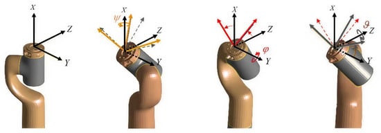
Figure 3. Rotation sequence for the end-effector.

3.2. Dynamic Model

The dynamic model provides a mathematical description that captures the behavior of a robotic system, relating the positions, velocities, accelerations, forces, and torques in its joints, along with parameters such as the masses and moments of inertia of the robot. The Euler–Lagrange dynamic equations, based on the conservation of kinetic and potential energy, are key to determining the torques generated at the rotational joints. The equations of motion written in compact matrix form representing the dynamic model of the joint space [23] are given by

$$\mathit{\tau }\left(\mathbf{t}\right)=\tilde{\mathbf{M}}\left(\mathbf{q}\left(\mathbf{t}\right)\right)\ddot{\mathbf{q}}\left(\mathbf{t}\right)+\tilde{\mathbf{C}}(\ddot{\mathbf{q}}\left(\mathbf{t}\right),\dot{\mathbf{q}}\left(\mathbf{t}\right))\dot{\mathbf{q}}\left(\mathbf{t}\right)+\tilde{\mathbf{g}}\left(\mathbf{q}\left(\mathbf{t}\right)\right)$$

(8)

where $\mathit{\tau }\left(\mathbf{t}\right)=\left[\begin{array}{cccc}{\tau }_1& {\tau }_2& \dots & {\tau }_n\end{array}\right]$ is the vector of torques and forces associated with the generalized coordinates of the robotic arm; $\ddot{\mathbf{q}}\left(\mathbf{t}\right)$ is the vector of accelerations of the robotic arm; $\tilde{\mathbf{M}}\left(\mathbf{q}\left(\mathbf{t}\right)\right)\in {\mathbb{R}}^{6\times 6}$ is the inertia matrix of the robotic arm; $\widetilde{\mathbf{C}\left(\mathbf{t}\right)}(\mathbf{q}\left(\mathbf{t}\right),\dot{\mathbf{q}\left(\mathbf{t}\right)})\in {\mathbb{R}}^{6\times 6}$ is the matrix of centripetal and Coriolis forces; $\tilde{\mathbf{g}}\left(\mathbf{q}\left(\mathbf{t}\right)\right)\in {\mathbb{R}}^6$ is the gravity vector. Therefore, it is necessary to express the dynamic model of the robotic arm in terms of reference velocities, considering that it is composed of electric servomotors [24]. The torques applied to each joint are represented in the next equation:

$${\tau }_i={\displaystyle \frac{{k_a}_i}{{r_a}_i}}\left(v_i-{k_b}_i{\dot{q}}_i\right)i=1,2,3,\dots n$$

(9)

where ${\dot{q}}_i$ corresponds to the angular velocity generated in each joint; ${k_a}_i$ represents the torque constant adjusted by the gear reduction ratio; ${r_a}_i$ is the armature resistance of the motor; ${k_b}_i$ denotes the back electromotive force (EMF) constant also scaled by the gear reduction ratio; and $v_i$ is the voltage supplied to the motor. In this context, each motor of the system is equipped with a low-level PD control that precisely adjusts the critical variables for the robot’s operation. The controller is represented by

$${\tau }_i={\displaystyle \frac{{k_a}_i}{{r_a}_i}}\left({k_p}_i{\dot{q}}_{i_{ref}}-({k_p}_i-{k_b}_i){\dot{q}}_i-{k_d}_i{\ddot{q}}_i\right)i=1,2,3,\dots n$$

(10)

where ${\dot{q}}_{i_{ref}}$ is the reference angular velocities and ${\ddot{q}}_i$ is the angular acceleration of the motors. This allows us to replace the traditional torque-based approach with a representation in terms of angular velocities, providing greater simplicity and efficiency in controlling the joints, which is presented in the next matrix:

$${\dot{\mathbf{q}}}_{\mathbf{ref}}\left(\mathbf{t}\right)=\mathbf{M}\left(\mathbf{q},\xi \right)\ddot{\mathbf{q}}\left(\mathbf{t}\right)+\mathbf{C}\left(\mathbf{q},\dot{\mathbf{q}},\xi \right)\dot{\mathbf{q}}\left(\mathbf{t}\right)+\mathbf{g}\left(\mathbf{q},\xi \right)$$

(11)

where $\ddot{\mathbf{q}}\left(\mathbf{t}\right)=\left[\begin{array}{cccc}{\ddot{q}}_1& {\ddot{q}}_2& \dots & {\ddot{q}}_n\end{array}\right]$ is the vector of accelerations of the robotic arm; $\mathbf{M}(\mathbf{q},\xi )\in {\mathbb{R}}^{\mathbf{6}\times \mathbf{6}}$ is the new inertia matrix of the robotic arm; $\mathbf{C}(\mathbf{q},\dot{\mathbf{q}})\in {\mathbb{R}}^{6\times 6}$ is the new matrix of centripetal and Coriolis forces; $\mathbf{g}\left(\mathbf{q}\right)\in {\mathbb{R}}^6$ is the new gravity vector; and $\xi =\left[\begin{array}{cccc}{\xi }_1& {\xi }_2& \dots & {\xi }_l\end{array}\right]\in {\mathbb{R}}^l$ is the vector of the dynamic parameters of the robotic arm, y l es el número de parámetros dinámicos. So the dynamic model represented in a schematic is shown in Figure 4.

Figure 4. UFactory 850 mathematical model scheme.

3.3. Control Algorithm

For the control loop implementation detailed in the schematic in Figure 5, two different control algorithms are proposed. (i) The first one is based on the inverse matrix of the process, which allows us to obtain a direct relationship between the inputs and outputs of the system. (ii) The second one uses the sliding mode control technique, which is robust to model uncertainties and external disturbances. This method ensures that the system converges to a predefined sliding surface, maintaining stable behavior even in the presence of unmodeled dynamics or variations in system parameters.

Figure 5. Control algorithm scheme.

${\mathbf{h}}_{\mathbf{d}}\left(\mathbf{t}\right)\in {\mathbb{R}}^{\mathbf{6}}$ is the vector containing the coordinates of the desired task set by the user; $\mathbf{h}\left(\mathbf{t}\right)\in {\mathbb{R}}^6$ is the vector containing the Cartesian position and orientation of the operating endpoint, set in Equation (6); $\widetilde{\mathbf{h}\left(\mathbf{t}\right)}$ is the control error, set by the difference between the desired positions and orientations with the actual positions and orientations; ${\dot{\mathbf{q}}}_{\mathbf{c}}\left(\mathbf{t}\right)$ is the vector of maneuverability velocities delivered by the proposed control algorithm; ${\dot{\mathbf{q}}}_{\mathbf{ref}}\left(\mathbf{t}\right)$ is the vector of maneuverability velocities entering the robotic arm, in which some perturbation may arise, thus entering the dynamic and kinematic model established in Section 3.

3.3.1. Reverse Process-Based Control Law

The first algorithm is the control law based on the kinematics of the robotic arm is stated in the equation

$${\dot{\mathbf{q}}}_{\mathbf{c}}\left(\mathbf{t}\right)={\mathbf{J}}^{-1}\mathbf{W}tanh\left(\alpha \tilde{\mathbf{h}}\left(\mathbf{t}\right)\right)$$

(12)

where ${\dot{\mathbf{q}}}_{\mathbf{c}}\left(\mathbf{t}\right)\in {\mathbb{R}}^6$, represents the velocities entering the robot joints; ${\mathbf{J}}^{-1}\in {\mathbb{R}}^{6\times 6}$, represents the inverse of the Jacobian matrix of the robotic arm; $\mathbf{W}\in {\mathbb{R}}^{6\times 6}$ indicates the positive definite gain matrix; $\tilde{\mathbf{h}}\left(\mathbf{t}\right)$ represents the error vector of the position and orientation of the end-effector of the robotic arm given by $\tilde{\mathbf{h}}\left(\mathbf{t}\right)={\mathbf{h}}_{\mathbf{d}}\left(\mathbf{t}\right)-\mathbf{h}\left(\mathbf{t}\right)$; in addition, the function $tanh(.)$ is used in order to limit the error with values $\alpha >0$.

For the stability analysis, a closed-loop equation is considered, which represents the behavior of the robotic arm under a proposed control algorithm; in this case, under ideal conditions, it is considered that ${\dot{\mathbf{q}}}_{\mathbf{c}}\left(\mathbf{t}\right)\equiv {\dot{\mathbf{q}}}_{\mathbf{ref}}\left(\mathbf{t}\right)$, taking into account that regulation tasks are executed ${\dot{\mathbf{h}}}_{\mathbf{d}}\left(\mathbf{t}\right)=0$. Thus, substituting Equation (12) into Equation (7), the following closed-loop equation is obtained:

$$\dot{\tilde{\mathbf{h}}}\left(\mathbf{t}\right)=-\mathbf{W}tanh\left(\alpha \tilde{\mathbf{h}}\left(\mathbf{t}\right)\right)$$

(13)

Subsequently, the Lyapunov theory was applied for stability analysis, which requires the identification of a candidate function. Since the process of defining it properly can be lengthy, it was chosen to use the mean squared error as a candidate function. From this, the evolution of the Lyapunov candidate function was derived by applying its derivative, yielding the expression $\dot{V}\left(\tilde{\mathbf{h}}\left(\mathbf{t}\right)\right)=\tilde{\mathbf{h}}{\left(\mathbf{t}\right)}^T\dot{\tilde{\mathbf{h}}}\left(\mathbf{t}\right)$. Therefore, including the closed-loop equation in the evolution of the Lyapunov candidate yields a stability analysis represented by

$$\dot{V}\left(\tilde{\mathbf{h}}\left(\mathbf{t}\right)\right)=-\tilde{\mathbf{h}}{\left(\mathbf{t}\right)}^T\mathbf{W}tanh\left(\alpha \tilde{\mathbf{h}}\left(\mathbf{t}\right)\right)<0$$

(14)

this expression ensures control loop stability, giving the end-effector position error $\tilde{\mathbf{h}}\left(t\right)\to 0$ when $t\to \infty$, resulting in an asymptotically stable system.

3.3.2. Sliding Mode Control

Sliding mode control (SMC) is a robust control technique used in dynamic systems, especially those with uncertainties or disturbances. Its basic principle is to drive the system towards a predefined sliding surface, where the system behavior becomes insensitive to perturbations and parameter variations. Once this surface is reached, the system “slides” towards the desired state, maintaining stability and accuracy even under adverse conditions.

Let $s\left(t\right)=h_d\left(t\right)-h\left(t\right)$ be the control error and $s\left(t\right)=h_d\left(t\right)-h\left(t\right)$ be the derivative of the error. $s\left(t\right)$ is a time-invariant sliding surface in n-state space, proposed by the following scalar equation for the control law:

$$s\left(t\right)={\mathbf{K}}_{\mathbf{p}}\tilde{\mathbf{h}}\left(\mathbf{t}\right)+{\mathbf{K}}_{\mathbf{i}}{\int }_0^t\tilde{\mathbf{h}}\left(\mathbf{t}\right)dt$$

(15)

where ${\mathbf{K}}_{\mathbf{p}}{\mathbf{K}}_{\mathbf{i}}\in {\mathbb{R}}^{\mathbf{6}\times \mathbf{6}}$ and ${\mathbf{K}}_{\mathbf{i}}\in {\mathbb{R}}^{\mathbf{6}\times \mathbf{6}}$ are the proportional matrix and integral matrix, respectively, both with a positive diagonal. Subsequently, using the derivative in time $\dot{s}\left(t\right)={\mathbf{K}}_{\mathbf{p}}\dot{\tilde{\mathbf{h}}}\left(\mathbf{t}\right)+{\mathbf{K}}_{\mathbf{i}}\tilde{\mathbf{h}}\left(\mathbf{t}\right)$, and considering that it is on a sliding surface, i.e., we have zero tracking error $\dot{s}=0$, we obtain

$${\mathbf{K}}_{\mathbf{p}}\dot{\tilde{\mathbf{h}}}\left(\mathbf{t}\right)+{\mathbf{K}}_{\mathbf{i}}\tilde{\mathbf{h}}\left(\mathbf{t}\right)=0;$$

(16)

substituting the derivative of the control error and taking into account that the model is represented by Equation (6) results in $\mathbf{Kp}(\dot{{\mathbf{h}}_{\mathbf{d}}}\left(\mathbf{t}\right)-\mathbf{J}\dot{\mathbf{q}}\left(\mathbf{t}\right))+\mathbf{Ki}\tilde{\mathbf{h}}\left(\mathbf{t}\right)=\mathbf{0}$; therefore, the continuous part of the controller is represented by the following equation:

$${\dot{\mathbf{q}}}_{\mathbf{con}}\left(\mathbf{t}\right)={\mathbf{K}}_{\mathbf{p}}^{-\mathbf{1}}{\mathbf{J}}^{-\mathbf{1}}({\mathbf{K}}_{\mathbf{p}}{\dot{\mathbf{h}}}_{\mathbf{d}}\left(\mathbf{t}\right)+{\mathbf{K}}_{\mathbf{i}}\tilde{\mathbf{h}}\left(\mathbf{t}\right))$$

(17)

where ${\dot{\mathbf{h}}}_{\mathbf{d}}$ is the derivative of the desired task. On the other hand, the discontinuous part is expressed by the equation

$${\dot{\mathbf{q}}}_{\mathbf{dis}}\left(\mathbf{t}\right)={\mathbf{J}}^{-\mathbf{1}}{\mathbf{K}}_{\mathbf{p}}^{-\mathbf{1}}\mathbf{F}\left(s\right)$$

(18)

where $\mathbf{F}\left(\mathbf{s}\right)$ is the discontinuous part of the controller, designed to apply a control action that drives the system towards the sliding surface. This function is defined by Equation (19):

$$\mathbf{F}\left(s\right)={\displaystyle \frac{s\left(t\right)}{\gamma +\parallel s\left(t\right)\parallel }}$$

(19)

where $\gamma$ is a gain that controls the amplitude of the discontinuous part of the controller, and $\mathbf{S}$ represents the sliding surface in sliding mode control. Finally, the resulting control law is defined as

$${\dot{\mathbf{q}}}_{\mathbf{c}}={\dot{\mathbf{q}}}_{\mathbf{con}}\left(\mathbf{t}\right)+{\dot{\mathbf{q}}}_{\mathbf{dis}}\left(\mathbf{t}\right)$$

(20)

where ${\dot{\mathbf{q}}}_{\mathbf{c}}\in R^6$ represents the joint velocities of the robot. Therefore, for the stability analysis, a closed-loop equation is considered. In this case too, it is considered that ${\dot{\mathbf{q}}}_{\mathbf{c}}={\dot{\mathbf{q}}}_{\mathbf{ref}}$, taking into account that regulation tasks are executed ${\dot{\mathbf{h}}}_d=0$. Taking into account Equation (20), the following closed-loop equation is obtained:

$$\dot{s}\left(t\right)={\mathbf{K}}_{\mathbf{p}}{\dot{\mathbf{h}}}_{\mathbf{d}}\left(\mathbf{t}\right)-{\mathbf{K}}_{\mathbf{p}}\mathbf{J}{\dot{\mathbf{q}}}_{\mathbf{c}}\left(\mathbf{t}\right)+{\mathbf{K}}_{\mathbf{i}}\tilde{\mathbf{h}}\left(\mathbf{t}\right)$$

(21)

now, by replacing Equation (21), Lyapunov’s theory was applied for stability analysis, again using the mean square error, and establishing the Lyapunov equation as $V\left(\mathbf{S}\right)={\mathbf{S}}^T\mathbf{S}$, resulting in the equation

$$\dot{\mathbf{V}}\left(s\right)=-s^T\left({\mathbf{K}}_{\mathbf{p}}\mathbf{J}{\dot{\mathbf{q}}}_{\mathbf{dis}}\left(\mathbf{t}\right)\right)<\mathbf{0}$$

(22)

considering Equation (18) for the controller design, it is found that the control error ${\displaystyle \underset{t\to \infty }{lim}\tilde{\mathbf{h}}=0}$, resulting in an asymptotically stable system.

4. Virtualization of the Environment

This section presents the virtualization of the virtual training system, as shown in Figure 6. The full simulation is performed using Unity3D software, which provides a detailed and realistic three-dimensional environment for the training of the UFACTORY robot, including the creation of interactive scenes and scripts with the mathematical model of the robot to simulate and give more realism to the environment. In addition, MATLAB is used to perform a simulation of the controller, in which the proposed control algorithm is executed. Although MATLAB allows effective validation of the control with its ability to handle complex calculations, its graphical capabilities are more limited.

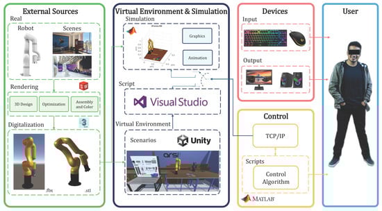
Figure 6. Schematic of the virtualization of the Ufactory 850 robot and the scenes required for an immersive virtual training system.

When virtualizing the system, two main files are generated: one for the interactive environment in Unity and another for the simulation in MATLAB. The graphical simulation in MATLAB includes the ability to animate the robot in basic graphics, while Unity provides an advanced visual representation.

For the virtualization of the system, several external resources were used, including different scenarios, as well as the industrial robot Ufactory 850. The robot design was implemented in the CAD modeling software SolidWorks ver. 2023. From this design, an STL file was created in 3DS Max software, which was used for simulation in MATLAB, adjusting the reference axes of the robot’s joints. In addition, the STL file was converted to FBX format, which was necessary to integrate it into the Unity graphics engine. The exported models were assembled in their respective software, as shown in Figure 7.

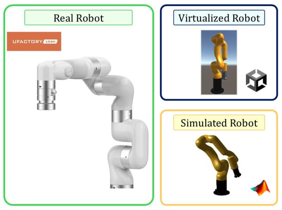
Figure 7. Virtualization of the Ufactory 850 robot on Matlab and Unity.

Additionally, the Unity 3D engine can be used to develop various environments that are part of the virtual training system, such as a research laboratory, an industrial setting represented by an assembly line, and a service environment simulating a bar. Digitized in FBX format, these environments focus on the field of service and industrial robotics, making them highly useful for the teaching and learning process, facilitating robot interaction in performing position tasks assigned by the user.

The programming scripts in Unity include lines of code that emulate the movement of the UFactory robot, generated through the mathematically derived model, both kinematic and dynamic. Additionally, other scripts have been added for animation, fault management, and other objects. A menu scene has also been incorporated into the Unity environment, allowing the user to switch between different scenes at will, enhancing flexibility and navigation within the virtual training system.

Channel Communication

Figure 8 illustrates the information exchange scheme between MATLAB and Unity3D, implemented via the TCP/IP protocol in a communication environment facilitated by ROS (Robot Operating System). This protocol enables real-time data transmission and reception, facilitating bidirectional communication between MATLAB and Unity or MATLAB and the robot in real time [25]. In this system, MATLAB contains the main control algorithm, where it receives the robot’s joint states and generates the necessary control actions. These actions are sent to Unity via ROS, where programming scripts process the received data and update the position and orientation of the robotic model in the graphical environment. Thus, Unity receives the information from MATLAB and simulates the robot’s movement in the virtual environment, providing an intuitive and realistic visualization environment that allows the user to interact with the model and observe the effect of the control actions in real time.

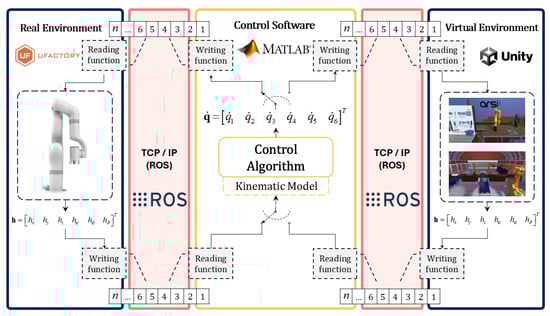
Figure 8. Communication system configuration between virtual environment and control algorithm.

Additionally, after completing the use of the virtual training system, the same control algorithm can be implemented on the UFactory 850 robot without requiring additional modifications. Communication between the control software and the physical robot is efficiently carried out through the TCP/IP protocol, enabling the rapid and precise transfer of commands and control data. Similar to the training system, the control algorithm receives the positions and orientations of the end-effector to calculate the necessary control actions for each joint. These actions are then transmitted to the robot, ensuring precise and coordinated movement according to the established parameters. This integration ensures a seamless transition from the simulator to the real robot, facilitating the practical validation of the algorithms developed in the virtual environment. This guarantees that users can test and adjust their algorithms in a safe environment before applying them directly to the physical robot, reducing risks and improving the reliability of the results.

The integration of ROS into this architecture not only facilitates information exchange but also enables the system to be expanded to include other simulation and control modules, providing greater flexibility in the design of robotics applications and optimizing the simulation process.

5. Result Analysis

This section outlines the results derived from the basic simulation of the control loop for the UFactory xArm 5 robotic arm in Matlab, alongside the virtual environment simulation in Unity. Furthermore, it incorporates an experimental validation phase, where the simulated robotic arm’s performance is rigorously compared against the real-world robotic system. This validation process ensures the fidelity of the simulation by evaluating its alignment with the physical robot under identical operational conditions. It should be noted that in the simulation cases, in both cases, the hardware used includes an Intel(R) Core(TM) i7-11800H processor of 11th generation at 2.30 GHz (8 cores) and a GeForce RTX 3060 graphics card. Although the behavior of the virtualized robotic system is not strictly hardware-dependent, its use is recommended to ensure smooth animation of the virtual environment.

5.1. Matlab Simulation

For the simulation performed in a MATLAB software script, a task of positioning various parts was carried out with the aim of moving each object from one position to another. In this simulation, the virtualized UFactory 850 robot in .STL format was used, as described in Section 4, and the control laws specified in Equations (12) and (20) were applied. The desired points consist of a set of coordinates that define the position and orientation of the objects and the locations of the operating endpoint $({\mathbf{h}}_{\mathbf{d}}\left(\mathbf{t}\right)\in {\mathbb{R}}^{\mathbf{6}})$, from the moment it picks up the object until it reaches the next point. These points are arranged in a specific order to avoid collisions. The points are entered by the user, and the simulation process is illustrated in Figure 9. In this case, in order for the algorithm to continuously change the coordinates of the desired point, a parameter was assigned based on the norm of the error vector, which must be less than $\left|\right|\tilde{\mathbf{h}}\left(\mathbf{t}\right)\left|\right|=\sqrt{{\tilde{h}}_x^2+{\tilde{h}}_y^2+{\tilde{h}}_z^2+{\tilde{h}}_{\psi }^2+{\tilde{h}}_{\phi }^2+{\tilde{h}}_{\vartheta }^2}=0.02$ [m], with $\tilde{\mathbf{h}}\left(\mathbf{t}\right)$ [m], where $\mathbf{h}\left(\mathbf{t}\right)$ is the difference between the desired positions and orientations, with the actual positions and orientations.

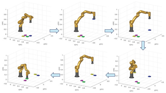
Figure 9. Stroboscopic movement of the Matlab simulation.

To evaluate the behavior of the robotic system and the proposed control algorithm, the evolution of the control errors in each of the rectangular coordinates of $x,y$ and z space, as well as in the orientation of the end-effector $\vartheta ,\phi ,$ and $\psi$, is considered, forming the vector $\tilde{\mathbf{h}}\left(\mathbf{t}\right)\in {\mathbb{R}}^{\mathbf{6}}$. These errors are plotted graphically in Figure 10, where it can be seen that the errors tend to decrease each time the operating end reaches a desired point. Subsequently, the desired point is updated to the next when $\left|\right|\tilde{\mathbf{h}}\left|\right|=\mathbf{0}.\mathbf{02}$ m, allowing the system to adjust its position and orientation continuously and accurately.

Figure 10. Control errors of the final effector in Matlab software with $\tilde{\mathbf{h}}\left({\tilde{h}}_x{\tilde{h}}_y{\tilde{h}}_z{\tilde{h}}_{\psi }{\tilde{h}}_{\phi }{\tilde{h}}_{\vartheta }\right)$.

As shown in Figure 10, the proposed control algorithms correctly perform the desired task; however, the SMD controller tends to perform better compared to its counterpart RPBCL. Therefore, in Figure 11, the error norm is presented in each of the time intervals present in the simulation.

Figure 11. Evolution of the error norm as a function of time for control algorithms.

With this, it can be established that the SMD algorithm tends to have a better response to disturbances, both internal and external, that affect the robotic arm. This robustness is due to its ability to efficiently handle the dynamic variations and uncertainties of the system, which allows it to maintain a high level of accuracy and stability in trajectory tracking.

5.2. Virtual Environment

The immersive virtual environment for teaching and learning starts with a menu that displays information about its design and offers the possibility to select one of the three available scenes for the simulation of the UFactory 850 robot: a laboratory, a bar for the service robotics simulation, and an assembly line for the industrial environment. The user can choose the desired scene, and Figure 12 illustrates the menu.

Figure 12. Virtual environment menu.

5.2.1. Laboratory Scene

The first scene recreates the physical environment of the laboratory where the UFactory 850 robot is located, with the objective of executing pick and place tasks of specific objects, in this case, plastic containers. The user or student defines the location of the containers within the work area of the robotic arm; with this, the virtual environment determines the desired position and orientation $({\mathbf{h}}_{\mathbf{d}}\left(\mathbf{t}\right)\in {\mathbb{R}}^{\mathbf{6}})$. Subsequently, the robot automatically arranges the garbage cans, similar to the MATLAB simulation (Section 5.1). However, by using a graphics engine, the simulation acquires a higher level of realism, as the visual representation is more detailed and closely resembles the real environment, incorporating elements present in the physical laboratory. This is illustrated in the images in Figure 13. In addition, the student has the possibility to interact with the environment by moving around the entire laboratory, as well as adjust the required precision in the placement of objects and the sequence of tasks. This allows the user to understand how these parameters affect the robot’s performance and task efficiency. The option to visualize control errors in real time is also included, which facilitates analysis and debugging of the system.

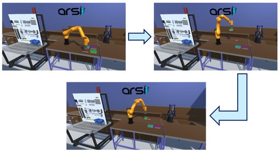
Figure 13. Ufactory 850 in the virtual laboratory scene.

For the demonstration of this scene, a screen showing the control errors when executing the desired task is included in the virtual environment, as shown in Figure 14. This screen shows the errors in the Cartesian coordinates x, y and z, as well as the orientation errors $\vartheta$, $\phi$ and $\psi$$(\tilde{\mathbf{h}}\left(\mathbf{t}\right)\in {\mathbb{R}}^{\mathbf{6}})$, which are remarkably similar to those shown in the graph in Figure 10.

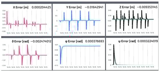
Figure 14. Control errors of the final effector in Unity.

5.2.2. Bar Scene

For the service robotics approach, a bar scene was designed to simulate the preparation of a cocktail. In this environment, the robot executes bottle positioning and manipulation tasks. For this case, the end-effector was replaced by a gripper instead of a suction cup, using an ON/OFF control to grasp and release objects. In this simulation, the force sensor feedback present on the actual UFactory 850 robot was not considered. Figure 15 illustrates the task performed by the robotic arm. In this scenario, the user selects the bottles to be used for cocktail preparation within the virtual environment, thus defining the position and orientation of the desired points $({\mathbf{h}}_{\mathbf{d}}\left(\mathbf{t}\right)\in {\mathbb{R}}^{\mathbf{6}})$ for the control algorithm. From this sequence of points, the robot executes the cocktail preparation task, transferring the liquid from the bottles to the glass located on the table. In addition, the student can experiment with different grip configurations and adjust the sequence of steps for preparing the cocktail. This allows the user to explore how these factors influence the efficiency of the task and the accuracy of the robot. The option to simulate common errors, such as spilling liquids if the desired spot on the glass is not correctly positioned, is also provided so that the student can learn to identify and correct these problems.

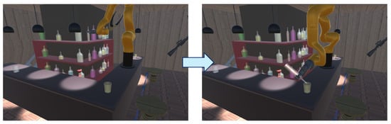
Figure 15. Ufactory 850 in the virtual bar scene.

5.2.3. Assembly Scene

For the industrial approach, a sheet metal positioning task was developed, in which the UFactory 850 robot is in a fixed position to move and rotate the sheets between two conveyor belts for subsequent packaging. The end-effector of the robot is again a suction cup. The user can define the coordinates of the sheet metal as desired points and has the option of placing it on the conveyor belt to the left of the robot arm (for finished products) or on the belt to the right (for damaged products). This decision is entirely up to the user, who will enter the desired points for the execution of the task in the Matlab software. The simulation of this scene is presented in Figure 16. Additionally, the student can adjust parameters such as the speed of the conveyor belts, and the precision required in the positioning of the sheets. This allows the user to understand how these factors affect the efficiency of the industrial process and the quality of the final product. The possibility of simulating failures in the system, such as the slipping of the sheets, is also included so that the student can learn to solve these problems in a controlled environment.

Figure 16. Ufactory 850 in the virtual assembly industrial scene.

5.3. Experimental Validation

In this section, a comparison is made between two scenes in the virtual environment and two real applications using the UFactory 850 robot in the research and robotics laboratory of the Universidad de las Fuerzas Armadas ESPE. The first scene is a pick and place process of plastic containers, which is presented both in the virtual environment of the laboratory and in its real counterpart, using the same objects. Users operate the UFactory 850 after prior training with the teaching–learning tool, achieving a successful execution of the task without presenting problems when replicating it in the physical environment. This is illustrated in the images in Figure 17.

Figure 17. Comparison between the performance of Ufactory 850 positioning tasks in the real laboratory and the virtual laboratory.

In the service robotics scene, the objective is to prepare a cocktail with various elements, for which a pick and place task is performed, and various desired points, using a gripper as the final effector for gripping the objects. In this case, the user enters the desired points of each of the objects to execute the control loop and the UFactory robot performs the desired task. In this case, the Ufactory robot approaches the bottle at various points, and when it is close, it grabs the bottle and moves towards the place where the glass is located by means of various desired points to avoid spilling the liquid from the bottle or any collision; subsequently, when it reaches the place, the end-effector rotates with the aim of spilling the liquid into the glass, which is the desired task.

To demonstrate the reliability of the communication channel, Figure 18 shows how long it takes the machine to process each iteration in calculating the error and sending the corresponding control actions, where clearly the first error always takes the longest, while for the rest, the average is the sampling time, thus maintaining real-time communication.

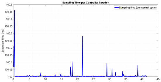
Figure 18. Control loop sampling time performance.

Quantitative Comparison and Robustness Evaluation

To quantify the fidelity of the Digital Twin and the robustness of the control algorithms, each scenario (laboratory, service, and industrial) was run ten times for each control strategy, reverse process-based control law (RPBCL) and sliding mode control (SMC), using identical initial configurations and task sequences in both the simulation and physical execution to ensure a fair comparison. The average RMS position error between simulation and actual execution was 1.8 mm ± 0.4 mm for RPBCL and 1.4 mm ± 0.3 mm for SMC, while the average RMS orientation error was 0.9° ± 0.2° for RPBCL and 0.7° ± 0.2° for SMC. A paired t-test revealed no statistically significant differences between simulation errors and actual execution errors (p > 0.05), confirming the high fidelity of the Digital Twin. When analyzed by scenario, the laboratory environment showed RMS position errors not exceeding 1.6 mm and orientation errors of less than 0.8°, the service environment recorded position errors of up to 1.9 mm and orientation errors of up to 0.9°, and the industrial environment showed position errors of up to 2.0 mm and orientation errors of up to 1.0°, with a slight increase attributable to the greater complexity of the task. Under a controlled disturbance of ±0.02 Nm applied to the joints, the SMC maintained maximum position deviations of 2.1 mm, representing a 15% reduction compared to the RPBCL, while orientation deviations remained at 0.9° for the SMC versus 1.1° for the RPBCL, and recovery times to the desired trajectory were reduced by 14% to 17% with the SMC. These results confirm that the proposed dynamic symmetry preservation model, combined with torque-to-velocity translation and robust sliding mode control, provides consistent tracking accuracy across all scenarios, strong disturbance rejection, and minimal discrepancy between simulated and actual performance.

As can be seen in Figure 19, the dynamic responses show a remarkable similarity between the simulated speed signals (green) and those of the actual robot (red). This close parallelism demonstrates the high fidelity of the proposed model in replicating the actual behavior of the robot. The minimal discrepancies observed remain within acceptable margins of error, confirming the accuracy and reliability of the model for its implementation in control design and system analysis. Despite this agreement, the fidelity of the model could be improved for tasks requiring greater precision through parameter identification techniques, which constitutes a promising line of future work. These results validate the simulation methodology employed and indicate excellent predictive capability for practical applications.

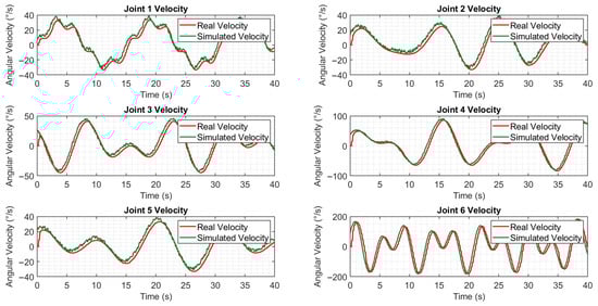
Figure 19. Comparison between real robot and robot simulated with velocity signals.

In Figure 20, the performance comparison of the UFactory 850 manipulator executing positioning tasks is presented in both a real physical environment (real bar) and a virtual simulated environment (digital bar). This parallel validation establishes the correspondence between the digital twin and the physical robot, confirming that the virtual environment accurately reproduces the reaching and placement motions carried out in the real platform. Furthermore, the digital model preserves the kinematic characteristics, motion trajectories, and precision levels required for robotic service applications. This correspondence not only validates the digital twin as a tool for experimentation and verification, but also highlights its potential for cost reduction, prior evaluation of control strategies, and task optimization before deployment in real scenarios.

Figure 20. Comparison between the performance of Ufactory 850 positioning tasks in the real bar and the virtual bar for the robotic services.

5.4. Evaluation of the Training Tool

To evaluate the effectiveness of the training tool, a test was conducted to measure understanding of the tool, knowledge of robotics, and ease of learning. The test was applied to 20 students from the Universidad de las Fuerzas Armadas ESPE, who had basic knowledge in robotics and virtual environments, both before and after using the tool together with the real robot. The questionnaire consisted of 10 questions with quantitative answers, presented in Table 2, using a scale from 0 to 5, where 0 indicates the lowest level of understanding and 5 the highest.

Table 2. List of questions.

Ord.	Questions
1	How clear did you find it to visualize the robot’s movements before and after using the tool?
2	How would you rate the accuracy in simulating the robot’s behavior before and after using the tool?
3	How easy was it for you to understand the kinematics and dynamics of the robot before and after using the tool?
4	How capable did you feel you were in identifying errors in the programming before and after using the tool?
5	How well did you understand the interaction between the robot hardware and the control software before and after using the tool?
6	How confident did you feel in applying the acquired knowledge in a physical environment after using the tool?
7	How satisfied were you with the user interface before and after using the tool?
8	How prepared were you to work autonomously in simulations before and after using the tool?
9	How motivated did you feel to continue learning robotics after using the tool?
10	How easy was it for you to use the virtual environment tool before and after use?

Based on the questions in Table 2, the average answers for each question are presented in Table 3. In addition, a spider web graph is included that more clearly illustrates the results of the test, comparing users’ perceptions before and after using the tool and the physical robotic arm. This graph reveals a significant difference between the scores obtained before and after the intervention, depicted in Figure 21.

Table 3. Comparison of scores before and after using the training tool.

Aspect Evaluated	Before (Average)	After (Average)
Clarity in Robotic Movement Visualization	2.8	4.3
Accuracy in Behavior Simulation	3.0	4.5
Ease of Understanding Kinematics and Dynamics	2.7	4.2
Ability to Identify Programming Errors	2.5	4.1
Understanding of Hardware–Software Interaction	2.6	4.0
Confidence in Application in Real Environments	2.3	4.4
Satisfaction with User Interface	3.1	4.6
Ability to Work Independently	2.9	4.3
Level of Motivation to Continue Learning	3.2	4.7
Ease of Use of the Virtual Environment	3.0	4.5

Figure 21. Evaluation of student performance using the virtual learning tool before and after its use.

In the spider graph presented in Figure 21, the results of the comprehension levels present in the students before and after the use of this e-learning tool are visualized. In questions 1, 2, 3, 7, 9 and 10, there is a difference of 1.5 points before vs. after the use of this e-learning tool. In questions 5 and 8, there is a difference of 1.4 between the before and after scores. In the fourth question, the difference between these times is 1.6 points, and finally, the sixth question presents a greater difference of 2.1 points, showing that this tool gave them greater confidence in the application in real environments.

Taken together, these data indicate that there is a significant improvement after using this program. The differences in the scores suggest that the e-learning tool is very important for the students’ learning development as it gives them confidence to apply this knowledge in a more practical situation.

6. Discussion

This paper presents the mathematical model of the UFactory 850 robotic arm, based on its kinematic and dynamic characteristics. which has proven fundamental both for generating realistic simulations in Unity and for the design of precise and robust control algorithms [26]. Unlike conventional approaches, the proposed model explicitly identifies and preserves geometric, kinematic, and dynamic symmetries in the manipulator structure. From a theoretical perspective, these symmetries can be interpreted as invariants under specific transformations in configuration space, which simplify the underlying equations of motion. In practice, their exploitation reduces computational load, improves numerical stability, and ensures consistent control performance across equivalent joint configurations.

The symmetry present in the robot’s design has facilitated the formulation of generalizable models that can be adapted to different control strategies and operating scenarios. This property simplifies the modeling process and strengthens the scalability of the simulation framework, in contrast to previous works that do not explicitly exploit this structural feature [27,28]. Likewise, the integration of MATLAB for developing and tuning control algorithms together with Unity for immersive simulation has resulted in a highly effective validation environment, which demonstrates fidelity between simulation and physical execution.

The quantitative results obtained reinforce this claim. Across multiple repetitions in different scenarios, the symmetry-preserving control framework exhibited RMS position errors below 1.8 mm and orientation errors under 1°, with no statistically significant differences between simulation and real execution. Furthermore, under controlled disturbances, the sliding mode control consistently outperformed the inverse process law, reducing deviations and recovery times by up to 17% without compromising stability. These outcomes validate the effectiveness of the proposed model in terms of accuracy and robustness.

The developed virtual environment also provides a safe and versatile space for experimentation, allowing the exploration of extreme configurations and the validation of algorithms under conditions that would be risky or costly to reproduce physically. Unlike studies focused exclusively on hardware testing or theoretical models disconnected from practice, this research proposes a hybrid Digital Twin solution that, by leveraging the structural symmetry of the robot, enables predictive simulation and early validation of control algorithms. Compared to vision-based approaches, such as that of Shahria et al. [13], our method removes the dependency on optical feedback, achieving precise trajectory tracking and effective disturbance rejection even in environments where cameras cannot be reliably deployed.

In this context, the integration of mathematical modeling, control algorithm design, and immersive simulation based on symmetry constitutes a comprehensive framework for the validation of robotic systems. The results confirm that symmetry is not merely a geometric convenience but a strategic advantage that enhances control accuracy, simulation fidelity, and development efficiency.

7. Conclusions

This study demonstrates that preserving symmetries in the dynamic modeling of the UFactory 850 enables the creation of a precise and robust Digital Twin, capable of reproducing real robot operation with high fidelity while supporting the design of advanced control algorithms. By integrating symmetry-preserving modeling, robust sliding-mode control, and immersive simulation, the proposed framework ensures accuracy, robustness, and scalability, offering advantages over conventional approaches that overlook structural symmetries. Although validated on the UFactory 850, the methodology provides a transferable basis for extending Digital Twin applications to other robotic platforms, as well as to future research in cooperative multi-robot control and the management of dynamic asymmetries such as variable loads, paving the way toward resilient robotic systems for complex and high-demand operational scenarios.

References

- Ghaffari, M.; Zhang, R.; Zhu, M.; Lin, C.E.; Lin, T.Y.; Teng, S.; Li, T.; Liu, T.; Song, J. Progress in Symmetry Preserving Robot Perception and Control Through Geometry and Learning. Front. Robot. AI 2022, 9, 969380. [Google Scholar] [CrossRef]
- Granić, A. Educational Technology Adoption: A Systematic Review. Educ. Inf. Technol. 2022, 27, 9725–9744. [Google Scholar] [CrossRef]
- Barbosa, W.S.; Gioia, M.M.; Natividade, V.G.; Wanderley, R.F.; Chaves, M.R.; Gouvea, F.C.; Gonçalves, F.M. Industry 4.0: Examples of the Use of the Robotic Arm for Digital Manufacturing Processes. Int. J. Interact. Des. Manuf. (IJIDeM) 2020, 14, 1569–1575. [Google Scholar] [CrossRef]
- Torres Martín, A.C. Impact on the Virtual Learning Environment Due to COVID-19. Sustainability 2021, 13, 582. [Google Scholar] [CrossRef]
- Ortiz, J.S.; Quishpe, E.K.; Sailema, G.X.; Guamán, N.S. Digital Twin-Based Active Learning for Industrial Process Control and Supervision in Industry 4.0. Sensors 2025, 25, 2076. [Google Scholar] [CrossRef]
- Andone, D.; Ternauciuc, A.; Vasiu, R. Using Open Education Tools for a Higher Education Virtual Campus. In Proceedings of the 2017 IEEE 17th International Conference on Advanced Learning Technologies (ICALT), Timisoara, Romania, 3–7 July 2017; pp. 26–30. [Google Scholar] [CrossRef]
- Kim, J. Learning and Teaching Online During COVID-19: Experiences of Student Teachers in an Early Childhood Education Practicum. Int. J. Early Child. 2020, 52, 145–158. [Google Scholar] [CrossRef]
- Joia, L.A.; Lorenzo, M. Zoom In, Zoom Out: The Impact of the COVID-19 Pandemic in the Classroom. Sustainability 2021, 13, 2531. [Google Scholar] [CrossRef]
- Ortiz, J.S.; Pila, R.S.; Yupangui, J.A.; Rosales, M.M. Interactive Teaching in Virtual Environments: Integrating Hardware in the Loop in a Brewing Process. Appl. Sci. 2024, 14, 2170. [Google Scholar] [CrossRef]
- Thanyadit, S.; Punpongsanon, P.; Piumsomboon, T.; Pong, T.C. XR-LIVE: Enhancing Asynchronous Shared-Space Demonstrations with Spatial-temporal Assistive Toolsets for Effective Learning in Immersive Virtual Laboratories. Proc. ACM Hum.-Comput. Interact. 2022, 6, 136:1–136:23. [Google Scholar] [CrossRef]
- Hernández-de Menéndez, M.; Vallejo Guevara, A.; Tudón Martínez, J.C.; Hernández Alcántara, D.; Morales-Menendez, R. Active Learning in Engineering Education: A Review of Fundamentals, Best Practices and Experiences. Int. J. Interact. Des. Manuf. (IJIDeM) 2019, 13, 909–922. [Google Scholar] [CrossRef]
- Sypsas, A.; Kalles, D. Virtual Laboratories in Biology, Biotechnology and Chemistry Education: A Literature Review. In Proceedings of the 22nd Pan-Hellenic Conference on Informatics (PCI ’18), Athens, Greece, 29 November–1 December 2018; pp. 70–75. [Google Scholar] [CrossRef]
- Shahria, M.T.; Ghommam, J.; Fareh, R.; Rahman, M.H. Vision-Based Object Manipulation for Activities of Daily Living Assistance Using Assistive Robot. Automation 2024, 5, 68–89. [Google Scholar] [CrossRef]
- Gavilanes-Sagnay, F.; Loza-Aguirre, E.; Echeverria-Carrillo, C.; Jacome-Viera, H. Virtual Learning Environments: A Case of Study. In Proceedings of the International Conference on Applied Technologies, Virtual, 27–29 October 2021; Springer: Berlin/Heidelberg, Germany, 2021; pp. 108–120. [Google Scholar]
- Aguayza, A.; Chuquizala, C.; Rendón-Enriquez, I.; Tirado-Espín, A.; Almeida-Galárraga, D. Methodological Actions for the Electronic Configuration of the Educa Plus Platform: Promoting Interactive Learning. In Proceedings of the 18th Latin American Conference on Learning Technologies (LACLO 2023); Berrezueta, S., Ed.; Springer: Singapore, 2023; pp. 116–130. [Google Scholar] [CrossRef]
- Erdogan, R.; Saglam, Z.; Cetintav, G.; Karaoglan Yilmaz, F.G. Examination of the Usability of Tinkercad Application in Educational Robotics Teaching by Eye Tracking Technique. Smart Learn. Environ. 2023, 10, 27. [Google Scholar] [CrossRef]
- Banda, H.J.; Nzabahimana, J. The Impact of Physics Education Technology (PhET) Interactive Simulation-Based Learning on Motivation and Academic Achievement Among Malawian Physics Students. J. Sci. Educ. Technol. 2023, 32, 127–141. [Google Scholar] [CrossRef] [PubMed]
- Bakhshalipour, M.; Gibbons, P.B. Agents of Autonomy: A Systematic Study of Robotics on Modern Hardware. Proc. ACM Meas. Anal. Comput. Syst. 2023, 7, 43:1–43:31. [Google Scholar] [CrossRef]
- Nedic, Z.; Machotka, J.; Nafalski, A. Remote Laboratories versus Virtual and Real Laboratories. In Proceedings of the 33rd Annual Frontiers in Education Conference (FIE 2003), Westminster, CO, USA, 5–8 November 2003; Volume 1, p. T3E. [Google Scholar] [CrossRef]
- Mo, F.; Rehman, H.U.; Chaplin, J.C.; Sanderson, D.; Ratchev, S. Digital twin-based self-learning decision-making framework for industrial robots in manufacturing. Int. J. Adv. Manuf. Technol. 2025, 139, 221–240. [Google Scholar] [CrossRef]
- Wang, D.; Park, J.Y.; Sortur, N.; Wong, L.L.; Walters, R.; Platt, R. The Surprising Effectiveness of Equivariant Models in Domains with Latent Symmetry. arXiv 2022, arXiv:2211.09231. [Google Scholar] [CrossRef]
- Sung, M.; Choi, Y. Algorithmic Modified Denavit–Hartenberg Modeling for Robotic Manipulators Using Line Geometry. Appl. Sci. 2025, 15, 4999. [Google Scholar] [CrossRef]
- Falkenhahn, V.; Mahl, T.; Hildebrandt, A.; Neumann, R.; Sawodny, O. Dynamic Modeling of Bellows-Actuated Continuum Robots Using the Euler–Lagrange Formalism. IEEE Trans. Robot. 2015, 31, 1483–1496. [Google Scholar] [CrossRef]
- Carvajal, C.P.; Andaluz, G.M.; Andaluz, V.H.; Roberti, F.; Palacios-Navarro, G.; Carelli, R. Multitask Control of Aerial Manipulator Robots with Dynamic Compensation Based on Numerical Methods. Robot. Auton. Syst. 2024, 173, 104614. [Google Scholar] [CrossRef]
- Safeea, M.; Neto, P. KUKA Sunrise Toolbox: Interfacing Collaborative Robots with MATLAB. IEEE Robot. Autom. Mag. 2019, 26, 91–96. [Google Scholar] [CrossRef]
- Pantusin, F.J.; Carvajal, C.P.; Ortiz, J.S.; Andaluz, V.H. Virtual Teleoperation System for Mobile Manipulator Robots Focused on Object Transport and Manipulation. Technologies 2024, 12, 146. [Google Scholar] [CrossRef]
- Gold, T.; Völz, A.; Graichen, K. Model Predictive Interaction Control for Robotic Manipulation Tasks. IEEE Trans. Robot. 2022, 39, 76–89. [Google Scholar] [CrossRef]
- Yin, H.; Varava, A.; Kragic, D. Modeling, learning, perception, and control methods for deformable object manipulation. Sci. Robot. 2021, 6, eabd8803. [Google Scholar] [CrossRef] [PubMed]
Disclaimer/Publisher’s Note: The statements, opinions and data contained in all publications are solely those of the individual author(s) and contributor(s) and not of MDPI and/or the editor(s). MDPI and/or the editor(s) disclaim responsibility for any injury to people or property resulting from any ideas, methods, instructions or products referred to in the content. |
© 2025 by the authors. Licensee MDPI, Basel, Switzerland. This article is an open access article distributed under the terms and conditions of the Creative Commons Attribution (CC BY) license (https://creativecommons.org/licenses/by/4.0/).