Portfolio Optimization with Multi-Trend Objective and Accelerated Quasi-Newton Method

Abstract

We propose a portfolio optimization method with a multi-trend objective and an accelerated quasi-Newton method (MTO-AQNM). It leverages a BFGS-based quasi-Newton algorithm and incorporates an ${\ell }^1$ regularization term and the self-funding constraint. The MTO is designed to identify multiple trend reversals. Different trend reversals are asymmetric, and we hoped to extract rich and effective information from them. The AQNM adopts the BFGS method with the Wolfe conditions, which reduces computational complexity and improves convergence speed. We wanted to evaluate the performance of our algorithm through financial markets that were asymmetric in all respects. To this end, we conducted comprehensive experimental approaches on six benchmark data sets of real-world financial markets that were asymmetric in time, frequency, and asset type. Our method demonstrated superior performance over other state-of-the-art competitors across several mainstream evaluation metrics.

1. Introduction

The mean variance (MV) portfolio optimization (PO) theory [1] is designed to identify an optimal investment allocation strategy that simultaneously maximizes the expected return and minimizes risk. With the accelerated advancements in machine learning and artificial intelligence, machine learning has emerged as a crucial component in quantitative investing [2]. As we all know, financial markets are characterized by a high degree of information asymmetry, and this asymmetry affects the effectiveness and efficiency of the market. Based on this, some researchers have utilized time series information to improve portfolio performance [3], an agent-based co-evolutionary multi-objective algorithm for PO [4], and uncertain stochastic control systems in portfolios [5]. These not only exploit computational capability but also mitigate the problems of human subjectivity and information asymmetry, thus improving the accuracy of forecasting results.

PO methods can be generally categorized into two approaches: the MV approach and the exponential growth rate (EGR) approach [2], each with distinct theoretical foundations, trading logic, optimization techniques, and objectives. The EGR approach, inspired by Kelly’s criterion in information theory [6], primarily concentrates on the dynamics of wealth over time. The MV approach is model-driven and often requires strict statistical assumptions about asset returns, such as accepting appropriate statistical distributions [7,8], independence between different trading periods [9], and a stationary market [10]. In contrast, the EGR approach is typically data-driven, emphasizing how to use newly emerged samples to update and enhance the investment portfolio [2]. While considering the portfolio return, it pays more attention to the exponential growth of the portfolio, not just the average return. On the other hand, the EGR approach is more robust against errors in parameter estimation. Therefore, in terms of controlling risk and market uncertainty, the performance of the EGR approach is often better than the MV approach in short-term PO.

In real-world financial environments, the price relatives ${\left\{{\mathbf{x}}_t\right\}}_{t=1}^T$ (defined in Equation (1)) may show instability, and strict statistical assumptions about asset returns may not always hold. To address these challenges, some heuristic investing strategies based on behavioral finance have been proposed [11,12,13]. There are three widely recognized trend representation strategies: trend reversing [14,15,16], trend following [17,18,19], and trend pattern matching [20]. The trend-reversing strategy assumes that asset prices will return to their historical levels in the near future. For example, the passive-aggressive mean reversion (PAMR) system [21] uses historical average prices to represent reversions. It relies on the mean reversion phenomenon in the financial market. Through online passive-aggressive learning techniques, the PAMR strategy can effectively utilize the mean reversion property of the market. Moreover, it keeps a good balance between portfolio return and volatility risk, reflecting the principle of mean reversion trading.

Short-term sparse portfolio optimization [22] (SSPO) is a trend-following strategy that exploits an irrational investing phenomenon that anticipates that the current well-performing assets will continue to exhibit a strong upward trend in the subsequent period. Moreover, it imposes an ${\ell }_1$ regularization term and a self-funding constraint on the portfolio, to produce a sparse and eligible portfolio. Its solving algorithm is a first-order augmented Lagrangian method, which may lead to high computational cost and slow convergence speed. It also depends strongly on the problem structure and parameter selection.

Recently, multi-trend representation methods [23,24] have been proposed, to unify different trends in the same PO system. These different trends can be fused by radial basis functions [23] or embedded in downside risk metrics [24]. In addition, reference [25] introduced a new self-scaling memoryless BFGS update, and [26] provided a comprehensive review of quasi-Newton methods for multi-objective optimization, discussing various Hessian approximation schemes and their validity in terms of convergence and accuracy. Motivated by their approach, we propose a multi-trend objective and an accelerated quasi-Newton method (MTO-AQNM) that concentrates on two key aspects: price prediction and the solving algorithm. For price prediction, we employ four distinct trend-reversing methods to forecast prices for the next trading period, which helps to improve robustness in asset price prediction. For the solving algorithm, we have developed a quasi-Newton method [27] that combines the BFGS method and the Wolfe conditions [27] to solve the proposed PO model. The BFGS method has lower computational complexity than the Newton method. Moreover, the Wolfe conditions follow the steepest descent direction at each iteration, leading to a faster convergence. Our main contributions can be summarized as follows:

• We propose a multi-trend objective price prediction method based on composite representation.
• We have developed a subgradient descent algorithm that exploits the BFGS method with the Wolfe conditions. This algorithm not only has lower computational complexity than the Newton method but also enhances the convergence speed over the ordinary first-order subgradient descent method.

The rest of the paper is organized as follows. Section 2 introduces the problem settings and some related works. Section 3 illustrates the proposed method. Section 4 provides the experimental results for the proposed method and some other competitors. Section 5 draws conclusions.

2. Problem Settings and Related Works

2.1. Problem Settings

We formulate the PO settings based on the EGR approach [2,24,28]. In a financial market of d assets, we denote ${\mathbf{p}}_t\in {\mathbb{R}}_{+}^d,t=0,1,2,\cdots$ as the closing prices at the end of the $t^{\left(th\right)}$ period, where ${\mathbb{R}}_{+}^d$ represents the d-dimensional non-negative number space. The price relative can be used to depict the growth rates of assets:

$$\begin{array}{c}\hfill {\mathbf{x}}_t\triangleq \frac{{\mathbf{p}}_t}{{\mathbf{p}}_{t-1}}\in {\mathbb{R}}_{+}^d,t=1,2,3,\cdots ,\end{array}$$

(1)

where the division is conducted component-wise.

The portfolio $\mathbf{b}$ assigns the proportion of capital allocated to different assets at the onset of the $t^{\left(th\right)}$ period. It resides in the d-dimensional simplex

$$\begin{array}{c}\hfill {\mathbf{b}}_t\in {\Delta }_d:=\{\mathbf{b}\in {\mathbb{R}}_{+}^d:\sum _{i=1}^d{\mathbf{b}}^{\left(i\right)}=1\},\end{array}$$

(2)

where the non-negativity constraint is imposed to prevent short-selling. The growth rate for the $t^{\left(th\right)}$ period can be represented by ${\mathbf{b}}_t^{\top }{\mathbf{x}}_t$. Without loss of generality, we can set the initial wealth as $S_0=1$. Then, the final cumulative wealth (CW) of an investment that lasts T trading periods can be calculated as follows:

$$\begin{array}{c}\hfill {\widehat{S}}_T=\prod _{t=1}^T\left({\widehat{\mathbf{b}}}_t^{\top }{\mathbf{x}}_t\right).\end{array}$$

(3)

To maximize ${\widehat{S}}_T$, we need to develop a trading strategy by selecting a set of portfolios ${\left\{{\widehat{\mathbf{b}}}_t\right\}}_{t=1}^T$.

2.2. Related Works

In this section, we introduce several widely used trend-reversing methods: simple moving average (SMA) [14], exponential moving average (EMA) [14], robust median reversion (RMR) [15], and peak price (PP) [18]. Firstly, SMA and EMA are popular financial tools that use moving averages to predict future asset prices. This is a defensive and moderate strategy with a neutral risk preference that avoids overestimation and underestimation. SMA calculates the average of asset prices within a recent time window of size w to predict future price relatives, while EMA combines the current price with the previous EMA. SMA and EMA can be represented in form of price relatives as follows:

$$\begin{array}{cc}\hfill & {\widehat{\mathbf{x}}}_{S,t+1}\left(w\right)=\frac{{\sum }_{k=0}^{w-1}{\mathbf{p}}_{t-k}}{w{\mathbf{p}}_t},\hfill \end{array}$$

(4)

$$\begin{array}{cc}\hfill & {\widehat{\mathbf{x}}}_{E,t+1}\left(\zeta \right)=\zeta \mathbf{1}+(1-\zeta )\frac{{\widehat{\mathbf{x}}}_{E,t}}{{\mathbf{x}}_t},\hfill \end{array}$$

(5)

where $0<\zeta <1$ is a smoothing parameter.

RMR calculates the multivariate $L_1$-median of asset prices in the recent time window, then estimates the next price relative. Its price relative form is given by

$$\begin{array}{cc}\hfill & \mathbf{\vartheta }=\underset{\mathbf{\vartheta }}{\mathrm{argmin}}\sum _{k=0}^{w-1}\parallel {\mathbf{p}}_{t-k}-\mathbf{\vartheta }\parallel ,\hfill \\ \hfill & {\widehat{\mathbf{x}}}_{L_1,t+1}\left(w\right)=\frac{\mathbf{\vartheta }}{{\mathbf{p}}_t},\hfill \end{array}$$

(6)

where $\parallel ·\parallel$ denotes the Euclidean norm.

Empirical evidence indicates that both high and low asset prices in the market are temporary and that asset prices are likely to exhibit mean-reverting behavior [29,30]. This means that assets performing well (poorly) in previous periods are likely to perform poorly (well) in subsequent periods. This phenomenon aligns more closely to the asset trend changes in real-world financial markets. The following Table 1 shows some existing trend-reversing strategies, as well as their advantages and limitations.

Table 1. Advantages and disadvantages of methods based on trend-reversing strategies.

Methods	Advantages	Disadvantages
Anti-Correlation [31]	Using statistical relationships;	High transaction costs; overfitting;
	adhering to a constant rebalancing strategy.	data snooping bias.
Confidence-Weighted Mean Reversion [32]	Applying confidence-weighted learning techniques;	Sensitive to parameter selection;
	leveraging second-order information.	lacking traditional regret bounds.
Online Moving-Average Reversion [14]	Utilizing historical prices;	Possessing lag;
	reducing market noise.	sensitive to parameter selection.
Robust Median Reversion [15]	Robustness to noise and outliers;	Sensitive to transaction costs;
	flexible parameter selection.	market-dependent.

On the contrary, PP is a trend-following strategy. It assumes that the maximum price in the recent time window reflects the increasing potential in the subsequent trading period:

$$\begin{array}{cc}\hfill & {\widehat{\mathbf{p}}}_{t+1}^{\left(i\right)}=\underset{0\le k\le w-1}{max}{\mathbf{p}}_{t-k}^{\left(i\right)},i=1,2,\cdots ,d.\hfill \\ \hfill & {\widehat{\mathbf{x}}}_{P,t+1}=\frac{{\widehat{\mathbf{p}}}_{t+1}}{{\mathbf{p}}_t}.\hfill \end{array}$$

(7)

It can be used in radial basis functions to improve diversity in the whole multi-trend representation [23].

3. Methodology

3.1. Multi-Trend Objective Price Prediction

Contrary to PP, we propose the valley price (VP), which uses the minimum closing price in the recent time window:

$$\begin{array}{cc}\hfill & {\widehat{\mathbf{p}}}_{t+1}^{\left(i\right)}=\underset{0\le k\le w-1}{min}{\mathbf{p}}_{t-k}^{\left(i\right)},i=1,2,\cdots ,d.\hfill \\ \hfill & {\widehat{\mathbf{x}}}_{V,t+1}=\frac{{\widehat{\mathbf{p}}}_{t+1}}{{\mathbf{p}}_t}.\hfill \end{array}$$

(8)

Multi-trend representation involves a large class of methods that combine different price trends in various ways. We present only one possible organizational form among them, hoping that this idea will be a catalyst for subsequent works. Since VP is a minimal-type term, we intend to combine it with a maximal-type term, resulting in the maximum of SMA, EMA, and $L_1$-median. Moreover, we propose to exploit the mean between the VP and the highest reversing trend as the predicted growth rate in the next period:

$$\begin{array}{cc}\hfill {\widehat{\mathbf{x}}}_{t+1}^{\left(i\right)}=& \frac{1}{2}{\widehat{\mathbf{x}}}_{V,t+1}^{\left(i\right)}+\frac{1}{2}\max \{{\widehat{\mathbf{x}}}_{S,t+1}^{\left(i\right)}\left(w\right),{\widehat{\mathbf{x}}}_{E,t+1}^{\left(i\right)}\left(\zeta \right),{\widehat{\mathbf{x}}}_{L_1,t+1}^{\left(i\right)}\left(w\right)\},i=1,2,\cdots ,d.\hfill \end{array}$$

(9)

This mean–min approach considers a deeper reversion from the largest mean towards the VP, fully utilizing various patterns between different strategies, and it is a collection of symmetric and asymmetric information for each method. To better demonstrate this multi-trend objective, we extract a portion of asset data from the data sets as an example:

$$\begin{array}{cc}\hfill {\widehat{\mathbf{x}}}_{V,t+1}& ={\left[1.03360.99510.9978\right]}^{\top },{\widehat{\mathbf{x}}}_{S,t+1}={\left[0.96781.00990.9731\right]}^{\top },\hfill \\ \hfill {\widehat{\mathbf{x}}}_{E,t+1}& ={\left[0.95931.03360.9351\right]}^{\top },{\widehat{\mathbf{x}}}_{L_1,t+1}={\left[1.01660.98980.9481\right]}^{\top },\hfill \\ \hfill {\widehat{\mathbf{x}}}_{t+1}& =\frac{1}{2}{\widehat{\mathbf{x}}}_{V,t+1}+\frac{1}{2}\max \{{\widehat{\mathbf{x}}}_{S,t+1},{\widehat{\mathbf{x}}}_{E,t+1},{\widehat{\mathbf{x}}}_{L_1,t+1}\}\hfill \\ \hfill & =\frac{1}{2}{\left[1.03360.99510.9978\right]}^{\top }+\frac{1}{2}{\left[1.01661.03360.9731\right]}^{\top }\hfill \\ \hfill & ={\left[1.02511.01440.9855\right]}^{\top }.\hfill \end{array}$$

3.2. Portfolio Optimization Model

We propose the following multi-trend objective PO model. It incorporates a hyperparameter to adjust the growth factor. The objective function is defined as follows:

$$\begin{array}{cc}\hfill {\mathit{\psi }}_{t+1}& =-{\widehat{\mathbf{x}}}_{t+1},\hfill \end{array}$$

(10)

$$\begin{array}{cc}\hfill \underset{\mathbf{b}}{min}\mathit{g}\left(\mathbf{b}\right)& =\tau {\mathit{\psi }}_{t+1}^{\top }\mathbf{b}+{\parallel \mathbf{b}\parallel }_1\mathrm{s}.\mathrm{t}.{\mathbf{1}}^{\top }\mathbf{b}=1,\hfill \end{array}$$

(11)

where $\tau >0$ is a hyperparameter for the growth factor, ${\parallel ·\parallel }_1$ denotes the ${\ell }^1$ norm, and $\mathbf{1}$ represents a vector with all-one components. Note that maximizing the growth factor ${\widehat{\mathbf{x}}}_{t+1}^{\top }\mathbf{b}$ is equivalent to minimizing ${\mathit{\psi }}_{t+1}^{\top }\mathbf{b}$. The constraint ${\mathbf{1}}^{\top }\mathbf{b}=1$ enforces a self-funding condition that ensures full reinvestment and non-borrowing money. This is a convex optimization problem with an equality constraint. To solve it, we convert it into an unconstrained Lagrangian function by introducing a dual variable $\eta$ [33]:

$$\begin{array}{c}\hfill \mathit{L}(\mathbf{b},\eta )\triangleq \tau {\mathit{\psi }}_{t+1}^{\top }\mathbf{b}+{\parallel \mathbf{b}\parallel }_1+\eta ({\mathbf{1}}^{\top }\mathbf{b}-1).\end{array}$$

(12)

This can be solved by a primal-dual update scheme. In this scheme, the dual step regarding the update of $\eta$ is easy to develop. Hence, we mainly focus on the primal step that updates $\mathbf{b}$. To this end, we fix $\eta$ and denote $\mathit{f}\left(\mathbf{b}\right)\triangleq \mathit{L}(\mathbf{b},\eta )$ in the rest of this paper, if not specified.

3.3. Accelerated Quasi-Newton Method

In this section, we concentrate on solving (12) by employing the BFGS method, a crucial technique of the quasi-Newton method framework. This approach is particularly effective in unconstrained optimization problems [27], named after its developers Broyden, Fletcher, Goldfarb, and Shanno. It is widely recognized for its proficiency in approximating the Hessian matrix [27]. This method leverages gradient information at the current iteration point, allowing for the continuous adjustment of the search direction and step size. Notably, the BFGS method exhibits superior global convergence properties, enabling a more rapid approach to the optimal solution.

In optimization, quasi-Newton methods including BFGS methods place significant emphasis on the first derivative of the objective function and treat it as crucial information. However, there are non-differentiable points of $\mathit{f}\left(\mathbf{b}\right)$, due to the presence of ${\parallel \mathbf{b}\parallel }_1$, which should be handled before the primal-dual update. First, we define a zero-measure set as follows:

$$\begin{array}{c}\hfill \mathcal{D}=\{\mathbf{b}:\exists i,{\mathbf{b}}^{\left(i\right)}=0\}.\end{array}$$

(13)

Next, we check the subdifferential set ${\partial \parallel \mathbf{b}\parallel }_1$ in two cases of whether $\mathbf{b}$ lies in $\mathcal{D}$: (1) If $\mathbf{b}\notin \mathcal{D}$, ${\partial \parallel \mathbf{b}\parallel }_1$ actually becomes a gradient $\mathrm{sign}\left(\mathbf{b}\right)$, where the sign operator is conducted component-wise. (2) If $\mathbf{b}\in \mathcal{D}$, it can be seen that $0\in (\partial |{\mathbf{b}}^{\left(i\right)}{\left|\right)|}_{{\mathbf{b}}^{\left(i\right)}=0}$. Thus, we can directly take 0 to serve as the surrogate for the gradient of ${\parallel \mathbf{b}\parallel }_1$. Summarizing both cases, we can use ${\partial \parallel \mathbf{b}\parallel }_1\triangleq \mathrm{sign}\left(\mathbf{b}\right)$ throughout the rest of this paper. Then, the first subgradient of $f\left(\mathbf{b}\right)$ can be calculated by

$$\begin{array}{c}\hfill \partial f\left(\mathbf{b}\right)=\tau {\mathit{\psi }}_t+\mathrm{sign}\left(\mathbf{b}\right)+\eta \mathbf{1}.\end{array}$$

(14)

To exploit the quasi-Newton method inherent in the BFGS algorithm, we need to employ a surrogate matrix $\mathbf{B}$ to approximate the Hessian matrix in the second-order Taylor expansion of $f\left(\mathbf{b}\right)$. This approach allows for a more efficient and accurate representation of the Hessian matrix in the context of Taylor expansion. At the $(k+1)$th iteration, the second-order Taylor expansion of $f\left(\mathbf{b}\right)$ around ${\mathbf{b}}_{(k+1)}$ can be approximated by

$$\begin{array}{c}\hfill f\left(\mathbf{b}\right)\approx f\left({\mathbf{b}}_{(k+1)}\right)+\partial f^{\top }\left({\mathbf{b}}_{(k+1)}\right)(\mathbf{b}-{\mathbf{b}}_{(k+1)})+\frac{1}{2}{(\mathbf{b}-{\mathbf{b}}_{(k+1)})}^{\top }{\mathbf{B}}_{(k+1)}(\mathbf{b}-{\mathbf{b}}_{(k+1)}).\end{array}$$

(15)

Taking another subgradient on both sides of (15) and approximating the Hessian by ${\mathbf{B}}_{(k+1)}$ again, we obtain

$$\begin{array}{cc}\hfill & \partial f\left({\mathbf{b}}_{\left(k\right)}\right)\approx \partial f\left({\mathbf{b}}_{(k+1)}\right)+{\mathbf{B}}_{(k+1)}({\mathbf{b}}_{\left(k\right)}-{\mathbf{b}}_{(k+1)}),\hfill \end{array}$$

(16)

$$\begin{array}{cc}\hfill & \partial f\left({\mathbf{b}}_{(k+1)}\right)-\partial f\left({\mathbf{b}}_{\left(k\right)}\right)\approx {\mathbf{B}}_{(k+1)}({\mathbf{b}}_{(k+1)}-{\mathbf{b}}_{\left(k\right)}).\hfill \end{array}$$

(17)

For the convenience of illustration and understanding, we introduce the following two vectors:

$$\begin{array}{c}\hfill {\mathit{m}}_{\left(k\right)}={\mathbf{b}}_{(k+1)}-{\mathbf{b}}_{\left(k\right)},{\mathbf{p}}_{\left(k\right)}=\partial f\left({\mathbf{b}}_{(k+1)}\right)-\partial f\left({\mathbf{b}}_{\left(k\right)}\right).\end{array}$$

(18)

Inserting (18) into (17) yields

$$\begin{array}{c}\hfill {\mathbf{p}}_{\left(k\right)}\approx {\mathbf{B}}_{(k+1)}{\mathit{m}}_{\left(k\right)}.\end{array}$$

(19)

Note that for the objective function $f\left(\mathbf{b}\right)$, the following equation regarding the Hessian holds:

$$\begin{array}{c}\hfill {\mathbf{p}}_{\left(k\right)}={\mathbf{H}}_{(k+1)}{\mathit{m}}_{\left(k\right)}.\end{array}$$

(20)

Hence, it is effective to use (19) to approximate (20) provided ${\mathbf{B}}_{(k+1)}$ is a good surrogate for ${\mathbf{H}}_{(k+1)}$. We refer to (19) as the quasi-Newton condition or the quasi-Newton equation [27], which is crucial in the subsequent BFGS correction steps.

The BFGS method uses a technique called rank-two correction to update ${\mathbf{B}}_{(k+1)}$ [34]. This technique adds two rank-one matrices $\mathit{e}{\mathit{e}}^{\top }$ and $\mathit{z}{\mathit{z}}^{\top }$ to ${\mathbf{B}}_{(k+1)}$. It has a simple form and ensures positive definiteness. On one hand, the rank-two update is simple, which saves operations for complex matrices. It leads to improved computational efficiency and makes the BFGS method faster than many other optimization methods. On the other hand, the rank-two update also ensures the positive definiteness of the matrix ${\mathbf{B}}_{(k+1)}$. In other words, ${\mathbf{B}}_{(k+1)}$ remains a valid estimate of ${\mathbf{H}}_{(k+1)}$ at each iteration. This property is crucial for the convergence of the algorithm.

Consider the following iterative scheme for ${\mathbf{B}}_{(k+1)}$:

$$\begin{array}{c}\hfill {\mathbf{B}}_{(k+1)}={\mathbf{B}}_{\left(k\right)}+\Delta {\mathbf{B}}_{\left(k\right)},\Delta {\mathbf{B}}_{\left(k\right)}=\mu \mathit{e}{\mathit{e}}^{\top }+\xi \mathit{z}{\mathit{z}}^{\top },\end{array}$$

(21)

where $\mu$, $\xi$, $\mathit{e},\mathit{z}$ are coefficients and vectors to be decided in the next step. Inserting (21) into (19), we obtain

$$\begin{array}{c}\hfill {\mathbf{p}}_{\left(k\right)}={\mathbf{B}}_{\left(k\right)}{\mathit{m}}_{\left(k\right)}+\left(\mu {\mathit{e}}^{\top }{\mathit{m}}_{\left(k\right)}\right)\mathit{e}+\left(\xi {\mathit{z}}^{\top }{\mathit{m}}_{\left(k\right)}\right)\mathit{z}.\end{array}$$

(22)

Although $\mu$, $\xi$, $\mathit{e},\mathit{z}$ are still not uniquely determined, an intuitive setting for them is as follows:

$$\begin{array}{c}\hfill \mu {\mathit{e}}^{\top }{\mathit{m}}_{\left(k\right)}=1,\mathit{e}={\mathbf{p}}_{\left(k\right)},\xi {\mathit{z}}^{\top }{\mathit{m}}_{\left(k\right)}=-1,\mathit{z}={\mathbf{B}}_{\left(k\right)}{\mathit{m}}_{\left(k\right)}.\end{array}$$

(23)

Since ${\mathbf{B}}_{\left(k\right)}$ and ${\mathbf{B}}_{(k+1)}$ are positive definite, $\mu$ and $\xi$ can be calculated as

$$\begin{array}{c}\hfill \mu =\frac{1}{{\mathbf{p}}_{\left(k\right)}^{\top }{\mathit{m}}_{\left(k\right)}},\xi =-\frac{1}{{\mathit{m}}_{\left(k\right)}^{\top }{\mathbf{B}}_{\left(k\right)}{\mathit{m}}_{\left(k\right)}}.\end{array}$$

(24)

Combining (21) and (24), the iterative update becomes

$$\begin{array}{c}\hfill {\mathbf{B}}_{(k+1)}={\mathbf{B}}_{\left(k\right)}+\Delta {\mathbf{B}}_{\left(k\right)}={\mathbf{B}}_{\left(k\right)}+\frac{{\mathbf{p}}_{\left(k\right)}{\mathbf{p}}_{\left(k\right)}^{\top }}{{\mathbf{p}}_{\left(k\right)}^{\top }{\mathit{m}}_{\left(k\right)}}-\frac{{\mathbf{B}}_{\left(k\right)}{\mathit{m}}_{\left(k\right)}{\mathit{m}}_{\left(k\right)}^{\top }{\mathbf{B}}_{\left(k\right)}}{{\mathit{m}}_{\left(k\right)}^{\top }{\mathbf{B}}_{\left(k\right)}{\mathit{m}}_{\left(k\right)}}.\end{array}$$

(25)

Then, (25) can be rearranged as a matrix computation form:

$$\begin{array}{c}\hfill {\mathbf{B}}_{(k+1)}={\mathbf{B}}_{\left(k\right)}+\left[-\frac{{\mathbf{B}}_{\left(k\right)}{\mathit{m}}_{\left(k\right)}}{{\mathit{m}}_{\left(k\right)}^{\top }{\mathbf{B}}_{\left(k\right)}{\mathit{m}}_{\left(k\right)}}\frac{{\mathbf{p}}_{\left(k\right)}}{{\mathbf{p}}_{\left(k\right)}^{\top }{\mathit{m}}_{\left(k\right)}}\right]\left[\begin{array}{c}{\mathit{m}}_{\left(k\right)}^{\top }{\mathbf{B}}_{\left(k\right)}\\ \mathbf{p}{\top }_{\left(k\right)}\end{array}\right].\end{array}$$

(26)

To compute the inverse of ${\mathbf{B}}_{(k+1)}$, we adopt the Sherman–Morrison–Woodbury formula [34] to establish the relationship between ${\mathbf{B}}_{k+1}^{-1}$ and ${\mathbf{B}}_k^{-1}$.

 Theorem 1

(Sherman–Morrision–Woodbury formula). If $\mathbf{Q}\in {\mathbb{R}}^{d\times d}$ is an invertible matrix, vectors $\mathit{U},\mathit{V}\in {\mathbb{R}}^{d\times p}$ where $1\le p\le d$ when ${(\mathbf{I}+{\mathit{V}}^{\top }{\mathbf{Q}}^{-1}\mathit{U})}^{-1}$ exist, then

$$\begin{array}{c}\hfill {(\mathbf{Q}+\mathit{U}{\mathit{V}}^{\top })}^{-1}=Q^{-1}-{\mathbf{Q}}^{-1}\mathit{U}{(\mathbf{I}+{\mathit{V}}^{\top }{\mathbf{Q}}^{-1}\mathit{U})}^{-1}{\mathit{V}}^{\top }{\mathbf{Q}}^{-1}.\end{array}$$

(27)

According to Theorem 1 and (26), we let

$$\begin{array}{c}\hfill \mathit{U}=\left[-\frac{{\mathbf{B}}_{\left(k\right)}{\mathit{m}}_{\left(k\right)}}{{\mathit{m}}_{\left(k\right)}^{\top }{\mathbf{B}}_{\left(k\right)}{\mathit{m}}_{\left(k\right)}}\frac{{\mathbf{p}}_{\left(k\right)}}{{\mathbf{p}}_{\left(k\right)}^{\top }{\mathit{m}}_{\left(k\right)}}\right],{\mathit{V}}^{\top }=\left[\begin{array}{c}{\mathit{m}}_{\left(k\right)}^{\top }{\mathbf{B}}_{\left(k\right)}\\ \mathbf{p}{\top }_{\left(k\right)}\end{array}\right].\end{array}$$

(28)

Then, we apply Theorem 1 to (26) and obtain

$$\begin{array}{c}\hfill {\mathbf{B}}_{(k+1)}^{-1}={\mathbf{B}}_{\left(k\right)}^{-1}-{\mathbf{B}}_{\left(k\right)}^{-1}\mathit{U}{({\mathbf{I}}_2+{\mathit{V}}^{\top }{\mathbf{B}}_{\left(k\right)}^{-1}\mathit{U})}^{-1}{\mathit{V}}^{\top }{\mathbf{B}}_{\left(k\right)}^{-1}.\end{array}$$

(29)

It can be seen that the matrix

$$\begin{array}{c}\hfill {\mathbf{I}}_2+{\mathit{V}}^{\top }{\mathbf{B}}_{\left(k\right)}^{-1}\mathit{U}=\left[\begin{array}{cc}0& 1\\ -{\left(\frac{{\mathit{m}}_{\left(k\right)}{\mathbf{B}}_{\left(k\right)}{\mathit{m}}_{\left(k\right)}}{{\mathbf{p}}_{\left(k\right)}^{\top }{\mathit{m}}_{\left(k\right)}}\right)}^{-1}& \frac{{\mathbf{p}}_{\left(k\right)}^{\top }{\mathbf{B}}_{\left(k\right)}^{-1}{\mathbf{p}}_{\left(k\right)}}{{\mathbf{p}}_{\left(k\right)}^{\top }{\mathit{m}}_{\left(k\right)}}+1\end{array}\right]\end{array}$$

(30)

is invertible. Its inverse is

$$\begin{array}{c}\hfill {({\mathbf{I}}_2+{\mathit{V}}^{\top }{\mathbf{B}}_{\left(k\right)}^{-1}\mathit{U})}^{-1}=\left[\begin{array}{cc}(1+\frac{{\mathbf{p}}_{\left(k\right)}^{\top }{\mathbf{B}}_{\left(k\right)}^{-1}{\mathbf{p}}_{\left(k\right)}}{{\mathbf{p}}_{\left(k\right)}^{\top }{\mathit{m}}_{\left(k\right)}})\frac{{\mathit{m}}_{\left(k\right)}^{\top }{\mathbf{B}}_{\left(k\right)}{\mathit{m}}_{\left(k\right)}}{{\mathbf{p}}_{\left(k\right)}^{\top }{\mathit{m}}_{\left(k\right)}}& -\frac{{\mathit{m}}_{\left(k\right)}^{\top }{\mathbf{B}}_{\left(k\right)}{\mathit{m}}_{\left(k\right)}}{{\mathbf{p}}_{\left(k\right)}^{\top }{\mathit{m}}_{\left(k\right)}}\\ 1& 0\end{array}\right].\end{array}$$

(31)

The relationship between ${\mathbf{B}}_{(k+1)}^{-1}$ and ${\mathbf{B}}_{\left(k\right)}^{-1}$ is

$$\begin{array}{cc}\hfill {\mathbf{B}}_{(k+1)}^{-1}=& {\mathbf{B}}_{\left(k\right)}^{-1}-\frac{{\mathit{m}}_{\left(k\right)}{\mathbf{p}}_{\left(k\right)}^{\top }{\mathbf{B}}_{\left(k\right)}^{-1}}{{\mathbf{p}}_{\left(k\right)}^{\top }{\mathit{m}}_{\left(k\right)}}-\frac{{\mathbf{B}}_{\left(k\right)}^{-1}{\mathbf{p}}_{\left(k\right)}{\mathit{m}}_{\left(k\right)}^{\top }}{{\mathbf{p}}_{\left(k\right)}^{\top }{\mathit{m}}_{\left(k\right)}}+\frac{(1+\frac{{\mathbf{p}}_{\left(k\right)}^{\top }{\mathbf{B}}_{\left(k\right)}^{-1}{\mathbf{p}}_{\left(k\right)}}{{\mathbf{p}}_{\left(k\right)}^{\top }{\mathit{m}}_{\left(k\right)}}){\mathit{m}}_{\left(k\right)}{\mathit{m}}_{\left(k\right)}^{\top }}{{\mathbf{p}}_{\left(k\right)}^{\top }{\mathit{m}}_{\left(k\right)}}\hfill \\ \hfill =& (\mathbf{I}-\frac{{\mathit{m}}_{\left(k\right)}{\mathbf{p}}_{\left(k\right)}^{\top }}{{\mathbf{p}}_{\left(k\right)}^{\top }{\mathit{m}}_{\left(k\right)}}){\mathbf{B}}_{\left(k\right)}^{-1}(\mathbf{I}-\frac{{\mathbf{p}}_{\left(k\right)}{\mathit{m}}_{\left(k\right)}^{\top }}{{\mathbf{p}}_{\left(k\right)}^{\top }{\mathit{m}}_{\left(k\right)}})+\frac{{\mathit{m}}_{\left(k\right)}{\mathit{m}}_{\left(k\right)}^{\top }}{{\mathbf{p}}_{\left(k\right)}^{\top }{\mathit{m}}_{\left(k\right)}}.\hfill \end{array}$$

(32)

This formula directly updates ${\mathbf{B}}_{(k+1)}^{-1}$ from ${\mathbf{B}}_{\left(k\right)}^{-1}$, which will be used in the BFGS method.

Next, we intend to find a more effective selection of the update step size $\alpha$. We adopt an inexact line search scheme to find an appropriate $\alpha$. It is a descending search with ${\alpha }_0>0$, $\beta \in (0,1)$ and ${\alpha }_{l+1}=\beta {\alpha }_l$, $l=0,1,2,\cdots$. The search continues until it satisfies the Wolfe conditions [27]:

$$\begin{array}{cc}\hfill f({\mathbf{b}}_{\left(k\right)}+{\alpha }_l{\mathbf{d}}_{\left(k\right)})& \le f\left({\mathbf{b}}_{\left(k\right)}\right)+c_1{\alpha }_l\partial f^{\top }\left({\mathbf{b}}_k\right){\mathbf{d}}_{\left(k\right)},\hfill \end{array}$$

(33)

$$\begin{array}{cc}\hfill \partial f{({\mathbf{b}}_{\left(k\right)}+{\alpha }_l{\mathbf{d}}_{\left(k\right)})}^{\top }{\mathbf{d}}_{\left(k\right)}& \ge c_2\partial f^{\top }\left({\mathbf{b}}_k\right){\mathbf{d}}_{\left(k\right)},\hfill \end{array}$$

(34)

where $c_1$ and $c_2$ are scalar parameters, such that $0<c_1<c_2<1$, and ${\mathbf{d}}_{\left(k\right)}$ is a descent direction; (33) and (34) are commonly known as the Armijo rule [35] and the curvature condition, respectively. As for the setting of ${\mathbf{d}}_{\left(k\right)}$, we use the following Newton step [33]:

$$\begin{array}{c}\hfill {\mathbf{d}}_{\left(k\right)}=-{\mathbf{B}}_{\left(k\right)}^{-1}\partial f\left({\mathbf{b}}_{\left(k\right)}\right),\end{array}$$

(35)

where ${\mathbf{B}}_{\left(k\right)}$ is the approximation for the Hessian ${\mathbf{H}}_{\left(k\right)}$ by the BFGS method. ${\mathbf{B}}_{\left(k\right)}^{-1}$ can be iteratively calculated by (32).

Next, the portfolio is updated by

$$\begin{array}{c}\hfill {\mathbf{b}}_{(k+1)}={\mathbf{b}}_{\left(k\right)}+{\alpha }_l{\mathbf{d}}_{\left(k\right)},\end{array}$$

(36)

where ${\alpha }_l$ is a step size satisfying the Wolfe conditions (33) and (34). The dual variable ${\eta }_{(k+1)}$ is updated by

$$\begin{array}{c}\hfill {\eta }_{(k+1)}={\eta }_{\left(k\right)}+\gamma ({\mathbf{1}}^{\top }{\mathbf{b}}_{(k+1)}-1),\end{array}$$

(37)

where $\gamma >0$ is the dual step size. After reaching the stopping criterion, the last iteration should be normalized to produce the next portfolio [22,36]:

$$\begin{array}{c}\hfill {\widehat{\mathbf{b}}}_{t+1}=\underset{\mathbf{b}\in {\Delta }_d}{\mathrm{argmin}}{\parallel \mathbf{b}-\sigma {\mathbf{b}}_{(k+1)}\parallel }_2^2,\end{array}$$

(38)

where ${\parallel ·\parallel }_2$ denotes the ${\ell }^2$ norm and $\sigma >0$ is a scale parameter. The whole algorithmic framework for the proposed method is summarized in Algorithm 1:

Algorithm 1 MTO-AQNM

Input: Set the parameters $\tau$,$\gamma$,$\sigma$,$\beta$,$c_1$,$c_2$,$Max\_Iter$,$Tol$, the current portfolio ${\widehat{\mathbf{b}}}_t$. Initialization: ${\alpha }_0$,${\eta }_0$, ${\mathbf{b}}_{\left(0\right)}={\mathbf{b}}_{\left(1\right)}={\widehat{\mathbf{b}}}_t$, ${\mathbf{B}}_{\left(0\right)}^{-1}={\mathbf{B}}_{\left(1\right)}^{-1}=\mathbf{I}$.

1: Compute the predicted price relatives by (9). 2: for$k=1\to Max\_Iter$do 3:    Compute the first derivative $\partial f\left({\mathbf{b}}_{\left(k\right)}\right)$ by (14). 4:    Compute the Newton step ${\mathbf{d}}_{\left(k\right)}$ by (35). 5:    Update step size ${\alpha }_l$ by the Wolfe conditions (33) and (34). 6:    Compute ${\mathit{m}}_{\left(k\right)}={\alpha }_l{\mathbf{d}}_{\left(k\right)}$. 7:    if $\parallel {\mathit{m}}_{\left(k\right)}{\parallel }_2<Tol$ then 8:      Break. 9:    end if 10:   Update portfolio ${\mathbf{b}}_{(k+1)}$ by (36). 11:   Update dual variable ${\eta }_{(k+1)}$ by (37). 12:   Compute $\partial f\left({\mathbf{b}}_{(k+1)}\right)$ by (14). 13:   if $\parallel \partial f\left({\mathbf{b}}_{(k+1)}\right){\parallel }_2<Tol$ then 14:     Break. 15:   end if 16:   ${\mathbf{p}}_{\left(k\right)}=\partial f\left({\mathbf{b}}_{(k+1)}\right)-\partial f\left({\mathbf{b}}_{\left(k\right)}\right)$. 17:   Compute ${\mathbf{B}}_{(k+1)}^{-1}$ by (32). 18: end for 19: Update and normalize the next portfolio by (38).

Output: The next portfolio ${\widehat{\mathbf{b}}}_{t+1}$.

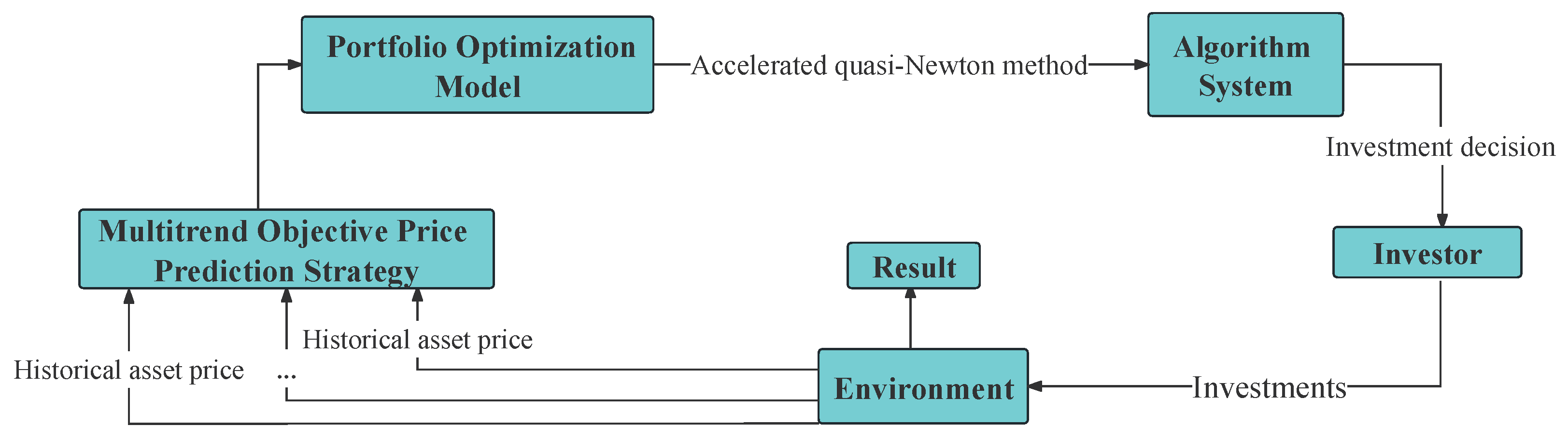
The flowchart of MTO-AQNM is shown in Figure 1. It first gathers historical asset prices. Then it wraps them into a multi-trend objective. In the next step, it uses an accelerated quasi-Newton algorithm to obtain the optimized portfolio. This information is then fed back to the investors for their references.

Figure 1. Flowchart of the whole MTO-AQNM strategy.

4. Experimental Results

We wanted to demonstrate the effectiveness of our model and algorithm using experimental metrics in financial markets where there was asymmetry in all aspects, and we conducted experiments on six benchmark data sets from diverse financial circumstances: NYSE(N) [32], FTSE100 [37], Dowjones [37], HS300 [23], NAS100 [37], and FF32 (http://mba.tuck.dartmouth.edu/pages/faculty/ken.french/data_library.html, accessed on 3 June 2023). Their profiles are given in Table 2. For comparison, we used nine state-of-the-art PO systems: peak price tracking (PPT, [18]), reweighted price relative tracking (RPRT, [38]), kernel-based trend pattern tracking (KTPT, [39]), S1, S2, S3 [40], SSPO [22], adaptive input and composite trend representation (AICTR, [23]), multi-trend conditional value at risk (MT-CVaR, [24]), as well as one trivial system 1/N (equally weighted portfolio, [41]) to test the effectiveness of MTO-AQNM. Moreover, we used multiple indicators to assess the performance of these competitors.

Table 2. Profiles of six benchmark data sets.

Data Set	Region	Time	Periods	Frequency	Assets	Asset Type	Portfolio Type
NYSE(N)	US	1 January 1985∼30 June 2010	6431	Daily	23	Stock	Hybrid Portfolio
FTSE100	UK	11 July 2002∼11 April 2016	717	Weekly	83	Stock	Hybrid Portfolio
Dowjones	US	16 February 1990∼7 April 2016	1363	Weekly	28	Stock	Hybrid Portfolio
HS300	CN	21 January 2016∼16 October 2017	421	Daily	44	Stock	Hybrid Portfolio
NAS100	US	3 November 2004∼11 April 2016	596	Weekly	82	Stock	Hybrid Portfolio
FF32	US	July 1971∼May 2023	623	Monthly	32	Portfolio	Hybrid Portfolio

In the first five data sets, we set the window size $w=5$ for MTO-AQNM, which was the same as other competitors [18,22,23,24,38,40]. In FF32, we set $w=120$ to be consistent with the conventional setting for monthly data in the literature [42,43]. For other parameters of MTO-AQNM, we empirically set $\tau =0.5$, $\gamma =0.005$ and ${\eta }_0=0.8$ for reasonable results. The iteration parameters were set as $Max\_Iter={10}^5$, $Tol={10}^{-4}$ and $\sigma ={10}^7$. The parameters for the quasi-Newton method were set as $\beta =0.2$, $c_1={10}^{-4}$, $c_2=0.9$ and ${\alpha }_0=10$.

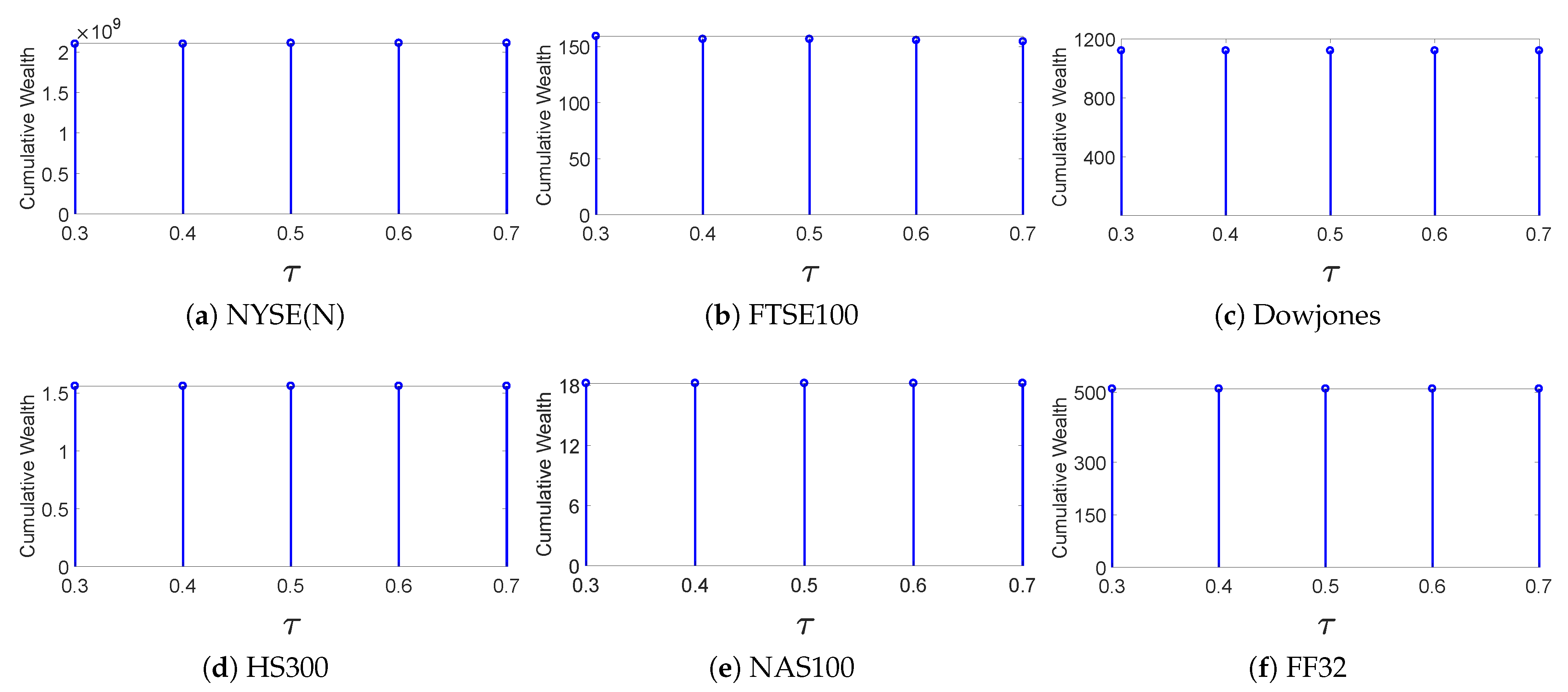
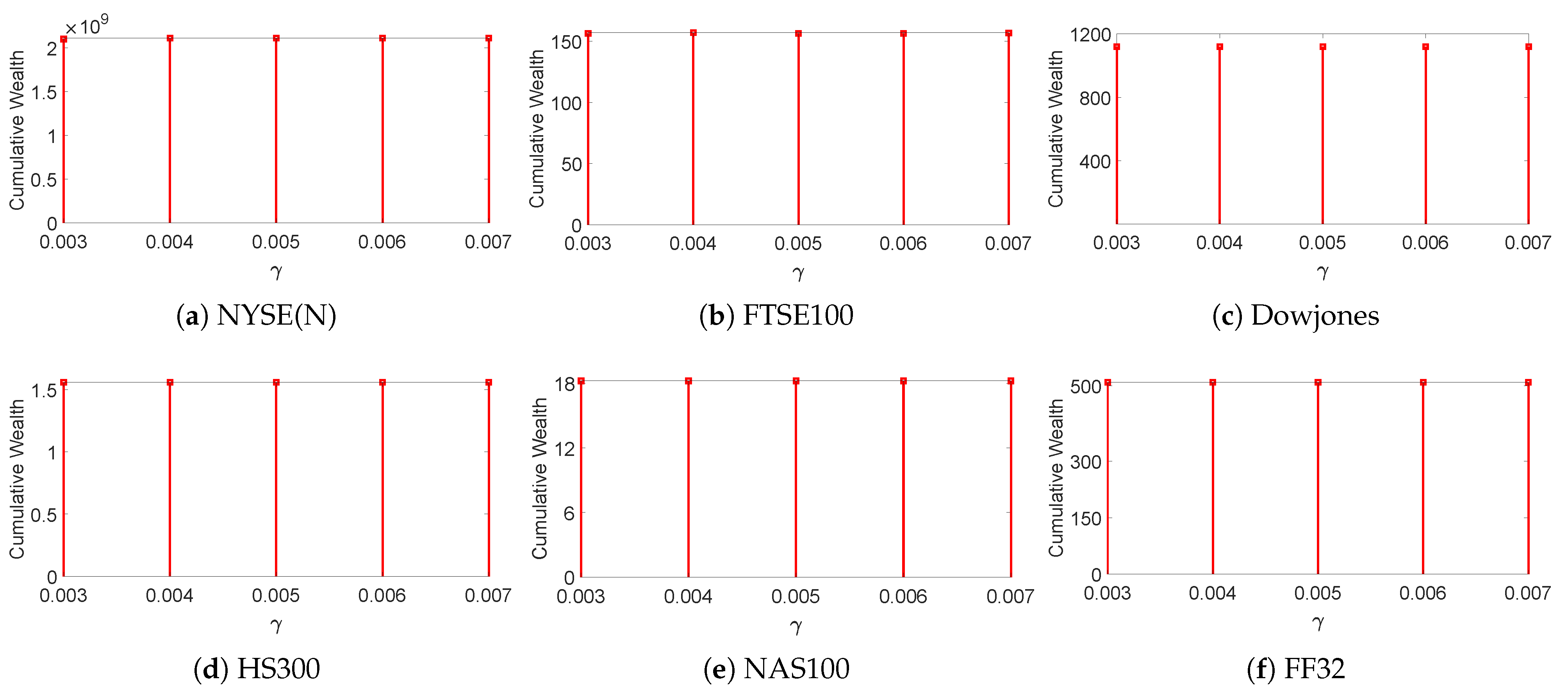
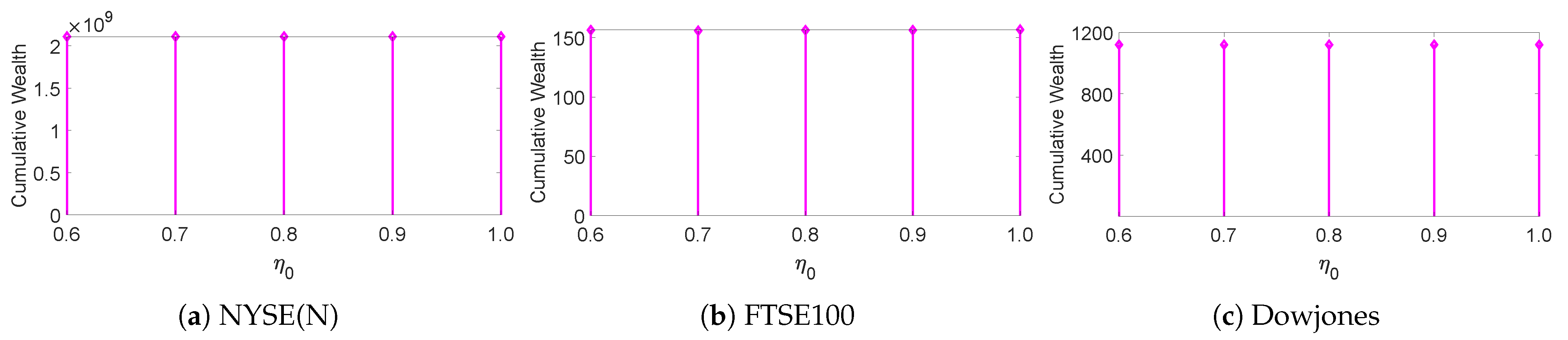
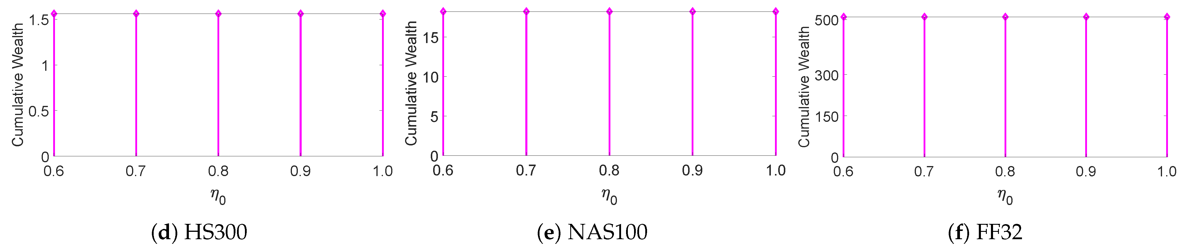
Next, we used ablation experiments to examine whether the key parameters $\tau$, $\gamma$ and ${\eta }_0$ of MTO-AQNM were robust within small changes: $\tau \in (0.3,0.7)$, $\gamma \in (0.003,0.007)$, and ${\eta }_0\in (0.6,1.0)$. We took the final CWs as the evaluating metric, then changed one parameter at a time while fixing the other two as their defaults. The results are shown in Figure 2, Figure 3 and Figure 4, which indicate that MTO-AQNM is robust against small changes of these parameters.

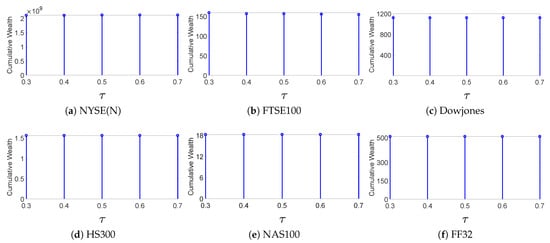
Figure 2. Final cumulative wealths of MTO-AQNM with respect to $\tau$ on six benchmark data sets (fix $\gamma =0.005$ and ${\eta }_0=0.8$).

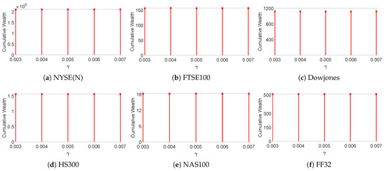
Figure 3. Final cumulative wealths of MTO-AQNM with respect to $\gamma$ on six benchmark data sets (fix $\tau =0.5$ and ${\eta }_0=0.8$).

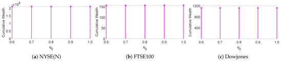
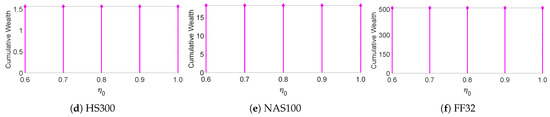
Figure 4. Final cumulative wealths of MTO-AQNM with respect to ${\eta }_0$ on six benchmark data sets (fix $\tau =0.5$ and $\gamma =0.005$).

4.1. Cumulative Wealth and Mean Excess Return

The final cumulative wealth (CW) ${\widehat{S}}_T$ in (3) is a main evaluating metric for a PO system. In addition, the mean excess return (MER, [44]) evaluates the long-term average return of a PO system that surpasses the market strategy:

$$\begin{array}{c}\hfill MER={\overline{r}}_s-{\overline{r}}_m=\frac{1}{T}\sum _{t=1}^T(r_{s,t}-r_{m,t}),\end{array}$$

(39)

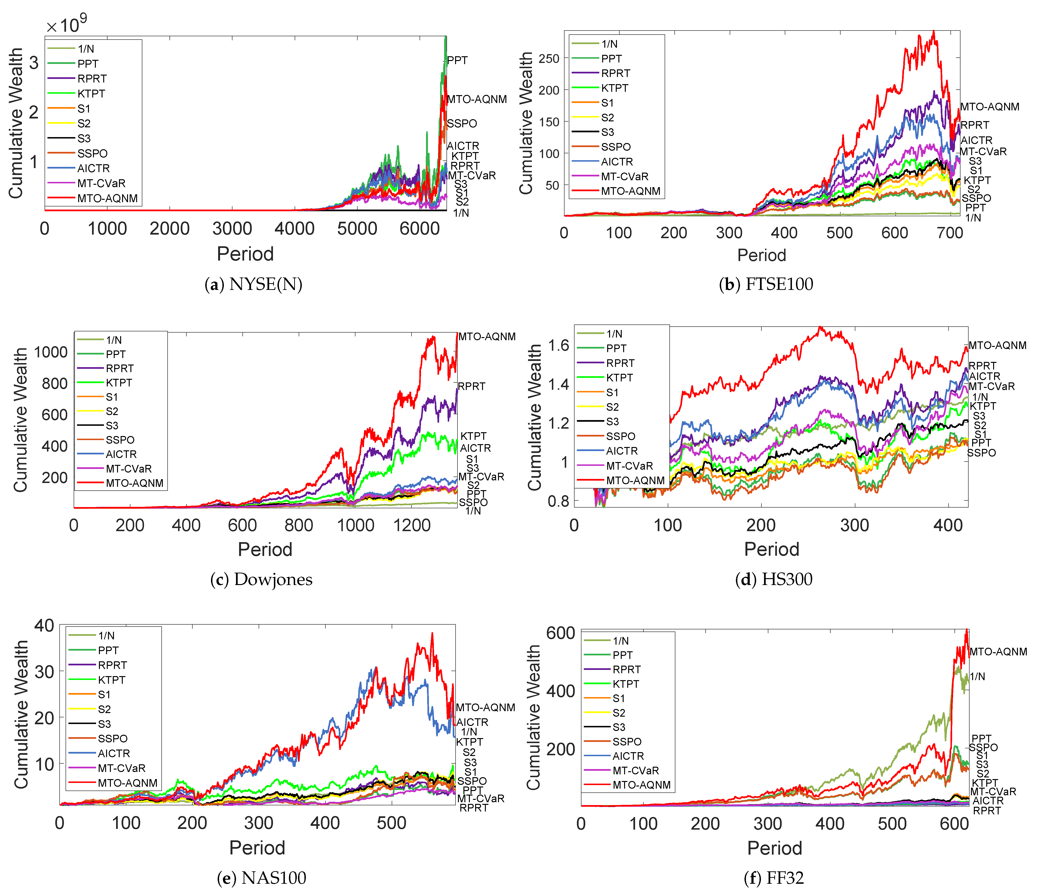
where $r_{s,t}$ and $r_{m,t}$ represent the returns of a PO system and the market strategy on the $t^{\left(th\right)}$ period, respectively. According to [45], the market strategy is computed by the uniform-buy-and-hold strategy. Table 3 shows the CWs and MERs of different PO systems. It indicates that MTO-AQNM outperformed all the other competitors on five out of six data sets. For instance, MTO-AQNM significantly outperformed RPRT (the second place) in CW on Dowjones. Furthermore, only MTO-AQNM ($0.0005$), RPRT (0.0004), AICTR ($0.0003$), and MT-CVaR ($0.0002$) had positive MERs on HS300, among which, MTO-AQNM achieved the highest MER. The MER of MTO-AQNM was significantly higher than those of other competitors on NAS100. In FF32, only MTO-AQNM achieved a positive MER. We also plotted the CWs of different PO systems in Figure 5. The plot of MTO-AQNM remained consistently higher than the other competitors for most of the time. Hence, MTO-AQNM showed effective performance in these two investing metrics.

Table 3. Final cumulative wealths and mean excess returns of portfolio optimization systems on six benchmark data sets.

System	NYSE(N)		FTSE100		Dowjones		HS300		NAS100		FF32
	CW	MER	CW	MER	CW	MER	CW	MER	CW	MER	CW	MER
1/N	$31.55$	$0.0000$	$4.66$	$0.0000$	$33.63$	$-0.0005$	$1.33$	$0.0000$	$6.60$	$-0.0005$	$424.42$	$-0.0005$
PPT	$2.89\times {10}^9$	$0.0036$	$22.28$	$0.0054$	$105.64$	$0.0015$	$1.09$	$-0.0004$	$3.82$	$0.0004$	$149.01$	$-0.0013$
RPRT	$6.25\times {10}^8$	$0.0033$	$133.87$	$0.0074$	$735.63$	$0.0028$	$1.46$	$0.0004$	$3.42$	$0.0001$	$6.28$	$-0.0061$
KTPT	$7.54\times {10}^8$	$0.0033$	$54.22$	$0.0063$	$422.03$	$0.0024$	$1.28$	$0.0000$	$6.44$	$0.0007$	$16.15$	$-0.0052$
S1	$2.37\times {10}^6$	$0.0022$	$54.26$	$0.0061$	$137.79$	$0.0012$	$1.11$	$-0.0004$	$4.36$	$-0.0001$	$32.12$	$-0.0038$
S2	$1.92\times {10}^6$	$0.0022$	$46.50$	$0.0048$	$125.14$	$0.0014$	$1.12$	$-0.0002$	$5.47$	$-0.0011$	$26.58$	$-0.0041$
S3	$2.53\times {10}^6$	$0.0022$	$57.87$	$0.0060$	$135.92$	$0.0016$	$1.20$	$-0.0005$	$4.99$	$0.0003$	$27.08$	$-0.0039$
SSPO	$1.62\times {10}^9$	$0.0035$	$23.94$	$0.0056$	$101.91$	$0.0015$	$1.08$	$-0.0004$	$4.32$	$0.0006$	$130.21$	$-0.0016$
AICTR	$7.66\times {10}^8$	$0.0033$	$89.74$	$0.0070$	$178.84$	$0.0018$	$1.42$	$0.0003$	$15.68$	$0.0026$	$7.88$	$-0.0059$
MT-CVaR	$2.59\times {10}^8$	$0.0031$	$86.96$	$0.0070$	$135.49$	$0.0015$	$1.35$	$0.0002$	$3.75$	$-0.0010$	$12.45$	$-0.0052$
MTO-AQNM	$2.11\times {10}^9$	$0.0034$	$\mathbf{156.22}$	$\mathbf{0.0075}$	$\mathbf{1119.73}$	$\mathbf{0.0031}$	$\mathbf{1.56}$	$\mathbf{0.0005}$	$\mathbf{18.23}$	$\mathbf{0.0029}$	$\mathbf{509.83}$	$\mathbf{0.0010}$

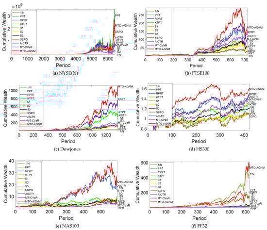
Figure 5. Cumulative wealth plots of portfolio optimization systems on six benchmark data sets.

The Wilcoxon signed-rank test is used to determine whether there is a significant difference between two related or paired samples. In PO, it can be used to compare the performance of portfolios generated by two different methods. To test whether the investment performance of MTO-AQNM is similar to that of competitors, we conducted the Wilcoxon signed-rank test on the CWs between MTO-AQNM and others. Specifically, we computed the CW $S_{s,t}$ for some PO method s at time t, resulting in T samples of $S_{s,t}$ in a data set with T trading periods. Each benchmark data set in this paper had more than 400 trading periods, which is sufficient for statistical tests. The results in Table 4 show that MTO-AQNM differed from each competitor in terms of investment performance, with a confidence level greater than 95% (with all p-values close to 0), suggesting that MTO-AQNM differs significantly from all other competitors in terms of CWs. There is another statistical test for the investing returns in Section 4.2.

Table 4. The p-values of Wilcoxon tests for CWs between MTO-AQNM and other portfolio optimization systems on six benchmark data sets.

System	NYSE(N)	FTSE100	Dowjones	HS300	NAS100	FF32
MTO-AQNM vs. 1/N	$0.0000$	$0.0000$	$0.0000$	$0.0000$	$0.0000$	$0.0000$
MTO-AQNM vs. PPT	$0.0000$	$0.0000$	$0.0000$	$0.0000$	$0.0000$	$0.0000$
MTO-AQNM vs. RPRT	$0.0000$	$0.0000$	$0.0000$	$0.0000$	$0.0000$	$0.0000$
MTO-AQNM vs. KTPT	$0.0000$	$0.0000$	$0.0000$	$0.0000$	$0.0000$	$0.0000$
MTO-AQNM vs. S1	$0.0000$	$0.0000$	$0.0000$	$0.0000$	$0.0000$	$0.0000$
MTO-AQNM vs. S2	$0.0000$	$0.0000$	$0.0000$	$0.0000$	$0.0000$	$0.0000$
MTO-AQNM vs. S3	$0.0000$	$0.0000$	$0.0000$	$0.0000$	$0.0000$	$0.0000$
MTO-AQNM vs. SSPO	$0.0000$	$0.0000$	$0.0000$	$0.0000$	$0.0000$	$0.0000$
MTO-AQNM vs. AICTR	$0.0000$	$0.0000$	$0.0000$	$0.0000$	$0.0000$	$0.0000$
MTO-AQNM vs. MT-CVaR	$0.0000$	$0.0000$	$0.0000$	$0.0000$	$0.0000$	$0.0000$

4.2. The $\alpha$ Factor

The $\alpha$ factor is derived from the capital asset pricing model (CAPM [46]). It represents the pure excess return that excludes market volatility [47]:

$$\begin{array}{cc}\hfill & \mathbb{E}\left(r_s\right)=\alpha +\beta \mathbb{E}\left(r_m\right),\hfill \\ \hfill & \widehat{\beta }=\frac{\widehat{cov}(r_s,r_m)}{{\widehat{\sigma }}^2\left(r_m\right)},\widehat{\alpha }={\overline{r}}_s-\widehat{\beta }{\overline{r}}_m,\hfill \end{array}$$

(40)

where $\widehat{\sigma }$ and $\widehat{cov}$ represent the sample standard deviation (STD) and the covariance during T trading periods, respectively. Table 5 shows the $\alpha$ factors of different PO methods. MTO-AQNM performed better than all the competitors on most data sets, while slightly worse than PPT or 1/N on NYSE(N) or FF32, respectively. Specifically, only MTO-AQNM ($0.0003$), RPRT (0.0001), and AICTR ($0.0001$) achieved positive $\alpha$ factors on HS300. In addition, only MTO-AQNM (0.0021), PPT (0.0004), KTPT (0.0013), S2 (0.0001), SSPO (0.0005), and AICTR (0.0019) achieved positive $\alpha$ factors on NAS100. Furthermore, MTO-AQNM achieved the highest $\alpha$ factors on both data sets. Moreover, whether $\widehat{\alpha }$ was significantly larger than 0 could be tested by a left-tailed t-test in the regression model (40), in order to demonstrate that inherent excess returns were not due to luck. According to the results in Table 5, the confidence level of MTO-AQNM was significantly higher than that of other experimental indicators in multiple markets. For example, in the FTSE100, the confidence level of MTO-AQNM reached 99.44%, far exceeding other systems. In the Dowjones, the confidence level of MTO-AQNM was 99.93%, again showing outstanding performance. These results indicate that the performance of MTO-AQNM in different markets has higher confidence, making it more stable and reliable.

Table 5. The $\alpha$ factors (with p-values of t-tests) of portfolio optimization systems on six benchmark data sets.

System	NYSE(N)		FTSE100		Dowjones		HS300		NAS100		FF32
	$\mathit{\alpha }$	$\mathit{p}$-Value	$\mathit{\alpha }$	$\mathit{p}$-Value	$\mathit{\alpha }$	$\mathit{p}$-Value	$\mathit{\alpha }$	$\mathit{p}$-Value	$\mathit{\alpha }$	$\mathit{p}$-Value	$\mathit{\alpha }$	$\mathit{p}$-Value
1/N	$0.0000$	$0.0314$	$0.0000$	$0.4058$	$0.0010$	$0.0080$	$0.0000$	$0.6273$	$-0.0002$	$0.6975$	$0.0009$	$0.3782$
PPT	$0.0035$	$0.0000$	$0.0037$	$0.0896$	$0.0020$	$0.0536$	$-0.0005$	$0.7465$	$0.0004$	$0.4312$	$-0.0019$	$0.8962$
RPRT	$0.0032$	$0.0000$	$0.0064$	$0.0103$	$0.0036$	$0.0019$	$0.0001$	$0.4364$	$-0.0002$	$0.5396$	$-0.0074$	$1.0000$
KTPT	$0.0032$	$0.0000$	$0.0051$	$0.0301$	$0.0031$	$0.0061$	$0.0000$	$0.5562$	$0.0013$	$0.3035$	$-0.0037$	$0.9877$
S1	$0.0021$	$0.0000$	$0.0046$	$0.0349$	$0.0020$	$0.0241$	$-0.0005$	$0.9060$	$-0.0003$	$0.5707$	$-0.0049$	$0.9998$
S2	$0.0021$	$0.0000$	$0.0045$	$0.0413$	$0.0020$	$0.0288$	$-0.0004$	$0.8596$	$0.0001$	$0.4777$	$-0.0052$	$0.9999$
S3	$0.0022$	$0.0000$	$0.0047$	$0.0322$	$0.0020$	$0.0251$	$-0.0003$	$0.7913$	$-0.0001$	$0.5152$	$-0.0051$	$0.9997$
SSPO	$0.0034$	$0.0000$	$0.0040$	$0.0799$	$0.0020$	$0.0552$	$-0.0005$	$0.7620$	$0.0005$	$0.4173$	$-0.0020$	$0.9221$
AICTR	$0.0032$	$0.0000$	$0.0055$	$0.0167$	$0.0025$	$0.0208$	$0.0001$	$0.4638$	$0.0019$	$0.1876$	$-0.0068$	$1.0000$
MT-CVaR	$0.0031$	$0.0000$	$0.0054$	$0.0184$	$0.0022$	$0.0327$	$-0.0002$	$0.5113$	$-0.0006$	$0.6764$	$-0.0062$	$1.0000$
MTO-AQNM	$0.0034$	$0.0000$	$\mathbf{0.0065}$	$0.0056$	$\mathbf{0.0040}$	$0.0007$	$\mathbf{0.0003}$	$0.3373$	$\mathbf{0.0021}$	$0.1706$	$-0.0020$	$0.5378$

The $\widehat{\beta }$ factor is a core part of the CAPM and is used to calculate the expected return and risk of an asset. The $\widehat{\beta }$ factor reflects the volatility of a portfolio relative to a market benchmark. It reflects the relationship between a stock or portfolio and the systematic risk of the market. When $\widehat{\beta }=1$, it indicates that the asset price fluctuates in synchronization with the market; when $\widehat{\beta }<1$, it indicates that the asset price fluctuates less than the market, and when $\widehat{\beta }>1$, it indicates that the asset price fluctuates more than the market. Table 6 shows that the MTO-AQNM system is more stable compared to other systems.

Table 6. The $\beta$ factors of portfolio optimization systems on six benchmark data sets.

System	NYSE(N)	FTSE100	Dowjones	HS300	NAS100	FF32
1/N	$1.0164$	$1.0034$	$0.5598$	$0.9908$	$0.9245$	$0.9474$
PPT	$1.1210$	$1.6813$	$0.8419$	$1.1204$	$0.9914$	$1.1088$
RPRT	$1.1518$	$1.5201$	$0.7674$	$1.2841$	$1.0737$	$1.1096$
KTPT	$1.1347$	$1.4942$	$0.7945$	$1.0332$	$1.0620$	$0.8630$
S1	$1.1350$	$1.6217$	$0.7798$	$1.1180$	$1.0471$	$1.1011$
S2	$1.1040$	$1.5744$	$0.7655$	$1.1268$	$1.0771$	$1.0804$
S3	$1.1285$	$1.6135$	$0.7841$	$1.1111$	$1.0378$	$1.0950$
SSPO	$1.1161$	$1.6471$	$0.8387$	$1.1143$	$1.0203$	$1.0352$
AICTR	$1.1710$	$1.6088$	$0.7825$	$1.2564$	$1.1589$	$1.0947$
MT-CVaR	$1.1505$	$1.6468$	$0.8001$	$1.2126$	$0.9038$	$1.0899$
MTO-AQNM	$1.0375$	$1.2228$	$0.8469$	$1.2540$	$1.0956$	$1.0968$

4.3. Sharpe Ratio and Information Ratio

In both theoretical and practical portfolio management, it is consistently observed that higher returns tend to be associated with higher risks. The Sharpe ratio (SR [48]) serves as a conventional metric for evaluating the risk-adjusted returns and assessing the risk control efficacy of PO systems. It is defined as

$$\begin{array}{c}\hfill SR=\frac{{\overline{r}}_s-r_f}{\widehat{\sigma }\left(r_s\right)},\end{array}$$

(41)

where $r_f$ corresponds to the risk-free return. Since the risk-free asset was not considered in this paper, $r_f$ was set to 0.

Another similar metric in this context is the information ratio (IR, [49]), but it directly calculates the returns and risks relative to the market strategy:

$$\begin{array}{c}\hfill IR=\frac{{\overline{r}}_s-{\overline{r}}_m}{\widehat{\sigma }(r_s-r_m)}.\end{array}$$

(42)

Table 7 shows the SRs and IRs of different PO systems. MTO-AQNM achieved the highest SRs and IRs in most cases. According to [41], 1/N has a natural risk-control inclination and, thus, achieves high SRs. Nevertheless, MTO-AQNM still outperformed 1/N in 9 out of 12 cases. Hence, MTO-AQNM is also competitive in regard to risk control.

Table 7. Sharpe ratios and information ratios of portfolio optimization systems on six benchmark data sets.

System	NYSE(N)		FTSE100		Dowjones		HS300		NAS100		FF32
	SR	IR	SR	IR	SR	IR	SR	IR	SR	IR	SR	IR
1/N	$0.0506$	$0.0255$	$0.0933$	$0.0100$	$0.1112$	$-0.0256$	$0.0734$	$-0.0275$	$0.1221$	$-0.0581$	$0.2213$	$-0.0690$
PPT	$0.1087$	$0.1008$	$0.0915$	$0.0711$	$0.0894$	$0.0320$	$0.0246$	$-0.0255$	$0.0673$	$0.0066$	$0.1557$	$-0.0359$
RPRT	$0.1046$	$0.0967$	$0.1210$	$0.1023$	$0.1173$	$0.0605$	$0.0550$	$0.0228$	$0.0648$	$0.0014$	$0.0775$	$-0.1539$
KTPT	$0.1067$	$0.0988$	$0.1073$	$0.0864$	$0.1093$	$0.0524$	$0.0424$	$0.0007$	$0.0709$	$0.0114$	$0.1048$	$-0.1275$
S1	$0.0903$	$0.0807$	$0.1079$	$0.0883$	$0.1012$	$0.0327$	$0.0244$	$-0.0516$	$0.0731$	$-0.0030$	$0.1174$	$-0.1109$
S2	$0.0782$	$0.0678$	$0.0868$	$0.0646$	$0.0931$	$0.0317$	$0.0293$	$-0.0128$	$0.0476$	$-0.0213$	$0.1112$	$-0.1128$
S3	$0.0867$	$0.0767$	$0.1062$	$0.0863$	$0.1059$	$0.0401$	$0.0166$	$-0.0494$	$0.0799$	$0.0072$	$0.1131$	$-0.1088$
SSPO	$0.1060$	$0.0979$	$0.0929$	$0.0727$	$0.0887$	$0.0314$	$0.0231$	$-0.0275$	$0.0704$	$0.0100$	$0.1542$	$-0.0466$
AICTR	$0.1056$	$0.0979$	$0.1179$	$0.0998$	$0.0978$	$0.0386$	$0.0555$	$0.0181$	$0.1042$	$0.0486$	$0.0827$	$-0.1509$
MT-CVaR	$0.1020$	$0.0939$	$0.1168$	$0.0989$	$0.0947$	$0.0342$	$0.0476$	$0.0106$	$0.0751$	$-0.0314$	$0.0937$	$-0.1358$
MTO-AQNM	$\mathbf{0.1125}$	$\mathbf{0.1050}$	$\mathbf{0.1290}$	$\mathbf{0.1092}$	$\mathbf{0.1243}$	$\mathbf{0.0666}$	$0.0657$	$\mathbf{0.0347}$	$0.1074$	$\mathbf{0.0538}$	$0.1754$	$\mathbf{0.0223}$

4.4. Treynor Ratio

The Treynor ratio (TR, [50]) is the ratio of the excess return to the $\beta$ factor in (40). It measures the systematic-risk-adjusted excess return for a PO system, since the $\beta$ factor is a metric for the systematic risk. TR can be calculated as follows:

$$\begin{array}{c}\hfill TR=\frac{{\overline{r}}_s-r_f}{\widehat{\beta }}.\end{array}$$

(43)

Table 8 presents the TRs for different PO systems. MTO-AQNM achieved the best TRs across most data sets, except on NYSE(N) or FF32, where it was slightly worse than PPT or 1/N, respectively. This indicates that MTO-AQNM is competitive in systematic risk control.

Table 8. Treynor ratios of portfolio optimization systems on six benchmark data sets.

System	NYSE(N)	FTSE100	Dowjones	HS300	NAS100	FF32
1/N	$0.0006$	$0.0025$	$0.0052$	$0.0007$	$0.0039$	$0.0116$
PPT	$0.0036$	$0.0047$	$0.0059$	$0.0003$	$0.0045$	$0.0097$
RPRT	$0.0033$	$0.0068$	$0.0082$	$0.0009$	$0.0039$	$0.0049$
KTPT	$0.0034$	$0.0059$	$0.0074$	$0.0007$	$0.0047$	$0.0073$
S1	$0.0024$	$0.0053$	$0.0060$	$0.0003$	$0.0038$	$0.0071$
S2	$0.0024$	$0.0046$	$0.0064$	$0.0005$	$0.0027$	$0.0069$
S3	$0.0024$	$0.0053$	$0.0064$	$0.0002$	$0.0042$	$0.0069$
SSPO	$0.0036$	$0.0048$	$0.0059$	$0.0003$	$0.0046$	$0.0096$
AICTR	$0.0033$	$0.0059$	$0.0067$	$0.0008$	$0.0057$	$0.0052$
MT-CVaR	$0.0032$	$0.0057$	$0.0062$	$0.0007$	$0.0034$	$0.0059$
MTO-AQNM	$0.0035$	$\mathbf{0.0070}$	$\mathbf{0.0088}$	$\mathbf{0.0010}$	$\mathbf{0.0058}$	$0.0114$

4.5. Sortino Ratio

The Sortino ratio [51] is a metric used in the field of finance and investment to measure the risk-adjusted return of an investment. It is an improvement on the Sharpe ratio, specifically taking into account downside risk rather than total volatility. The Sortino ratio can be calculated as follows:

$$\begin{array}{c}\hfill SortinoRatio=\frac{{\overline{r}}_s-r_f}{{\sigma }_d},{\sigma }_d=\sqrt{{\displaystyle \frac{1}{T}\sum _{t=1}^T{\left({\overline{r}}_{s,t}-r_{f,t}\right)}^2}},\end{array}$$

(44)

where ${\sigma }_d$ is the downside standard deviation. Table 9 presents the Sortino ratios for different PO systems. MTO-AQNM achieved the best Sortino ratios on most of the data sets, with only a slight inferiority of 1/N on FF32. This suggests that MTO-AQNM has more effective risk management under downside market conditions.

Table 9. Sortino ratios of portfolio optimization systems on six benchmark data sets.

System	NYSE(N)	FTSE100	Dowjones	HS300	NAS100	FF32
1/N	$0.0790$	$0.1555$	$0.2025$	$0.0917$	$0.1882$	$0.3795$
PPT	$0.1957$	$0.1760$	$0.1560$	$0.0309$	$0.1122$	$0.2755$
RPRT	$0.1870$	$0.2333$	$0.2068$	$0.0864$	$0.1072$	$0.1308$
KTPT	$0.1935$	$0.2051$	$0.1954$	$0.0647$	$0.1399$	$0.1706$
S1	$0.1636$	$0.2084$	$0.1773$	$0.0344$	$0.1196$	$0.2044$
S2	$0.1401$	$0.1636$	$0.1576$	$0.0471$	$0.0783$	$0.1939$
S3	$0.1573$	$0.2048$	$0.1882$	$0.0245$	$0.1321$	$0.1991$
SSPO	$0.1923$	$0.1786$	$0.1557$	$0.0286$	$0.1181$	$0.2760$
AICTR	$0.1893$	$0.2163$	$0.1709$	$0.0805$	$0.1834$	$0.1361$
MT-CVaR	$0.1811$	$0.2169$	$0.1657$	$0.0714$	$0.1116$	$0.1598$
MTO-AQNM	$\mathbf{0.2092}$	$\mathbf{0.2416}$	$\mathbf{0.2226}$	$\mathbf{0.1017}$	$\mathbf{0.1933}$	$0.3298$

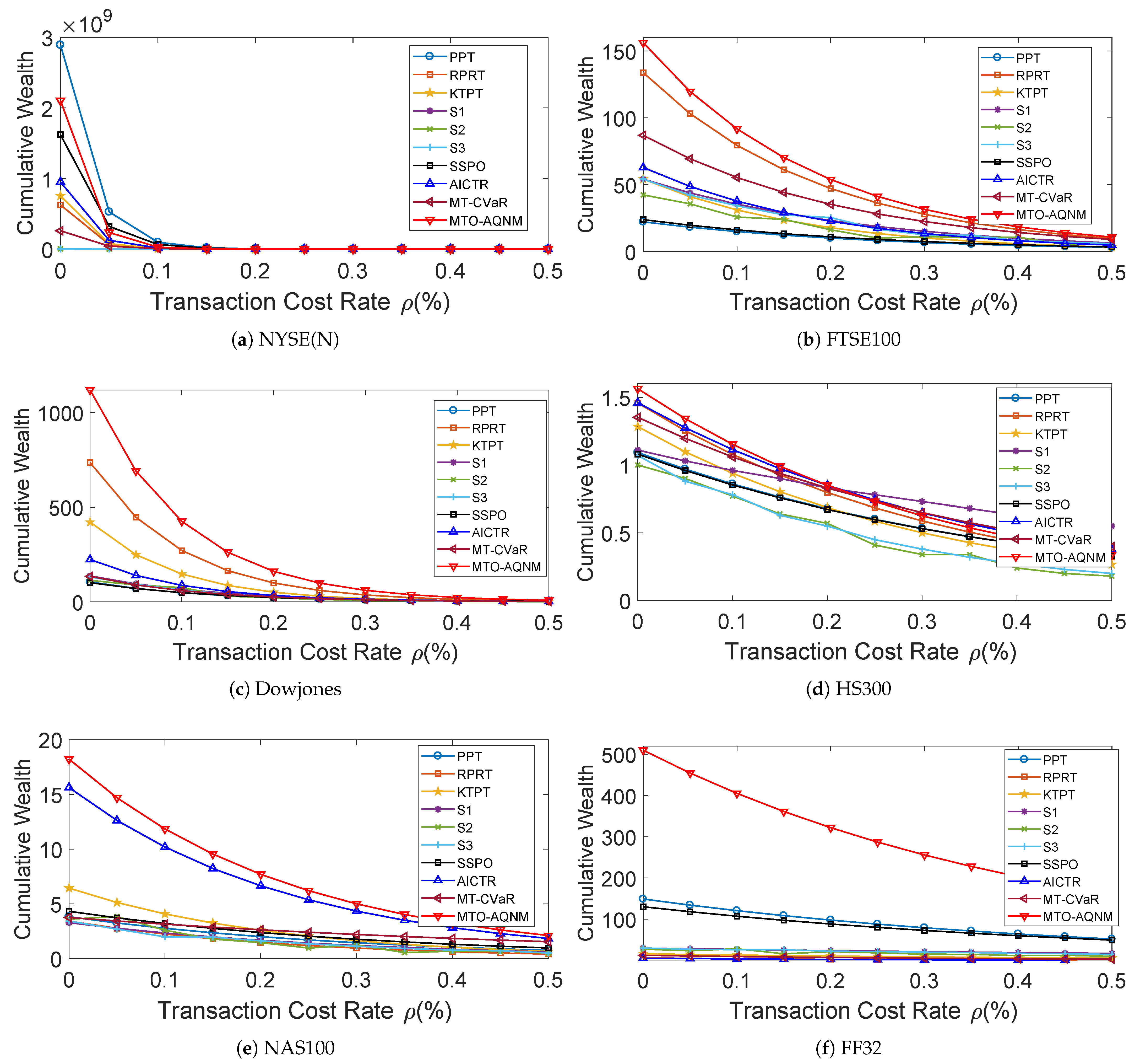
4.6. Transaction Cost

To assess the influence of transaction costs on the performance of the PO systems, we employed a proportional transaction cost model [2,14,52] to compute CWs associated with transaction costs:

$$\begin{array}{cc}\hfill S_T^{\rho }& =S_0\prod _{t=1}^T[\left({\widehat{\mathbf{b}}}_t^{\top }{\mathbf{x}}_t\right)·(1-\frac{\rho }{2}\sum _{i=1}^d|{\widehat{\mathbf{b}}}_t^{\left(i\right)}-{\tilde{\mathbf{b}}}_{t-1}^{\left(i\right)}\left|\right)],\hfill \end{array}$$

(45)

$$\begin{array}{cc}\hfill {\tilde{\mathbf{b}}}_{t-1}^{\left(i\right)}& =\frac{{\widehat{\mathbf{b}}}_{t-1}^{\left(i\right)}{\mathbf{x}}_{t-1}^{\left(i\right)}}{{\widehat{\mathbf{b}}}_{t-1}^{\top }{\mathbf{x}}_{t-1}},\hfill \end{array}$$

(46)

where ${\tilde{\mathbf{b}}}_{t-1}^{\left(i\right)}$ denotes the updated portfolio of the ith asset at the end of period $(t-1)$, while $\rho$ represents the bidirectional transaction cost rate. If the cost rates for buying and selling were equal, then transitioning from the evolved portfolio ${\tilde{\mathbf{b}}}_{t-1}$ to the subsequent portfolio ${\widehat{\mathbf{b}}}_t$ incurred a proportional transaction cost of $\frac{\rho }{2}{\sum }_{i=1}^d|{\widehat{\mathbf{b}}}_t^{\left(i\right)}-{\tilde{\mathbf{b}}}_{t-1}^{\left(i\right)}|$. By varying $\rho$ from 0 to $0.5\%$, the final CWs of different PO systems are depicted in Figure 6. In general, MTO-AQNM performed well, with moderate-to-low transaction cost rates. If a fund was operating with large enough capital, $\rho$ could be negotiated to be very small (e.g., ≤0.05%). Hence MTO-AQNM is able to withstand a certain level of transaction cost.

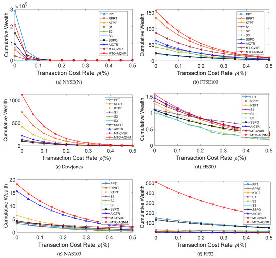
Figure 6. Final cumulative wealths of portfolio optimization systems with respect to transaction cost rate $\rho$ on six benchmark data sets.

4.7. Accelerated Quasi-Newton Method vs. First-Order Method

For this part, we examined whether the proposed AQNM runs faster than an ordinary first-order subgradient descent method. The computing machine was an ordinary personal computer with an Intel Core i7-10700 2.90 GHz CPU and an 8 GB 2933 MHz DDR4 RAM. Table 10 shows the average running times and iterations per trading period for both algorithms with the same parameters. It shows that AQNM greatly reduces the number of iterations and running times compared with the first-order method. In fact, the first-order method cannot converge until reaching the maximum iterations, while AQNM can finish computation in only a few seconds. This indicates that AQNM is necessary and efficient in solving the proposed PO model.

Table 10. Average running times (in seconds) and iterations per trading period for accelerated quasi-Newton method and first-order method.

Algorithm	NYSE(N)		FTSE100		Dowjones		HS300		NAS100		FF32
	Time	Iter.	Time	Iter.	Time	Iter.	Time	Iter.	Time	Iter.	Time	Iter.
First-order	$1145.4971$	100,000	$141.5923$	100,000	$246.2983$	100,000	$75.4959$	100,000	$117.6703$	100,000	$112.4363$	100,000
AQNM	$\mathbf{8.6836}$	$\mathbf{9.7988}$	$\mathbf{1.2089}$	$\mathbf{7.6360}$	$\mathbf{1.0718}$	$\mathbf{7.8921}$	$\mathbf{0.3761}$	$\mathbf{7.7553}$	$\mathbf{0.9090}$	$\mathbf{7.3993}$	$\mathbf{2.2292}$	$\mathbf{7.2857}$

5. Conclusions

This paper proposes a multi-trend objective and accelerated quasi-Newton method (MTO-AQNM) for portfolio optimization. Some existing state-of-the-art portfolio optimization systems mainly focus on trend-reversing and multi-trend representation. MTO-AQNM combines four trend-reversing representations into one objective function, which is more adaptive to the fluctuations of financial markets. To solve this model, MTO-AQNM uses the BFGS method with the Wolfe conditions to reduce computational complexity and improve convergence speed.

Extensive experiments on six data sets showed that MTO-AQNM is effective in portfolio optimization. It outperformed nine state-of-the-art competitors in most cases regarding cumulative wealth, mean excess return, and $\alpha$ factor, showing good ability for gaining returns. It also achieved the highest Sharpe ratios, information ratios and Treynor ratios in most cases, showing good risk control ability. As for practical issues, MTO-AQNM can withstand a certain level of transaction costs and it runs fast. Future works may fall into developing new multi-trend objective models and corresponding efficient solving algorithms.

References

- Markowitz, H.M. Portfolio Selection. J. Financ. 1952, 7, 77–91. [Google Scholar]
- Lai, Z.R.; Yang, H. A Survey on Gaps between Mean-variance Approach and Exponential Growth Rate Approach for Portfolio Optimization. ACM Comput. Surv. 2023, 55, 1–36. [Google Scholar] [CrossRef]
- Kalina, B.; Lee, J.H.; Na, K.T. Enhancing Portfolio Performance through Financial Time-Series Decomposition-Based Variational Encoder-Decoder Data Augmentation. Symmetry 2024, 16, 283. [Google Scholar] [CrossRef]
- Dreżewski, R.; Doroz, K. An Agent-Based Co-Evolutionary Multi-Objective Algorithm for Portfolio Optimization. Symmetry 2017, 9, 168. [Google Scholar] [CrossRef]
- Wu, C.; Yang, L.; Zhang, C. Uncertain Stochastic Optimal Control with Jump and Its Application in a Portfolio Game. Symmetry 2022, 14, 1885. [Google Scholar] [CrossRef]
- Kelly, J. A new interpretation of information rate. IRE Trans. Inf. Theory 1956, 2, 185–189. [Google Scholar] [CrossRef]
- Ban, G.Y.; Karoui, N.E.; Lim, A.E.B. Machine Learning and Portfolio Optimization. Manag. Sci. 2018, 64, 1136–1154. [Google Scholar] [CrossRef]
- Ledoit, O.; Wolf, M. Nonlinear Shrinkage of the Covariance Matrix for Portfolio Selection: Markowitz Meets Goldilocks. Rev. Financ. Stud. 2017, 30, 4349–4388. [Google Scholar] [CrossRef]
- Li, D.; Ng, W.L. Optimal Dynamic Portfolio Selection: Multiperiod Mean-Variance Formulation. Math. Financ. 2000, 10, 387–406. [Google Scholar] [CrossRef]
- Kolm, P.N.; Tütüncü, R.; Fabozzi, F.J. 60 Years of portfolio optimization: Practical challenges and current trends. Eur. J. Oper. Res. 2014, 234, 356–371. [Google Scholar] [CrossRef]
- Kahneman, D.; Tversky, A. Prospect Theory: An Analysis of Decision under Risk. Econometrica 1979, 47, 263–292. [Google Scholar] [CrossRef]
- Shiller, R.J. From Efficient Markets Theory to Behavioral Finance. J. Econ. Perspect. 2003, 17, 83–104. [Google Scholar] [CrossRef]
- Shiller, R.J. Irrational Exuberance; Wiley: New York, NY, USA, 2000. [Google Scholar]
- Li, B.; Hoi, S.C.H.; Sahoo, D.; Liu, Z.Y. Moving average reversion strategy for on-line portfolio selection. Artif. Intell. 2015, 222, 104–123. [Google Scholar] [CrossRef]
- Huang, D.; Zhou, J.; Li, B.; Hoi, S.C.H.; Zhou, S. Robust Median Reversion Strategy for Online Portfolio Selection. IEEE Trans. Knowl. Data Eng. 2016, 28, 2480–2493. [Google Scholar] [CrossRef]
- Liu, Z.; Dong, X.; Xue, J.; Li, H.; Chen, Y. Adaptive neural control for a class of pure-feedback nonlinear systems via dynamic surface technique. IEEE Trans. Neural Netw. Learn. Syst. 2015, 27, 1969–1975. [Google Scholar] [CrossRef] [PubMed]
- Agarwal, A.; Hazan, E.; Kale, S.; Schapire, R.E. Algorithms for portfolio management based on the Newton method. In Proceedings of the International Conference on Machine Learning (ICML), Pittsburgh, PA, USA, 25–29 June 2006. [Google Scholar]
- Lai, Z.R.; Dai, D.Q.; Ren, C.X.; Huang, K.K. A Peak Price Tracking based Learning System for Portfolio Selection. IEEE Trans. Neural Netw. Learn. Syst. 2018, 29, 2823–2832. [Google Scholar] [CrossRef] [PubMed]
- Helmbold, D.P.; Schapire, R.E.; Singer, Y.; Warmuth, M.K. On-line portfolio selection using multiplicative updates. Math. Financ. 1998, 8, 325–347. [Google Scholar] [CrossRef]
- Györfi, L.; Udina, F.; Walk, H. Nonparametric nearest neighbor based empirical portfolio selection strategies. Stat. Decis. 2008, 26, 145–157. [Google Scholar] [CrossRef]
- Li, B.; Zhao, P.; Hoi, S.C.H.; Gopalkrishnan, V. PAMR: Passive aggressive mean reversion strategy for portfolio selection. Mach. Learn. 2012, 87, 221–258. [Google Scholar] [CrossRef]
- Lai, Z.R.; Yang, P.Y.; Fang, L.; Wu, X. Short-term Sparse Portfolio Optimization Based on Alternating Direction Method of Multipliers. J. Mach. Learn. Res. 2018, 19, 1–28. [Google Scholar]
- Lai, Z.R.; Dai, D.Q.; Ren, C.X.; Huang, K.K. Radial basis functions with adaptive input and composite trend representation for portfolio selection. IEEE Trans. Neural Netw. Learn. Syst. 2018, 29, 6214–6226. [Google Scholar] [CrossRef] [PubMed]
- Lai, Z.R.; Li, C.; Wu, X.; Guan, Q.; Fang, L. Multitrend Conditional Value at Risk for Portfolio Optimization. IEEE Trans. Neural Netw. Learn. Syst. 2024, 35, 1545–1558. [Google Scholar] [CrossRef] [PubMed]
- Wang, H.; Liu, J.; Liu, Y. A New Self-Scaling Memoryless Quasi-Newton Update for Portfolio Optimization. Comput. Optim. Appl. 2023, 84, 725–745. [Google Scholar]
- Kumar, K.; Ghosh, D.; Upadhayay, A.; Yao, J.; Zhao, X. Quasi-Newton Methods for Multiobjective Optimization Problems: A Systematic Review. Appl. Set-Valued Anal. Optim. 2023, 5, 291–321. [Google Scholar]
- Wright, J.N.S.J. Numerical Optimization; Springer: New York, NY, USA, 2006. [Google Scholar]
- Cover, T.M. Universal Portfolios. Math. Financ. 1991, 1, 1–29. [Google Scholar] [CrossRef]
- Bondt, W.F.M.D.; Thaler, R. Does the Stock Market Overreact? J. Financ. 1985, 40, 793–805. [Google Scholar] [CrossRef]
- Lo, A.W.; MacKinlay, A.C. When Are Contrarian Profits Due to Stock Market Overreaction? Rev. Financ. Stud. 2015, 3, 175–205. [Google Scholar] [CrossRef]
- Borodin, A.; El-Yaniv, R.; Gogan, V. Can We Learn to Beat the Best Stock. J. Artif. Intell. Res. 2004, 21, 579–594. [Google Scholar] [CrossRef]
- Li, B.; Hoi, S.C.H.; Zhao, P.; Gopalkrishnan, V. Confidence Weighted Mean Reversion Strategy for Online Portfolio Selection. ACM Trans. Knowl. Discov. Data 2013, 7, 4. [Google Scholar] [CrossRef]
- Boyd, S.; Vandenberghe, L. Convex Optimization; Cambridge University Press: Cambridge, UK, 2004. [Google Scholar]
- Yuan, Y.; Sun, W. Optimization Theory and Methods; Science Press: Beijing, China, 1999. [Google Scholar]
- Bertsekas, D. Nonlinear Programming; Athena Scientific: Nashua, NH, USA, 1999. [Google Scholar]
- Duchi, J.; Shalev-Shwartz, S.; Singer, Y.; Chandra, T. Efficient projections onto the ℓ1-ball for learning in high dimensions. In Proceedings of the International Conference on Machine Learning (ICML), Helsinki, Finland, 5–9 July 2008. [Google Scholar]
- Bruni, R.; Cesarone, F.; Scozzari, A.; Tardella, F. Real-world datasets for portfolio selection and solutions of some stochastic dominance portfolio models. Data Brief 2016, 8, 858–862. [Google Scholar] [CrossRef]
- Lai, Z.R.; Yang, P.Y.; Fang, L.; Wu, X. Reweighted Price Relative Tracking System for Automatic Portfolio Optimization. IEEE Trans. Syst. Man, Cybern. Syst. 2020, 50, 4349–4361. [Google Scholar] [CrossRef]
- Lai, Z.R.; Yang, P.Y.; Wu, X.; Fang, L. A Kernel-based Trend Pattern Tracking System for Portfolio Optimization. Data Min. Knowl. Discov. 2018, 32, 1708–1734. [Google Scholar] [CrossRef]
- Luo, Z.; Yu, X.; Xiu, N.; Wang, X. Closed-form solutions for short-term sparse portfolio optimization. Optimization 2020, 71, 1937–1953. [Google Scholar] [CrossRef]
- DeMiguel, V.; Garlappi, L.; Uppal, R. Optimal versus Naive Diversification: How Inefficient Is the 1/N Portfolio Strategy? Rev. Financ. Stud. 2009, 22, 1915–1953. [Google Scholar] [CrossRef]
- Goto, S.; Xu, Y. Improving Mean Variance Optimization through Sparse Hedging Restrictions. J. Financ. Quant. Anal. 2015, 50, 1415–1441. [Google Scholar] [CrossRef]
- Ao, M.; Li, Y.; Zheng, X. Approaching Mean-Variance Efficiency for Large Portfolios. Rev. Financ. Stud. 2019, 32, 2890–2919. [Google Scholar] [CrossRef]
- Jegadeesh, N. Evidence of Predictable Behavior of Security Returns. J. Financ. 1990, 45, 881–898. [Google Scholar] [CrossRef]
- Li, B.; Sahoo, D.; Hoi, S.C.H. OLPS: A toolbox for on-line portfolio selection. J. Mach. Learn. Res. 2016, 17, 1242–1246. [Google Scholar]
- Sharpe, W.F. Capital Asset Prices: A Theory of Market Equilibrium under Conditions of Risk. J. Financ. 1964, 19, 425–442. [Google Scholar]
- Lintner, J. The Valuation of Risk Assets and the Selection of Risky Investments in Stock Portfolios and Capital Budgets. Rev. Econ. Stat. 1965, 47, 13–37. [Google Scholar] [CrossRef]
- Sharpe, W.F. Mutual Fund Performance. J. Bus. 1966, 39, 119–138. [Google Scholar] [CrossRef]
- Treynor, J.L.; Black, F. How to Use Security Analysis to Improve Portfolio Selection. J. Bus. 1973, 46, 66–86. [Google Scholar] [CrossRef]
- Treynor, J.L. Towards a Theory of Market Value of Risky Assets. J. Financ. 1965, 20, 415–429. [Google Scholar]
- Sortino, F.A. The Sortino Framework for Constructing Portfolios; Elsevier Science: Amsterdam, The Netherlands, 2009. [Google Scholar]
- Blum, A.; Kalai, A. Universal Portfolios With and Without Transaction Costs. Mach. Learn. 1999, 35, 193–205. [Google Scholar] [CrossRef]
Disclaimer/Publisher’s Note: The statements, opinions and data contained in all publications are solely those of the individual author(s) and contributor(s) and not of MDPI and/or the editor(s). MDPI and/or the editor(s) disclaim responsibility for any injury to people or property resulting from any ideas, methods, instructions or products referred to in the content. |
© 2024 by the authors. Licensee MDPI, Basel, Switzerland. This article is an open access article distributed under the terms and conditions of the Creative Commons Attribution (CC BY) license (https://creativecommons.org/licenses/by/4.0/).