Abstract
The inherent stochasticity of electric operation vehicle (EOV) charging poses challenges to the stability and efficiency of regional power distribution networks. Existing charging behavior decision-making models often prioritize revenue considerations, neglecting the influence of multi-time-span characteristics and the potential irrationality of EOV owners. To address these limitations, this study proposes a comprehensive framework encompassing three aspects. First, operational data are statistically analyzed to reconstruct EOV operation scenarios, establishing a dynamic charging scheme tailored to multi-time-span characteristics. Second, an improved ITCH model is developed using operational equivalent change to incorporate both gains and losses. Third, a WFL framework is employed to integrate the perceptual attenuation of revenue into the ITCH model. Simulation results show that decision-makers (DMs) demonstrate a preference for charging schemes with high equivalent perceived revenues and low time costs. Moreover, when the charging price is doubled, revenue perception attenuation leads decision-makers to postpone their charging behavior. Compared to other models, the equivalent perception intertemporal choice heuristics (EP-ITCH) charging model results in reduced load peaks, valleys, and variances on the grid side. This study highlights the model’s effectiveness and accuracy in optimizing EOV charging infrastructure.
1. Introduction
In recent years, electric vehicles (EVs) have become highly regarded for their characteristics such as “electricity instead of fuel”, environmental cleanliness, low emissions, and high efficiency. However, the increasing penetration rate of EVs brings enormous panoramic situational awareness data, which poses new challenges for power grid planning and scheduling, stability control, and operation [1,2,3,4]. The large-scale integration of EVs will lead to an increase in peak-to-valley differences in electricity demand, affecting the stable operation of networks [5,6,7]. In addition, the chaotic charging behavior of EV owners, which form charging clusters, can result in the irrational allocation of electric power resources. Clusters of electric operation vehicles (EOVs) exhibit characteristics such as greater charging frequencies and charging power compared to conventional EV clusters. They have a more significant impact on the stable operation of power grids, making the study of charging-related issues for EOVs of great significance.
In the research on EV charging schemes, Chen et al. and Wang et al. simulated EV charging schemes using the Monte Carlo method [8,9]. However, due to the lack of modeling based on real operational data, the schemes and the charging strategies still need further validation. H. Al-Alwash et al. considered user preferences in waiting time and charging prices and established a real-time interaction model based on software-defined networking and cloud computing [10]; however, the issue of operational losses for EV owners was neglected. Feng et al. constructed charging schemes by considering both arrival times and left-over battery charge [11]; however, the research failed to organically integrate charging schemes and the value function of charging behaviors.
In terms of modeling charging decisions, Chakraborty A. points out that exponential discounting is widely used in economics to balance alternative scenarios obtained at different time points [12]. However, discounting models are rooted in economic theory and cannot fully explain the psychological principles and cognitive processes that influence intertemporal decision making. Feng et al. introduced the cumulative prospect theory, which considers the heterogeneity of the reference point that describes the irrational factors of charging decisions [11]. However, the theory only considers the impact of revenues and losses on decision making, while charging decisions are influenced by both time and revenue. J M. Clairand et al. took the impact of charging prices on EV charging into account and argued that the time cost is the primary factor influencing the travel choices of EV owners [13,14,15,16,17,18]. Marzilli Ericson et al. introduced the time factor into the conventional value function model and established the intertemporal choice heuristics model (ITCH model), which balances the influences of time and revenue by setting different weight coefficients [19].
In the research on psychological perception, the smart grid features comprehensive panoramic situational awareness; thus, when EV clusters integrate into the smart grid, they require access to real-time operational data. Using these data and considering their operational demands, EOV operators make decisions that are congruent with their psychological perceptions. As these data are not directly accessible, they significantly influence the operation and charging decisions of EOV owners [20]. Arslan et al. extended the conventional VIKOR method using the Weber–Fechner Law (WFL) [21], which is applicable for the quantification of subjective perceptual attenuation by DMs. This provides an opportunity for behavioral psychology to become a decision-making tool. Hou et al. introduced the WFL to quantify the psychological effects of EV owners’ concerns about the inability to travel [22]. However, the model only treated this as a constraint condition in the mathematical model without delving into the irrational aspects of the owners’ psychology. Long et al. introduced the regret theory to establish a value function, providing a theoretical basis for owners to choose charging stations [23,24]. However, they did not consider the issue of psychological perception attenuation that owners may experience when choosing charging stations. Li et al. established a user responsiveness model based on the WFL, demonstrating owners’ responses to state of charge (SOC) and electricity prices [25]. Nevertheless, the EOV owners were not considered. The advantages and disadvantages of the above research are summarized in Table 1.

Table 1.
Existing literature comparison.
The existing research on EV charging schemes, modeling charging decisions, and psychological perceptions has several limitations:
1. Oversimplified assumptions
Most existing research on EV charging behavior modeling relies on oversimplified assumptions. These include the lack of real operational data, the neglect of operational losses, and the failure to integrate charging schemes with a broader value function encompassing the overall travel needs of vehicle owners.
2. Prioritizing Revenue over Time Considerations
Existing models often prioritize the impact of revenue on decision making while neglecting the equally important influence of time considerations on charging choices.
3. Insufficient Focus on Psychological Factors
Research has inadequately addressed the psychological perception attenuation of vehicle owners and their responsiveness to factors such as SOC (state of charge) and electricity prices, limiting the ability to accurately predict charging behavior.
This paper addresses the shortcomings of prior research on EV charging behavior as follows:
1. To overcome the oversimplified assumptions that most studies hold, we developed a novel multi-time-scale EOV scenarios model and charging scheme sets. This approach captures the key characteristics of EV operation and charging behavior, offering a more comprehensive and realistic framework for analysis.
2. We propose an innovative equivalent perception intertemporal decision-making charging model. This model overcomes limitations in existing approaches by incorporating time cost, accounting for owners’ perception attenuation, and simultaneously considering both benefits and losses within the decision-making process.
This paper unfolds as follows. In Section 2, the framework of this article is delineated. In Section 3, a characteristic analysis is conducted on the operational revenue data of EOVs. Revenue characteristics for operational events are extracted, and on this basis, a revenue framework for the operational scenarios of EOVs is reconstructed. In Section 4, utilizing the WFL, a psychological scale is constructed to describe EOVs owners’ perceptual attenuation to operational revenue. An ITCH model with equivalent perception is also established, which refines the application of the WFL. Section 5 presents an empirical evaluation of the proposed model by analyzing the charging behaviors of EOV owners in a southern Chinese city. The efficaciousness and validity of the model are corroborated by findings that demonstrate its capability to accurately depict owners’ charging behaviors, thereby offering valuable decision-making insights for the operation of power grids. The meanings of all symbols in this article can be found in the Appendix A.
2. Materials and Methods
The structure of the equivalent perception intertemporal choice heuristics (EP-ITCH) charging model based on the WFL is shown in Figure 1.
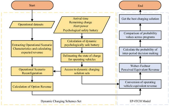
Figure 1.
EP-ITCH charging model based on WFL.
(1) Construction of Dynamic Solution Sets and Calculation of EOVs Revenue
Combining the processing and analysis of the typical daily operating EOV owner income data set, we model the operating process of EOVs, extract and quantify the operating characteristics of EOVs, and construct a revenue framework for the operating scenarios of EOVs.
Considering the factors such as arrival time, remaining power, and alert power threshold, the dynamic psychological safety power is calculated to divide the charging demand of operational vehicles under different peak and off-peak electricity pricing; then, we can calculate the revenue of different scenarios under the revenue framework of operation scenarios, and the dynamic charging scheme set is constructed.
(2) An EP-ITCH Charging Model for EOVs
To comprehensively measure the relationship between the dynamic charging scheme revenue and charging time, we consider the phenomenon that EOV owners have a perceptual attenuation of the operational revenue in their daily operation. We construct a psychological scale based on the WFL and establish an EP-ITCH charging model.
3. Construction of Dynamic Charging Scheme Set for EOVs
3.1. Preprocessing the Historical Data
To extract the operational features of the historical data, the whole day is segmented into time slices with intervals of ε duration (in particular, ε = 10 min in this study), and the frequencies of all the operational events occurring in the corresponding time period for each slice in the historical data are counted. Thus, a typical-day historical passenger order frequency table can be constructed. Then, we can reformulate the operational process using the frequency table and the operational events. The frequency and corresponding features are defined below.
We define the frequency of the operational event mw,h,i as fw,h,i, where fw,h,i is derived from the typical daily operational events table Fw×h×i extracted from historical data. w (w∈{ 1, …, ζ}) is the index of current slicing interval; h is the event type, which, in this study, was defined as the duration of the event; here, set H = {1, 2, …, k} (the duration each element in the set H can be calculated as k × 10 min, and particularly for the simplicity of the problem, = 6 in this study), h ∈ H; i ∈ {0,1}, in which 0 and 1 denote without/with a passenger, respectively, e.g., f2,3,1 represents the frequency of a passenger-carrying event lasting 30 min that occurred during the second time slice.
3.2. Reconstruct the Operational Scenarios Revenue Framework
In charging decision making, the EOV owner faces a dilemma between two symmetrical schemes: (1) charging immediately at time t1 to obtain the revenue of an equivalent charging duration Tc at a future time t2; or (2) charging at a future time t2 to obtain the revenue of an equivalent charging duration Tc immediately at time t1.
The first scheme reduces concerns regarding battery depletion by promptly initiating the charging process. However, it does carry the potential risk of revenue loss due to the uncertainty surrounding future revenue. On the other hand, the alternative scheme poses the risk of future battery depletion in exchange for immediate revenue retrieval. To make informed decisions, decision-makers (DMs) must first reconstruct the operational scenarios. This involves evaluating the equivalent operational revenue associated with two charging moments, t1 and t2, as well as the charging time Tc.
The operational time Tc can be segmented into several scenarios, each consisting of a unique combination of operational events mw,h,i. To reconstruct the operational scenarios and calculate the expected revenue J within the operational duration, three features are required: (1) the frequency of events occurring in each scenario; (2) the probability of each operational scenario; and (3) the average revenue of each operational event. The following provides detailed steps as shown in Figure 2.
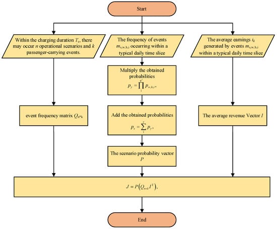
Figure 2.
Scenarios revenue framework.
Step 1. The event frequency matrix Qn×k within the operational duration
The operational scenarios s (where s ∈ S, S = {1, …, n}) can be decoupled into several repeatable permutations of independent events ms,w,h,i. The sum Σh of the durations h of all independent events in s scenarios equals the operational scenario duration. Therefore, the event frequency matrix Qn×k is arrived at, consisting of k passenger-carrying events for each one in n scenarios. Qn×k can be expressed as follows:
where qn,k denotes the frequency of the kth passenger-carrying event in the sth scenario.
Step 2. The scenario probability vector P
To calculate the possibilities of each event ms,w,h,i in operational scenario s, the frequency fw,h,i of the historical event is concerned.
Given the charging arrival time Ta and charging duration Tc, the time slices when charging starts and ends can be obtained from the table Fw×h×i, which contains ζ slices.
where pw,h,i is the possibility of mw,h,i and fw is the total occurrences of all events that may possibly occur within the remaining operational time.
Knowing the types and the occurrences q′ (total occurrences of all the events in current scenario) of events ms,w,h,i under corresponding scenarios of the charging time Tc, these independent operational events can be modeled as the irretrievable “fetching-ball experiment” procedure. For each experiment, the balls are taken out one by one (an operational event happens), and the sequence of the balls is recorded (the sequence of operational events is recorded). When all of the balls (events) are taken out (all events happen), the experiment completes (a possible combination of the events under one scenario). The “fetching-ball experiment” is repeated until no new sequences () are generated. Thus, the probabilities of each operational scenario under all possible combinations (Ps) are recorded and calculated.
Then, the scenario probability vector P is shown below:
Step 3. The average revenue vector I is shown below:
where ik is the average revenue generated by the kth passenger-carrying event during the Tc time period, as obtained from historical data.
Step 4. The expected return J is shown below:
The expected revenue J is reconstructed by combining the three features extracted from the historical operational data, which represent the operational behavior for time duration Tc.
3.3. Charging State Analysis of EOVs
Since EOVs are usually operated by both day-shift drivers and night-shift drivers, and the capacity of the vehicle batteries is limited, charging usually occurs several times in a day. Given that night-shift drivers typically charge their vehicles after their shifts end in the early morning, this study focuses on the EV charging during daytime hours.
The EV charging hours Tc are usually defined as follows:
where W is the rated capacity of the vehicle battery; BN is the initial battery state of charge (i.e., remaining charge) when arriving at the station; Blea is the battery state of charge upon completion of charging; PEV is the EV charging power; and θc is the EV charging efficiency [26].
Assuming that Bsaf is the dynamic psychological safety battery of each EOV owner for its remaining charge, and Bmin is the alert power threshold at which the vehicle battery must be charged immediately, when the remaining charge BN upon arrival is larger than Bsaf, the owner chooses not to charge. When it is lower than Bsaf, the owner chooses to charge to a value state that ensures the charge at turnaround time is greater than Bmin. Bsaf varies with the time period during the owner’s daily operation. The computation of Bsaf is established as follows.
where Vc is the average charging speed.
For charging demand, the charging time can be expressed as follows:
where Td is the number of minutes from the start of operation to the end of the shift on the current day; Ta is the time of the owner’s arrival at the charging station; Vr is the average discharge rate; and W is the capacity of the vehicle battery. It is necessary to ensure that the remaining charge at the end of charging is not less than Bsaf.
The charging duration is related to the charging start moment, the remaining charge, and Bsaf. While different DMs prefer different values of Bsaf, different charging durations are derived from Equation (9). Additionally, the peak and off-peak pricing electricity prices are also important influencing factors. The whole day is divided into multiple charging decision intervals based on the peak and off-peak pricing periods (in the following text, the peak electricity price periods will be referred to as peak periods, and the flat electricity price periods will be referred to as flat periods). When BN < Bsaf, the EOV owners contemplate charging. At this point, the charging schemes that EOV owners can choose form a dynamic set, as the number of schemes in the set varies due to the different time points at which each owner generates charging ideas; In addition, the charging scheme is influenced by various factors, including {Bsaf, Ta, BN, Tc, J, D}, where J represents the expected benefit calculated based on Tc and D represents the charging cost calculated based on Tc. These schemes, influenced by changes in Bsaf, constitute the set of dynamic charging schemes for EOVs. The dynamic charging scheme set is established as follows.
Scheme 1 is defined as charging immediately upon contemplating the need to charge. Some EOV owners may prefer to first accrue operational revenue before considering charging; thus, Scheme 2 involves waiting until the next charging decision interval to initiate charging. Instances where charging is postponed based on the owner’s preferences constitute the scenario of first obtaining operational revenue before charging. Scheme 3 involves waiting until the subsequent charging decision interval, and this pattern continues to generate multiple alternative schemes. When the shift time falls within a specific charging decision interval, where BN approaches Bmin, the EOV owners must execute a charging operation. Therefore, the scheme corresponding to this decision interval becomes the final scheme.
4. EP-ITCH Model
4.1. ITCH Model for Charging EOVs
The ITCH model refers to the process of weighing the costs and revenue of values at different moments, and then making a choice. For EOV owners, immediate charging reduces range anxiety but risks losing current revenue, while symmetrically delayed charging risks running out of battery power to gain potentially greater revenue. Therefore, this is a typical ITCH problem.
As shown in Figure 3, we defined two alternative charging intervals, u and v, in which tv > tu and xv > xu. If while charging at the time of tu, a gain of xu is obtained, then charging at the time of tv helps us earn xv. The different choices fall into symmetrical operational behaviors. Therefore, DM faces the dilemma problem of choosing to charge now and obtain revenue later, or to obtain revenue now but charge later.
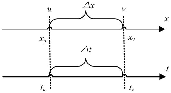
Figure 3.
ITCH charging dilemma problem for EOV owners.
From the perspective of the two symmetry schemes for the DM, revenue xu is expressed as the sum of the order revenue Jv obtained in interval v and the avoidable charging cost Dv in interval v. Then, the revenue xu and xv are given by the following:
where Ju and Jv denote the expectancy order revenues in interval u and interval v, respectively; Du and Dv denote the charging costs in interval u and interval v, respectively; and Ec represents the electricity price for the corresponding time period.
Let us define the inter-period probability P(LL) of the owner’s charging choice as follows:
where x* = (xu + xv)/2, t* = (tu + tv)/2, and L (•) = 1/(1 + e−•) is the cumulative distribution function of the logistic distribution with mean 0 and variance 1, and β1, βxA, βxB, βtA, and βtR are the weights. When the value of P(LL) is greater than σ, the option with a larger revenue at a later moment is selected. Otherwise, the option with lower revenue at an earlier moment is selected.
4.2. WFL of Perception
The WFL is a law that indicates the relationship between psychological and physical quantities and can characterize the nonlinear perceptions of DMs. For moderate stimuli, the response level η of the human body is proportional to the logarithm of the objective stimuli φ and is expressed as follows:
where η denotes a natural number such that η = 0, …, α, with α representing the maximum response level on the psychological scale. The term φη is defined as the psychological scale threshold corresponding to the physical intensity threshold that is perceived at a response level of η, where c is the constant of proportionality, and φ0 is the smallest physical intensity that can be felt.
Given a response level of η, it follows from the above equation that φη is given by the following:
By substituting all values of η, one can obtain the psychological scale that manifests the intensity of an individual’s psychological response.
In this study, the passenger-carrying events with the lowest and the highest revenue per passenger are defined as imin and imax, respectively, corresponding to the minimum physical intensity φ0 and the psychological scale threshold φa in Equation (15), respectively. From this, the psychological scale of the EOV owner’s perception of revenue can be established.
Furthermore, to account for the variability in DMs’ sensitivity to revenue, psychological scales reflective of their heterogeneous sensitivity can be constructed by choosing different response levels η.
4.3. EP-ITCH Charging Model
Due to an owner’s perceptual attenuation of operational revenue, the owner’s revenue x for their charging decision can be processed using the psychological scale thresholds as boundaries for segmented perception. The flowchart of the EP-ITCH charging model is shown in Figure 4. The two charging schemes involved in each decision include two elements, which are time and revenues.
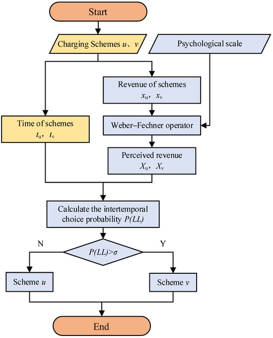
Figure 4.
Flowchart of the Weber–Fechner-based EP-ITCH charging model.
We define the Weber–Fechner operator for computing the perceived revenue X as follows:
where x represents the revenue within the charging duration Tc.
By substituting the results of the operator calculations into Equation (12), it yields the following:
with
where P(LL) represents the probability of opting for “the smaller, closer option”. By default, when the value of P(LL) exceeds σ, the choice of the DM falls on charging in interval u; conversely, when the value of P(LL) is less than σ, charging in interval v is selected.
5. Case Study
5.1. Data Preparation
The time periods in this case were divided with reference to the peak and off-peak electricity pricing in a certain city in southern China. We set the study time as 9:00–16:00. The time segments were defined as follows: 9:00–10:00 as the flat period T1, 10:00–12:00 as the peak period T2, 12:00–14:00 as the flat period T3, and 14:00–16:00 as the peak period T4. The charging schemes available to the owners were divided as shown in Table 2. In addition, the parameter settings for the different time periods in this study are shown in Table 3.
Table 2.
Charging schemes table.
Table 3.
Parameterization.
According to the research, the BYD E6 EV is a widely used EOV in the city, with a battery capacity of 45 kWh [27]; the charging stations in the city have a charging power of 35 kW [28], with a charging efficiency of θc of 0.95 [29].
For the starting time of charging Ta, we fit a distribution based on the vehicle quantity curve in the commercial scenario described in reference [30]. We obtained an extension of the normal distribution known as the epsilon-skew normal distribution, which includes an additional parameter to control its skewness. The epsilon-skew normal distribution function is used as the probability density function for the starting time of charging for EOVs.
where φt and Φt are the probability density function and cumulative distribution function of the standard normal distribution, respectively.
For the power data, to ensure that the situation in the scheme exists, there are upper and lower limits on the residual power BN, which are taken uniformly within the power limit and are recorded in fractional form. That is, 0.5 represents 50 percent of the charge.
When using psychological scales, we defaulted to a psychological scale with α = 7 (Figure 4), with a maximum guest revenue of 134.7 and a minimum guest revenue of 10.
According to [18], in the ITCH model, the default parameters are set to β1 = 0, βxA = 0.1, βxB = 0.1, βtA = −0.1, βtR = −0.1, and σ = 0.5.
For calculating the passenger revenue of EOVs according to the EOVs charge standard of a city in the south, the billing formula can be obtained as follows:
where Rprice is the cost of the passenger order, G is the actual mileage driven by the passenger order, the unit of revenue of the passenger order is CNY, and the unit of operating mileage is meters.
5.2. Case Design
The dataset used in this study consists of over 40,000,000 rows of historical operational data of over 1800 EOVs in a southern city in China, including car ID, time, latitudinal and longitudinal coordinates, and with/without passenger status. The coordinates were recorded using the WGS84 coordinate system.
The effectiveness of the proposed model in solving the multi-time-span decision-making problem was verified by horizontally comparing the charging decision-making results of the expected utility theory (EUT), the ITCH model, and the EP-ITCH model. The effectiveness of the proposed model in quantifying the influence of irrational and objective factors was verified by vertically comparing the charging decision results of different psychological scales in the EP-ITCH model and under different electricity prices.
We completed the feature extraction of the frequency operational events, the probability of each operational scenario, and the average revenue of each operational event mentioned in Section 3. This was achieved by writing SQL programs in ClickHouse. In Section 4, we established the EP-ITCH model by writing macro programs in Excel, along with conducting the necessary calculations and analysis. Finally, all of the plotting was completed using Origin.
The structure of the case design is shown in Table 4.
Table 4.
Case structure.
Case I: Charging decision analysis under three different models.
Besides the conventional EUT model [11], the ITCH [19] and EP-ITCH models were employed to model and analyze the charging problem of EOVs. A comparative analysis was conducted on the final charging schemes chosen by EVO owners under the three models, as illustrated in Figure 5.
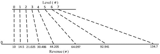
Figure 5.
Psychological scale with α = 7.
In Situation 1 (Figure 6), the fully rational owner under the EUT model will choose the scheme with the largest revenue, prioritizing Scheme 3 > Scheme 2 > Scheme 1. The growth of the remaining power BN has a limited impact on this choice.
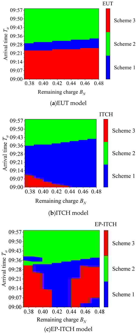
Figure 6.
Schematic comparison of charging decision results under the three models for Situation 1.
On the other hand, the ITCH model introduces weight parameters to model the value of the impact of revenue and time, which provides a tool for modeling irrational decision-making behavior [19]. By default, the ITCH model shows that a DM will be more inclined to choose the charging scheme with larger revenues and lower time costs. Since Scheme 1 has the lowest time cost, it becomes increasingly likely to be chosen. This effect becomes even more pronounced as the remaining power BN increases.
The Weber–Fechner operator in the EP-ITCH model grades the difference between expected returns, leading to two phenomena:
1. When the perceived expected benefits exceed the perceived threshold, the disparity in benefits increases, which raises the probability of choosing the first charging option.
2. When the perceived expected returns are similar, differences in the expected returns are smoothed out, highlighting the impact of electricity costs on decision making.
Compared to the ITCH model without considering perceptual attenuation, a DM under the EP-ITCH model tends to choose charging schemes with lower average electricity prices and larger equivalent perceived revenues. The differences in the choices of the EP-ITCH model are because EP-ITCH introduces the Weber–Fechner operator to describe the perceptual attenuation in decision making, which leads to irrational factors in decision making. Therefore, it can capture irrational behaviors in decision making more accurately.
In Situation 2 and Situation 3, since the revenue decreases significantly with increased time, a DM will undoubtedly choose to charge immediately with Scheme 1, which comes with larger revenues and earlier times, and there is no difference in the owner’s decision under the three models.
To sum up, the fully rational owner under the EUT will directly choose the charging scheme with larger revenues, and the growth of the remaining power BN has little effect on the choice. Partially rational owners under the ITCH model will hesitate under the two options of “smaller revenue and earlier time” and “larger revenue and later time”, because of immediate gratification. Compared with the EUT, the ITCH model takes into account the problem of time cost between the time spans of the different schemes, so that EOV owners are more inclined to choose the charging scheme with higher gains and smaller time costs, and the weakening effect of the instantaneous effect will gradually become obvious with the growth of the BN. The EP-ITCH model describes the phenomenon that the owner has an attenuated grading of the subjective perception of revenue, and EOV owners will be more inclined to choose the charging scheme with a lower average electricity price and higher equivalent perceptual revenue.
Case II: Analysis of different psychological scales on EOV owners’ charging decisions
To compare the differences in charging decisions of owners with varying perceptual acuity, the psychological scales of low acuity (α = 6) and high acuity (α = 9) were incorporated herein. The operational time remained 9:00–16:00 h to obtain the charging decisions of owners with three different psychological scales. Since it is known in Case I that in Situation 2 and Situation 3, all of them will choose Scheme 1, which has larger revenue at an earlier time; only the change in the psychological scales under Situation 1 was discussed in Case II.
In the EP-ITCH model, the decision is determined by time and revenue, and the revenue consists of expected returns and average electricity costs. Since the psychological scale grades the expected return, changes in the expected return under Situation 1 are analyzed first. According to the typical data analysis, the expected return is in the range of CNY 30–50 and decreases gradually with the growth of Ta and BN.
The expected returns with the same threshold in psychological scale were transformed into perceived expected return through the Weber–Fechner operator, which are perceived as the same perceived expected return. When we focus on the change in average electricity cost in Situation 1, several conclusions can be drawn.
When we focus on the arrival time Ta, the trend in electricity fee variation is illustrated in Figure 7.
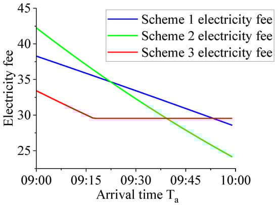
Figure 7.
BN = 0.37227, the trend in electricity fee varies with Ta.
When Ta is small, Scheme 2 will charge during peak hours or start from peak hours and end in flat hours. Thus, Scheme 3 is chosen, because its average electricity cost is initially lower than that of Schemes 1 and 2.
When the charging decision time Ta is postponed, the peak-to-flat ratio of the average electricity cost calculation changes, resulting in an increase in the peak period ratio of Scheme 1, and the electricity cost gradually exceeds that of Scheme 2. The relationship between the average electricity costs of the schemes becomes Scheme 1 > Scheme 2 > Scheme 3.
When Ta increases to a certain value, one needs to charge for extra time to reach the dynamic psychological safety battery Bsaf, which supports the operation of the vehicle until handover time. Therefore, Scheme 3 will experience extended charging time, and its charging time Tc will increase, as well as the electricity cost, when the electricity cost of Scheme 3 exceeds that of Scheme 2 and Scheme 1. The final relationship between the average electricity costs of the schemes becomes Scheme 1 > Scheme 3 > Scheme 2.
When we focus on the remaining battery power BN, the trend in electricity fee variation is illustrated in Figure 8.
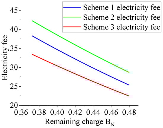
Figure 8.
Ta = 9:00, the trend in electricity fee varies with BN.
When BN increases, Tc becomes shorter, and the difference in the average cost of electricity between the schemes decreases.
When α = 6 (Figure 9a), the EOV owner’s sensitivity to the expected return is lowest compared with the case where α is greater than 6.
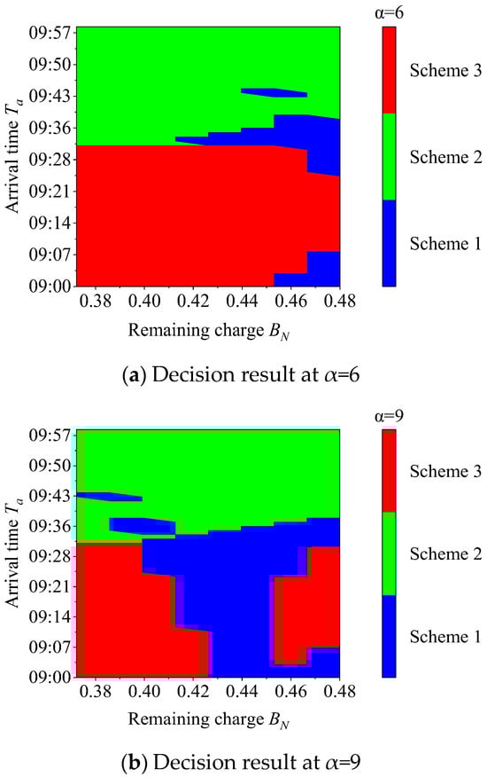
Figure 9.
EP-ITCH results under different psychological scales for Situation 1.
In this case, the weight of the electricity cost is much greater than that of the revenue. When Ta and BN are smaller, Tc is longer because of a smaller BN, resulting in a large gap between the revenue of each scheme. Compared to the revenue, the influence of the time cost can be ignored; Scheme 3, which has low electricity costs and large revenues is the best option.
When BN is fixed and Ta increases, decision making will prioritize Scheme 2 due to its lower electricity costs.
When Ta is fixed and BN increases, the probability of choosing Scheme 1 increases due to the reduced difference in electricity costs and the impact of time costs.
When α = 7 (Figure 6), the owner’s sensitivity to revenue increases, and the effect of the psychological scale thresholds on the expected return gradually emerges. When Ta is in the 9:00–9:30 time period and BN is in the 0.38–0.46 battery power interval, the expected return of different schemes will locate between two different levels of 3 (30.486–44.205) and 4 (44.205–64.097) in the α = 7 psychological scale, which widens the gap of the revenue between the schemes, at which point the time cost effect is insufficient to compensate for the gap between the revenues, and the probability of choosing Scheme 1 with the largest perceived revenues increases.
When α = 9 (Figure 9b), the larger revenue difference between the schemes makes the time cost impact insufficient to compensate for it. Thus, the decision tends to favor the scheme with the highest perceived revenue. For example, when Ta is in the 9:00–9:30 time period and BN is in the 0.39–0.48 range, the expected return of the different schemes will be in the α = 9 psychological scale between the two different levels of 4 (32.24–43.2) and 5 (43.2–57.89). In this case, Scheme 1 comes with the greatest revenue; therefore, Scheme 1 is chosen over the other two options.
The results show that in Situation 1, as the level of the psychological scale increments, the more the expected return is graded by the psychological scale, the higher the probability that the scheme of charging first and obtaining later is selected. The results show that decision making is influenced by the thresholds of perception, which exhibit significant irrational characteristics. Different psychological scales that represent different sensibilities result in different irrational decision-making options.
Case III: Charging decision analysis and power shift of EOV owners subject to different electricity prices
As it is known from previous cases that the price of electricity influences decision making, it is valuable to discuss the differences in charging decisions under different electricity prices. The operational time was kept at 9:00–16:00, in order to obtain the charging decisions of owners under different electricity prices, and the change in average electricity cost in Situation 1 was analyzed, as shown in Case II.
In Figure 10, we can see that the probability of choosing Scheme 2 under electricity at twice the price increases when Ta is in the 9:30–9:59 time period compared to the original price, which is consistent with the trend that the prices of Scheme 2 are eventually become lower than the other schemes when Ta is delayed; the probability of choosing Scheme 3 under electricity at twice the price increases when Ta is in the 9:00–9:40 time period, and BN is in the ranges of 0.38–0.43 and 0.44–0.48 compared to the original price. The probability of Scheme 3 increases, which is consistent with the pattern that was discussed in Case II.
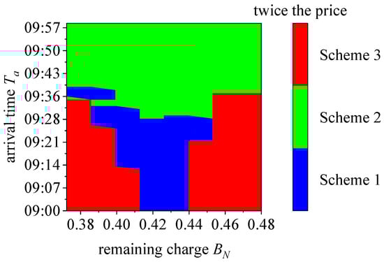
Figure 10.
EP-ITCH results under different electricity prices for Situation 1.
In Situation 1, with the increase in electricity prices, the difference in revenue becomes larger. However, compared with the significant changes in electricity costs, the time cost change remains constant, and its impact on decision making is greatly reduced. Therefore, the probability of choosing the scheme with the lowest average electricity cost increases.
To better observe the impact of differentiated electricity price settings on the charging behavior of EOV owners and the impact of the settings on the power grid, we plotted the cumulative charging load curves (Figure 11) of EOV clusters under different electricity price settings.
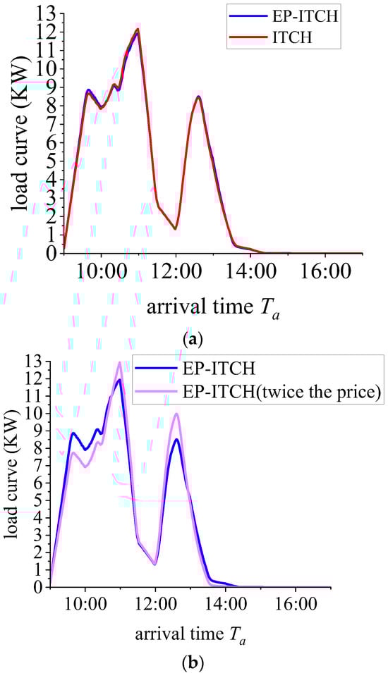
Figure 11.
Load profiles under different tariffs in the ITCH model and the EP-ITCH model. (a) The comparison of load curves between EP-ITCH model and ITCH model under default the prices. (b) The comparison of the load curves of the EP-ITCH model under default the prices and double the prices.
Under the EP-ITCH model, compared with the original electricity price, the load transfer at double the electricity price is shown in Table 5. The load demands in the two time periods of 9:00–10:47 and 12:57–17:00 are transferred to 10:48–12:56. Under the ITCH model, compared with the original electricity price, the load transfer at double the electricity price is shown in Table 6. The load demands in the two time periods of 9:00–10:47 and 12:58–17:00 are transferred to 10:48–12:57.
Table 5.
EP-ITCH modeling load shifting volume.
Table 6.
ITCH modeling load shifting volume.
From the load curve, compared to the ITCH model, the load under the EP-ITCH model is shifted from the peak hours to the flat hours. It can be seen from the amount of load transfer that, due to the increase in the gap between the revenues of higher electricity prices, the objective factor of time cost reduces the charging cost impact on the owner, and the owner is more inclined to obtain revenues first and then charge, so the load demand is shifted backward. The load reaches a peak at 11:00, which is in line with the law of electricity consumption during peak hours, but due to the impact of peak hours electricity prices, the load demand growth is not large; due to the price of electricity entering into the usual section at 12:00, and considering the increased possibility of EOV owners obtaining revenue first and charging later, compared with the original price, the load demand of the 2-fold price rises sharply around 12:40.
From Table 7 and Table 8, it is evident that with the same model, an increase in electricity price exacerbates grid fluctuations. When electricity prices are the same, compared to the ITCH model, the EP-ITCH model exhibits smaller peak–valley differences and grid fluctuation variances. Therefore, the charging decision model proposed in this study results in smaller fluctuations for the grid and has less of an impact on grid stability.
Table 7.
The load peak–valley difference under different electricity prices for the ITCH and EP-ITCH models.
Table 8.
The load fluctuation variance under different electricity prices for the ITCH and EP-ITCH models.
The results show that compared with the use of the ITCH model, the EP-ITCH model can, to a certain extent, help EOV owners avoid peak electricity consumption, improve their economic revenue, promote the rational utilization of charging equipment and electric power resources, and attenuate the impacts of large-scale EOV grid connections on the network. At the same time, in the EP-ITCH model, through the reasonable regulation of price changes, the load side of the regulation and scheduling can be realized.
6. Conclusions
By combining objective constraints on charging behavior decisions across multiple time spans with the subjective perception of vehicle owners, this study comprehensively assessed the relationship between revenues and time costs. It established an EOV equivalent perception intertemporal decision-making charging model based on WFL. Validation through simulations was conducted using transportation data from a southern city in China, leading to the following conclusions:
(1) Charging Scheme Selection Analysis:
Unlike the EUT model, which only considers revenues, the ITCH model incorporates both revenues and time costs. Within this framework, decision-makers are more inclined to choose charging schemes that offer higher revenues and lower time costs. Thus, EOV owners are more likely to select Scheme 1, which has the lowest time costs, especially when the remaining battery level (BN) increases.
The EP-ITCH model integrates the WFL method to account for irrational factors in decision making, explaining the DMs’ perception attenuation of revenue. This model makes DMs more likely to choose schemes with lower average electricity prices and higher perceived revenues.
(2) Decision-Influencing Factor Analysis:
In the EP-ITCH model, the influence proportions of expected revenue and average electricity price exhibit irrational characteristics with changes in the psychological scale level. Different psychological scales represent EOV owner groups with different sensitivities to income changes.
When the income is the same, EOV owners who are more sensitive to income changes are more influenced by the expected revenue in their decision making, and they tend to choose to charge first, then obtain revenue.
If EOV owners are not sensitive to income changes, the average electricity price and time significantly affect their decision making, and they prefer to charge during periods with lower electricity prices and the lowest time cost.
(3) Impact Analysis of different Electricity Prices:
After a price increase, the influence of revenue on decision making increases, and DMs are more inclined to obtain revenue first, then charge.
It can be seen from the analysis of load demand under different models and different electricity prices that the EP-ITCH model has smaller load peak–valley differences and load fluctuation variances, indicating that the charging decisions made by the model are more conducive to stable operation of the power grid, which demonstrates the superiority of the model.
Author Contributions
In the writing of this article, Y.H.,Y.Q. and P.L. contributed the most, followed by B.F. and M.X.; conceptualization, Y.Q. and B.F.; methodology, Y.H.; software, Y.Q.; validation, Y.H.,Y.Q., P.L. and B.F.; formal analysis, Y.Q.; investigation, M.X.; resources, Y.Q. and B.F.; data curation, Y.Q.; writing—original draft preparation, Y.H. and P.L.; writing—review and editing, Y.Q., H.Z. and B.F.; visualization, Y.H. and P.L.; supervision, B.F. and M.X.; project administration, B.F. and Y.H.; funding acquisition, B.F. All authors have read and agreed to the published version of the manuscript.
Funding
This work was supported by the Key Research and Development Program of the Hubei Province of China (Grant No. 2021BAA193). The grant is gratefully acknowledged.
Data Availability Statement
The data presented in this study are available on request from the corresponding author. The data are not publicly available due to multiple authors and the confidentiality requirements of the authors’ organizations.
Conflicts of Interest
The authors declare no conflicts of interest.
Appendix A
Table A1.
The related definition of symbols.
Table A1.
The related definition of symbols.
| Notation | Parameters | Unit |
|---|---|---|
| Index of current slicing interval | w | minute |
| The duration of the operational event | h | minute |
| Without/with passenger | i | |
| Operational scenarios | s | |
| Number of scenarios | n | |
| passenger-carrying events | k | |
| Events sequences | γ | |
| Time slices | ε | minute |
| Operational event | m | |
| Frequency of operational events | f | |
| Charging time | Tc | minute |
| Expected revenue | J | yuan |
| Event frequency matrix | Qn×k | |
| The scenario probability vector | P | |
| Probability of operational scenarios | Ps | |
| Average revenue Vector | I | yuan |
| Rated capacity of vehicle battery | W | kW·h |
| Remaining charge | BN | kW·h |
| Charge completed battery level | Blea | kW·h |
| Charging power of EVs | PEV | kW |
| Charging efficiency of EVs | θc | |
| Dynamic psychological safety battery | Bsaf | kW·h |
| Alert power threshold | Bmin | kW·h |
| average charging speed | Vc | kW·h/min |
| Full day operation time | Td | minute |
| Arrival time at charging station | Ta | minute |
| average discharge rate | Vr | kW·h/min |
| Charging cost | D | yuan |
| Charging period v | tv | minute |
| Charging period u | tu | minute |
| Expected revenue v | xv | yuan |
| Expected revenue u | xu | yuan |
| Order revenue v | Jv | yuan |
| Order revenue u | Ju | yuan |
| Charging costs in period v | Dv | yuan |
| Charging costs in period u | Du | yuan |
| Inter-period probability | P(LL) | |
| Average revenue | x* | yuan |
| Average time | t* | minute |
| Intercept | β1 | |
| The weight of absolute returns | βxA | |
| Weight on relative returns | βxB | |
| The weight of absolute time | βtA | |
| Weight on relative time | βtR | |
| Logical distribution function | L | |
| Discriminant threshold | σ | |
| Response level | η | |
| The psychological scale threshold Corresponding to level η | φη | |
| Smallest physical intensity | φ0 | |
| Constant of proportionality | c | |
| WFL operator | X | |
| Average equivalent perceived revenue | A* | yuan |
References
- Liu, H.; Li, Y.; Zhang, C.; Li, J.; Li, X.; Zhao, Y. Electric Vehicle Charging Station Location Model considering Charging Choice Behavior and Range Anxiety. Sustainability 2022, 14, 4213. [Google Scholar] [CrossRef]
- Zagrajek, K.; Kłos, M.; Rasolomampionona, D.D.; Lewandowski, M.; Pawlak, K. The Novel Approach of Using Electric Vehicles as a Resource to Mitigate the Negative Effects of Power Rationing on Non-Residential Buildings. Energies 2023, 17, 18. [Google Scholar] [CrossRef]
- Cui, Y.; Hu, Z.; Duan, X. Review on the Electric Vehicles Operation Optimization Considering the Spatial Flexibility of Electric Vehicles Charging Demands. Power Syst. Technol. 2022, 46, 981–994. [Google Scholar]
- Rivas, A.E.L.; Abrao, T. Faults in smart grid systems: Monitoring, detection and classification. Electr. Power Syst. Res. 2020, 189, 106602. [Google Scholar] [CrossRef]
- Meiers, J.; Frey, G. A Case Study of the Use of Smart EV Charging for Peak Shaving in Local Area Grids. Energies 2023, 17, 47. [Google Scholar] [CrossRef]
- Debnath, B.; Biswas, S.; Uddin, M.F. Optimization of electric vehicle charging to shave peak load for integration in smart grid. In Proceedings of the 2020 IEEE Region 10 Symposium (TENSYMP), Dhaka, Bangladesh, 5–7 June 2020; IEEE: Piscataway, NJ, USA, 2020; pp. 483–488. [Google Scholar]
- Valogianni, K.; Ketter, W.; Collins, J.; Zhdanov, D. Sustainable electric vehicle charging using adaptive pricing. Prod. Oper. Manag. 2020, 29, 1550–1572. [Google Scholar] [CrossRef]
- Chen, H.; Zhao, X. Research on Electric Vehicle Charging Optimization Considering Distributed Photovoltaic Power Generation. Chin. J. Manag. Sci. 2023, 31, 161–170. [Google Scholar] [CrossRef]
- Wang, H.; Zhang, M.; Yang, X. Electric vehicle charging demand forecasting based on influence of weather and temperature. Electr. Meas. Instrum. 2017, 54, 123–128. [Google Scholar]
- Al-Alwash, H.; Borcoci, E. Optimal Charging Scheme for Electric Vehicles (EVs) in SDN-based Vehicular Network, Scheduling, and Routing. In Proceedings of the 2022 14th International Conference on Communications (COMM), Bucharest, Romania, 16–18 June 2022; pp. 1–8. [Google Scholar]
- Feng, W.; Quan, Y.; Fu, B.; Zhao, N.; Li, C.; Lu, J. Decision-making model for charging of operational Evs based on adapted cumulated prospect theory. Electr. Power Eng. Technol. 2023, 42, 170–179. [Google Scholar]
- Chakraborty, A. Present bias. Econometrica 2021, 89, 1921–1961. [Google Scholar] [CrossRef]
- Clairand, J.-M.; Rodriguez-Garcia, J.; Alvarez-Bel, C. Smart charging for electric vehicle aggregators considering users’ preferences. IEEE Access 2018, 6, 54624–54635. [Google Scholar] [CrossRef]
- Ensslen, A.; Ringler, P.; Dörr, L.; Jochem, P.; Zimmermann, F.; Fichtner, W. Incentivizing smart charging: Modeling charging tariffs for electric vehicles in German and French electricity markets. Energy Res. Soc. Sci. 2018, 42, 112–126. [Google Scholar] [CrossRef]
- Wang, S.; Bi, S.; Zhang, Y.-J.A.; Huang, J. Electrical vehicle charging station profit maximization: Admission, pricing, and online scheduling. IEEE Trans. Sustain. Energy 2018, 9, 1722–1731. [Google Scholar] [CrossRef]
- Chung, H.M.; Li, W.T.; Yuen, C.; Wen, C.-K.; Crespi, N. Electric vehicle charge scheduling mechanism to maximize cost efficiency and user convenience. IEEE Trans. Smart Grid 2018, 10, 3020–3030. [Google Scholar] [CrossRef]
- Leng, J.-Q.; Zhai, J.; Li, Q.-W.; Zhao, L. Construction of road network vulnerability evaluation index based on general travel cost. Phys. A Stat. Mech. Its Appl. 2018, 493, 421–429. [Google Scholar] [CrossRef]
- Engelson, L.; Fosgerau, M. The cost of travel time variability: Three measures with properties. Transp. Res. Part B Methodol. 2016, 91, 555–564. [Google Scholar] [CrossRef]
- Marzilli Ericson, K.M.; White, J.M.; Laibson, D.; Cohen, J.D. Money earlier or later? Simple heuristics explain intertemporal choices better than delay discounting does. Psychol. Sci. 2015, 26, 826–833. [Google Scholar] [CrossRef]
- Yang, L.; Sheng, L.; Yuqiang, L.; Junwei, L.; Yuheng, C. Technology Research on Panoramic Situation Awareness of Operation State of Smart Distribution Network. IOP Conf. Ser. Earth Environ. Sci. 2021, 645, 012007. [Google Scholar] [CrossRef]
- Arslan, T. A Psychometric Approach to the VIKOR Method for Eliciting Subjective Public Assessments. IEEE Access 2020, 8, 54100–54109. [Google Scholar] [CrossRef]
- Hou, H.; Wang, Y.; Wu, X.; Chen, Y.; Huang, L.; Zhang, R. MCharging and discharging scheduling strategy for electric vehicles taking into account the psychological effect of range anxiety on a long-term scale. High Volt. Technol. 2023, 49, 85–93. [Google Scholar]
- Long, X.; Yang, J.; Wu, F.; Zhan, X.P.; Lin, Y.J.; Xu, J. Electric Vehicle Charging Load Prediction Considering Road Network-Electric Network Interaction and User Psychology. Autom. Electr. Power Syst. 2020, 44, 86–93. [Google Scholar]
- Zhang, Y.; Hou, H.; Huang, J.; Zhang, Q.; Tang, A.; Zhu, S. An optimal subsidy scheduling strategy for electric vehicles in multi-energy systems. Energy Rep. 2021, 7, 44–49. [Google Scholar] [CrossRef]
- Li, J.; Liang, C.; Liu, K.; Han, W.; Liang, X.; Li, X. Optimal Scheduling Strategy for Electric Vehicles Charging and Discharging Considering User Responsiveness. South. Power Syst. Technol. 2023, 17, 123–132. [Google Scholar]
- Li, H.; Du, Z.; Chen, L.; Guan, L.; Zhou, B. Electric Vehicle Charging Load Prediction Model and V2G Assessment Based on Travel Simulation. Autom. Electr. Power Syst. 2019, 43, 88–96. [Google Scholar]
- Ma, Y.; Ma, Z. Ordered Charging Optimization and Revenue Analysis of Electric Vehicles Based on Game Algorith. Electr. Power Eng. Technol. 2021, 40, 10–16. [Google Scholar]
- Yao, Y.; Zhao, R.; Li, C.; Yan, Z.; Xie, K. Electric Vehicle Control Strategy for Power System Flexibility. Trans. China Electrotech. Soc. 2022, 37, 2813–2824. [Google Scholar]
- Wang, Q.; Tian, Y.; Wang, J.; Hu, F.X.; Zhou, N.C. Day-Ahead to Real-Time Coordinated Optimization Model for Distribution Network Considering Reactive Power Compensation of Charging Stations. Autom. Electr. Power Syst. 2021, 45, 27–34. [Google Scholar]
- Xue, L.; Xia, J.; Yu, R.; Ren, H.; Liu, Y.; Wei, W.; Liu, P. Analysis of the Impact of Large-Scale Promotion of New Energy Vehicles on the Power Grid: How New Energy Vehicles Can Better Integrate into the Power Grid Series One. WRI China. (2020, June 1). Available online: https://wri.org.cn/research/quantifying-grid-impacts-electric-vehicles-china (accessed on 2 March 2024).
Disclaimer/Publisher’s Note: The statements, opinions and data contained in all publications are solely those of the individual author(s) and contributor(s) and not of MDPI and/or the editor(s). MDPI and/or the editor(s) disclaim responsibility for any injury to people or property resulting from any ideas, methods, instructions or products referred to in the content. |
© 2024 by the authors. Licensee MDPI, Basel, Switzerland. This article is an open access article distributed under the terms and conditions of the Creative Commons Attribution (CC BY) license (https://creativecommons.org/licenses/by/4.0/).