Symmetric-Type Multi-Step Difference Methods for Solving Nonlinear Equations

Abstract

Symmetric-type methods (STM) without derivatives have been used extensively to solve nonlinear equations in various spaces. In particular, multi-step STMs of a higher order of convergence are very useful. By freezing the divided differences in the methods and using a weight operator a method is generated using m steps (m a natural number) of convergence order 2 m. This method avoids a large increase in the number of operator evaluations. However, there are several problems with the conditions used to show the convergence: the existence of high order derivatives is assumed, which are not in the method; there are no a priori results for the error distances or information on the uniqueness of the solutions. Therefore, the earlier studies cannot guarantee the convergence of the method to solve nondifferentiable equations. However, the method may converge to the solution. Thus, the convergence conditions can be weakened. These problems arise since the convergence order is determined using the Taylor series which requires the existence of high-order derivatives which are not present in the method, and they may not even exist. These concerns are our motivation for authoring this article. Moreover, the novelty of this article is that all the aforementioned problems are addressed positively, and by using conditions only related to the divided differences in the method. Furthermore, a more challenging and important semi-local analysis of convergence is presented utilizing majorizing sequences in combination with the concept of the generalized continuity of the divided difference involved. The convergence is also extended from the Euclidean to the Banach space. We have chosen to demonstrate our technique in the present method. But it can be used in other studies using the Taylor series to show the convergence of the method. The applicability of other single- or multi-step methods using the inverses of linear operators with or without derivatives can also be extended with the same methodology along the same lines. Several examples are provided to test the theoretical results and validate the performance of the method.

1. Introduction

Let E stand for Banach space and $D\subseteq E$ for an open set. Suppose that $P:D\to E$ is a continuous operator. A plethora of applications are thus reduced to solving the equation

$$P(x)=0.$$

(1)

A solution $x^{*}\in D$ to this equation is needed in closed form. But this is attainable only in special situations. That is why most solution approaches are iterative when a sequence is developed that is convergent to $x^{*}$ under some conditions of the operator P and the starting point $x_0\in D$.

The existence and uniqueness of the solution’s results are usually developed for an equation like (1). In this case, Equation (1) has solutions and so it is needed to present and analyze iterative methods (ITs).

No matter which IT is utilized, there are three concerns. First, the iterations must exist in the domain D. That is, if the IT requires the evaluation of an IT at all $x_k$, it must be assured that these iterates remain in the domain of the operator P. If we refer to Newton’s method, the Fréchet derivative $P^{\prime }(x_k)$ which is a linear operator as well as the inverse $P^{\prime }{(x_k)}^{-1}$ must be well defined at all $x_k$. That is why we usually provide conditions that ensure that the iterates exist provided that the IT initiates from an initial point $x_0$. Another more challenging concern is the convergence of the sequence $\{x_k\}$, and if their limits are indeed solutions to Equation (1). A plethora of such results exists [1,2]. The first one is usually called local convergence, where we start by assuming the existence of some $x^{*}\in D$, and then we provide some neighborhoods of $x^{*}$ called convergence balls such that all of the initial points are in it, and all of the iterates produced by the IT exist and converge to $x^{*}$. The second type of convergence, usually called semilocal, does not rely on the existence of the solution $x^{*}$, but it shows certain, usually difficult to verify, conditions of the operator P and the initial point $x_0$. However, under these conditions, the convergence of the sequence to $x^{*}$ is assured. In the semilocal case, we also provide computable error estimates for the distances $\parallel x_{k+1}-x_k\parallel$ or $\parallel x^{*}-x_k\parallel$, which are not given in the local convergence theorems. However, even these estimates are usually pessimistic.

A widely used single-step method is Newton’s (NA), defined as [1,3]

$$x_0\in D,x_{k+1}=x_k-P^{\prime }{(x_k)}^{-1}P(x_k).$$

The convergence order of (NA) is two [1]. But the inversion of the derivative $P^{\prime }(x_k)$ is required at each step. This inversion may not be possible or may very expensive to carry out.

The modified Newton’s method [1,2] is defined by

$$x_0\in D,x_{k+1}=x_k-P^{\prime }{(x_0)}^{-1}P(x_k).$$

This method requires only the inversion of $P^{\prime }(x_0)$. But the convergence order of it is only one.

To avoid the generally expensive computation of the Fréchet derivative $P^{\prime }(x_k)$ of the operator P and increase the convergence to be higher than one other ITs have been developed [1,3,4,5,6,7] using divided differences of order one [1,2]. The methods of chords or Regula falsi or the Secant method are some of the most used ITs for solving Equation (1). They are defined by

$$x_{-1},x_0\in D,x_{k+1}=x_k-{[x_k,x_{k-1};P]}^{-1}P(x_k),$$

where $\mathcal{L}(E,E)$ denotes the space for mappings of E into E for linear operators that are bounded, and $[·,·;P]:D\times D\to \mathcal{L}(E,E)$ is called a divided difference of order one. But the R-order of convergence is ${\displaystyle \frac{1+\sqrt{5}}{2}}$ which is larger than one but smaller than two. However, it is possible to still use divided differences and obtain a convergence order greater than ${\displaystyle \frac{1+\sqrt{5}}{2}}$.

By utilizing the symmetric difference formula

$$P^{\prime }(x)\approx [x+h,x-h;P],$$

we derive the Symmetric-Steffensen-type method (SSTM)

$$x_{k+1}=x_k-{[x_k+P(x_k),x_k-P(x_k);P]}^{-1}P(x_k),$$

which is also of convergence order two [4,5]. But the divided difference $[·,·;P]$ is used instead of the derivative $P^{\prime }$. Other Steffensen-type methods are studied in [6,7,8,9]. Generalizations of the SSTM have been suggested to increase the convergence order in combination with weight operators, and frozen derivatives.

Symmetries play a central role in the dynamics of physical systems. Quantum physics are at the core of symmetry principles. Symmetries do not only naturally appear in geometry. They appear every time that a mathematical object stays unchanged under transformations. Even and odd functions studied in calculus are examples of symmetry. Symmetric matrices or graphs are another example. Symmetries characterize the solutions of differential or integral equations. That is why it makes sense to consider iterative methods of a symmetric nature to solve such equations.

Let us revisit the family of methods defined by [5]

$$\begin{array}{ccc}\hfill u_k& =& x_k+aP(x_k),A_k=[u_k,x_k;P],\hfill \\ \hfill y_k^{(1)}& =& x_k-A_k^{-1}P(x_k),z_k=y_k^{(1)}+bP(y_k^{(1)}),\hfill \\ \hfill y_k^{(2)}& =& y_k^{(1)}-B(s_k)A_k^{-1}P(y_k^{(1)}),s_k=A_k^{-1}[y_k^{(1)},z_k;P],\hfill \\ \hfill & & \dots \hfill \\ \hfill y_k^{(m-1)}& =& y_k^{(m-2)}-B(s_k)A_k^{-1}P(y_k^{(m-2)}),\hfill \\ \hfill x_{k+1}& =& y_k^{(m)}=y_k^{(m-1)}-B(s_k)A_k^{-1}P(y_k^{(m-1)}),\hfill \end{array}$$

(2)

where $k=0,1,2,\dots$ is the number of iterations; m is the number of steps; $a,b$ are real numbers; and $B(s_k)$ is a linear weight operator [10,11]. The weight $B(s)$ is any real matrix function that satisfies $B(0)=1$, $B(1)=-1$ and $\parallel B^{″}(0)\parallel <\infty .$ The convergence order 2 m is proven in [5] using the Taylor series for $E={\mathbb{R}}^n$. A detailed favorable comparison with other competing methods using similar information has been carried out in [5,10,11]. This includes the computation of the CPU time. It is because of these advantages that we picked method (2) to demonstrate our technique. But, we noticed that there are also limitations to the approach [5,10,11].

Motivation

$(L_1)$ Although method (2) is derivative free, Theorem 1 in [5] can be used provided that $P^{(q)}$ and $q=1,2,\dots ,5$ exist. But these derivatives do not appear in (2). Let us consider the real function $f:D\subseteq \mathbb{R}\to \mathbb{R}$ defined by $f(t)={\theta }_1{t}^7+{\theta }_2{t}^6+{\theta }_3{t}^{4}logt$, for $t\ne 0$ and $f(t)=0$ for $t=0$ provided that ${\theta }_1,{\theta }_2,{\theta }_3$ are real parameters satisfying ${\theta }_1+{\theta }_2=0$ and ${\theta }_3\ne 0$. Choose D to be any interval containing 0 and 1. Then, $t^{*}=1$ solves the equations $f(t)=0$. But the function $f^{(s)}$ is not continuous at $t=0\in D$. Hence, there is no assurance from Theorem 1 in [5] that the sequence $\{x_k\}$ is convergent to $t^{*}=1$. However, this sequence converges to $t^{*}=1$ if, for example, $a={\theta }_1=1,b={\theta }_2=-1,B=I,m=2$, and $x_0=1.2.$ Hence, the conditions of Theorem 1 in [5] can be weakened.

$(L_2)$ There are no computable a priori estimates for $\parallel x^{*}-x_k\parallel$. So, the number of iterations to be carried out to reach a desired error tolerance is not known in advance.

$(L_3)$ The uniqueness of the solution is not known in a neighborhood containing it.

$(L_4)$ The radius of convergence is unknown. Thus, the selection of $x_0$ assuring the convergence of the sequence $\{x_k\}$ to $x^{*}$ is a very difficult task.

$(L_5)$ The results in [5] are restricted by ${\mathbb{R}}^n$.

$(L_6)$ The more important and challenging semi-local analysis of the method (2) has not been studied previously.

The limitations $(L_1)-(L_6)$ are the motivation for writing this article. Addressing these limitations is the novelty of this paper:

Novelty

${(L_1)}^{\prime }$ The local analysis of convergence only uses conditions based on the operators in (2).

${(L_2)}^{\prime }$ The required number of iterations to reach an error tolerance is known in advance since a priori error estimates for $\parallel x^{*}-x_k\parallel$ become available.

${(L_3)}^{\prime }$ A neighborhood of $x^{*}$ is determined containing no other solution.

${(L_4)}^{\prime }$ A computable radius of convergence is provided, Thus, the solution of $x_0$ becomes possible.

${(L_5)}^{\prime }$ The results are valid in the more Banach space.

${(L_6)}^{\prime }$ The semi-local analysis of convergence is provided making use of the majorizing sequence.

It is worth noting that the concerns $(L_1)$–$(L_6)$ always appear in the study of iterative methods using the Taylor series to show convergence such as the ones in [1,3,4,5,6,8,9,10,11,12,13,14,15]. But our technique avoids the Taylor series and uses conditions only for the operators in the method. This way, the benefits ${(L_1)}^{\prime }$-${(L_6)}^{\prime }$ become possible.

Both types of analysis of convergence rely on the concept of the generalized continuity of the divided difference. This is how we extend the applicability of the method (2). It this worth noting that the approach in this paper may be used to extend the applicability of other methods making use of inverses of linear operators along the same lines [1,3,4,12,13,14]. A similar approach was used for studying the convergence of some methods in [15].

The divided difference in both the local and semilocal convergence analysis is controlled by a majorant real function. In particular, semilocal convergence relies on the scalar majorizing sequences being constructed a priori. The frozen derivatives replace the expensive in the general inversion of the linear operators at each substep of the iteration and still increase the convergence order. This way, the convergence of the method is governed by real functions and sequences that are easier to handle. The monotone convergence of the method in (2) has not been addressed in this paper for Banach space valued operators. But we plan to study this type of convergence in future research in the setting of Hilbert space or partially ordered topological spaces using the extension of the fixed point theory in these spaces. The results are expected to be fruitful, since it has already been established in [4,5,6,7,8,9] that STMs have advantages over existing methods.

Notice also that, due to the a priori estimates we have provided, the minimum number of iterations needed to reach a desired tolerance is known in advance (see the error estimates (7) and (8) in Theorem 1, and (19) and (20) in the Theorem 2).

The rest of the article is divided as follows: Section 2 and Section 3 deal with local followed by semilocal analyses of convergence. The numerical experimentations appear in Section 4 and the Concluding remarks in Section 5.

2. Convergence 1: Local

Some concepts related to the order of convergence of iterative methods should be mentioned.

Let $\{x_k\}$ be a sequence in E which converges to $x^{*}$. Then, the convergence is of order q, $q>1$ if there exist a constant $C,C>0$ and a natural number $\overline{k}$, such that

$$\parallel x_{k+1}-x^{*}\parallel \le C\parallel x_k-x^{*}{\parallel }^q\mathrm{for}\mathrm{each}k\ge \overline{k},$$

or for $e_k=x_k-x^{*}$

$$\parallel e_{k+1}\parallel \le C\parallel e_k{\parallel }^q\mathrm{for}\mathrm{each}k\ge \overline{k}.$$

The convergence is said to be linear if $q=1$, and C exists such that $C\in (0,1)$ Moreover, the error in the $k-$iteration for $E={\mathbb{R}}^n$ is defined by

$$e_{k+1}=M{e}_k^q+O(e_k^{q+1}),$$

where q is the order of convergence and M is a $q-$linear function, i.e., $M\in \mathcal{L}({\mathbb{R}}^n\times {\mathbb{R}}^n\times \dots \times {\mathbb{R}}^n)$.

The computational efficiency of an iterative method is $\mathsf{\Omega }=q^{\frac{1}{p}}$ or $\mathsf{\Omega }={\displaystyle \frac{logq}{p}},$ where q is the order of convergence and p is the computational cost per iteration. Moreover, if $x_{k-2},x_{k-1},x_k,x_{k+1}$ are four consecutive iterates of an iterative method approximating the solution $x^{*}$ of the equation $P(x)=0$, then the following types of convergence have been suggested in [16] and [3], respectively

$${\displaystyle {\delta }_1\approx \frac{ln\left(\frac{\parallel x_{k+1}-x^{*}\parallel }{\parallel x_k-x^{*}\parallel }\right)}{ln\left(\frac{\parallel x_k-x^{*}\parallel }{\parallel x_{k-1}-x^{*}\parallel }\right)},}$$

$${\displaystyle {\delta }_2\approx \frac{ln\left(\frac{\parallel x_{k+1}-x_k\parallel }{\parallel x_k-x_{k-1}\parallel }\right)}{ln\left(\frac{\parallel x_k-x_{k-1}\parallel }{\parallel x_{k-1}-x_{k-2}\parallel }\right)}.}$$

The former is usually called the computational order and the latter the approximate computational order of convergence. It is worth noticing that, since the solution $x^{*}$ is usually unknown, the second formula is more useful.

Define the open ball $V(x,a)=\{y\in E:\parallel y-x\parallel <a\}$, where $x\in E$ stands for the center of the ball and $a>0$ is the radius. Moreover, define the closed ball $V[x,a]=\{y\in E:\parallel y-x\parallel \le a\}$.

Let $M=[0,+\infty )$. We give the definition of the proof of the local analysis of convergence for the method (2) which relies on some conditions.

Suppose:

$(H_1)$ There exist continuous as well as nondecreasing functions (CND) $f_1:M\to M$, ${\phi }_0:M\times M\to M$ such that the equation ${\phi }_0(f_1(t),t)-1=0$ admits the smallest solution which is positive (SSP). Denote such a solution by $\varrho$. Set $M_0=[0,\varrho )$.

$(H_2)$ There exists $x^{*}\in D$ solving the equation $P(x)=0$ and an invertible linear operator T such that for all $x\in D$, $u=x+aP(x)$

$$\parallel u-x^{*}\parallel \le f_1(\parallel x-x^{*}\parallel )$$

and

$$\parallel T^{-1}([u,x;P]-T)\parallel \le {\phi }_0(\parallel u-x^{*}\parallel ,\parallel x-x^{*}\parallel ).$$

Set $D_0=V(x^{*},\varrho )\cap D$.

The definition of $\varrho$, and the condition $(H_2)$ imply

$$\parallel T^{-1}([u,x;P]-T)\parallel \le {\phi }_0(\parallel u-x^{*}\parallel ,\parallel x-x^{*}\parallel )<1.$$

Thus, the operator $A=[u,x;P]$ is invertible by the Banach perturbation Lemma [2] on linear operators (see also Lemma 1).

$(H_3)$ There exist CND $f_2:M_0\to M$ and $\phi :M_0\times M_0\to M,$${\phi }_1:M_0\times M_0\times M_0\times M_0\to M$ and ${\phi }_2:M_0\to M$, such that, for each $v,x,y\in D_0,u=x+aP(x),z=y+bP(y)$, $A=[u,x;P]$, $s=A^{-1}[y,z;P]$, and provided that $B(s)$ is a weight function

$$\parallel T^{-1}([u,x;P]-[x,x^{*};P])\parallel \le \phi (\parallel u-x^{*}\parallel ,\parallel x-x^{*}\parallel ),$$

$$\parallel z-x^{*}\parallel \le f_2(\parallel x-x^{*}\parallel ),$$

$$\parallel I-B(s)A^{-1}[v,x^{*};P]\parallel \le {\phi }_1(\parallel x-x^{*}\parallel ,\parallel u-x^{*}\parallel ,\parallel z-x^{*}\parallel ,\parallel v-x^{*}\parallel ),$$

and

$$\parallel T^{-1}([x,x^{*};P]-T)\parallel \le {\phi }_2(\parallel x-x^{*}\parallel .$$

Define the functions $h_i,i=1,2,\dots ,m$ on the interval $M_0$ by

$$h_1(t)=\frac{\phi (f_1(t),t)}{1-{\phi }_0(f_1(t),t)},$$

and for $j=2,\dots ,m$

$$h_j(t)={\phi }_1(t,h_{j-1}(t)t,f_1(t),f_2(t))h_{j-1}(t).$$

$(H_4)$ The equations $h_j(t)-1=0$ admit SPS in the interval $M_0$. Thus, we denote such solutions with $s_j$, respectively.

Set

$$s^{*}=min\{s_j\}\mathrm{and}{\mathrm{M}}^{*}=[0,{\mathrm{s}}^{*}).$$

(3)

These definitions assure that for each $t\in M^{*}$

$$0\le {\phi }_0(f_1(t),t)<1$$

(4)

and

$$0\le h_j(t)<1.$$

(5)

$(H_5)$$V[x^{*},s^{*}]\subset D.$

Remark 1.

(1) The functions $f_1$ and $f_2$ can be defined as follows:

$$f_1(t)=(\parallel I+aT\parallel +|a|\parallel T\parallel {\phi }_2(t))t$$

and

$$f_2(t)=(\parallel I+bT\parallel +|b|\parallel T\parallel {\phi }_2(h_1(t)t))h_1(t)t.$$

The justification for these choices follows, in turn, from the calculations:

$$\begin{array}{c}u-x^{*}=x-x^{*}+aT{T}^{-1}[x,x^{*};P])(x-x^{*})\hfill \\ =(I+aT{T}^{-1}([x,x^{*};P])(x-x^{*})\hfill \\ =(I+aT{T}^{-1}([x,x^{*};P]-T+T)(x-x^{*})\hfill \\ =[(I+aT)+aT{T}^{-1}([x,x^{*};P]-T)](x-x^{*}).\hfill \end{array}$$

Thus, it follows that

$$\parallel u-x^{*}\parallel \le (\parallel I+aT\parallel +|a|\parallel T\parallel {\phi }_2(\parallel x-x^{*}\parallel ))\parallel x-x^{*}\parallel ,$$

which justifies the choice of the function $f_1$.

Similarly, we can write

$$z-x^{*}=[(I+bT)+bT{T}^{-1}([y,x^{*};P]-T)](y-x^{*})$$

leading to

$$\parallel z-x^{*}\parallel \le [\parallel I+bT\parallel +|b|\parallel T\parallel {\phi }_2(\parallel y-x^{*}\parallel )]\parallel y-x^{*}\parallel ,$$

which justifies the choice of the function $f_2$.

(2) A popular pick for $T=P^{\prime }(x^{*}).$ But this implies the invertibility of the function $P^{\prime }$. Moreover, $x^{*}$ is a simple solution in this case. We do not assume the invertability of $P^{\prime }(x^{*})$ and it is not necessarily implied by any of the conditions.

This way, method (2) can be employed to approximate solutions for the equation $P(x)=0$ which are not necessarily simple [5]. Other choices are possible (see also the Numerical Section).

The following is a useful lemma [2].

Lemma 1.

Let Q be a linear operator satisfying $\parallel Q\parallel <1$. Then, the linear operator $I-Q$ is invertible and

$${\parallel (I-Q)}^{-1}\parallel \le {\displaystyle \frac{1}{1-\parallel Q\parallel }}.$$

Recall that $Q_1$ is an approximate inverse of Q is $\parallel I-Q_{1}A\parallel <1$, provided that $Q_1$ is also a linear operator. Moreover, in this case, the following hold Q and $Q_1$ are both invertible and

$$\parallel Q^{-1}\parallel \le {\displaystyle \frac{\parallel Q_1\parallel }{1-\parallel I-Q_{1}Q\parallel }},$$

and

$$\parallel Q_1^{-1}\parallel \le {\displaystyle \frac{\parallel Q\parallel }{1-\parallel I-Q_{1}Q\parallel }}.$$

This result is also mentioned as the Banach lemma [2].

Next, the local analysis of convergence for the method (2) uses the conditions $(H_1)$–$(H_5)$ as well as the preceding notation.

Theorem 1.

Suppose that the conditions $(H_1)$–$(H_5)$ hold and pick $x_0\in V(x^{*},s^{*})-\{x^{*}\}$. Then, the following assertions hold

$$\{x_k\}\subset V(x^{*},s^{*}),$$

(6)

$$\parallel y_k^{(1)}-x^{*}\parallel \le h_1(\parallel x_k-x^{*}\parallel )\parallel x_k-x^{*}\parallel \le \parallel x_k-x^{*}\parallel <s^{*},$$

(7)

for $j=2,\dots ,m$

$$\parallel y_k^{(j)}-x^{*}\parallel \le h_j(\parallel x_k-x^{*}\parallel )\parallel x_k-x^{*}\parallel \le \parallel x_k-x^{*}\parallel ,$$

(8)

and

$$\underset{k\to \infty }{lim}{x}_k=x^{*}.$$

(9)

In particular for $j=m$

$$\parallel x_{k+1}-x^{*}\parallel =\parallel y_m-x^{*}\parallel \le h_m(\parallel x_k-x^{*}\parallel )\parallel x_k-x^{*}\parallel \le c\parallel x_k-x^{*}\parallel ,$$

(10)

where $c=h_m(\parallel x_0-x^{*}\parallel )\in [0,1)$.

Proof. 

Mathematical induction shall establish these assertions. According to the hypothesis, $x_0\in V(x^{*},s^{*})-\{x^{*}\}\subset V(x^{*},s^{*}),$ so the assertions (6) holds if $k=0$. The application of conditions $(H_1)$ and $(H_2)$ give, in turn,

$$\begin{array}{ccc}\hfill \parallel T^{-1}(A_0-T)\parallel & \le & {\phi }_0(\parallel u_0-x^{*}\parallel ,\parallel x_0-x^{*}\parallel )\hfill \\ & \le & {\phi }_0(f_1(\parallel x_0-x^{*}\parallel ),\parallel x_0-x^{*}\parallel )\le {\phi }_0(f_1(s^{*}),s^{*})<1.\hfill \end{array}$$

Thus, $A_0^{-1}$ exists, and

$$\parallel A_0^{-1}T\parallel \le \frac{1}{1-{\phi }_0(f_1(\parallel x_0-x^{*}\parallel ),\parallel x_0-x^{*}\parallel )}.$$

(11)

It also follows that the iterate $y_0^{(1)}$ is well defined by the first substep of the method (2). We can also write

$$y_0^{(1)}-x^{*}=x_0-x^{*}-A_0^{-1}P(x_0)=A_0^{-1}(A_0-[x_0,x^{*};P])(x_0-x^{*})$$

leading, using (3), (11), and $(H_3)$, to

$$\begin{array}{ccc}\hfill \parallel y_0^{(1)}-x^{*}\parallel & \le & {\displaystyle \frac{\phi (f_1(\parallel x_0-x^{*}\parallel ),\parallel x_0-x^{*}\parallel )\parallel x_0-x^{*}\parallel }{1-{\phi }_0(f_1(\parallel x_0-x^{*}\parallel ),\parallel x_0-x^{*}\parallel )}}\hfill \\ \hfill & \le & h_1(\parallel x_0-x^{*}\parallel )\parallel x_0-x^{*}\parallel \le \parallel x_0-x^{*}\parallel <s^{*}.\hfill \end{array}$$

(12)

Hence, the iterate $y_0^{(1)}\in V(x^{*},s^{*})$, and the assertion (7) holds provided that $k=0$.

Concerning the rest of the substeps in method (2), since the iterates $y_0^{(2)},\dots ,y_0^{(j)}$ are well defined, we obtain, in turn,

$$\begin{array}{ccc}\hfill y_0^{(j)}-x^{*}& =& y_0^{(j-1)}-x^{*}-B(s_0)A_0^{-1}[y_0^{(j-1)},x^{*};P](y_0^{(j-1)}-x^{*})\hfill \\ & =& (I-B(s_0)A_0^{-1}[y_0^{(j-1)},x^{*};P])(y_0^{(j-1)}-x^{*}),\hfill \end{array}$$

from which we deduce

$$\begin{array}{ccc}\hfill \parallel y_0^{(j)}-x^{*}\parallel & \le & {\phi }_1(\parallel x_0-x^{*}\parallel ,\parallel y_0^{(j-1)}-x^{*}\parallel ,\parallel u_0-x^{*}\parallel ,\parallel z_0-x^{*}\parallel )\parallel y_0^{(j-1)}-x^{*}\parallel \hfill \\ & \le & h_j(\parallel x_0-x^{*}\parallel )\parallel x_0-x^{*}\parallel \le \parallel x_0-x^{*}\parallel .\hfill \end{array}$$

(13)

The induction for assertion (8) is completed for $k=0$. In particular, for $j=m$, we obtain

$$\begin{array}{ccc}\hfill \parallel x_1-x^{*}\parallel & =& \parallel y_0^{(m)}-x^{*}\parallel \le h_m(\parallel x_0-x^{*}\parallel )\parallel x_0-x^{*}\parallel \hfill \\ & \le & c\parallel x_0-x^{*}\parallel \le \parallel x_0-x^{*}\parallel ,\hfill \end{array}$$

(14)

resulting in (6) and (10) provided that $k=1$. The inductions for (6)–(8) and (10) are completed for $k=0$. But these calculations can be repeated if $x_i$ replaces $x_0$ in the preceding estimations.

Therefore, we have as in (14) that

$$\parallel x_{k+1}-x^{*}\parallel \le c\parallel x_k-x^{*}\parallel \le c^{k+1}\parallel x_0-x^{*}\parallel <\parallel x_0-x^{*}\parallel <s^{*},$$

(15)

which implies that the iterate $x_{k+1}\in V(x^{*},s^{*})$, and $\underset{k\to \infty }{lim}{x}_k=x^{*}.$

The uniqueness of the solution $x^{*}$ is discussed in the following result.

Proposition 1.

Suppose that the condition $(H_2)$ holds in the ball $V(x^{*},{\varrho }_1)$ for some ${\varrho }_1>0$; there exists ${\varrho }_2\ge {\varrho }_1$ such that the last condition in $(H_4)$ holds and

$${\phi }_2({\varrho }_2)<1.$$

(16)

Set $D_1=V[x^{*},{\varrho }_2]\cap D.$ Then, the equation $P(x)=0$ is uniquely solvable by $x^{*}$ in the region $D_1$.

Proof. 

Suppose that there exists $w^{*}\in D_1$, solving the equation $P(x)=0$, and $w^{*}\ne x^{*}$, Then, define the divided difference $L_1=[w^{*},x^{*};P]$. Then, the condition $(H_2)$ and (16) imply

$$\parallel T^{-1}(L_1-T)\parallel \le {\phi }_2(\parallel w^{*}-x^{*}\parallel )\le {\phi }_2({\varrho }_2)<1.$$

Hence, $L_1^{-1}$ exists. Finally, from the identity $w^{*}-x^{*}=L_1^{-1}(P(w^{*})-P(x^{*}))=L_1^{-1}(0)=0$, concluding that $w^{*}=x^{*}$.    □

Remark 2.

It is clear that ${\varrho }_1=s^{*}$ provided that all the conditions of Theorem 1 hold in Proposition 1.

3. Convergence 2: Semi-Local

The semi-local analysis of convergence relies on majorizing sequences and similar computations. But the solution $x^{*}$ and the function “$\phi$” are exchanged by $x_0$, and the function “$\psi$”, respectively.

Recall that, a sequence $\{s_k\}\subseteq [0,+\infty )$ for which

$$\parallel x_{k+1}-x_k\parallel \le s_{k+1}-s_k,k=0,1,2,\dots$$

holds is majorizing for $\{x_k\}$. Moreover, suppose that $\underset{k\to +\infty }{lim}{s}_k=s^{*}<+\infty$ exist.

Then, it follows that $\underset{k\to +\infty }{lim}{x}_k=x^{*}$ and

$$\parallel x^{*}-x_k\parallel \le s^{*}-s_k,k=0,1,2,\dots$$

Therefore, the study of the convergence of the sequence $\{x_k\}$ is reduced to the study of the scalar sequence $\{s_k\}$ [2].

Suppose:

$(C_1)$ There exist CND $g_1:M\to M,{\psi }_0:M\times M\to M$ such that the equation ${\psi }_0(g_1(t),t)-1=0$ has a SPS. Denote such a solution by $p_0$. Set $N=[0,p_0).$

There exist CND $\psi :N\times N\times N\to M,g_2:N\to M$, ${\psi }_1:N\times N\times N\times N\to M$ and ${\psi }_2:N\times N\to M$.

Define the scalar sequences for ${\alpha }_0^{(0)}=0$, some ${\alpha }_0^{(1)}=0$, $i=1,2,\dots ,m$ and each $k=0,1,2,\dots$ by

$$\begin{array}{ccc}\hfill b_k^{(i)}& =& \psi ({\alpha }_k^{(0)},{\alpha }_k^{(i)},g_1({\alpha }_k^{(0)}))({\alpha }_k^{(i)}-{\alpha }_k^{(0)}),\hfill \\ \hfill {\gamma }_k^{(i)}& =& {\psi }_1({\alpha }_k^{(0)},{\alpha }_k^{(i)},g_1({\alpha }_k^{(0)}),g_2({\alpha }_k^{(0)})),\hfill \\ \hfill {\alpha }_k^{(i+1)}& =& {\alpha }_k^{(i)}+{\gamma }_k^{(i)}{b}_k^{(i)},\hfill \\ \hfill b_k^{(m-2)}& =& (1+{\psi }_2({\alpha }_k^{(1)},{\alpha }_k^{(m-2)}))({\alpha }_k^{(m-2)}-{\alpha }_k^{(1)})+b_k^{(i)},\hfill \\ \hfill {\alpha }_k^{(m-1)}& =& {\alpha }_k^{(m-2)}+{\gamma }_k^{(m-2)}{b}_k^{(m-2)},\hfill \\ \hfill {\alpha }_{k+1}^{(0)}& =& {\alpha }_k^{(m-1)}+{\gamma }_k^{(m-1)}{b}_k^{(m-1)},\hfill \\ \hfill {\delta }_{k+1}& =& (1+{\psi }_2({\alpha }_{k+1}^{(0)},{\alpha }_k^{(0)}))({\alpha }_{k+1}^{(0)}-{\alpha }_k^{(0)})\hfill \\ & & +(1+{\psi }_2({\alpha }_{k+1}^{(0)},g_2({\alpha }_k^{(0)}))({\alpha }_{k+1}^{(1)}-{\alpha }_{k+1}^{(0)})\hfill \end{array}$$

(17)

and

$${\alpha }_{k+1}^{(1)}={\alpha }_{k+1}+{\displaystyle \frac{{\delta }_{k+1}}{1-{\psi }_0(g_1({\alpha }_{k+1}^{(0)}),{\alpha }_{k+1}^{(0)})}}.$$

This sequence is shown to be majorizing for $\{x_k\}$ in Theorem 2. But first, a convergence condition is required for this sequence.

$(C_2)$ There exist a parameter $p\in [0,p_0)$ such that for each $i=0,1,\dots ,m$,   $k=0,1,2,\dots$

${\psi }_2(g_1({\alpha }_k^{(0)}),{\alpha }_k^{(0)})<1$ and ${\alpha }_k^{(i)}<p.$

This condition and the formula (17) imply that the sequence $\{{\alpha }_k^{(i)}\}$ is nonnegative, nondecreasing, and bounded from above by $p_0$. Consequently, the sequence $\{{\alpha }_k^{(i)}\}$ is convergent to its least upper bound which is a unique number. Denote such a number with ${\alpha }^{*}$.

As in the local analysis, the scalar parameters and sequences relate to the functions in method (2).

$(C_3)$ A point $x_0\in D$ and an invertible function T exist, such that, for each $x\in D$, $u=x+aP(x)$, $z=x+bP(x)$,

$$\parallel u-x_0\parallel \le g_1(\parallel x-x_0\parallel ),\parallel z-x_0\parallel )\le g_2(\parallel x-x_0\parallel ),$$

and

$$\parallel T^{-1}([u,x;P]-T)\parallel \le {\psi }_0(\parallel u-x_0\parallel ,\parallel x-x_0\parallel ).$$

Set $D_2=V(x_0,p_0)\cap D$.

This condition and the definition of $p_0$ imply, for $x=x_0$, that

$$\parallel T^{-1}([u_0,x_0;P]-T)\parallel \le {\psi }_0(g_1(\parallel x_0-x^{*}\parallel ),0)\le {\psi }_0(g_1(p_0),0)<1.$$

Thus, $A_0\ne 0$. Hence, we can take ${\alpha }_0^{(1)}\ge \parallel A_0^{-1}P(x_0)\parallel .$

$(C_4)$ For each $x\in D_2,u=x+aP(x),y=x-A^{-1}P(x),v=y+bP(y),$

$$\parallel z-x_0\parallel \le g_1(\parallel x-x_0\parallel ),\parallel v-x_0\parallel \le g_2(\parallel x-x_0\parallel ),$$

$$\parallel T^{-1}([u,x;P]-[v,x;P])\parallel \le \psi (\parallel x-x_0\parallel ,\parallel u-x_0\parallel ,|v-x_0\parallel ),$$

$$\parallel B(s)A^{-1}T\parallel \le {\psi }_1(\parallel x-x_0\parallel ,\parallel u-x_0\parallel ,\parallel z-x_0\parallel ,\parallel v-x_0\parallel ),$$

and

$$\parallel T^{-1}([x,w;P]-T)\parallel \le {\psi }_2(\parallel x-x_0\parallel ,\parallel w-x_0\parallel ),$$

and

$(C_5)$$V[x_0,{\alpha }^{*}]\subset D$.

Remark 3.

$(i)$ The functions $g_1$ and $g_2$ can be chosen to be

$$g_1(t)=(\parallel I+aT\parallel +|a|\parallel T\parallel {\psi }_2(t,0)t)+|a|\parallel T\parallel \parallel P(x_0)\parallel$$

and

$$g_2(t)=(\parallel I+bT\parallel +|b|\parallel T\parallel {\psi }_2(t,0)t)+|b|\parallel T\parallel \parallel P(x_0)\parallel .$$

As in the local analysis, the motivational calculations are:

$$\begin{array}{c}u-x_0=x-x_0+a(P(x)-P(x_0)+P(x_0))\hfill \\ =[(I+aT)+aT{T}^{-1}([x,x_0;P]-T)](x-x_0)+aP(x_0),\hfill \end{array}$$

so

$$\parallel u-x_0\parallel \le [\parallel I+aT\parallel +|a|\parallel T\parallel {\psi }_2(\parallel x-x_0\parallel ,0)]\parallel x-x_0\parallel +\left|a\right|\parallel P(x_0)\parallel ,$$

justifying the choice of the function $g_1$.

Similarly

$$z-x_0=y_k^{(1)}-x_0+bT{T}^{-1}(P(y_k^{(1)})-P(x_0)+P(x_0));$$

thus,

$$\parallel z_k-x_0\parallel \le (\parallel I+bT\parallel +|b|\parallel T\parallel {\psi }_2(\parallel y_k^{(1)}-x_0\parallel ,0))\parallel y_k^{(1)}-x_0\parallel +\left|b\right|\parallel T\parallel \parallel P(x_0\parallel ,$$

which justifies the choice of the function $g_2$.

$(ii)$ A popular choice for $T=P^{\prime }(x_0)$. The rest of the comments are omitted as they are similar to the ones in Remark 1.

The semilocal analysis of convergence is provided in the next result.

Theorem 2.

Suppose that the conditions $(C_1)$-$(C_5)$ hold. Then, the sequence $\{x_k\}$ is well defined in $V(x_0,{\alpha }^{*})$, remains in $V(x_0,{\alpha }^{*})$ for each $k=0,1,2,\dots .$ and is convergent to a solution $x^{*}\in V[x_0,{\alpha }^{*}]$ on the equation $P(x)=0$ such that

$$\parallel x^{*}-x_k\parallel \le {\alpha }^{*}-{\alpha }_k^{(0)}.$$

(18)

Proof. 

As in the local analysis, mathematical induction is utilized to show the assertions

$$\parallel y_k^{(1)}-x_k\parallel \le {\alpha }_k^{(1)}-{\alpha }_k^{(0)},$$

(19)

and

$$\parallel y_k^{(i+1)}-y_k^{(i)}\parallel \le {\alpha }_k^{(i+1)}-{\alpha }_k^{(i)}.$$

(20)

The assertion (19) holds if $k=0$ since

$$\parallel y_0^{(1)}-x_0\parallel \le \parallel A_0^{-1}P(x_0)\parallel \le {\alpha }_0^{(1)}={\alpha }_0^{(1)}-{\alpha }_0^{(0)}<{\alpha }^{*},$$

and the iterate $y_0^{(1)}\in V(x_0,{\alpha }^{*})$. Then, we have the estimates

$$P(y_k^{(1)})=P(y_k^{(1)})-P(x_k)-A_k(y_k^{(1)}-x_k)=([y_k^{(1)},x_k;P]-A_k)(y_k^{(1)}-x_k).$$

So,

$$\begin{array}{ccc}\hfill \parallel T^{-1}P(y_k^{(1)})\parallel & =& \psi (\parallel x_x-x_0\parallel ,\parallel y_k^{(1)}-x_0\parallel ,\parallel u_k-x_0\parallel )\parallel y_k^{(1)}-x_k\parallel \hfill \\ & \le & \psi ({\alpha }_k^{(0)},{\alpha }_k^{(1)},g_1({\alpha }_k^{(0)}))({\alpha }_k^{(1)}-{\alpha }_k^{(0)})=b_k^{(0)},\hfill \end{array}$$

$$y_k^{(2)}-y_k^{(1)}=B(s_k)A_k^{-1}P(y_k^{(1)}),$$

$$\begin{array}{ccc}\hfill \parallel y_k^{(2)}-y_k^{(1)}\parallel & \le & \parallel B(s_k)A_k^{-1}T\parallel \parallel T^{-1}P(y_k^{(1)})\parallel \hfill \\ & \le & {\psi }_1(\parallel x_k-x_0\parallel ,\parallel z_k-x_0\parallel ,\parallel y_k^{(1)}-x_0\parallel ,\parallel u_k-x_0\parallel )b_k^{(1)}\hfill \\ & \le & {\gamma }_k^{(1)}{b}_k^{(1)}={\alpha }_k^{(2)}-{\alpha }_k^{(1)}\hfill \end{array}$$

and

$$\begin{array}{ccc}\hfill \parallel y_k^{(2)}-x_0\parallel & \le & \parallel y_k^{(2)}-y_k^{(1)}\parallel +\parallel y_k^{(1)}-x_0\parallel \hfill \\ & =& {\alpha }_k^{(2)}-{\alpha }_k^{(1)}+{\alpha }_k^{(1)}-{\alpha }_k^{(0)}={\alpha }_k^{(2)}<{\alpha }^{*}.\hfill \end{array}$$

Hence, the iterate $y_k^{(2)}\in V(x_0,{\alpha }^{*})$ and the assertion (20) hold for $i=1$.

Then, we can write

$$\begin{array}{ccc}\hfill P(y_k^{(m-2)})& =& P(y_k^{(m-2)})-P(y_k^{(1)})+P(y_k^{(1)})\hfill \\ & =& [y_k^{(m-2)},y_k^{(1)};P](y_k^{(m-2)}-y_k^{(1)})+P(y_k^{(1)});\hfill \end{array}$$

thus,

$$\begin{array}{c}\\ \hfill \parallel T^{-1}P(y_k^{(m-2)})\parallel & \le & \parallel T^{-1}([y_k^{(m-2)},y_k^{(1)};P]-T+T)(y_k^{(m-2)}-y_k^{(1)})\parallel +\parallel T^{-1}P(y_k^{(1)})\parallel \hfill \\ & \le & (1+{\psi }_2({\alpha }_k^{(1)},{\alpha }_k^{(m-2)}))({\alpha }_k^{(m-2)}-{\alpha }_k^{(1)})+b_k^{(1)}=b_k^{(m-2)}\hfill \end{array}$$

leading to

$$\begin{array}{ccc}\hfill \parallel y_k^{(m-1)}-y_k^{(m-2)}\parallel & \le & {\psi }_2(\parallel x_k-x_0\parallel ,\parallel u_k-x_0\parallel ,\parallel z_k-x_0\parallel ,\parallel y_k^{(m-2)}-x_0\parallel ){\alpha }_k^{(m-2)}\hfill \\ & =& {\alpha }_k^{(m-1)}-{\alpha }_k^{(m-2)},\hfill \end{array}$$

$$\begin{array}{ccc}\hfill \parallel y_k^{(m-1)}-x_0\parallel & \le & \parallel y_k^{(m-1)}-y_k^{(m-2)}\parallel +\parallel y_k^{(m-2)}-x_0\parallel \hfill \\ & \le & {\alpha }_k^{(m-1)}-{\alpha }_k^{(m-2)}+{\alpha }_k^{(m-2)}-{\alpha }_0^{(0)}={\alpha }_k^{(m-1)}<{\alpha }^{*},\hfill \end{array}$$

$$\begin{array}{ccc}\hfill \parallel x_{k+1}-y_k^{(m-1)}\parallel & =& \parallel y_k^{(m)}-y_k^{(m-1)}\parallel \hfill \\ & \le & {\psi }_1(\parallel x_k-x_0\parallel ,\parallel z_k-x_0\parallel ,\parallel u_k-x_0\parallel ,\parallel y_k^{(m-1)}-x_0\parallel ){\lambda }_k^{(m-1)}\hfill \\ & =& {\alpha }_k^{(m)}-{\alpha }_k^{(m-1)}={\alpha }_{k+1}^{(0)}-{\alpha }_k^{(m-1)}\hfill \end{array}$$

and

$$\begin{array}{ccc}\hfill \parallel x_{k+1}-x_0\parallel & \le & \parallel x_{k+1}-y_k^{(m-1)}\parallel +\parallel y_k^{(m-1)}-x_0\parallel \hfill \\ & \le & {\alpha }_{k+1}^{(0)}-{\alpha }_k^{(m-1)}+{\alpha }_k^{(m-1)}-{\alpha }_0^{(0)}={\alpha }_{k+1}^{(0)}<{\alpha }^{*}.\hfill \end{array}$$

Hence, the iterates $y_k^{(i)}\in V(x_0,{\alpha }^{*})$ and the iteration (20) holds.

Then, we can also write

$$\begin{array}{ccc}\hfill P(x_{k+1})& =& P(x_{k+1})-P(x_k)-A_{k+1}(y_{k+1}^{(1)}-x_{k+1})\hfill \\ & =& P(x_{k+1})-P(x_k)-[x_{k+1},x_k;P](x_{k+1}-x_k)\hfill \\ & +& [x_{k+1},x_k;P](x_{k+1}-x_k)-A_{k+1}(y_{k+1}^{(1)}-x_{k+1})\hfill \\ & =& [x_{k+1},x_k;P](x_{k+1}-x_k)-A_{k+1}(y_{k+1}^{(1)}-x_{k+1}).\hfill \end{array}$$

But

$$\parallel T^{-1}([x_{k+1},x_k;P]-T+T)\parallel \le 1+{\psi }_2({\alpha }_{k+1}^{(0)},{\alpha }_k^{(0)})$$

and similarly

$$\parallel T^{-1}(A_{k+1}-T+T)\parallel \le 1+{\psi }_2({\alpha }_{k+1}^{(0)},g_2({\alpha }_{k+1}^{(0)})),$$

leading to

$$\begin{array}{ccc}\hfill \parallel T^{-1}P(x_{k+1})\parallel & \le & (1+{\psi }_2({\alpha }_{k+1}^{(0)},{\alpha }_k^{(0)}))({\alpha }_{k+1}^{(0)}-{\alpha }_k^{(0)})\hfill \\ & +& (1+{\psi }_2({\alpha }_{k+1}^{(0)},g_2({\alpha }_{k+1}^{(0)})))({\alpha }_{k+1}^{(1)}-{\alpha }_{k+1})={\delta }_{k+1},\hfill \end{array}$$

(21)

so

$$\begin{array}{ccc}\hfill \parallel y_{k+1}^{(1)}-x_{k+1}\parallel & \le & \parallel A_{k+1}^{-1}T\parallel \parallel T^{-1}P(x_{k+1})\parallel \hfill \\ & \le & {\displaystyle \frac{{\delta }_{k+1}}{1-{\psi }_0(g_1({\alpha }_{k+1}^{(0)}),{\alpha }_{k+1}^{(0)}))}}={\alpha }_{k+1}^{(1)}-{\alpha }_{k+1}\hfill \end{array}$$

and

$$\begin{array}{ccc}\hfill \parallel y_{k+1}^{(1)}-x_0\parallel & \le & \parallel y_{k+1}^{(1)}-x_{k+1}\parallel +\parallel x_{k+1}-x_0\parallel \hfill \\ & \le & {\alpha }_{k+1}^{(1)}-{\alpha }_{k+1}^{(0)}+{\alpha }_{k+1}^{(0)}-{\alpha }_k^{(0)}={\alpha }_{k+1}^{(1)}<{\alpha }^{*}.\hfill \end{array}$$

Hence, the induction for the assertions (19) and (20) is completed and all the iterates of the method (2) belong in $V(x_0,{\alpha }^{*})$. The condition $(C_2)$ implies that the sequence $\{{\alpha }_k^{(i)}\}$ is complete as it is convergent to ${\alpha }^{*}$. Then, using (19) and (20), the sequence $\{x_k\}$ is also complete in E and, as such, it is convergent to some $x^{*}\in V[x_0,x^{*}]$. Then, by letting $k\to +\infty$ in (21) and the continuity of P, we deduce that $P(x^{*})=0$. Finally, the assertion (18) follows from the estimate

$$\parallel x_{k+j}-x_k\parallel \le {\alpha }_{k+j}-{\alpha }_k$$

by letting $j\to +\infty$.  □

The uniqueness of the solution follows.

Proposition 2.

Suppose that there exists a solution $w_0\in V(x_0,{\varrho }_3)$ to the equation $P(x)=0$ for some ${\varrho }_3>0$;

the last condition in $(C_4)$ holds in the ball $V(x_0,{\varrho }_3)$ and ${\varrho }_4>{\varrho }_3$ exists, such that

$${\psi }_2({\varrho }_3,{\varrho }_4)<1.$$

(22)

Set $D_3=V[x_0,{\varrho }_4]\cap D$.

Then, the only solution to the equation $P(x)=0$ in the region $D_3$ is $w_0$.

Proof. 

Suppose that $w\in D_3$ exists, solving the equation $P(x)=0$ and satisfying $w\ne w_0$. Define $T_2=[w_0,w;P]$. It follows from the last condition in $(C_4)$ and (22) that

$$\parallel T^{-1}(T_2-T)\parallel \le {\psi }_2(\parallel w_0-x_0\parallel ,\parallel w-x_0\parallel )\le {\psi }_2({\varrho }_3,{\varrho }_4)<1,$$

so, $T_2^{-1}$ exists. Then, similarly to Proposition 1, from the identity

$$w_0-w=T_2^{-1}(P(w_0)-P(w))=T_2^{-1}(0)=0,$$

we conclude $w=w_0$.    □

Remark 4.

$(1)$ Under all the conditions of Theorem 2, take $w_0-x^{*}$ and ${\varrho }_3={\alpha }^{*}$ in Proposition 2.

$(2)$ The limit ${\alpha }^{*}$ can be replaced by $p_0$ in Theorem 2.

4. Numerical Experiments

In this section, we present numerical examples that confirm the local theoretical results and show the results of testing the method on systems of nonlinear equations. The calculations are carried out in GNU Octave 7.3.0. Systems of nonlinear algebraic and transcendental equations arise as a result of applying the difference method for solving boundary value problems or the quadrature method for solving integral equations.

Let us compute the radii of convergence for the Algorithm 1 for different values of the real parameter a and b. For this, consider the following nonlinear equation.

Algorithm 1: The algorithm from method (2) for solving the system of nonlinear equation consists of the following steps:

1. Select the starting approximation $x_0$, real parameters a, b and the tolerance $\epsilon$.   2. For $k=0,1,2,\dots$ while $\parallel x_{k+1}-x_k\parallel \ge \epsilon$ or (and) $\parallel F(x_{k+1})\parallel \ge \epsilon$ do:     2.1. calculate $P(x_k)$;     2.2. calculate $u_k=x_k+aP(x_k)$;     2.3. calculate $A_k=[u_k,x_k;P]$;     2.4. calculate $y_k^{(1)}=x_k-A_k^{-1}P(x_k)$;      if $m\ge 2$ then      2.5. calculate $z_k=y_k^{(1)}+bP(y_k^{(1)})$;      2.6. calculate $s_k=A_k^{-1}[y_k^{(1)},z_k;P]$ and $B(s_k)$;      2.7. calculate $L_k=B(s_k)A_k^{-1}$;      2.8. for $j=2,\dots ,m$       2.8.1. calculate $P(y_k^{(j-1)})$;       2.8.2. calculate $y_k^{(j)}=y_k^{(j-1)}-L_{k}P(y_k^{(j-1)})$;     2.9. set $x_{k+1}=y_k^{(m)}$.

Example 1.

Let $E=\mathbb{R}$, $D=V(x^{*},0.5)$, $c\in [0,1)$

$$P(x)=x^3-c=0$$

and the exact solutions is $x^{*}=c^{1/3}$.

Let $T=P^{\prime }(x^{*})$ and $c=0.9$. Then, for the function $P(x)$ we have $P^{\prime }(x)=3x^2$ and $[x,y;P]=x^2+xy+y^2$. To define functions $f_1$ and $f_2$ we use the following equalities:

$$u-x^{*}=x-x^{*}+a[x,x^{*};P](x-x^{*})=(1+a[x,x^{*};P])(x-x^{*})$$

and

$$z-x^{*}=y-x^{*}+b[y,x^{*};P](y-x^{*})=(1+b[y,x^{*};P])(y-x^{*}),$$

respectively. For $m=2$ we obtain the following radii:

for $a=b=0.1$, $s^{*}=min\{0.1909,0.053751\}=0.053751$;

for $a=b=0.5$, $s^{*}=min\{0.088357,0.030085\}=0.030085$;

for $a=b=1$, $s^{*}=min\{0.048933,0.018782\}=0.018782$.

Now let us analyze the behavior of the method depending on the choice of function $B(s)$. We considered the following cases:

(a)

If $B(s)=I-(s-I)+(s-I)(s-I)$, then this method was considered in [5];

(b)

If $B(s)=I$, then we have a multi-step Steffensen-type method.

Example 2.

Consider the system of n equations

$$\sum _{j=1}^n{x}_j+e^{x_i}-1=0,i=1,\dots ,n.$$

Here $E={\mathrm{I}\mathrm{R}}^n$, $D\subseteq R^n$ and the exact solution $x^{*}={(0,\dots ,0)}^T$.

Let us choose $n=10$, $m=2$, and starting approximation $x_0={(2,\dots ,2)}^T$. We use the following stopping criterion for an iterative process

$$\parallel x_{k+1}-x_k\parallel \le {10}^{-10}.$$

Here $\parallel \parallel$ denotes the Euclidean norm.

Figure 1 and Figure 2 show the change in the correction’s norm at each iteration. The results are given for different values of parameters a and b.

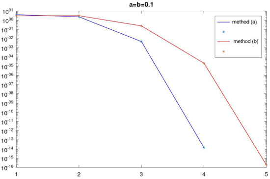
Figure 1. Example 2: norm of correction at each iteration.

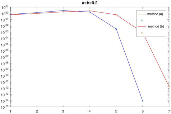
Figure 2. Example 2: norm of correction at each iteration.

The number of iterations of the method (2) differs little for the considered function $B(s)$. However, the following differences can be noted. Method (2)-(a) converges no slower than method (2)-(b); however, the computational complexity of one iteration is higher by $O(n^3)$ operations. Starting from a certain iteration, the correction rate of the method (2)-(a) decreases faster than for the method (2)-(b). In addition, the study of the considered method on different examples showed that it is advisable to choose parameters a and b close to zero. In this case, method (2) converges for a larger number of initial approximations.

Example 3.

Consider the boundary value problem

$$\left\{\begin{array}{c}{\displaystyle y^{″}(t)-y^{\prime }(t)tg(t)+\frac{2y^2(t)}{sin(t)}=0,0<t<\frac{\pi }{2},}\hfill \\ y(0)=0,y(\pi /2)=1.\hfill \end{array}\right.$$

One of the exact solutions is $y_{*}(t)=sin(t)$. Denote ${\upsilon }_i\approx y(t_i)$, $i=0,\dots ,n+1$, where $t_i=ih$ and ${\displaystyle h=\frac{\pi }{2(n+1)}}$. Using the approximation for the first and second-order derivatives

$${\upsilon }_i^{″}\approx \frac{{\upsilon }_{i-1}-2{\upsilon }_i+{\upsilon }_{i+1}}{h^2},{\upsilon }_i^{″}\approx \frac{{\upsilon }_{i+1}-{\upsilon }_{i-1}}{2h},i=1,\dots ,n,$$

we obtain the following system of the nonlinear equations

$$\begin{array}{ccc}\hfill P_i(x)& =& {\displaystyle -2{\upsilon }_i+{\upsilon }_{i+1}-\frac{h}{2}{\upsilon }_{i+1}tg(t_i)+\frac{2h^2{\upsilon }_i^2}{sin(t_i)}=0,i=1,}\hfill \\ \hfill P_i(x)& =& {\displaystyle {\upsilon }_{i-1}-2{\upsilon }_i+{\upsilon }_{i+1}-\frac{h}{2}({\upsilon }_{i+1}-{\upsilon }_{i-1})tg(t_i)+\frac{2h^2{\upsilon }_i^2}{sin(t_i)}=0,i=2,\dots ,n-1,}\hfill \\ \hfill P_i(x)& =& {\displaystyle {\upsilon }_{i+1}-2{\upsilon }_i+1-\frac{h}{2}(1-{\upsilon }_{i-1})tg(t_i)+\frac{2h^2{\upsilon }_i^2}{sin(t_i)}=0,i=n}\hfill \end{array}$$

with $x={({\upsilon }_1,\dots ,{\upsilon }_n)}^T$. Let $a=b=0.1$, $n=19$ and the initial approximation be $x_{0,i}=sin{t}_i+0.5$, $i=1,\dots ,n$. We use $\parallel F(x_k)\parallel \le {10}^{-10}$ as the stopping criteria for this problem. The norm of residuals at each iteration is presented in Table 1.

Table 1. Results for Example 3.

k	Method 2-(a)	Method 2-(b)
1	7.9038 $\times {10}^{-3}$	2.1947 $\times {10}^{-2}$
2	1.9599 $\times {10}^{-5}$	1.1784 $\times {10}^{-4}$
3	4.5432 $\times {10}^{-13}$	2.0348 $\times {10}^{-8}$
4		3.0205 $\times {10}^{-16}$

5. Conclusions

A new methodology is developed to deal with methods using derivatives not related to divided differences or derivatives in the proof of convergence.

In this article, using this methodology, we positively address concerns limiting the applicability of methods whose convergence is based on the Taylor series. Other limitations such as the lack of information on the uniqueness of a solution and a priori estimates of $\parallel x^{*}-x_k\parallel$ or $\parallel x_{k+1}-x_k\parallel$ are also addressed in this article under weak conditions.

The methodology is demonstrated on Symmetric-Steffensen-type multi-step and derivative-free methods using frozen divided differences. But it can be used on other single- as well as multi-step methods as long as they use linear operators which are invertible.

In our future research we plan to utilize this methodology in other methods [1,2,4,6,7,8,9,10,11,12,13,14,15,16].

References

- Traub, J.F. Iterative Methods for the Solution of Equations; Prentice-Hall: Upper Saddle River, NJ, USA, 1964. [Google Scholar]
- Potra, F.; Pták, V. Nondiscrete Induction and Iterative Processes; Pitman Publishing: Lanham, MD, USA, 1984. [Google Scholar]
- Cordero, A.; Torregrosa, J.R. Variants of Newton’s method using fifth-order quadrature formulas. Appl. Math. Comput. 2007, 190, 686–698. [Google Scholar] [CrossRef]
- Amat, S.; Ezquerro, J.; Hernández, M. On a Steffensen-like method for solving nonlinear equations. Calcolo 2016, 53, 171–188. [Google Scholar] [CrossRef]
- Cordero, A.; Villalba, E.G.; Torregrosa, J.R.; Triguero-Navarro, P. Introducing memory to a family of multi-step multidimensional iterative methods with weight function. Expo. Math. 2023, 42, 398–417. [Google Scholar] [CrossRef]
- Alarcón, V.; Amat, S.; Busquier, S.; López, D. Steffensen’s type method in Banach spaces with applications on boundary-value problems. J. Comput. Appl. Math. 2008, 216, 243–250. [Google Scholar] [CrossRef]
- Amat, S.; Argyros, I.; Busquier, S.; Hernández-Verón, M.; Magreñán, A.; Martínez, E. A multistep Steffensen-type method for solving nonlinear systems of equations. Math. Methods Appl. Sci. 2020, 43, 7518–7536. [Google Scholar] [CrossRef]
- Bhalla, S.; Kumar, S.; Argyros, I.; Behl, R.; Motsa, S. High-order modification of Stefensen’s method for solving system of nonlinear equations. Comput. Appl. Math. 2018, 37, 1913–1940. [Google Scholar] [CrossRef]
- Narang, M.; Bhatia, S.; Alshomrani, A.S.; Kanwar, V. General efficient class of Steffensen type methods with memory for solving systems of nonlinear equations. J. Comput. Appl. Math. 2019, 352, 23–39. [Google Scholar] [CrossRef]
- Chicharro, F.I.; Cordero, A.; Garrido, N.; Torregrosa, J.R. Stability and applicability of iterative methods with memory. J. Math. Chem. 2019, 57, 1282–1300. [Google Scholar] [CrossRef]
- Chun, C.; Neta, B.; Kozdon, J.; Scott, M. Choosing weight functions in iterative methods for simple roots. Appl. Math. Comput. 2014, 227, 788–800. [Google Scholar] [CrossRef]
- George, S. On convergence of regularized modified Newton’s method for nonlinear ill-posed problems. J. Inv. Ill-Posed Probl. 2010, 18, 133–146. [Google Scholar] [CrossRef]
- George, S.; Nair, M.T. An a posteriory parameter choice for simplified regularization of ill-posed problems. Inter. Equat. Oper. Th. 1993, 16, 392–399. [Google Scholar] [CrossRef]
- Kung, H.T.; Traub, J.F. Optimal order of one-point and multi-point iteration. J. Assoc. Comput. Mach. 1974, 21, 643–651. [Google Scholar] [CrossRef]
- Argyros, I.K.; Shakhno, S. Extended local convergence for the combined Newton-Kurchatov method under the generalized Lipschitz conditions. Mathematics 2019, 7, 207. [Google Scholar] [CrossRef]
- Weeracoon, S.; Ferando, T. A variant of Newton’s method with accelerated third-order convergence. Appl. Math. Lett. 2000, 13, 87–93. [Google Scholar] [CrossRef]
Disclaimer/Publisher’s Note: The statements, opinions and data contained in all publications are solely those of the individual author(s) and contributor(s) and not of MDPI and/or the editor(s). MDPI and/or the editor(s) disclaim responsibility for any injury to people or property resulting from any ideas, methods, instructions or products referred to in the content. |
© 2024 by the authors. Licensee MDPI, Basel, Switzerland. This article is an open access article distributed under the terms and conditions of the Creative Commons Attribution (CC BY) license (https://creativecommons.org/licenses/by/4.0/).