Viscous Dissipation and Mixed Convection Effects on the Induced Magnetic Field for Peristaltic Flow of a Jeffrey Nanofluid

Abstract

The issue of Jeffrey nanofluid peristaltic flow in an asymmetric channel being affected by an induced magnetic field was studied. In addition, mixed convection and viscous dissipation were considered. Under the supposition of a long wave length and a low Reynolds number, the problem was made simpler. The system and corresponding boundary conditions were solved numerically by using the built-in package NDSolve in Mathematica software. This software ensures that the boundary value problem solution is accurate when the step size is set appropriately. It computes internally using the shooting method. Axial velocity, temperature distribution, nanoparticle concentration, axial induced magnetic field, and density distribution were all calculated numerically. An analysis was conducted using graphics to show how different factors affect the flow quantities of interest. The results showed that when the Jeffrey fluid parameter is increased, the magnitude of axial velocity increases at the upper wall of the channel, while it decreases close to the lower walls. Increasing the Hartmann number lads to increases in the axial velocity near the channel walls and in the concentration of nanoparticles. Additionally, as the Brownian motion parameter is increased, both temperature and nanoparticle concentration grow.

1. Introduction

Peristaltic flows are flow patterns in tubes or channels that are caused by the walls of an oscillating channel. Peristaltic flows are widely observed in physiology and engineering. This is because of all the practical uses they have, such as when food is swallowed through the esophagus, when lymph is transported in lymphatic vessels, when the ureter transports urine from the kidney to the bladder, when chyme and ovaries are moved through the gastrointestinal tract, when eggs are moved through the fallopian tube, when blood pumps are used in heart–lung machines, when toxic fluid is transported through the peristaltic method in the nuclear industry, etc.

A fluid is called a nanofluid if it contains particles smaller than one nanometer. These fluids are composed of nanoparticles in engineered colloidal suspensions inside a base fluid. The most popular materials for the nanoparticles used in nanofluids include metals, oxides, carbides, or carbon nanotubes. Water, oil, and ethylene glycol are the basic fluids. Nanofluids have unique features that might make them beneficial for a range of uses, including heat transfer, fuel cells, medicine, and hybrid engines. They have been extensively employed in engineering equipment for engine cooling and vehicle thermal management, as well as for home refrigerators, chillers, heat exchangers, and nuclear reactors. Additionally, they are quite stable and do not have any additional issues like erosion, sedimentation, higher pressure drops, etc.

The study of MHD examines how highly conductive fluids move when a magnetic field is present. The MHD flow of nanofluids in a channel with peristalsis is of relevance regarding many difficulties related to the movement of conductive physiological nanofluids. For example, hemoglobin, intercellular protein, and cell membranes combine to make blood a biomagnetic fluid. Hydromagnetic peristaltic flow has applications in the fields of magnetic resonance imaging (MRI), magnetic devices, and in magnetic particles employed as drug carriers. Mekheimer [1,2] investigated how an induced magnetic field affected the conducting, coupled magneto–micropolar stress of a fluid under peristaltic flow. Hayat et al. [3] spoke about the effect of an induced magnetic field on the peristaltic transport of a third-order fluid. Hayat et al. have also investigated how an induced magnetic field affects a Carreau fluid’s peristaltic flow [4]. The effect of induced magnetic field on the peristaltic flow in an annulus was further studied by Abd Elmaboud [5]. In the presence of an induced magnetic field, the peristaltic flow of a Williamson fluid was solved analytically and numerically by Akram et al. [6]. The effects of an induced magnetic field and heat transfer on the peristaltic flow of a Jeffrey fluid were examined by Akram and Nadeem [7]. Using a vertical channel, Mustafa et al. [8] examined how an induced magnetic field affected the mixed convection peristaltic flow of nanofluid. In a channel with wall characteristics, Hayat et al. [9] address the magnetohydrodynamic peristaltic motion of nanofluid. Theoretical model for the modern drug delivery system by taking Hall and Joule heating into account is developed by Abbasi et al. [10]. The influence of radiation and a magnetic field on the peristaltic transport of nanofluids via a porous area in a tapered asymmetric channel was theoretically examined by Kothandapani and Prakash [11]. Hall effects in a curved channel were used by Abbasi et al. [12] to analyze the effects of magnetic field on the peristalsis of Carreau-Yasuda fluid. In an inclined channel under convective circumstances, Hayat et al. [13] studied the impact of an inclined magnetic field on the peristaltic flow of Williamson fluid. Hayat et al. [14] studied the Soret and Dufour influences on peristaltic motion with a radial magnetic field and convective circumstances in a curved channel. The effect of a magnetic field on Sisko nanofluid flow in three dimensions under convective conditions was studied by Hayat et al. [15]. In their study on the peristaltic transport of a Jeffrey nanofluid with Joule heating, Hayat et al. [16] looked at the effects of Hall and ion slip. Nowar [17] addressed the closed-form solution to study the impact of an induced magnetic field on the peristaltic transport of a nanofluid in an asymmetric channel. Recently, Kavya et al. [18] investigated the changing properties of a laminar, stable, incompressible, two-dimensional, non-Newtonian pseudoplastic Williamson hybrid nanofluid along a stretched cylinder in terms of both fluid momentum and thermal energy.

A Jeffrey fluid is a non-Newtonian viscoelastic fluid model that effectively illustrates retardation and relaxation times. Jeffrey nanofluids have several practical applications in various fields, for example, heat transfer enhancement due to their enhanced thermal conductivity; biomedical applications, particularly in drug delivery and hyperthermia treatment for cancer; energy storage; lubrication and friction reduction. By adding Jeffrey nanofluids to lubricants, it can improve their lubricating properties and reduce friction in various mechanical systems. The transformation of mechanical energy into heat as a result of internal friction in a moving fluid is known as viscous dissipation. In the case of peristaltic flow of a Jeffrey nanofluid under the influence of an induced magnetic field, viscous dissipation plays a role in the energy balance of the system. Mixed convection can enhance or suppress heat transfer rates depending on the relative strengths of the natural and forced convection components.

It has been noted that the peristaltic flows of nanofluids with an induced magnetic field have not gained much attention, despite several attempts by researchers to study MHD peristaltic transport in the presence of a uniform magnetic field. With these reasons in mind, the current study’s objective was to look at how an induced magnetic field affects the peristaltic flow of a Jeffrey nanofluid inside an asymmetric channel that has both mixed convection and viscous dissipation. In summary, understanding the importance of viscous dissipation and mixed convection effects in the induced magnetic field peristaltic flow of a Jeffrey nanofluid is crucial for predicting and optimizing the behavior of the fluid in various applications. Graphs of the data are displayed for evaluating the impacts of pertinent variables on temperature, axially induced magnetic field, nanoparticle concentration, velocity, and current density distribution. For more generality, in case of 2D or 3D geometries, we can use the lattice Boltzmann method [19,20] as an alternative method to solve the obtained system of partial differential equations.

2. Problem Formulation

Our goal was to analyze the peristaltic motion of a Jeffrey nanofluid that is incompressible and viscous and electrically conducts in a two-dimensional, infinitely asymmetric channel of width $d_1+d_2$. Assuming sinusoidal wave trains traveling along the channel walls, as depicted in Figure 1, with constant speed c cause asymmetry in the channel. As opposed to the top wall, which is kept at temperature $T_0$ and nanoparticle concentration $C_0$, the bottom wall of the channel is kept at $T_1$ and $C_1$. The channel walls’ forms are displayed in the following equations:

$$H_1(X,t)=d_1+a_{1}cos\left[\frac{2\pi }{\lambda }(X-ct)\right],\mathrm{at}\mathrm{upper}\mathrm{wall}$$

(1)

$$H_2(X,t)=-d_2-a_{2}cos[\frac{2\pi }{\lambda }(X-ct)+\varphi ],\mathrm{at}\mathrm{lower}\mathrm{wall}$$

(2)

where $a_1$ and $a_2$ are the amplitudes of the top and bottom waves, the wave length is $\lambda$, c is the propagation velocity, the time is denoted by t, X is the wave propagation direction, $\varphi$ is the difference of phase, and its range is $0\le \varphi \le \pi$. Keep in mind that $\varphi =0$ characterizes an asymmetric channel with out-of-phase waves, whereas $\varphi =\pi$ illustrates the situation when waves are in-phase. Additionally, $d_1$, $d_2$, $a_1$, $a_2$, and $\varphi$ fulfill the inequality below.

$$a_1^2+a_2^2+2a_1{a}_{2}cos\varphi \le {(d_1+d_2)}^2$$

(3)

in order to prevent intersections between the walls.

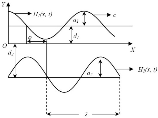
Figure 1. The problem’s geometry.

With X running parallel to the channel’s center line and Y running transverse to it, we adopt a Cartesian coordinate system for the channel. An induced magnetic field $\mathbf{H}(h_x(X,Y,t),h_Y(X,Y,t),0)$ is produced when a magnetic field of constant intensity $H_0$ acts transversely. Thus, the whole magnetic field is ${\mathbf{H}}^{+}(h_x(X,Y,t),H_0+h_Y(X,Y,t),0)$. The velocity field is denoted by $\mathbf{V}=\left(U\right(X,Y,t),V(X,Y,t),0)$, where U and V stand for the X and Y directions and U and V, respectively. The following equation converts the laboratory frame of reference $(X,Y)$ to the wave frame of reference $(x,y)$

$$x=X-ct,y=Y,u=U-c,v=V,\mathrm{and}p\left(x\right)=P(x,t)$$

(4)

where $(u,v)$, p and $(U,V)$, P are, respectively, the velocity and pressure components in the wave and fixed frames of reference.

The expression of Cauchy stress tensor $\tau$ for Jeffrey fluid is given by the following equation:

$$\tau =-p\mathbf{I}+\mathbf{S},\mathbf{S}=\frac{\mu }{1+{\lambda }_1}\left(\dot{\gamma }+{\lambda }_2\frac{d\dot{\gamma }}{dt}\right),\dot{\gamma }=\nabla \mathbf{V}+{(\nabla \mathbf{V})}^T$$

(5)

Here, $\mathbf{S}$ stands for extra-stress tensor, ${\lambda }_1$ is a measure of the relaxation-to-retardationt-times ratio, ${\lambda }_2$ is the retardation time, p is the pressure, $\mathbf{I}$ is the identity tensor, $\mu$ is the viscosity coefficient, $\dot{\gamma }$ is the shear rate, $\mathbf{V}$ is the velocity vector, and $\frac{d}{dt}$ is the substantial derivative.

For the current flow, the governing equations of motion are (see [2,8,9,17]) as follows:

(I) The Maxwell’s equations are

$$\nabla .\mathbf{H}=0,\nabla .\mathbf{E}=0$$

(6)

$$\nabla \times \mathbf{H}=\mathbf{J},\mathbf{J}=\sigma [\mathbf{E}+{\mu }_e(\mathbf{V}\times \mathbf{H})]$$

(7)

$$\nabla \times \mathbf{E}=-{\mu }_e\frac{\partial \mathbf{H}}{\partial t}$$

(8)

(II) The continuity equation is

$$\nabla .\mathbf{V}=0$$

(9)

(III) The momentum equation is

$${\rho }_f\frac{d\mathbf{V}}{dt}=-\nabla \mathbf{P}+div\mathbf{S}-{\mu }_e({\mathbf{H}}^{+}.\nabla ){\mathbf{H}}^{+}-\frac{{\mu }_e}{2}\nabla {\mathbf{H}}^{+2}+$$

$$(1-C_0){\rho }_{f}g\alpha (T-T_0)+({\rho }_p-{\rho }_f)g\beta (C-C_0)$$

(10)

(IV) The equation of nanofluid temperature is

$${\left(\rho c^{\prime }\right)}_f\frac{dT}{dt}=k{\nabla }^{2}T+{\left(\rho c^{\prime }\right)}_p[D_B\nabla C\nabla T+(D_T/T_0)\nabla T\nabla T]+\mathbf{S}.\mathbf{L}$$

(11)

(V) The nanoparticle volume fraction phenomena equation is

$$\frac{dC}{dt}=D_B{\nabla }^{2}C+(D_T/T_0){\nabla }^{2}T$$

(12)

(VI) The induction equation is

$$\frac{\partial {\mathbf{H}}^{+}}{\partial t}=\nabla \times (V\times {\mathbf{H}}^{+})+\frac{1}{\zeta }{\nabla }^2{\mathbf{H}}^{+}$$

(13)

where E is the strength of the electric field, $\mathbf{L}=\nabla \mathbf{V}$, ${\mu }_e$ is the permeability of magnetism, ${\rho }_f$ is the fluid density, ${\nabla }^2$ is the Laplacian operator, t is time, ${\left(\rho c^{\prime }\right)}_f$ is the base fluid’s heat capacity, ${\left(\rho c^{\prime }\right)}_p$ is the particle material’s intrinsic heat capacity, $c^{\prime }$ is the coefficient of the volumetric volume expansion, C is the volume fraction of nanoparticles, T is the dimensional temperature of the nanofluid, $D_B$ is the coefficient of Brownian diffusion, $D_T$ is the coefficient of the thermophoretic diffusion, and $\zeta$ is the inverse of magnetic diffusivity. To describe the fluid flow in a nondimensional form, we define the following quantities [16]:

$$\begin{array}{c}{x}^{*}=\frac{x}{\lambda },y^{*}=\frac{y}{d_1},u^{*}=\frac{u}{c},v^{*}=\frac{v}{c},h_1=\frac{H_1}{d_1},h_2=\frac{H_2}{d_1},\delta =\frac{d_1}{\lambda },R_e=\frac{{\rho }_f{d}_{1}c}{\mu },t^{*}=\frac{c}{\lambda }t,\hfill \\ \nu =\frac{\mu }{{\rho }_f},p^{*}=\frac{p{d}_1^2}{c\lambda \mu },b=\frac{a_2}{d_1},d=\frac{d_2}{d_1},a=\frac{a_1}{d_1},\alpha =\frac{k}{{\left(\rho c^{\prime }\right)}_f},\theta =\frac{T-T_0}{T_1-T_0},\Omega =\frac{C-C_0}{C_1-C_0},\\ N_b=\frac{\rho c_p^{\prime }{D}_B(c_1-c_0)}{{\left(\rho c^{\prime }\right)}_f\alpha },N_t=\frac{\rho c_p^{\prime }{D}_T(T_1-T_0)}{{\left(\rho c\right)}_f\alpha T_0},Gr=\frac{\alpha g(T_1-T_0)d_1^2}{\nu c},S=\frac{H_0}{C}\sqrt{{\mu }_e/{\rho }_f},\\ \hfill Qr=\frac{\alpha g(C_1-C_0)d_1^2}{\nu c},Pr=\frac{\nu }{\alpha },\Phi =\frac{\Phi }{H_0{d}_1},p_m=p+\frac{1}{2}{R}_e\delta \frac{{\mu }_e{H}^{+2}}{{\rho }_f{c}^2},R_m=\sigma {\mu }_{e}c{d}_1,\end{array}$$

$$h_X={\Phi }_Y,h_Y=-{\Phi }_X,S_{ij}=\frac{d_1}{\mu c}{S}_{ij}^{*},Ec=\frac{c^2}{c_f(T_1-T_0)}$$

(14)

where $\delta$ is the dimensionless wave number, $R_e$ is the Reynolds number, $\nu$ is the dynamic viscosity parameter, $\alpha$ is a thermal expansion parameter, $N_b$ is the Brownian motion parameter, $N_t$ is the thermophoresis parameter, $Gr$ is the local temperature Grashof number, S is Stommer’s number, $Qr$ is the local nanoparticle Grashof number, $Pr$ is the Prandtl number, $R_m$ is the magnetic Reynolds number, and $Ec$ is the Eckert number.

After entering Equations (4) and (14) into Equations (9) to (13), we obtain

$$\delta \frac{\partial u}{\partial x}+\frac{\partial v}{\partial x}=0$$

(15)

$$\delta R_{e}u\frac{\partial u}{\partial x}+R_{e}v\frac{\partial u}{\partial y}=-\frac{\partial p_m}{\partial x}+\delta \frac{\partial S_{xx}}{\partial x}+\frac{\partial S_{xy}}{\partial y}+\delta R_e{S}^2({\Phi }_y\frac{\partial {\Phi }_y}{\partial x}-{\Phi }_x\frac{\partial {\Phi }_y}{\partial y})$$

$$+R_e{S}^2\frac{\partial {\Phi }_y}{\partial y}+Gr\Theta +Qr\Omega$$

(16)

$${\delta }^2{R}_{e}u\frac{\partial v}{\partial x}+\delta R_{e}v\frac{\partial v}{\partial y}=-\frac{\partial p_m}{\partial y}+{\delta }^2\frac{\partial S_{xy}}{\partial x}+\delta \frac{\partial S_{yy}}{\partial y}-$$

$${\delta }^3{R}_e{S}^2({\Phi }_y\frac{\partial {\Phi }_x}{\partial x}-{\Phi }_x\frac{\partial {\Phi }_x}{\partial y})-{\delta }^2{R}_e{S}^2\frac{{\partial }^2\Phi }{\partial x\partial y}$$

(17)

$$R_{e}Pr(\delta u\frac{\partial \theta }{\partial x}+v\frac{\partial \theta }{\partial y})={\delta }^2\frac{{\partial }^2\theta }{\partial x^2}+\frac{{\partial }^2\theta }{\partial y^2}+N_b({\delta }^2\frac{\partial \Omega }{\partial x}\frac{\partial \theta }{\partial x}+\frac{\partial \Omega }{\partial y}\frac{\partial \theta }{\partial y})+N_t({\delta }^2{\left(\frac{\partial \theta }{\partial x}\right)}^2+{\left(\frac{\partial \theta }{\partial y}\right)}^2)+$$

$$Br[\delta S_{xx}\frac{\partial u}{\partial x}+S_{xy}(\frac{\partial u}{\partial y}+\delta \frac{\partial v}{\partial x})+S_{yy}\frac{\partial v}{\partial y}]$$

(18)

$$\frac{\delta c\lambda }{D_B}(\delta \frac{\partial \Omega }{\partial x}+\frac{\partial \Omega }{\partial y})={\delta }^2\frac{{\partial }^2\Omega }{\partial x^2}+\frac{{\partial }^2\Omega }{\partial y^2}+\frac{N_b}{N_t}({\delta }^2\frac{{\partial }^2\theta }{\partial x^2}+\frac{{\partial }^2\theta }{\partial y^2})$$

(19)

$$E=u-\delta u\frac{\partial \Phi }{\partial x}-v\frac{\partial \Phi }{\partial y}+\frac{1}{R_m}(\frac{{\partial }^2\varphi }{\partial y^2}+{\delta }^2\frac{{\partial }^2\varphi }{\partial x^2})$$

(20)

where,

$$S_{xx}=\frac{2\delta }{1+{\lambda }_1}[1+{\lambda }_2^{*}(\delta u\frac{\partial }{\partial x}-v\frac{\partial }{\partial y})]\frac{\partial u}{\partial x}$$

(21)

$$S_{xy}=\frac{1}{1+{\lambda }_1}[1+{\lambda }_2^{*}(\delta u\frac{\partial }{\partial x}-v\frac{\partial }{\partial y})](\frac{\partial u}{\partial y}-\delta \frac{\partial v}{\partial x})$$

(22)

$$S_{yy}=\frac{2\delta }{1+{\lambda }_1}[1+{\lambda }_2^{*}(\delta u\frac{\partial }{\partial x}-v\frac{\partial }{\partial y})]\frac{\partial u}{\partial x}.$$

(23)

Under the assumptions of a long wavelength and a low Reynolds number and after the stars are dropped, the dimensionless form of the flow equations for this model in terms of the stream function $\psi (x,y)$ (considering $u=\partial \psi /\partial y$ and $v=-\delta \partial \psi /\partial x$) produce the following equations:

$$\frac{\partial p_m}{\partial x}=\frac{\partial S_{xy}}{\partial y}+R_e{S}^2\frac{{\partial }^2\Phi }{\partial y^2}+Gr\theta +Qr\Omega$$

(24)

$$\frac{\partial p_m}{\partial y}=0$$

(25)

$$\frac{{\partial }^2\theta }{\partial y^2}+N_b\frac{\partial \theta }{\partial y}\frac{\partial \Omega }{\partial y}+N_t{\left(\frac{\partial \theta }{\partial y}\right)}^2+Br{S}_{xy}\frac{{\partial }^2\Psi }{\partial y^2}=0$$

(26)

$$\frac{{\partial }^2\Omega }{\partial y^2}+\frac{N_t}{N_b}\frac{{\partial }^2\theta }{\partial y^2}=0$$

(27)

$$E=\frac{\partial \psi }{\partial y}+\frac{1}{R_m}\frac{{\partial }^2\Phi }{\partial y^2}.$$

(28)

Using Equations (22) and (28) in Equation (24) and eliminating the pressure between Equations (24) and (25), we have

$$\frac{1}{1+{\lambda }_1}\frac{{\partial }^4\psi }{\partial y^4}-M^2\frac{{\partial }^2\psi }{\partial y^2}+Gr\frac{\partial \theta }{\partial y}+Qr\frac{\partial \Omega }{\partial y}=0,$$

(29)

$$\frac{{\partial }^2\theta }{\partial y^2}+N_b\frac{\partial \theta }{\partial y}\frac{\partial \Omega }{\partial y}+N_t{\left(\frac{\partial \theta }{\partial y}\right)}^2+\frac{Br}{1+{\lambda }_1}{\left(\frac{{\partial }^2\psi }{\partial y^2}\right)}^2=0,$$

(30)

where $M^2=R_e{S}^2{R}_m$ is the Hartmann number, and $Br=PrEc$ is the Brinkman number. The corresponding boundary conditions are given by the following equations:

$$\psi =\frac{F}{2},\frac{\partial \psi }{\partial y}=-1,\theta =0,\Omega =0,\Phi =0,\mathrm{at}y=h_1\left(x\right)=1+acos2\pi x$$

(31)

$$\psi =-\frac{F}{2},\frac{\partial \psi }{\partial y}=-1,\theta =1,\Omega =1,\Phi =0,\mathrm{at}y=h_2\left(x\right)=-d-bcos(2\pi x+\varphi )$$

(32)

where F is the flux in the wave frame; a, b, $\varphi$, and d satisfy the following inequality

$$a^2+b^2+2abcos\varphi \le (1+d^2).$$

3. Numerical Solutions and Discussion

We now investigate the effects of physical quantities on axial velocity, temperature distribution, nanoparticles’ concentration distribution, axial-induced magnetic field, and current density distribution.

3.1. Validation of the Model

The above-mentioned nonlinear Equations (27) to (30), subject to boundary conditions expressed by Equations (31) and (32), are extremely challenging to handle analytically. Hence, we computed the graphical solutions by using the built-in package NDSolve in Mathematica software. This software ensures that the boundary value problem solution is accurate when the step size is set appropriately. It computes internally using the shooting method technique. In the shooting method, the PDE is transformed into a system of ordinary differential equations (ODEs) by considering the spatial variables as parameters. This allowed us to solve the problem as an initial value problem (IVP) rather than as a boundary value problem (BVP). The shooting method is an iterative process that requires adjusting the initial guess until the desired accuracy is achieved. It is widely used in various fields of science and engineering to solve nonlinear PDEs, such as in fluid dynamics, heat transfer, and quantum mechanics. The obtained results are in very good agreement with those in [7,8,16] (see Table 1).

Table 1. Comparison of velocity profile from this study with that of a previously published article.

y	Current Study	Akram et al. [7]
−1	0.48996	0.03
−0.5	1.32663	0.6
0	1.49879	0.8
0.5	1.3595	0.82
1	0.842943	0.72

Note that the velocity profile in both studies has the same parabola shape. The variations in velocity values result from the usage of different values for other factors. The subsequent subsections deal with plots of velocity u, temperature distribution function $\Theta$, nanoparticle concentration distribution function $\Omega$, axial-induced magnetic field $h_x$, and current density distribution $J_z$.

3.2. Axial Velocity Profile

Axial velocity is shown in Figure 2 in relation to the Hartmann number M, the local temperature Grashof number $Gr$, the local nanoparticles’ Grashof number $Qr$, and the Jeffrey fluid parameter ${\lambda }_1$. According to Figure 2a, the velocity field’s magnitude rises close to the channel wall, while it reduces in the middle of the channel and is the largest for low values of M there. Physically, this result is consistent with the well-known Hartmann result that states “increasing the magnetic field strength causes a decay in the velocity”. As seen in Figure 2b, when $Gr$ rises, the magnitude of velocity rises in the center of the channel, where buoyant forces resulting from the temperature gradient exceed the viscous forces, while it leads to a decrease in velocity near the channel’s walls, where viscous forces are dominant. Figure 2c demonstrates that the velocity rises as $Qr$ grows at the lower wall side and falls as $Qr$ increases at the higher wall side. Figure 2d shows the impact of the Jeffrey fluid parameter ${\lambda }_1$ on axial velocity. The relaxation-to-retardation-time ratio for a Jeffrey fluid is ${\lambda }_1$. Fluids with a significant relaxation time distinguishe them as viscoelastic fluids. It appears that the velocity rises in a region closed to the lower wall and decreases in another region closer to the higher wall with an increase in ${\lambda }_1$. In actuality, when ${\lambda }_1$ is increased, the flow resistance reduces in the bottom portion of the channel owing to the short retardation time and increases in the top section of the channel due to the long retardation time. It indicates that it takes a lot longer for fluid particles to return from a disturbed system to an equilibrium system. As a result, the fluid’s velocity drops.

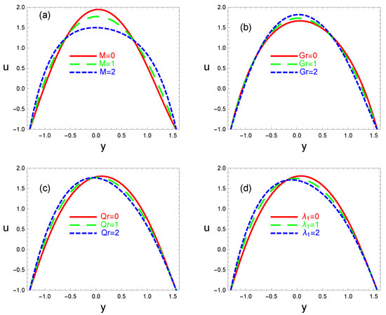
Figure 2. Variations in velocity profile $\mathrm{u}$ with $\mathrm{y}$ for various values of Hartmann number M (a), local Grashof number $Gr$ (b), nanoparticles’ Grashof number $Qr$ (c), and Jeffrey fluid parameter ${\lambda }_1$ (d). The other parameters chosen are $F=2.5,x=0.1,d=2,a=0.7,$ $b=1.2,$ $N_b=0.8,N_t=0.4,\varphi =\frac{\pi }{2},Gr=1.5,Br=1.7,E=1,{\lambda }_1=0.5,Qr=1,R_m=4$ (panel a); $F=2.5,x=0.1,d=2,a=0.7,b=1.2,N_b=0.8,N_t=0.4,\varphi =\frac{\pi }{2},M=1,Br=1.7,$ $E=1,$ ${\lambda }_1=0.5,Qr=1,R_m=4$ (panel b); $F=2.5,x=0.1,d=2,$ $a=0.7,b=1.2,N_b=0.8,N_t=0.4,$ $\varphi =\frac{\pi }{2},Gr=1.5,Br=1.7,E=1,{\lambda }_1=0.5,M=1,R_m=4$ (panel c); $F=2.5,x=0.1,d=2,$ $a=0.7,$ $b=1.2,N_b=0.8,N_t=0.4,\varphi =\frac{\pi }{2},Gr=1.5,Br=1.7,E=1,M=1,Qr=1,R_m=4$ (d).

3.3. Temperature Distribution Profile

Figure 3 shows the influences of Hartmann number M, thermophoresis parameter $N_t$, Brownian motion parameter $N_b$, and local temperature Grashof number $Gr$ on the temperature distribution profile. It is obvious from Figure 3a that temperature decreases by increasing the magnitude of M. Physically, magnetic force acts as a retarding force, and so it slows down the motion of fluid particles. As a result, the kinetic energy decreases, and thus temperature decreases. Figure 3b,c show opposite behaviors of $N_t$ and $N_b$. We see that temperature decreases with an increase in $N_t$ and increases if $N_b$ is increased. Increasing $N_b$ leads to increased the kinetic energy of the nanoparticles and transforms it into internal energy that raises the nanofluid temperature. However, when $N_t$ increases, more nanoparticles migrate from hot to cold locations inside the nanofluid, lowering the temperature of the nanofluid. The fact that thermophoresis operates against a temperature gradient is obviously supported by this result. The effect of $Gr$ on temperature profile is considered in Figure 3d. It is obvious that when $Gr$ rises, the temperature rises as well. This is because increasing the Grashof number causes the buoyant forces to increase, which in turn increases temperature and fluid flow.

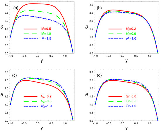
Figure 3. Variations in a fluid’s local temperature $\theta$ with respect to $\mathrm{y}$ for different values of the Hartmann number M, thermophoresis parameter $N_t$, Brownian motion parameter $N_b$, and local temperature Grashof number $Gr$ are shown in panels a through d. The other factors considered are $F=3.5,x=1,d=1,a=0.3,b=0.7,N_b=0.8,N_t=0.4,\varphi =\frac{\pi }{2},Gr=1,Br=2,E=2,{\lambda }_1=3,$ $Qr=1,R_m=4$ (panel a); $F=3.5,x=1,d=1,a=0.3,b=0.7,N_b=0.8,M=1,\varphi =\frac{\pi }{2},$ $Gr=1,Br=2,E=2,{\lambda }_1=3,Qr=1,R_m=4$ (panel b); $F=3.5,x=1,d=1,a=0.3,b=0.7,M=1,$ $N_t=0.4,\varphi =\frac{\pi }{2},Gr=1,Br=2,E=2,{\lambda }_1=3,Qr=1,R_m=4$ (panel c); $F=3.5,x=1,d=1,$ $a=0.3,$ $b=0.7,N_b=0.8,N_t=0.4,\varphi =\frac{\pi }{2},M=1,Br=2,E=2,{\lambda }_1=3,Qr=1,R_m=4$ (d).

3.4. Nanoparticle Concentration Distribution Profile

Figure 4 illustrates the effects of the Hartmann number M, Brownian motion parameter $N_b$, thermophoresis parameter $N_t$, and local temperature Grashof number $Gr$ on the distribution profile of nanoparticle concentration. It is evident from Figure 4a that the distribution of nanoparticle concentrations rises as M rises. Figure 4b,c reveal that the nanoparticle concentration profile is an increasing function of $N_b$ and is a decreasing function of $N_t$. Actually, the particles in a fluid are always moving due to Brownian motion. As a result, particles are kept from settling and colloidal solutions remain stable and, hence, the nanoparticle concentration increases as the Brownian motion parameter increases. According to Figure 4d, the distribution of nanoparticle concentrations diminishes as $Gr$ increases. This is because the buoyancy force due to spatial variation in fluid density (generated by the temperature gradient) becomes more dominant than to the retarding (viscous) force caused by viscosity force.

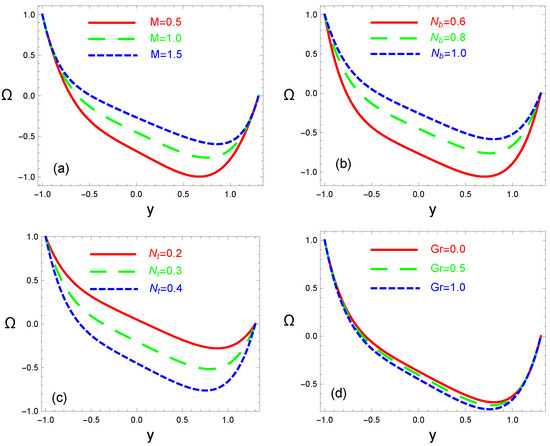
Figure 4. Variations in nanoparticle concentration $\Omega$ with $\mathrm{y}$ for various values of Hartmann number M (a), Brownian motion parameter $N_b$ (b), thermophoresis parameter $N_t$ (c), and local temperature Grashof number $Gr$ (d). The other parameters chosen are $F=3.5,x=1,$ $d=1,a=0.3,b=0.7,N_b=0.8,N_t=0.4,\varphi =\frac{\pi }{2},Gr=1,Br=2,E=2,{\lambda }_1=3,Qr=1,R_m=4$ (panel a); $F=3.5,x=1,d=1,a=0.3,b=0.7,M=1,N_t=0.4,\varphi =\frac{\pi }{2},Gr=1,Br=2,$ $E=2,{\lambda }_1=3,Qr=1,R_m=4$ (panel b); $F=3.5,x=1,d=1,a=0.3,b=0.7,N_b=0.8,M=1,$ $\varphi =\frac{\pi }{2},Gr=1,Br=2,E=2,{\lambda }_1=3,Qr=1,R_m=4$ (panel c); $F=3.5,x=1,d=1,a=0.3,b=0.7,$ $N_b=0.8,N_t=0.4,\varphi =\frac{\pi }{2},M=1,Br=2,E=2,{\lambda }_1=3,Qr=1,R_m=4$ (panel d).

3.5. Axially Induced Magnetic Field Profile

The magnetic field created along the direction of fluid flow as a result of the movement of the nanofluid and the presence of an applied magnetic field is referred to as the axially induced magnetic field. The relationships between the axially induced magnetic field $h_x$ and the Hartmann number M, Jeffrey fluid parameter ${\lambda }_1$, magnetic Reynolds number $R_m$, and electric field intensity E are shown in Figure 5. It is clear that the profiles of $h_x$ have one direction in the half-region $(y>0)$ and an opposite direction in the other half $(y<0)$. Additionally, we notice that $h_x$ is symmetric about the channel and that it decreases in the channel’s lower half and increases in the top half as M, ${\lambda }_1$, and E rise (see Figure 5a,b,d). Physical interpretations imply that either the fluid is more sensitive to the applied magnetic field or that the fluid’s nanoparticles have stronger magnetic characteristics in the channel’s upper half. On the other hand, when $R_m$ rises, $h_x$ increases (see Figure 5c). In the world of physics, as $R_m$ grows, magnetic permeability also rises, which results in a rise in the induced magnetic field.

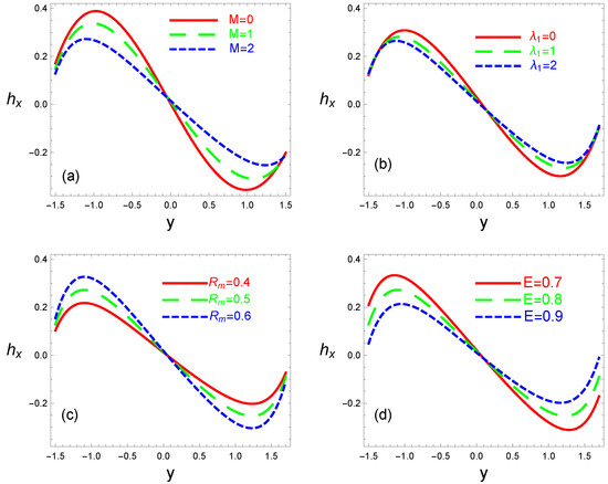
Figure 5. Variations in axial induced magnetic field $h_x$ against space variable y for different values of Hartmann number M (panel a), Jeffrey fluid parameter ${\lambda }_1$ (panel b), magnetic Reynolds number $R_m$ (panel c), and electric field intensity E (panel d). The other parameters chosen are $F=3,x=0,$ $d=2.2,a=0.7,b=0.7,N_b=0.8,$ $N_t=0.4,\varphi =\pi ,Gr=0.5,Br=0.7,E=0.8,{\lambda }_1=1.5,Qr=0.6,$ $R_m=0.5$ (panel a); $F=3,x=0,d=2.2,a=0.7,b=0.7,N_b=0.8,$ $N_t=0.4,\varphi =\pi ,Gr=0.5,$ $Br=0.7,$ $E=0.8,M=2,Qr=0.6,R_m=0.5$ (panel b); $F=3,x=0,d=2.2,a=0.7,$ $b=0.7,$ $N_b=0.8,$ $N_t=0.4,\varphi =\pi ,Gr=0.5,Br=0.7,E=0.8,{\lambda }_1=1.5,Qr=0.6,M=2$ (panel c); $F=3,x=0,d=2.2,$ $a=0.7,b=0.7,N_b=0.8,N_t=0.4,\varphi =\pi ,Gr=0.5,Br=0.7,M=2,$ ${\lambda }_1=1.5,Qr=0.6,R_m=0.5$ (panel d).

3.6. Current Density Distribution Profile

Figure 6 illustrates the current density distribution function $J_z$ versus the space variable y for various Hartmann numbers, Jeffrey fluid parameters, magnetic Reynolds numbers, and electric field intensities. Current density distribution refers to the spatial variations in current density within a conductive material or medium. Current density is a measure of the flow of electric charge per unit area and is expressed in amperes per square meter $(A/m^2)$ in an SI system. In general, the physical significance of current density distribution is that it offers crucial details on the movement of electric charges across various materials. Figure 6a,b show that $J_z$ grows near the channel walls and decreases in the channel middle as M and ${\lambda }_1$ increase. In Figure 6a, raising M results in lower fluid flow rates and temperatures, and a drop in temperature enhances the possibility of raising the thermal insulation, which lowers the current density distribution. In Figure 6b, as ${\lambda }_1$ is increased, the velocity distribution declines due to the rise in the boundary layer momentum thickness in the middle of the channel, which in turn causes the current density distribution to drop. A rise in $R_m$ fundamentally changes the situation, as shown in Figure 6c. The rationale for this is because stronger currents are frequently associated with greater $R_m$ values. This suggests that the magnetic field’s advection is more important than its diffusion. Figure 6d shows that $J_z$ is a decreasing function of E. This is because an electric field causes the suspended nanoparticles in the nanofluid to align themselves, which raises the viscosity of the fluid. Variations in viscosity can modify the fluid motion’s efficiency, which can have an indirect impact on the current density’s distribution.

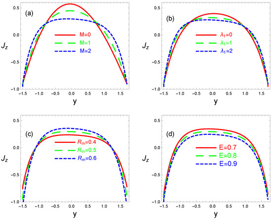
Figure 6. Variations in the current density distribution $J_z$ within y for different values of Hartmann number M (panel a), Jeffrey fluid parameter ${\lambda }_1$ (panel b), magnetic Reynolds number $R_m$ (panel c), and electric field intensity E (panel d). The other parameters chosen are $F=3,x=0,d=2.2,$ $a=0.7,b=0.7,N_b=0.8, N_t=0.4,\varphi =\pi ,Gr=0.5,Br=0.7,E=0.8,{\lambda }_1=1.5,Qr=0.6,R_m=0.5$ (panel a); $F=3,x=0,d=2.2,a=0.7,b=0.7,N_b=0.8,$ $N_t=0.4,\varphi =\pi ,Gr=0.5,Br=0.7,$ $E=0.8,$ $M=2,Qr=0.6,R_m=0.5$ (panel b); $F=3,x=0,d=2.2,a=0.7,b=0.7,N_b=0.8,$ $N_t=0.4,$ $\varphi =\pi ,Gr=0.5,Br=0.7,$ $E=0.8,{\lambda }_1=1.5,Qr=0.6,M=2$ (panel c); $F=3,x=0,d=2.2,$ $a=0.7,b=0.7,N_b=0.8,N_t=0.4,\varphi =\pi ,Gr=0.5,Br=0.7,M=2,{\lambda }_1=1.5,Qr=0.6,R_m=0.5$ (panel d).

4. Conclusions

The current work investigated the impact of an induced magnetic field on the peristaltic flow of a mixed convection and viscous dissipation Jeffrey nanofluid. Under the presumptions of a long wave length and a low Reynolds number, the problem was made simpler. Graphs were used to describe the results. Future works can be carried out in this direction to analyze the impact of some other parameters such as Hall and ion-slip currents, slip conditions, chemical reactions, etc., to be able to predict the behavior of such important fluids in various applications. The following is a summary of the key findings:

(a)

With an increase in M, the axial velocity increases close to the channel wall while decreasing toward the channel’s center.

(b)

The axial velocity magnitude increases toward the upper wall of the channel as ${\lambda }_1$ increases, while it decreases close to the lower wall.

(c)

The effects of $N_t$ and $N_b$ on the temperature profile are opposite to each other.

(d)

When M is raised, the concentration of nanoparticles rises; when $Gr$ is raised, the concentration falls.

(e)

The axially induced magnetic field is increasingly influenced as $R_m$ increases.

(f)

The distribution of current density decreases as E increases.

References

- Mekheimer, K.S. Effect of induced magnetic field on peristaltic flow of a couple stress fluid. Phys. Lett. A 2008, 372, 4271–4278. [Google Scholar] [CrossRef]
- Mekheimer, K.S. Peristaltic flow of a magneto-micropolar fluid: Effect of induced magnetic field. J. Appl. Math. 2008, 23, 570825. [Google Scholar] [CrossRef]
- Hayat, T.; Khan, Y.; Mekheimer, M.S.; Ali, N. Effect of an induced magnetic field on the peristaltic flow of a third order fluid. Numer. Methods Partial. Differ. Equ. 2010, 26, 345–366. [Google Scholar] [CrossRef]
- Hayat, T.; Saleem, N.; Asghar, S.; Alhothuali, M.S.; Alhomaidan, A. Influence of induced magnetic field and heat transfer on peristaltic transport of a Carreau fluid. Commun. Nonlinear Sci. Numer. Simulat. 2011, 16, 3559–3577. [Google Scholar] [CrossRef]
- elmaboud, Y.A. Influence of induced magnetic field on peristaltic flow in an annulus. Commun. Nonlinear Sci. Numer. Simulat. 2012, 17, 685–698. [Google Scholar] [CrossRef]
- Akram, S.; Nadeem, S.; Hanif, M. Numerical and analytical treatment on peristaltic flow of Williams on fluid in the occurrence of induced magnetic field. J. Magn. Magn. Mater. 2013, 346, 142–151. [Google Scholar] [CrossRef]
- Akram, S.; Nadeem, S. Influence of induced magnetic field and heat transfer on the peristaltic motion of a Jeffrey fluid in an asymmetric channel: Closed form solutions. J. Magn. Magn. Mater. 2013, 328, 11–20. [Google Scholar] [CrossRef]
- Mustafa, M.; Hina, S.; Hayat, T.; Ahmad, B. Influence of induced magnetic field on the peristaltic flow of nanofluid. Meccanica 2014, 49, 521–534. [Google Scholar] [CrossRef]
- Hayat, T.; Nisar, Z.; Ahmad, B.; Yasmin, H. Simultaneous effects of slip and wall properties on MHD peristaltic motion of nanofluid with Joule heating. J. Magn. Magn. Mater. 2015, 395, 48–58. [Google Scholar] [CrossRef]
- Abbasi, F.M.; Hayatb, T.; Alsaedi, A. Peristaltic transport of magneto-nanoparticles submerged in water: Model for drug delivery system. Phys. E 2015, 68, 123–132. [Google Scholar] [CrossRef]
- Kothandapani, M.; Prakash, J. Effect of radiation and magnetic field on peristaltic transport of nanofluids through a porous space in a tapered asymmetric channel. J. Magn. Magn. Mater. 2015, 378, 152–163. [Google Scholar] [CrossRef]
- Abbasi, F.M.; Hayat, T.; Alsaedi, A. Numerical analysis for MHD peristaltic transport of Carreau-Yasuda fluid in a curved channel with Hall effects. J. Magn. Magn. Mater. 2015, 382, 104–110. [Google Scholar] [CrossRef]
- Hayat, T.; Bibi, S.; Rafiq, M.; Alsaedi, A.; Abbasi, F.M. Effect of an inclined magnetic field on peristaltic flow of Williams on fluid in an inclined channel with convective conditions. J. Magn. Magn. Mater. 2016, 401, 733–745. [Google Scholar] [CrossRef]
- Hayat, T.; Quratulain; Rafiq, M.; Alsaadi, F.; Ayub, M. Soret and Dufour effects on peristaltic transport in curved channel with radial magnetic field and convective conditions. J. Magn. Magn. Mater. 2016, 405, 358–369. [Google Scholar] [CrossRef]
- Hayat, T.; Muhammad, T.; Ahmad, B.; Shehzad, S.A. Impact of magnetic field in three-dimensional flow of Sisko nanofluid with convective condition. J. Magn. Magn. Mater. 2016, 413, 1–8. [Google Scholar] [CrossRef]
- Hayat, T.; Shafique, M.; Tanveer, A.; Alsaedi, A. Hall and ion slip effects on peristaltic flow of Jeffrey nanofluid with Joule heating. J. Magn. Magn. Mater. 2016, 407, 51–59. [Google Scholar] [CrossRef]
- Nowar, K. Effect of Induced Magnetic Field on Peristaltic Transport of a nanofluid in an asymmetric channel: Closed form Solution. Appl. Math. Inf. Sci. 2017, 11, 373–381. [Google Scholar] [CrossRef]
- Kavya, S.; Nagendramma, V.; Ahammad, N.A.; Ahmad, S.; Raju, C.S.K.; Shah, N.A. Magnetic-hybrid nanoparticles with stretching/shrinking cylinder in a suspension of MoS4 and copper nanoparticles. Int. Commun. Heat Mass Transf. 2022, 136, 106150. [Google Scholar] [CrossRef]
- Matias, A.F.V.; Coelho, R.C.V.; Andrade, J.S.J.; Araújo, N.A.M. Flow through time–evolving porous media: Swelling and erosion. J. Comput. Sci. 2021, 53, 101360. [Google Scholar] [CrossRef]
- Matias, A.F.V.; Matias, D.F.V.; Neng, N.R.; Nogueira, J.M.F.; Andrade, J.S.J.; Coelho, R.C.V.; Araújo, N.A.M. Continuum model for extraction and retention in porous media. Phys. Fluids 2023, 35, 123611. [Google Scholar] [CrossRef]
Disclaimer/Publisher’s Note: The statements, opinions and data contained in all publications are solely those of the individual author(s) and contributor(s) and not of MDPI and/or the editor(s). MDPI and/or the editor(s) disclaim responsibility for any injury to people or property resulting from any ideas, methods, instructions or products referred to in the content. |
© 2024 by the authors. Licensee MDPI, Basel, Switzerland. This article is an open access article distributed under the terms and conditions of the Creative Commons Attribution (CC BY) license (https://creativecommons.org/licenses/by/4.0/).