The Simultaneous Confidence Interval for the Ratios of the Coefficients of Variation of Multiple Inverse Gaussian Distributions and Its Application to PM_2.5 Data

Abstract

Due to slash/burn agricultural activity and frequent forest fires, $P{M}_{2.5}$ has become a significant air pollution problem in Thailand, especially in the north and north east regions. Since its dispersion differs both spatially and temporally, estimating $P{M}_{2.5}$ concentrations discretely by area, for which the inverse Gaussian distribution is suitable, can provide valuable information. Herein, we provide derivations of the simultaneous confidence interval for the ratios of the coefficients of variation of multiple inverse Gaussian distributions using the generalized confidence interval, the Bayesian interval based on the Jeffreys’ rule prior, the fiducial interval, and the method of variance estimates recovery. The efficacies of these methods were compared by considering the coverage probability and average length obtained from simulation results of daily $P{M}_{2.5}$ datasets. The findings indicate that in most instances, the fiducial method with the highest posterior density demonstrated a superior performance. However, in certain scenarios, the Bayesian approach using the Jeffreys’ rule prior for the highest posterior density yielded favorable results.

1. Introduction

The inverse Gaussian (IG) distribution (also known as the Wald distribution) is a probability distribution with widespread applications across diverse disciplines. It is characterized by asymmetry and versatility in modeling complex real-world phenomena. Notably, the IG distribution exhibits a skewed nature, featuring a protracted right tail, rendering it particularly suitable for scenarios where events follow a pattern of frequent occurrence followed by a gradual decline. A significant theoretical underpinning of the IG distribution lies in its association with Brownian motion. Chhikara and Folk [1] proposed its application to lifetime modeling, and it has been utilized in various fields such as biology (Hsu et al. [2], Jerves-cobo et al. [3]), pharmacokinetics (Weiss [4]), cardiology (Chaubey [5]), demography (Ewbanks [6]), and finance (Balakrishna [7], Punzo [8]). In addition, it has been applied to particulate matter (PM) data conforming to an IG distribution. For example, Karaca et al. [9] investigated the cyclic patterns in the monthly average concentrations of $P{M}_{10}$ (PM < 10 µm) and $P{M}_{2.5}$ (PM < 2.5 µm). Feng et al. [10] investigated the association between daily $P{M}_{2.5}$ levels and the risk of illness in Beijing by utilizing a generalized additive model. Gavriil et al. [11] examined probability distribution functions applied to $P{M}_{10}$ and $P{M}_{2.5}$ concentration data gathered over two years at a central location in Athens; based on goodness-of-fit measures, they identified the most suitable probability density functions as Pearson types VI and V, IG, and lognormal. Confidence intervals (CIs) for functions of the coefficient of variation (CV) of an IG distribution have been proposed. Hsieh [12] analyzed inferences on the CV of an IG distribution by using likelihood ratio testing. Gupta and Akman [13] estimated the square of the CV of a weighted IG distribution. Chaubey et al. [14] investigated the properties of variance stabilizing and symmetrizing transformations for the CV of an IG population. Wasana et al. [15] determined the CIs for the CV of an IG distribution by employing the generalized CI (GCI), adjusted GCI, bootstrap percentile, fiducial CI (FCI), and highest posterior density (HPD) FCI methods.

The simultaneous CI (SCI) is a statistical tool used to estimate the CIs for multiple instances of a distribution function simultaneously to achieve a more comprehensive understanding of data variability. Researchers often need to analyze several parameters simultaneously in various fields, including science, medicine, and economics. For instance, Hannig et al. [16] utilized the notion of fiducial generalized pivotal quantities (GPQs) to provide simultaneous fiducial GCIs for the mean ratios of lognormal distributions. Tian et al. [17] determined the SCI for differences in the medians of multiple independent lognormal distributions by employing the parametric bootstrap, normal approximation, the method of variance estimates recovery (MOVER), and GCI approaches. Abdel-Karim [18] suggested the MOVER method for constructing the SCI for the ratios of the means of multiple lognormal distributions. Yosboonruang et al. [19] provided an SCI for all pairwise differences among the CVs of delta-lognormal distributions by employing the fiducial GCI, Bayesian, and MOVER methods. La-ongkaew et al. [20] constructed the SCI for differences in the means of several Weibull distributions by utilizing the GCI, MOVER, and Bayesian approaches. Kaewprasert et al. [21] calculated the SCI for the mean ratios of multiple zero-inflated gamma populations based on MOVER, fiducial GCI, and Bayesian and HPD interval methods with either the Jeffreys’ rule or uniform prior. Zhang [22] investigated the SCI for pairwise comparisons of the means of IG distributions by utilizing fiducial GPQs for the vector parameters.

SCIs have frequently been used to estimate differences in the parameters of various distributions, including lognormal, delta-lognormal, Weibull, delta-gamma, and IG distributions. Moreover, since the SCI for the ratios of the CVs of multiple IG distributions, which is important to measure non-unit data with diverse clusters, has not previously been reported, our aim was to fill this research gap. Herein, we provide methodology involving the GCI, Bayesian, fiducial, and MOVER methods to this end.

2. Methods

For p populations of observations, let $Y_{i1},...,Y_{i{n}_i},i=1,...,p$ be random samples from an IG distribution with mean ${\mu }_i$ and variance $\frac{{\mu }_i^3}{{\lambda }_i}$. The probability density function is given by

$$f(y_{ij},{\mu }_i,{\lambda }_i)={\left(\frac{{\lambda }_i}{2\pi y_{ij}^2}\right)}^{\frac{1}{2}}exp\left\{-\frac{{\lambda }_i{\left(y_{ij}-{\mu }_i\right)}^2}{2{\mu }_i^2{y}_{ij}}\right\},y_{ij}>0,{\mu }_i>0,{\lambda }_i>0.$$

(1)

Moreover, the respective maximum likelihood estimators (MLEs) for ${\mu }_i$ and ${\lambda }_i$ representing the mean and shape parameters of an IG distribution can be determined as follows:

$$\widehat{{\mu }_i}={\overline{y}}_i,{\widehat{\lambda }}_i^{-1}=\frac{1}{n_i}\sum _{j=1}^{n_i}(y_{ij}^{-1}-{\overline{y}}_i^{-1}).$$

(2)

Equation (2) can be rewritten as

$$\overline{Y_i}\sim IG\left({\mu }_i,n_i{\lambda }_i\right),n_i{\lambda }_i{\widehat{\lambda }}^{-1}\sim {\chi }_{n_i-1}^2,i=1,...,p,$$

(3)

where ${\chi }_{n_i-1}^2$ denotes a Chi-square distribution with $n_i-1$ degrees of freedom and ${\widehat{\mu }}_i$ and $1/{\widehat{\lambda }}_i$ represent comprehensively sufficient and independent statistics.

The CV (a measure of relative variability) is the ratio of the standard deviation to the mean. For an multiple IG distributions with parameters $\mu$ and $\lambda$, $\phi$ denoting the CV can be calculated as

$${\phi }_i=\sqrt{\frac{{\mu }_i}{{\lambda }_i}}.$$

(4)

The aim of the present study is to construct the SCI for the ratios of the CVs of multiple IG populations as follows:

$${\phi }_{il}=\frac{{\phi }_i}{{\phi }_l}=\sqrt{\frac{{\mu }_i}{{\lambda }_i}}/\sqrt{\frac{{\mu }_l}{{\lambda }_l}},$$

(5)

where ${\phi }_{il}$ denotes the ratios of the CVs for $i,l=1,...,p$ and $i\ne l$.

By substituting ${\mu }_i$ and ${\lambda }_i$ in Equations (2) and (3) with their respective MLEs, one can establish the SCI for the ratios of the CVs of multiple IG populations as follows:

$${\widehat{\phi }}_{il}=\frac{{\widehat{\phi }}_i}{{\widehat{\phi }}_l}=\sqrt{\frac{{\widehat{\mu }}_i}{{\widehat{\lambda }}_i}}/\sqrt{\frac{{\widehat{\mu }}_l}{{\widehat{\lambda }}_l}},$$

(6)

where $i,l=1,...,p$ and $i\ne l$.

2.1. The GCI Approach

Weeranhandi [23] was the pioneer who introduced the GCI, a specific category of the GPQ. Let $Y_i=(Y_{i1},...Y_{i{n}_i}),i=1,...,p$ be a random sample from an IG distribution with parameters $\left({\mu }_i,{\lambda }_i\right)$ across p independent samples and assume that observations $y_i=(y_{i1},...,y_{i{n}_i}),i=1,...,p$. The corresponding GPQ exists if it satisfies the following two requirements:

• The distribution conditioned on each $y_i$ is parameter-free.
• The observed values of $R(Y_i,y_i,{\mu }_i,{\lambda }_i)$ comprise the parameter of interest.

Using the MLEs of ${\mu }_i$ and ${\lambda }_i$ in Equations (2) and (3) and in accordance with Ye et al. [24], the respective GPQs for ${\mu }_i$ and ${\lambda }_i$ become

$$R_{{\lambda }_i}=\frac{n_i{\lambda }_i{V}_i}{n_i{\upsilon }_i}\sim \frac{{\chi }_{n_{i-1}}^2}{n_i{\upsilon }_i},i=1,...,p,$$

(7)

and

$$R_{{\mu }_i}=\frac{\overline{y_i}}{|1+\frac{\sqrt{n_i{\lambda }_i}(\overline{y_i}-{\mu }_i)}{{\mu }_i\sqrt{\overline{y_i}}}\sqrt{\frac{\overline{y_i}}{n_i{R}_{{\lambda }_i}}}|}\stackrel{d}{\sim }\frac{\overline{y_i}}{\left|1+Z_i\sqrt{\frac{\overline{y_i}}{n_i{R}_{{\lambda }_i}}}\right|},$$

(8)

where ${\overline{y}}_i$ are the observed values of $\overline{Y_i}$ and $\stackrel{d}{\sim }$ denotes the approximation of the normal distribution $Z_i\sim N(0,1)$ according to Theorem 2.1 in Chhikara and Folks [25]. Hence, the GPQ for the ratio of two independent CVs can be written as

$$R_{{\phi }_{il}}=\frac{R_{{\phi }_i}}{R{\phi }_l}=\sqrt{\frac{R_{{\mu }_i}}{R{\lambda }_i}}/\sqrt{\frac{R_{{\mu }_l}}{R{\lambda }_l}},$$

(9)

Therefore, the $100(1-\gamma )\%$ two-sided SCI for ${\phi }_{il}$ based on the GCI approach can be written as $L_{il}\le {\phi }_{il}\le U_{il}$, where $L_{il}$ and $U_{il}$ are the $\gamma /2$ th and $(1-\gamma /2)$th quantiles of $R_{{\phi }_{il}}$, respectively, leading to

$$SC{I}_{GCI}=\left[R_{{\phi }_{il}}(\gamma /2),R_{{\phi }_{il}}(1-\gamma /2)\right].$$

(10)

Algorithm 1 details the process of calculating the SCI using the GCI method. Performing 2500 iterations is essential for validating the accuracy of the code and ensuring its stability across different levels of functionality.

Algorithm 1: The GCI method

Compute $\widehat{{\mu }_i}$ and $\widehat{{\lambda }_i}$ for a given sample from an IG distribution. Generate ${\chi }_{n_i-1}^2$ and $Z_i$ from Chi-square and standard normal distributions, respectively. Compute $R_{{\lambda }_i}$ and $R_{{\mu }_i}$ using Equations (7) and (8), respectively. Calculate the $R_{{\phi }_{il}}$ from Equation (9). Repeat Steps 2–4 2500 times. Complete $R_{{\phi }_{ij}}(\gamma /2)$ and $R_{{\phi }_{ij}}(1-\gamma /2)$.

2.2. The Bayesian CI (BCI) Approach

Bayesian inference is the process of updating prior beliefs based on new evidence to obtain a posterior probability. For random samples $Y_i,i=1,...,p$ from $IG({\mu }_i,{\lambda }_i)$, the joint likelihood function can be written as

$$L({\mu }_i,{\lambda }_i|Y_{ij})\propto {\left(\frac{{\lambda }_i}{2\pi }\right)}^{\frac{n_i}{2}}\prod _{i=1}^k{Y}_{ij}^{\frac{-3}{2}}exp\left(-{\lambda }_i\sum _{i=1}^k\frac{{\left(Y_{ij}-{\mu }_i\right)}^2}{2{\mu }_i^2{Y}_{ij}}\right).$$

(11)

Using Bayes’ theorem to estimate the posterior distribution, we obtain

$$\pi \left({\mu }_{i,{\lambda }_i|Y_{ij}}\right)\propto L\left({\mu }_{i,{\lambda }_i|Y_{ij}}\right)\times \pi \left({\mu }_i\right)\times \pi \left({\lambda }_i\right),$$

(12)

where $\pi \left({\mu }_i\right)$ and $\pi \left({\lambda }_i\right)$ are the prior distributions for ${\mu }_i$ and ${\lambda }_i$, respectively. Through the utilization of the second-order partial derivative of the log-likelihood function concerning the unknown parameters, the Fisher information matrix for said parameters can be formulated as follows:

$$I\left({\mu }_i,{\lambda }_i\right)=diag\left(\frac{{\lambda }_1{n}_1}{{\mu }_1^3}\frac{1}{2{\lambda }_1^2}.........\frac{{\lambda }_p{n}_p}{{\mu }_p^2}\frac{1}{2{\lambda }_p^2}\right).$$

(13)

The subsequent subsections cover the employment of the Jeffreys’ rule prior to construct the SCI and simultaneous HPD intervals. The Bayesian methodology for the IG distribution relies on parameter selection. Instead of using the mean directly, it is more convenient to employ the reciprocal of the mean and consider $(\delta ,\lambda )$, where $\delta ={\mu }^{-1}$ serves for the parametrization. This choice facilitates the derivation of manageable expressions for both the joint and marginal posterior distributions. Utilizing the Jeffreys’ rule prior generates proper posteriors when assuming both parameters are unknown. Consequently, this approach enables a flexible comparison with the alternative fiducial approach presented by Amry [26], and eliminates the need for assuming the prior. Although opting for a natural conjugate prior appears to be a viable alternative, this presents challenges in selecting values for its hyperparameters. The choices made in this regard can potentially introduce bias in the inference, thereby favoring the Bayesian perspective over the fiducial one. Using the Jefferys’ rule prior, the marginal posterior distributions for both ${\lambda }_i$ and ${\delta }_i$ can, respectively, be derived as

$$f\left({\lambda }_i\right|y_{ij})\sim Gamma(\frac{n_{ij}}{2},{\beta }_i),$$

(14)

and

$$f\left({\delta }_i\right|y_{ij})=\frac{1}{\mathrm{\Phi }(n_i^{\frac{1}{2}}{\lambda }_i^{\frac{1}{2}}{\overline{y}}_i^{\frac{-1}{2}}){\left(2n_{ij}{\lambda }_i{\overline{y}}_i\pi \right)}^{\frac{1}{2}}}exp\left(-\frac{n_i{\lambda }_i{\overline{y}}_i^{-1}}{2}\right)+{\left({\overline{y}}_i\right)}^{-1},$$

(15)

where ${\beta }_i=\frac{1}{2{\widehat{\mu }}_i^2}{\sum }_{p=1}^{n_i}\left\{\frac{(y_{ij}-{\widehat{\mu }}_i)}{y_{ij}}\right\}$; $\mathrm{\Phi }$ is the cumulative distribution function for the standard normal distribution; and ${\overline{y}}_i$ and ${\widehat{\lambda }}_i$ are the MLEs of ${\mu }_i$ and ${\lambda }_i$, respectively, given that all of the observations are considered in Equation (2). In the present work, we assume that both ${\mu }_i$ and ${\lambda }_i$ are unknown. Gibbs sampling, which relies on the Monte Carlo Markov Chain (MCMC) method, was used to determine the posterior and fiducial distributions of the parameters [27]. It is commonly used to generate samples from the posterior distribution in Bayesian methodology by sweeping through each variable to sample from its conditional distribution with the remaining variables fixed at their current values. In the Gibbs sampler, convergence of the sampled data is guaranteed using both numerical and graphical summaries. Subsequently, by substituting for ${\mu }_i$ and ${\lambda }_i$, we obtain

$${\phi }_i\left(BCI\right)=\sqrt{\frac{{\mu }_i\left(BCI\right)}{{\lambda }_i\left(BCI\right)}}.$$

(16)

Therefore, ${\phi }_{il}\left(BCI\right)$ is given

$${\phi }_{il}\left(BCI\right)=\frac{{\phi }_i\left(BCI\right)}{{\phi }_l\left(BCI\right)}=\sqrt{\frac{{\mu }_i\left(BCI\right)}{{\lambda }_i\left(BCI\right)}}/\sqrt{\frac{{\mu }_l\left(BCI\right)}{{\lambda }_l\left(BCI\right)}}.$$

(17)

Therefore, the $100(1-\gamma )\%$ SCI and the simultaneous HPD intervals for ${\phi }_{il}$ based on the BCI method are

$$SC{I}_{BCI}=\left[L_{{\phi }_{il}\left(BCI\right)},U_{{\phi }_{il}\left(BCI\right)}\right],$$

(18)

where $L_{il}\left(BCI\right)$ and $U_{il}\left(BCI\right)$ are the lower and upper bounds of the intervals, respectively. We computed $L_{il}(HPD.BCI)$ and $U_{il}(HPD.BCI)$ using $\mathit{HPDinterval}$ in the R software package version 4.2.2 to determine the $100(1-\gamma )\%$ simultaneous HPD intervals for ${\phi }_{il}$, defined as

$$SC{I}_{HPD.BCI}=\left[L_{{\phi }_{il}(HPD.BCI)},U_{{\phi }_{il}(HPD.BCI)}\right].$$

(19)

The value of ${\phi }_{il}$ can be estimated using the following algorithm.

2.3. The FCI Approach

Fiducial inference was first introduced and studied by Fisher [28]. Under the framework of fiducial inference, parameters are treated as random variables and their distributions (i.e., the fiducial distributions) are produced based on the observed data without assuming prior distributions. Furthermore, according to the fiducial distributions, random samples are generated based on the point and interval estimations of unknown parameters and the MLE. Although challenging, applying the fiducial method to an IG distribution, particularly in conjunction with an MCMC, can be achieved for the parameters of an IG distribution as follows:

$${\mu }_i\left(FCI\right)\sim IG(\widehat{{\mu }_i},n_i\widehat{{\lambda }_i}),$$

(20)

and

$${\lambda }_i\left(FCI\right)\sim \left(\frac{\widehat{{\lambda }_i}}{n_i}\right){\chi }_{n_i-1}^2,$$

(21)

where $\widehat{{\mu }_i}$ and $\widehat{{\lambda }_i}$ are the MLEs of ${\mu }_i$ and ${\lambda }_i$, respectively.

The Gibbs sampler procedure detailed in Algorithm 2 was utilized to sample from the fiducial distribution. Furthermore, a concurrent process for fiducial estimates was carried out by replacing the Bayesian posterior with the fiducial distribution during Step 3 of the Gibbs sampling procedure. After this, the fiducial distribution for ${\phi }_i\left(FCI\right)$ can be obtained as follows:

$${\phi }_i\left(FCI\right)=\sqrt{\frac{{\mu }_i\left(FCI\right)}{{\lambda }_i\left(FCI\right)}}.$$

(22)

Following this, the fiducial distribution for ${\phi }_{il}\left(FCI\right)$ can be defined as

$${\phi }_{il}\left(FCI\right)=\frac{{\phi }_i\left(FCI\right)}{{\phi }_l\left(FCI\right)}=\sqrt{\frac{{\mu }_i\left(FCI\right)}{{\lambda }_i\left(FCI\right)}}/\sqrt{\frac{{\mu }_l\left(FCI\right)}{{\lambda }_l\left(FCI\right)}}.$$

(23)

Therefore, the $100(1-\gamma )\%$ SCI and simultaneous HPD intervals for ${\phi }_{il}$ based on the FCI method are

$$SC{I}_{FCI}=\left[L_{{\phi }_{il}\left(FCI\right)},U_{{\phi }_{il}\left(FCI\right)}\right],$$

(24)

where $L_{il}\left(FCI\right)$ and $U_{il}\left(FCI\right)$ are the lower and upper bounds of the intervals, respectively. We computed $L_{il}(HPD.FCI)$ and $U_{il}(HPD.FCI)$ using $\mathit{HPDinterval}$ in the R software package to determine the $100(1-\gamma )\%$ simultaneous HPD intervals for ${\phi }_{il}$ using the following relationship:

$$SC{I}_{HPD.FCI}=\left[L_{{\phi }_{il}(HPD.FCI)},U_{{\phi }_{il}(HPD.FCI)}\right].$$

(25)

Algorithm 2: The BCI and HPD.BCI methods

Calculate MLEs ${\widehat{\mu }}_{MLE}$ and ${\widehat{\lambda }}_{MLE}$ from the IG distribution and set ${\widehat{\mu }}_{MLE}={\mu }_i^0$ and ${\widehat{\lambda }}_{MLE}={\lambda }_i^0$ in Equation (2). Generate ${\mu }_i^1$ and ${\lambda }_i^1$ from their respective posterior distributions given in Equations (14) and (15) with the updated sample observations. Repeat Steps 2 and 3 starting with the current values of ${\mu }_i^1$ and ${\lambda }_i^1$ for t ($t=200,000$) iterations, where t is the quantity of MCMC replications, and conclude with the results for ${\mu }_i^t$ and ${\lambda }_i^t$. Calculate the desired parameters after burning in 1000 samples. Calculate the 95% SCI using the BCI method in Equation (17). Compute $SC{I}_{HPD.BCI}$ using $\mathit{HPDinterval}$ in the R software package.

2.4. The MOVER Approach

In this section, we briefly describe the concept of the MOVER for constructing confidence intervals. The underlying principle of the MOVER involves initially deriving distinct confidence intervals for two individual parameters, subsequently restoring the variance estimates and finally constructing the confidence interval for the desired function of parameters, such as ${\phi }_1+{\phi }_2,{\phi }_1/{\phi }_2$. This methodology is based on the central limit theorem. Our attention in this paper is specifically directed towards establishing a confidence interval for the parameter related to the ratio function. According to Donner and Zoo [29], the confidence interval for ${\phi }_1/{\phi }_2$ is formulated as follows:

$$L_{12}(MOVER)={\displaystyle \frac{\left(\widehat{{\phi }_1}\widehat{{\phi }_2}\right)-\sqrt{{\left(\widehat{{\phi }_1}\widehat{{\phi }_2}\right)}^2-l_1{u}_2\left(2\widehat{{\phi }_1}-l_1\right)\left(2\widehat{{\phi }_2}-u_2\right)}}{u_2\left(2\widehat{{\phi }_2}-u_2\right),}}$$

(26)

and

$$U_{12}\left(MOVER\right)={\displaystyle \frac{\left(\widehat{{\phi }_1}\widehat{{\phi }_2}\right)+\sqrt{{\left(\widehat{{\phi }_1}\widehat{{\phi }_2}\right)}^2-u_1{l}_2\left(2\widehat{{\phi }_1}-u_1\right)\left(2\widehat{{\phi }_2}-l_2\right)}}{l_2\left(2\widehat{{\phi }_2}-l_2\right),}}$$

(27)

where $\widehat{{\phi }_1}$ and $\widehat{{\phi }_2}$ are the point parameters and $[l_1,u_1]$ and $[l_2,u_2]$ are the confidence intervals for $\widehat{{\phi }_1}$ and $\widehat{{\phi }_2}$. When considering p parameters, the lower and upper bounds of the $100(1-\gamma )\%$ two-sided SCI for ${\phi }_{il}$, $L_{il}\left(MOVER\right)$ and $U_{il}\left(MOVER\right)$ can be expressed as

$$L_{il}\left(MOVER\right)={\displaystyle \frac{\left(\widehat{{\phi }_i}\widehat{{\phi }_l}\right)-\sqrt{{\left(\widehat{{\phi }_i}\widehat{{\phi }_l}\right)}^2-l_i{u}_l\left(2\widehat{{\phi }_i}-l_i\right)\left(2\widehat{{\phi }_l}-u_l\right)}}{u_l\left(2\widehat{{\phi }_l}-u_l\right),}}$$

(28)

and

$$U_{il}\left(MOVER\right)={\displaystyle \frac{\left(\widehat{{\phi }_i}\widehat{{\phi }_l}\right)+\sqrt{{\left(\widehat{{\phi }_i}\widehat{{\phi }_l}\right)}^2-u_i{l}_l\left(2\widehat{{\phi }_i}-u_i\right)\left(2\widehat{{\phi }_l}-l_l\right)}}{l_l\left(2\widehat{{\phi }_l}-l_l\right),}}$$

(29)

for $i,l=1,...,p$ and $i\ne l$. The parameters of interest in ${\widehat{\phi }}_i=\sqrt{\frac{{\widehat{\mu }}_i}{{\widehat{\lambda }}_i}}$ are ${\mu }_i$ and ${\lambda }_i$, for which constructing CIs is achievable. Based on the approach by Gulhar et al. [30], let $l_i$ and $u_i$ be the lower and upper bounds of the CIs of ${\phi }_i$, respectively, expressed as follows:

$$l_i=\frac{\sqrt{n_i-1}\widehat{\left({\phi }_i\right)}}{\sqrt{{\chi }_{1-\gamma /2,n_i-1}^2}},$$

(30)

and

$$ui=\frac{\sqrt{n_i-1}\widehat{\left({\phi }_i\right)}}{\sqrt{{\chi }_{\gamma /2,n_i-1}^2}}.$$

(31)

The $100(1-\gamma )\%$ two-sided MOVER SCI for ${\phi }_{il}$ is

$$SC{I}_{il}\left(MOVER\right)=\left[L_{il}\left(MOVER\right),U_{il}\left(MOVER\right)\right],$$

(32)

where $L_{il}\left(MOVER\right)$ and $U_{il}\left(MOVER\right)$ are defined in Equations (28) and (29), respectively.   

Algorithm 3: The MOVER

Generate random samples $Y_i,i=1,2,...,p$ with sample size $n_1,n_2,...,n_p$ from an IG distribution and calculate ${\widehat{\phi }}_i$ with sample size $n_1,n_2,...,n_p$ from an IG distribution and calculate ${\widehat{\phi }}_i$. Generate ${\chi }_{1-\gamma /2,n_i-1}^2$ and ${\chi }_{\gamma /2,n_i-1}^2$. Calculate $l_i,u_i,l_l,$ and $u_l$ for ${\widehat{\phi }}_i$ from Equations (30) and (31). Compute $L_{il}\left(MOVER\right)$ and $U_{il}\left(MOVER\right)$ by using Equations (28) and (29), and calculate the 95% SCIs for ${\phi }_{il}$.

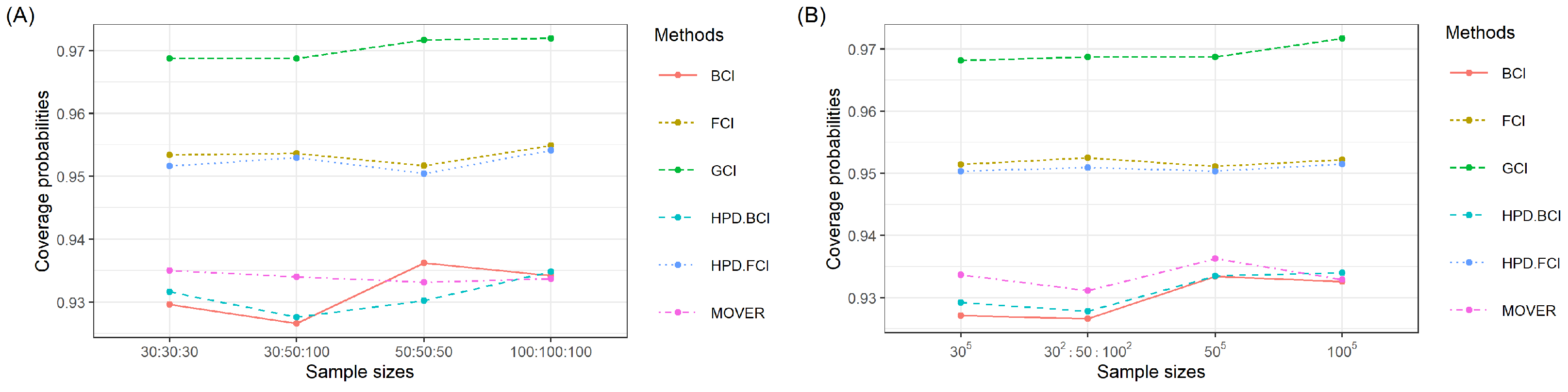
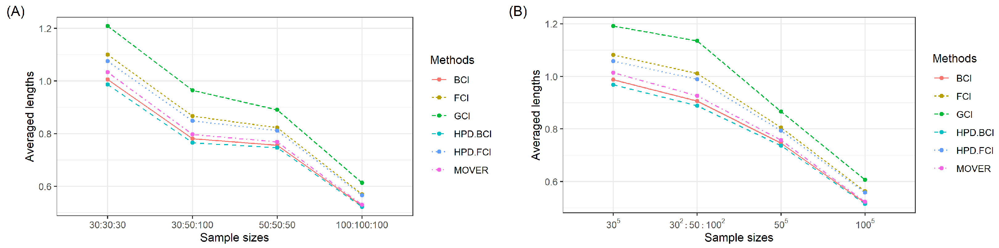
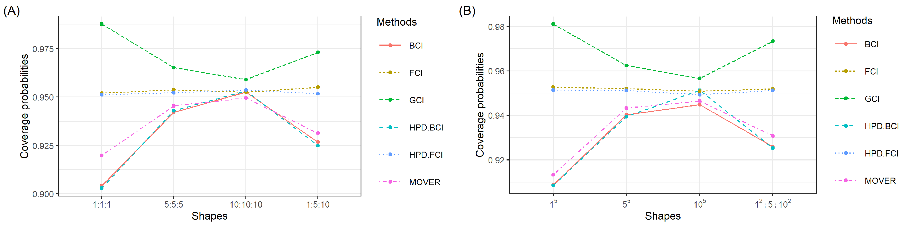
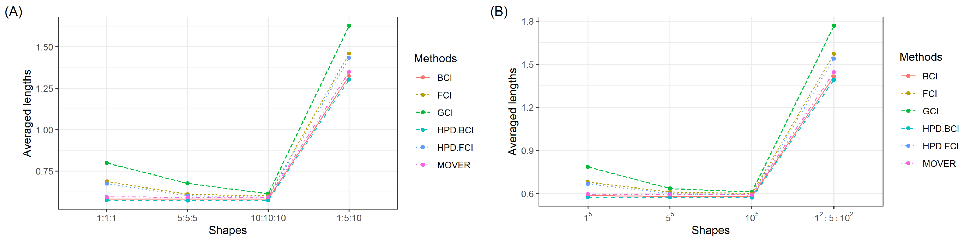
2.5. The Simulation Study

We compared the efficacies of the SCI construction approaches via a Monte Carlo simulation study based on 5000 runs. The comparison was made in terms of the coverage probability (CP) and average length (AL). The best-performing method attains a CP equal to or greater than the nominal confidence level of 0.95 together with the shortest AL. In the study, 2500 GPQs were generated for the GCI method and 20,000 iterations with a burn-in of 1000 were utilized for Gibbs sampling in conjunction with the MCMC algorithm for the Bayesian and HPD approaches. In addition, the sample sizes utilized were $n=30,50,$ or $100;$ the number of populations $\left(p\right)$ was 3 or $5;$${\mu }_i=0.5,1;$ and ${\lambda }_i=1,5,10.$

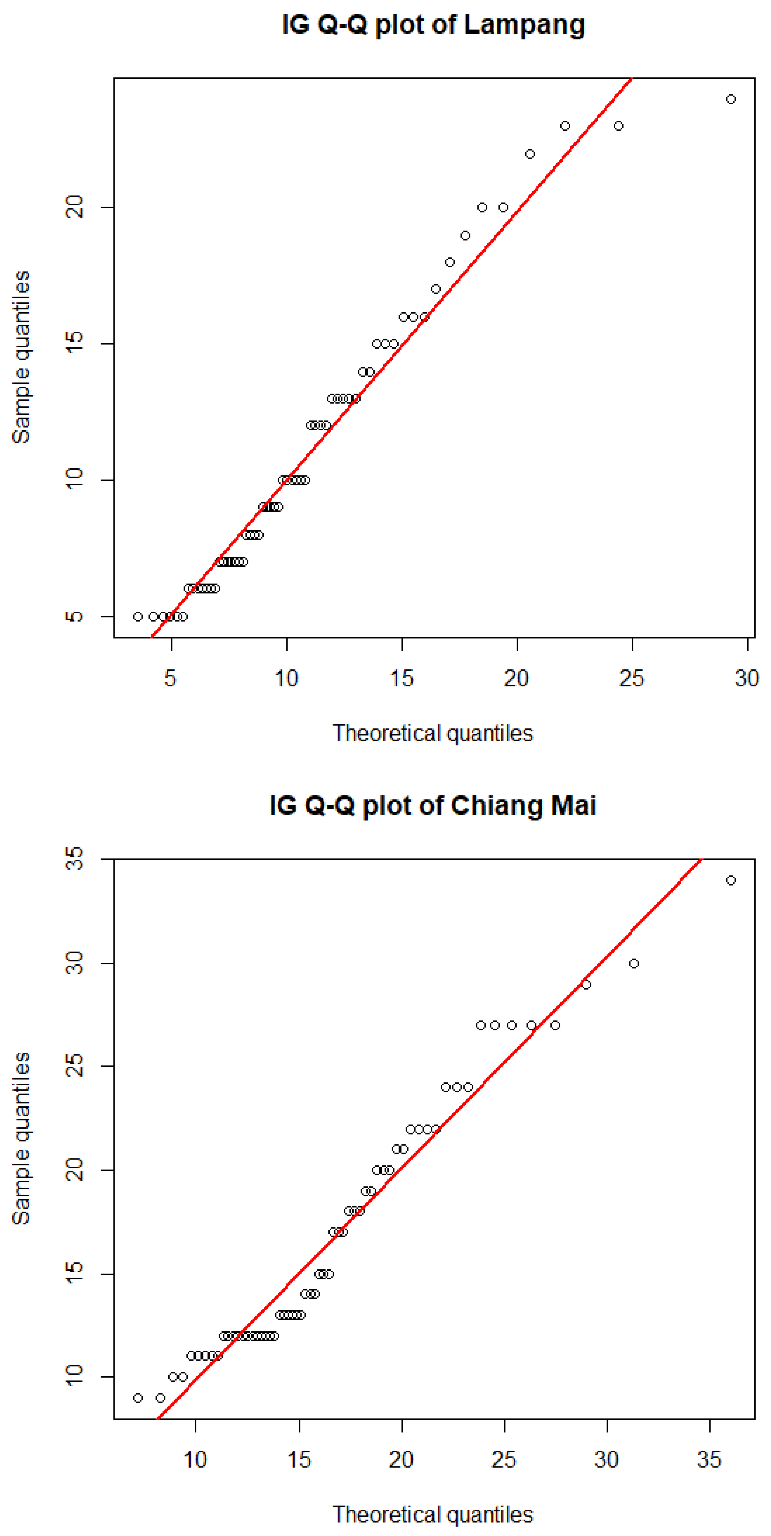
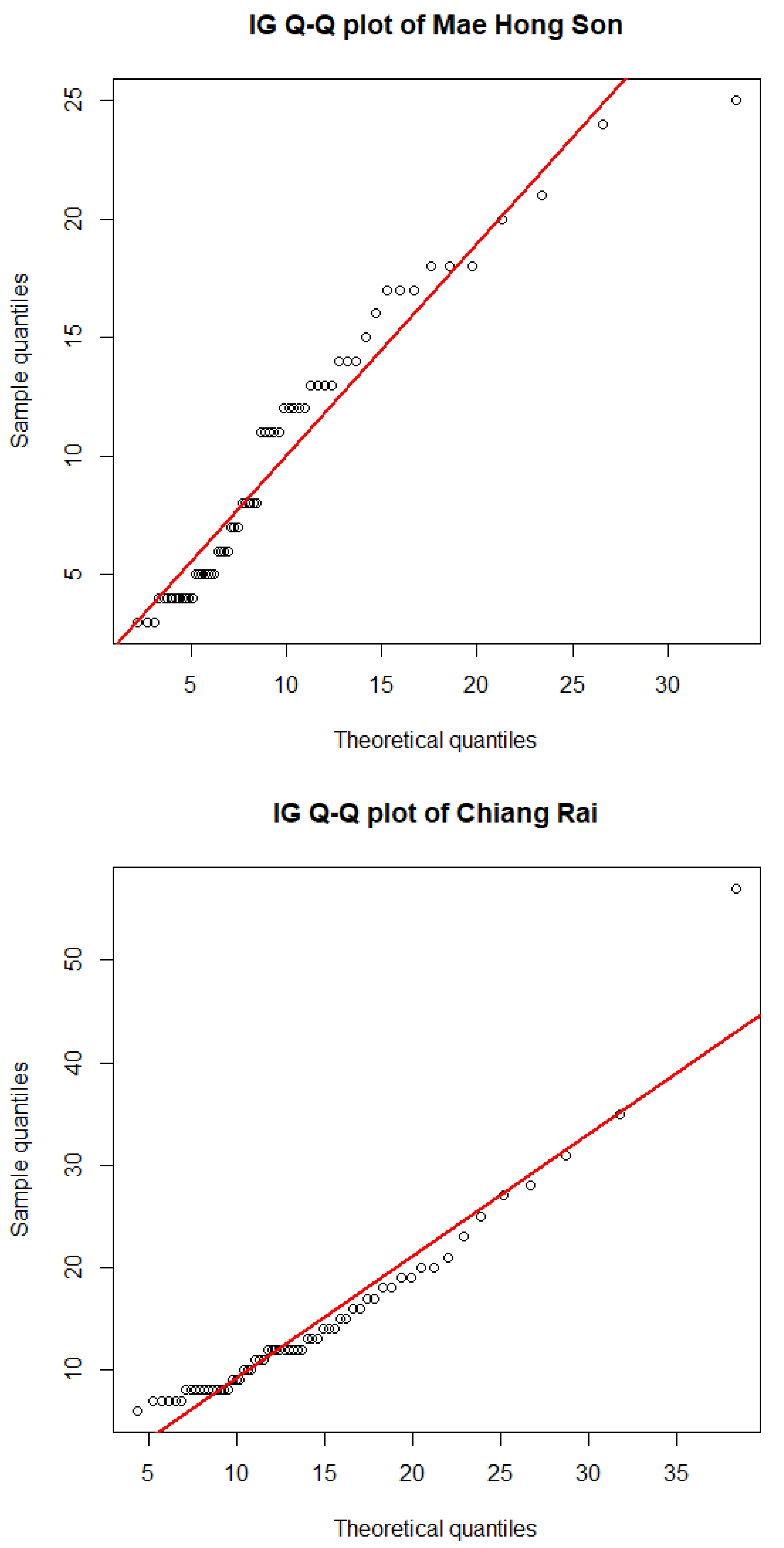
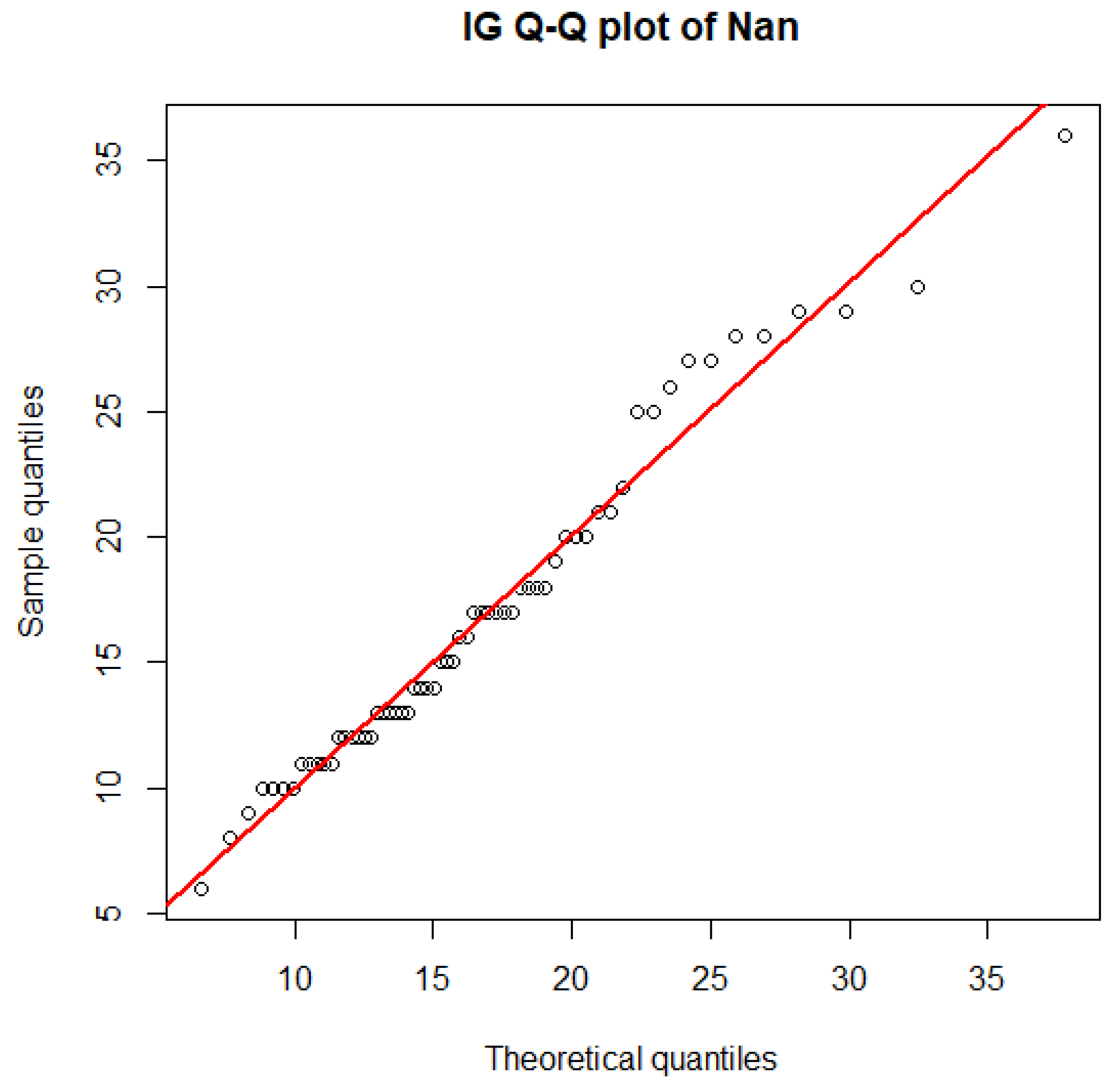
2.6. Empirical Application of the Approaches to $P{M}_{2.5}$ Datasets from Northern Thailand

Datasets of the average daily $P{M}_{2.5}$ concentrations from May to June 2022 in Lampang (N1), Chiang Mai (N2), Mae Hong Son (N3), Chiang Rai (N4), and Nan (N5) in northern Thailand were utilized to assess the effectiveness of the proposed methods in constructing the SCI for the ratios of the CVs of multiple IG distributions, the details for which can be found in Table 1 [31]. As the $P{M}_{2.5}$ datasets contain positive values, they could be modeled using a lognormal, Cauchy, exponential, Weibull, or IG distribution. Hence, the minimum Akaike information criterion (AIC) and Bayesian information criterion (BIC) were used to identify the best-fitting distribution for these data. The summary statistics for the $P{M}_{2.5}$ concentration datasets from the five provinces in northern Thailand are reported in Table 2.

Table 1. The daily $\mathit{P}{\mathit{M}}_{\mathbf{2.5}}$ data for May–June 2022 in northern Thailand by province.

Province	Daily ${\mathit{PM}}_{2.5}$
N1	15	15	14	22	24	23	13	8	9	10	9	9
	12	13	15	14	7	8	9	7	5	13	16	12
	13	20	19	23	18	20	16	12	17	16	7	6
	6	7	8	10	13	10	10	12	10	10	7	6
	5	6	5	6	5	7	5	7	9	8	6	6	5
N2	27	24	20	27	34	30	13	11	12	13	9	12
	20	18	19	22	15	12	13	12	10	19	22	15
	20	27	24	29	27	27	21	17	22	22	14	12
	12	11	10	13	17	17	15	18	24	21	18	13
	12	14	12	11	12	13	12	14	11	12	9	11	12
N3	17	24	14	25	21	18	13	8	7	6	5	8
	14	11	16	13	8	6	6	7	4	12	14	8
	12	18	17	20	18	17	15	13	13	11	5	4
	4	4	6	11	12	11	8	11	12	12	7	5
	4	4	5	3	4	4	5	5	4	5	3	3	4
N4	27	16	18	35	57	31	20	12	12	8	8	9
	12	17	17	19	13	12	13	14	7	9	20	11
	13	18	21	23	28	25	12	12	14	16	12	7
	8	8	8	9	14	15	12	15	19	12	10	7
	8	10	8	8	8	11	7	7	11	10	8	8	6
N5	25	17	22	29	36	30	20	10	12	15	11	10
	13	15	17	13	10	17	19	16	9	14	21	17
	20	25	28	29	26	28	17	20	27	27	15	12
	12	14	14	17	18	18	18	18	21	16	11	8
	10	11	12	11	13	13	12	13	13	14	12	11	6

Table 2. Parameter estimates for the five $P{M}_{2.5}$ datasets.

Province	${\mathit{n}}_{\mathit{i}}$	Min	Max	Mean	Variance	CV
N1	61	5	24	11.1148	27.5387	0.4721
N2	61	9	24	16.9672	35.2568	0.3500
N3	61	3	25	9.9016	39.8565	0.6376
N4	61	6	57	14.1803	48.1425	0.4893
N5	61	6	36	16.8525	40.9929	0.3799

3. Results

3.1. The Simulation Study

The results for $p=3$ and $p=5$ are provided in Table 3 and Table 4, respectively. The CPs for the GCI, FCI, and FCI.HPD methods were above or close to the nominal confidence level of 0.95 under all circumstances, whereas those for MOVER were slightly below it in almost all of them. In most cases, the ALs for FCI and HPD.FCI were shorter than those of the other methods, except when the shape parameter was 5 or 10, for which HPD.BCI provided the shortest ALs. Based on this evidence, we recommend using HPD.FCI and HPD.BCI to construct the SCI for the ratios between the CVs of several IG distributions. Figure 1 displays the CPs of various methods across different sample sizes. It can be observed that the GCI, FCI, and HPD.FCI methods exhibited CPs either above or close to the nominal confidence level. In contrast, the BCI, HPD.BCI, and MOVER methods provided CPs below the nominal confidence level. Figure 2 illustrates the ALs for the various methods across different sample sizes, showing a decrease in the ALs for all methods as the sample size was increased. Consequently, the HPD.FCI method outperformed the others for various parameter shapes displayed in Figure 3 and Figure 4.

Table 3. CPs and ALs for the 95% SCI for the ratios of the CVs of multiple IG distributions in the case of $p=3$.

${\mathit{n}}_1,{\mathit{n}}_2,{\mathit{n}}_3$	${\mathit{\mu }}_1,{\mathit{\mu }}_2,{\mathit{\mu }}_3$	${\mathit{\lambda }}_1,{\mathit{\lambda }}_2,{\mathit{\lambda }}_3$	CPs (ALs)
			$\mathit{G}$	$\mathit{B}$	$\mathit{H}\mathit{P}\mathit{D}.\mathit{B}\mathit{C}\mathit{I}$	$\mathit{F}$	$\mathit{H}\mathit{P}\mathit{D}.\mathit{F}\mathit{C}\mathit{I}$	$\mathit{MOVER}$
30:30:30	0.5:0.5:0.5	1:1:1	0.9812	0.9180	0.9164	0.9521	0.9500	0.9256
			(0.9665)	(0.7615)	(0.7469)	(0.8611)	(0.8410)	(0.7825)
		5:5:5	0.9617	0.9437	0.9504	0.9536	0.9528	0.9498
			(0.8168)	(0.7626)	(0.7481)	(0.7944)	(0.7782)	(0.7835)
		10:10:10	0.9517	0.9517	0.9550	0.9503	0.9500	0.9497
			(0.7976)	(0.7639)	(0.7493)	(0.7869)	(0.7712)	(0.7849)
		1:5:10	0.9603	0.9277	0.9307	0.9506	0.9501	0.9337
			(2.0073)	(1.7257)	(1.6930)	(1.8516)	(1.8118)	(1.7736)
	1:1:1	1:1:1	0.9927	0.8970	0.8953	0.9517	0.9507	0.9083
			(1.1531)	(0.7662)	(0.7515)	(0.9454)	(0.9198)	(0.7875)
		5:5:5	0.9663	0.9320	0.9363	0.9507	0.9505	0.9387
			(0.8599)	(0.7652)	(0.7507)	(0.8151)	(0.7979)	(0.7864)
		10:10:10	0.9640	0.9517	0.9526	0.9540	0.9563	0.9510
			(0.8164)	(0.7609)	(0.7463)	(0.7931)	(0.7768)	(0.7818)
		1:5:10	0.9717	0.9150	0.9163	0.9641	0.9521	0.9233
			(2.2465)	(1.7354)	(1.7023)	(1.9523)	(1.9064)	(1.7834)
30:50:100	0.5:0.5:0.5	1:1:1	0.9793	0.9157	0.9127	0.9503	0.9501	0.9207
			(0.7478)	(0.5844)	(0.5733)	(0.6630)	(0.6493)	(0.5963)
		5:5:5	0.9580	0.9333	0.9283	0.9501	0.9504	0.9400
			(0.6292)	(0.5851)	(0.5739)	(0.6119)	(0.5997)	(0.5969)
		10:10:10	0.9633	0.9530	0.9527	0.9567	0.9593	0.9563
			(0.6189)	(0.5891)	(0.5779)	(0.6093)	(0.5974)	(0.6010)
		1:5:10	0.9760	0.9383	0.9370	0.9590	0.9570	0.9430
			(1.6471)	(1.3658)	(1.3384)	(1.4984)	(1.4665)	(1.3948)
	1:1:1	1:1:1	0.9923	0.8850	0.8840	0.9521	0.9501	0.8903
			(0.8933)	(0.5887)	(0.5775)	(0.7285)	(0.7120)	(0.6007)
		5:5:5	0.9667	0.9393	0.9360	0.9523	0.9512	0.9423
			(0.6637)	(0.5886)	(0.5774)	(0.6294)	(0.6169)	(0.6007)
		10:10:10	0.9633	0.9437	0.9502	0.9523	0.9550	0.9483
			(0.6359)	(0.5913)	(0.5799)	(0.6186)	(0.6064)	(0.6032)
		1:5:10	0.9860	0.9267	0.9200	0.9560	0.9500	0.9307
			(1.8813)	(1.3540)	(1.3270)	(1.5738)	(1.5386)	(1.3830)
50:50:50	0.5:0.5:0.5	1:1:1	0.9834	0.9209	0.9181	0.9515	0.9507	0.9246
			(0.7187)	(0.5751)	(0.5681)	(0.6472)	(0.6376)	(0.5842)
		5:5:5	0.9605	0.9512	0.9503	0.9507	0.9500	0.9466
			(0.6104)	(0.5748)	(0.5677)	(0.5947)	(0.5870)	(0.5839)
		10:10:10	0.9550	0.9563	0.9548	0.9537	0.9510	0.9517
			(0.5939)	(0.5731)	(0.5660)	(0.5862)	(0.5786)	(0.5822)
		1:5:10	0.9677	0.9313	0.9257	0.9503	0.9504	0.9363
			(1.4696)	(1.2920)	(1.2762)	(1.3776)	(1.3589)	(1.3126)
	1:1:1	1:1:1	0.9930	0.8843	0.8843	0.9500	0.9500	0.8893
			(0.8478)	(0.5812)	(0.5741)	(0.7146)	(0.7024)	(0.5904)
		5:5:5	0.9723	0.9347	0.9370	0.9533	0.9500	0.9393
			(0.6375)	(0.5740)	(0.5669)	(0.6072)	(0.5991)	(0.5831)
		10:10:10	0.9607	0.9546	0.9533	0.9507	0.9507	0.9457
			(0.6163)	(0.5807)	(0.5737)	(0.6006)	(0.5928)	(0.5899)
		1:5:10	0.9807	0.9273	0.9177	0.9530	0.9507	0.9310
			(1.6256)	(1.2964)	(1.2807)	(1.4504)	(1.4289)	(1.3171)
100:100:100	0.5:0.5:0.5	1:1:1	0.9873	0.9157	0.9187	0.9520	0.9509	0.9173
			(0.4938)	(0.3993)	(0.3964)	(0.4478)	(0.4441)	(0.4024)
		5:5:5	0.9630	0.9523	0.9550	0.9563	0.9540	0.9533
			(0.4209)	(0.3982)	(0.3953)	(0.4099)	(0.4068)	(0.4012)
		10:10:10	0.9553	0.9558	0.9546	0.9513	0.9563	0.9480
			(0.4094)	(0.3972)	(0.3943)	(0.4041)	(0.4012)	(0.3964)
		1:5:10	0.9643	0.9293	0.9337	0.9516	0.9510	0.9307
			(1.0200)	(0.9058)	(0.8992)	(0.9621)	(0.9546)	(0.9127)
	1:1:1	1:1:1	0.9933	0.8963	0.8943	0.9577	0.9570	0.8983
			(0.5726)	(0.3986)	(0.3957)	(0.4891)	(0.4843)	(0.4017)
		5:5:5	0.9743	0.9513	0.9510	0.9637	0.9597	0.9537
			(0.4402)	(0.3988)	(0.3960)	(0.4200)	(0.4168)	(0.4019)
		10:10:10	0.9597	0.9541	0.9523	0.9507	0.9510	0.9467
			(0.4198)	(0.3979)	(0.3951)	(0.4097)	(0.4067)	(0.4010)
		1:5:10	0.9783	0.9187	0.9190	0.9561	0.9531	0.9213
			(1.1231)	(0.9086)	(0.9022)	(1.0144)	(1.0057)	(0.9156)

CPs greater than the nominal confidence level of 0.95 and the shortest ALs are in bold.

Table 4. CPs and ALs for the 95% SCI for ratios of the CVs of multiple IG distributions in the case of $p=5$.

${\mathit{n}}_{\mathit{i}}^5$	${\mathit{\mu }}_{\mathit{i}}^5$	${\mathit{\lambda }}_{\mathit{i}}^5$	CPs (ALs)
			$\mathit{GCI}$	$\mathit{BCI}$	$\mathit{HPD}.\mathit{BCI}$	$\mathit{FCI}$	$\mathit{HPD}.\mathit{FCI}$	$\mathit{MOVER}$
${30}^5$	$0.5^5$	$1^5$	0.9770	0.9155	0.9163	0.9502	0.9502	0.9230
			(0.9724)	(0.7639)	(0.7494)	(0.8636)	(0.8435)	(0.7850)
		$5^5$	0.9526	0.9365	0.9351	0.9515	0.9505	0.9447
			(0.8160)	(0.7615)	(0.7470)	(0.7935)	(0.7773)	(0.7825)
		${10}^5$	0.9535	0.9425	0.9502	0.9502	0.9482	0.9426
			(0.7969)	(0.7610)	(0.7466)	(0.7842)	(0.7685)	(0.7822)
		$1^2:5:{10}^2$	0.9673	0.9317	0.9329	0.9511	0.9505	0.9400
			(1.9387)	(1.6644)	(1.6327)	(1.7892)	(1.7508)	(1.7103)
	$1^5$	$1^5$	0.9915	0.8907	0.8916	0.9529	0.9511	0.8992
			(1.1591)	(0.7674)	(0.7528)	(0.9468)	(0.9212)	(0.7886)
		$5^5$	0.9685	0.9393	0.9387	0.9550	0.9525	0.9446
			(0.8531)	(0.7594)	(0.7449)	(0.8087)	(0.7917)	(0.7804)
		${10}^5$	0.9564	0.9410	0.9509	0.9503	0.9489	0.9474
			(0.8103)	(0.7552)	(0.7408)	(0.7871)	(0.7711)	(0.7761)
		$1^2:5:{10}^2$	0.9781	0.9197	0.9182	0.9501	0.9506	0.9281
			(2.1896)	(1.6669)	(1.6349)	(1.8817)	(1.8373)	(1.7124)
${30}^2:50:{100}^2$	$0.5^5$	$1^5$	0.9786	0.9224	0.9192	0.9528	0.9520	0.9268
			(0.7519)	(0.5899)	(0.5783)	(0.6693)	(0.6553)	(0.6015)
		$5^5$	0.9584	0.9396	0.9348	0.9514	0.9509	0.9444
			(0.6314)	(0.5868)	(0.5756)	(0.6130)	(0.6010)	(0.5988)
		${10}^5$	0.9544	0.9460	0.9512	0.9524	0.9515	0.9492
			(0.6170)	(0.5884)	(0.5733)	(0.6085)	(0.5965)	(0.6006)
		$1^2:5:{10}^2$	0.9669	0.9242	0.9266	0.9530	0.9521	0.9290
			(2.2674)	(1.8606)	(1.8224)	(2.0485)	(2.0032)	(1.9028)
	$1^5$	$1^5$	0.9936	0.8938	0.8956	0.9574	0.9558	0.8992
			(0.8959)	(0.5923)	(0.5811)	(0.7335)	(0.7169)	(0.6047)
		$5^5$	0.9638	0.9302	0.9262	0.9502	0.9500	0.9354
			(0.6613)	(0.5879)	(0.5768)	(0.6280)	(0.6156)	(0.5999)
		${10}^5$	0.9546	0.9358	0.9541	0.9500	0.9430	0.9388
			(0.6314)	(0.5867)	(0.5755)	(0.6133)	(0.6012)	(0.5988)
		$1^2:5:{10}^2$	0.9789	0.9207	0.9149	0.9530	0.9522	0.9256
			(2.6288)	(1.8612)	(1.8226)	(2.1788)	(2.1275)	(1.9034)
${50}^5$	$0.5^5$	$1^5$	0.9825	0.9201	0.9188	0.9526	0.9502	0.9239
			(0.7187)	(0.5747)	(0.5677)	(0.6467)	(0.6372)	(0.5839)
		$5^5$	0.9592	0.9420	0.9399	0.9504	0.9503	0.9465
			(0.6102)	(0.5745)	(0.5675)	(0.5944)	(0.5867)	(0.5837)
		${10}^5$	0.9512	0.9486	0.9502	0.9435	0.9448	0.9421
			(0.5962)	(0.5752)	(0.5682)	(0.5882)	(0.5808)	(0.5843)
		$1^2:5:{10}^2$	0.9686	0.9322	0.9319	0.9510	0.9502	0.9365
			(1.4379)	(1.2574)	(1.2420)	(1.3447)	(1.3264)	(1.2775)
	$1^5$	$1^5$	0.9825	0.9201	0.9188	0.9526	0.9502	0.9239
			(0.7187)	(0.5747)	(0.5677)	(0.6467)	(0.6372)	(0.5839)
		$5^5$	0.9683	0.9377	0.9390	0.9533	0.9527	0.9427
			(0.6407)	(0.5764)	(0.5693)	(0.6098)	(0.6017)	(0.5855)
		${10}^5$	0.9624	0.9473	0.9510	0.9535	0.9526	0.9505
			(0.6081)	(0.5727)	(0.5657)	(0.5927)	(0.5850)	(0.5819)
		$1^2:5:{10}^2$	0.9762	0.9194	0.9183	0.9522	0.9512	0.9241
			(1.6001)	(1.2607)	(1.2453)	(1.4181)	(1.3969)	(1.2807)
${100}^5$	$0.5^5$	$1^5$	0.9808	0.9136	0.9144	0.9504	0.9502	0.9154
			(0.4936)	(0.3991)	(0.3962)	(0.4479)	(0.4441)	(0.4021)
		$5^5$	0.9601	0.9441	0.9508	0.9503	0.9484	0.9454
			(0.4209)	(0.3989)	(0.3960)	(0.4107)	(0.4076)	(0.4025)
		${10}^5$	0.9587	0.9518	0.9514	0.9548	0.9543	0.9536
			(0.4112)	(0.3986)	(0.3958)	(0.4056)	(0.4025)	(0.4017)
		$1^2:5:{10}^2$	0.9707	0.9358	0.9353	0.9516	0.9501	0.9379
			(0.9934)	(0.8765)	(0.8702)	(0.9339)	(0.9264)	(0.8831)
	$1^5$	$1^5$	0.9926	0.8935	0.8936	0.9515	0.9514	0.8953
			(0.5746)	(0.3996)	(0.3966)	(0.4905)	(0.4857)	(0.4026)
		$5^5$	0.9691	0.9518	0.9508	0.9535	0.9545	0.9427
			(0.4412)	(0.3997)	(0.3968)	(0.4210)	(0.4177)	(0.4027)
		${10}^5$	0.9618	0.9461	0.9514	0.9524	0.9508	0.9479
			(0.4208)	(0.3987)	(0.3958)	(0.4103)	(0.4073)	(0.4017)
		$1^2:5:{10}^2$	0.9796	0.9238	0.9244	0.9529	0.9526	0.9250
			(1.0932)	(0.8754)	(0.8690)	(0.9819)	(0.9735)	(0.8821)

CPs greater than the nominal confidence level of 0.95 and the shortest ALs are in bold.

Figure 1. CPs for the 95 % SCI derived using the various methods for various sample sizes in the cases of (A) $p=3$ and (B) $p=5$.

Figure 2. ALs for the 95% SCI derived using the various methods for various sample sizes in the cases of (A) $p=3$ and (B) $p=5$.

Figure 3. CPs for the 95% SCI derived using the various methods for various parameter shapes in the cases of (A) $p=3$ and (B) $p=5$.

Figure 4. ALs for the 95% SCI using the various methods for various parameter shapes in the cases of (A) $p=3$ and (B) $p=5$.

3.2. Empirical Application of the Methods to $P{M}_{2.5}$ Datasets from Northern Thailand

The AIC and BIC results in Table 5 and Table 6, respectively, indicate that the positive values observed in the $P{M}_{2.5}$ datasets from the five provinces adhere to the characteristics of an IG distribution. The AIC and BIC values of the inverse Gaussian distribution and the lognormal distribution were not significantly different because both distributions are based on the right-skewed characteristic. In this situation, the model for the inverse Gaussian distribution was considered to be the best due to it providing the lowest AIC and BIC values. Furthermore, the quantile–quantile (Q-Q) plots for the IG distribution confirm this finding in Figure 5.

Table 5. The AIC values for evaluating the distribution for the daily $P{M}_{2.5}$ data.

Province	Distribution
	Inverse Gaussian	Lognormal	Cauchy	Exponential	Weibull
N1	360.5187	361.6107	398.1535	417.8094	369.3542
N2	383.4496	384.1563	419.3525	469.4165	395.0606
N3	370.8679	372.6417	416.3720	403.7094	375.7245
N4	391.3827	391.526	415.1157	447.5264	415.2512
N5	391.1549	391.3873	418.4176	468.5866	400.4491

Table 6. The BIC values for evaluating the distribution for the daily $P{M}_{2.5}$ data.

Province	Distribution
	Inverse Gaussian	Lognormal	Cauchy	Exponential	Weibull
N1	364.7405	365.8324	402.3752	419.9202	373.576
N2	387.6714	388.3781	423.5742	471.5274	399.2824
N3	375.0896	376.8635	420.5937	405.8203	379.9462
N4	395.6044	395.7477	419.3375	449.6373	419.473
N5	395.3767	395.6091	422.6394	470.6995	404.6708

Figure 5. Q-Q plots for fitting the distribution for the $P{M}_{2.5}$ datasets.

The 95% SCIs for the daily $P{M}_{2.5}$ datasets from five provinces in northern Thailand are reported in Table 7. The results show that the AL for HPD.BCI was the shortest, which corresponds well with the simulation results. Therefore, it is a good choice for constructing the SCI for the ratios of the CVs of the five $P{M}_{2.5}$ datasets.

Table 7. The ratios of the CV of the daily $P{M}_{2.5}$ datasets with the nominal 95% SCI.

Provinces	GCI			Bayesian			HPD.Bayesian			FCI			HPD.FCI			MOVER
	Lower	Upper	Length	Lower	Upper	Length	Lower	Upper	Length	Lower	Upper	Length	Lower	Upper	Length	Lower	Upper	Length
N1/N2	1.0344	1.7718	0.7374	1.0477	1.7314	0.6837	1.0339	1.7101	0.6762	1.0389	1.7479	0.7090	1.0235	1.7284	0.7049	1.0439	1.7437	0.6998
N1/N3	0.5431	0.9937	0.4506	0.5741	0.9534	0.3793	0.5629	0.9387	0.3758	0.5617	0.9681	0.4064	0.5548	0.9575	0.4027	0.5730	0.9570	0.3840
N1/N4	0.7192	1.2710	0.5518	0.7472	1.2426	0.4954	0.7285	1.2181	0.4896	0.7346	1.2608	0.5262	0.7189	1.2410	0.5221	0.7466	1.2471	0.5005
N1/N5	0.9337	1.6365	0.7028	0.9647	1.5999	0.6352	0.9400	1.5693	0.6293	0.9564	1.6256	0.6692	0.9273	1.5863	0.6590	0.9616	1.6061	0.6445
N2/N3	0.4138	0.7229	0.3091	0.4261	0.7083	0.2822	0.4214	0.6996	0.2782	0.4206	0.7202	0.2996	0.4107	0.7062	0.2955	0.4247	0.7094	0.2847
N2/N4	0.5314	0.9443	0.4129	0.5538	0.9202	0.3664	0.5438	0.9054	0.3616	0.5486	0.9317	0.3831	0.5359	0.9127	0.3768	0.5534	0.9244	0.3710
N2/N5	0.7081	1.1962	0.4881	0.7154	1.189	0.4736	0.6987	1.1677	0.4690	0.7106	1.1997	0.4891	0.6972	1.1804	0.4832	0.7127	1.1905	0.4778
N3/N4	0.9636	1.7625	0.7989	1.0110	1.6862	0.6752	0.9839	1.6482	0.6643	0.9905	1.7175	0.7270	0.9722	1.6856	0.7134	1.0082	1.6841	0.6759
N3/N5	1.2584	2.2576	0.9992	1.3064	2.1611	0.8547	1.2777	2.1263	0.8486	1.2804	2.2012	0.9208	1.2420	2.1498	0.9078	1.2985	2.1689	0.8704
N4/N5	0.9729	1.7170	0.7441	0.9977	1.6628	0.6651	0.9750	1.6289	0.6539	0.9884	1.6866	0.6982	0.9539	1.6419	0.6880	0.9965	1.6645	0.6680

The 95% SCIs for the daily $P{M}_{2.5}$ dataset from five provinces in northern Thailand in May–June 2022 are reported in Table 7. The results show the AL of the HPD.BCI was the shortest, which corresponds with the simulation results. Therefore, it is a good choice for constructing the SCI for the ratios of the CVs of the $P{M}_{2.5}$ datasets from the five provinces in northern Thailand.

4. Discussion

Wasana et al. [32] utilized the FCI and HPD.FCI methods to construct CIs for the ratio of the CVs of two IG distributions. Examination of the efficacies of these methods revealed that HPD.FCI is the most suitable in this scenario. Building on this idea, we developed estimates for the SCI for the ratios of the CVs of multiple IG populations. The results reveal that the CPs and ALs for the 95% SCI for $p=3$ were similar to those for $p=5$ across various sample sizes. Notably, for a shape parameter of 10, the HPD.BCI approach performed the best. In contrast, for shape parameter values of 1 or 5, the HPD.FCI approach was the most suitable for all of the situations studied. In addition, the ALs of the approaches decreased with an increasing sample size. The methods were applied in an empirical investigation of the ratios of CVs of $P{M}_{2.5}$ datasets following IG distributions for five provinces in northern Thailand. The findings aligned with the results of the simulation study, indicating that the HPD.BCI and HPD.FCI methods are the most suitable depending on the scenario. By utilizing our approach for the SCI of the CVs of several $P{M}_{2.5}$ datasets following IG distributions in a decision-making process, policymakers can enhance the effectiveness and adaptability of measures aimed at mitigating $P{M}_{2.5}$ pollution, ultimately safeguarding public health and the environment. The proposed approaches could be used in the spatial analysis of $P{M}_{2.5}$ concentrations to identify areas with high pollution levels. Policymakers can use the information to develop new air pollution prevention and control action plans in key areas.

5. Conclusions

In this research, six approaches (GCI, BCI, HPD.BCI, FCI, HPD.FCI, and MOVER) to constructing the SCI for the ratios of CVs of multiple IG distributions were investigated. The outcomes from a simulation study and an empirical study involving $P{M}_{2.5}$ datasets in terms of the CP and AL suggest that the HPD.FCI method was the most appropriate in most instances. However, it is noteworthy that HPD.BCI demonstrated effectiveness in certain scenarios involving three or five IG populations. Although the proposed HBD.BCI and HBD.FCI methods have many advantages, they have two limitations. First, the choice of prior distribution in the Bayesian analysis can significantly impact the results. Specifying informative priors may be challenging for areas where prior knowledge is limited or where the environmental conditions are diverse. Second, Bayesian and fiducial methods frequently entail computationally intensive tasks, and the efficiency of these methods can be influenced by factors such as the scale of the data or the complexity of the model, particularly for diverse real-world scenarios. These limitations will be addressed in future studies. Adaptive Bayesian and fiducial methods, which can be adjusted to different environmental conditions by incorporating contextual information, will be developed. Moreover, parallel processing or distributed computing could be carried out to more efficiently handle the computational complexity, along with exploring advancements in Bayesian computation, such as MCMC algorithms, to enhance the speed and scalability of the analysis. The investigation also reveals the limitations of using different priors. Future investigations will also be conducted to refine the choice of prior and to construct the SCI for the ratios of the percentiles of several IG distributions.