Inverse Problem for the Moisture Transfer Equation: Development of a Method for Finding the Unknown Parameter and Proof of the Convergence of the Iterative Process

Abstract

This study develops a mathematical model for soil moisture diffusion, addressing the inverse problem of determining both the diffusion coefficient and the variation coefficient in a nonlinear moisture transfer equation. The model incorporates specific boundary and initial conditions and utilizes experimentally measured moisture values at a boundary point as input data. An iterative method, based on an explicit gradient scheme, is introduced to estimate the soil parameters. The initial boundary value problem is discretized, leading to a difference analog and the formulation of a conjugate difference problem. Iterative formulas for calculating the unknown parameters are derived, with a priori estimates ensuring the convergence of the iterative process. Additionally, the research establishes the convergence of the numerical model itself, providing a rigorous foundation for the proposed approach. The study also emphasizes symmetry in moisture calculations, ensuring consistency regardless of the calculation direction (from right to left or left to right) and confirming that moisture distribution remains symmetric within specified intervals. This preservation of symmetry enhances the model’s robustness and accuracy in parameter estimation. The numerical simulations were successfully conducted over a 7-day period, demonstrating the model’s reliability. The discrepancy between the numerical predictions and experimental observations remained within the margin of measurement error, confirming the model’s accuracy.

1. Introduction

Moisture measurement plays a critical role in various fields, including agriculture, environmental science, civil engineering, and material science. Accurate modeling and prediction of moisture transfer are essential for optimizing irrigation systems [1], preventing soil erosion [2], improving building insulation [3], and ensuring the durability of materials [4]. Despite significant progress in recent years, existing models often face limitations when dealing with non-linear dynamics and complex boundary conditions, especially in media with contact boundaries. In agriculture, understanding moisture dynamics is essential for efficient water management, improving crop yields, and reducing water waste [5]. Recent studies have shown that improved moisture transfer models can significantly enhance irrigation practices by predicting soil moisture behavior more accurately [6]. In civil engineering, moisture-related problems such as mold growth, material degradation, and foundation damage pose serious challenges [7]. Advanced moisture models can help predict these issues and mitigate their impacts through better design and maintenance practices. Moreover, in material science, the ability to predict moisture behavior in porous materials is crucial for improving product durability, especially in humid environments [8]. These applications highlight the wide-reaching impact of accurate moisture transfer models across different scientific disciplines.

Basic Approaches to Mathematical Modeling of Moisture Transfer

Mathematical models of most natural processes are based on the concept of continuum [9,10]. Analyzing known models, the authors of [11] consider it possible to accept the following assumptions: moisture transfer in the soil develops under the influence of capillary and gravitational forces.

Taking this into account, the equation of fluid motion when the soil is saturated can be described using Darcy’s law [12]. In this case, the speed of fluid movement is proportional to the pressure gradient:

$$\begin{array}{c}\hfill {\displaystyle \frac{\partial W}{\partial t}}=\mathrm{div}\left(D\left(W\right)\nabla H\right),\end{array}$$

(1)

where $D\left(W\right)$ is the coefficient of moisture conductivity, which, according to [12], follows the dependence $D\left(W\right)=E{e}^{aW}$. This coefficient also depends on the coordinates x, y, z, and W—volumetric soil moisture, H—pressure, and t—time.

Soil moisture can vary depending on movement. If, at the initial period, the soil has an uneven moisture distribution in depth, over time, the moisture content will increase in drier layers according to the diffusion law. The direction of the soil moisture gradient will correspond to the layers where it is lower. If moisture moves from the larger to the smaller, then the process of moisture transfer is described by Equation (1). However, in some cases, moisture moves from less to more, a phenomenon known as the Allaire effect, described using the concept of fractured porous soil. A correction term is introduced into the moisture transfer equation to account for this effect, leading to the Allaire model [13]:

$$\begin{array}{c}\hfill {\displaystyle \frac{\partial W}{\partial t}}={\displaystyle \frac{\partial }{\partial x}}\left(D{\displaystyle \frac{\partial W}{\partial x}}+A{\displaystyle \frac{\partial W}{\partial x\partial t}}\right),\end{array}$$

(2)

where A and D are proportionality factors.

A porous medium is primarily described as a continuous medium, the properties of which are not expressed through the constituent elements but are described based on indicators averaged over a certain volume [14,15]. Soil is characterized by its moisture-holding capacity, i.e., the ability to retain a certain amount of moisture that does not flow into the underlying layers. The water regime of the soil depends on its properties, as well as climatic and weather conditions. The soil—the upper fertile layer of the earth’s surface, as well as the underlying soils—is a three-phase structure consisting of a solid phase, a liquid phase, and gas (air), as shown in Figure 1.

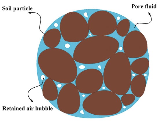
Figure 1. Soil structure with gas-air pores.

Soil moisture capacity is a quantitative value that characterizes the soil’s water-holding capacity. One of the simple models of the theory of moisture movement in soil is based on solving the water balance equation of the soil profile using the Darcy equation and the continuity equation (Richards Equation) [16]. The second fundamental physical law necessary for modeling moisture movement in soil is the law of conservation of matter [9]. The physical meaning of the Richards equation lies in describing water movement in the soil. By setting small time intervals in the vertical coordinate for elementary layers, it is possible to determine the distribution of moisture in the soil profile, taking into account the initial conditions, precipitation, irrigation, water consumption of plants, and other factors [12,17]. Soil hydraulic conductivity is understood as its conductivity under the influence of soil moisture potential gradients [13]. The coefficient of hydraulic conductivity depends on soil moisture: it increases with increasing soil moisture and reaches a maximum in moisture-saturated soil. In this case, it is referred to as the filtration coefficient, but it is applicable to soils unsaturated with water.

A number of researchers note that for soils unsaturated with water, the value of the moisture conductivity coefficient is significantly determined by soil moisture [18]. A slight reduction in moisture content can lead to a significant decrease in hydraulic conductivity, which can be explained by a decrease in volumetric conductivity. The theory of moisture movement in soil is based on the assumption of the Newtonian nature of the liquid, which does not exhibit shear resistance and has constant viscosity at a certain temperature.

The patterns of dependence of hydraulic conductivity indicators on soil moisture differ for different types of soil [12]. Currently, methods of mathematical modeling of hydraulic conductivity are becoming widespread [17,19,20,21]. It is noted that experimental methods and approaches require further improvement [22]. The developed mathematical models of moisture transfer must satisfy several requirements [11], including simplicity, the inclusion of well-studied water-physical characteristics of the soil, and the use of universal numerical solution algorithms.

It should be noted that several issues of moisture transfer were studied in works [3,23]. In [24], various computerized models for managing the water regime during irrigation were developed, although these models did not explicitly account for the production processes of plant development.

In this context, some studies have focused on improving information support for tasks related to the automation and management of soil water regimes [17]. This can be achieved through optimization algorithms, the use of calculated values and reference databases, and modern methods in monitoring the initial soil regime using automated instruments and measuring technical means of remote sensing [20]. A computer experiment typically involves using a mathematical model as the test object, with external influences, model parameters, or subprocess algorithms acting as the variable experimental conditions [11,21,24,25,26,27,28,29,30].

Scientists have been studying combined irrigation technologies [31,32,33,34]. Comprehensive descriptions of irrigation systems can be found in [35,36]. The fractal and symmetrical properties of soil colloids have been investigated in [37]. Ecological and economic regulation, taking into account transboundary environmental pollution, was studied in [38], with mathematical modeling used to describe the processes of heat and moisture transfer. Among all the studies, works devoted to the theories of inverse and ill-posed problems hold a special place. Inverse problems of various processes were studied in [38,39,40,41,42]. The efficiency of irrigation can be significantly improved through the application of information technologies and technical-economic optimization, including in the management of reclamation activities, as described in publications [43]. The development of new promising technical means is presented in the patent [44].

This study proposes a novel numerical method for solving the inverse problem of moisture transfer in soil, validated against experimental data. By determining multiple transfer coefficients simultaneously, our model provides a robust solution that can be applied to diverse real-world challenges. The model incorporates uncertainty quantification, making it reliable for practical use in fields like agriculture, environmental science, and civil engineering. The approach is highly applicable for real-time moisture monitoring and prediction.

The following sections will delve into the intricacies of the problem at hand. Section 2 describes the experimental setup and governing equations necessary for understanding the moisture dynamics within the soil. It introduces the discrete numerical model employed to simulate these processes. In Section 3 the conjugate problem is defined, and the algorithm developed to solve it is detailed. The mathematical techniques and iterative methods used in the solution process are thoroughly explained. The most crucial is Section 4 of this article; it proves the convergence of the numerical model. Rigorous mathematical analysis is presented to establish the reliability and accuracy of the iterative processes used. Section 5 illustrates the results obtained from the numerical simulations. Detailed analysis and interpretation of the data are provided, offering insights into the practical implications of the findings.

2. Inverse Problem

2.1. Experimental Setup and Mathematical Modeling of the Problem

To use one-dimensional equations of moisture conductivity, we created the container shown in Figure 2. The side edges of which are moisture-proof. Thus, it leads to symmetry boundary conditions along z axis [45]. The end sides of the container are covered with fine rectangular mesh so that soil or soil cannot leave the container. The container is filled with soil and the end faces are closed with lids. The process of moisture transfer in the container is investigated.

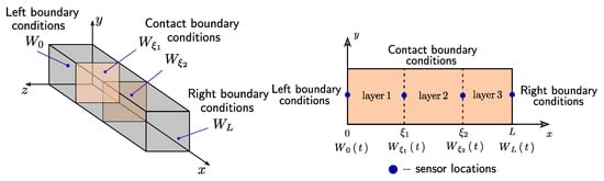
Figure 2. Experimental set-up illustration with appropriate boundary conditions position (left), scheme of the sensor locations along the container (right).

If the conditions of moisture insulation along all side faces are met, then the process of moisture transfer in the container is described by the one-dimensional moisture transfer equation

$$\begin{array}{c}\hfill {\displaystyle \frac{\partial W}{\partial t}}={\displaystyle \frac{\partial }{\partial x}}\left(D\left(W\right){\displaystyle \frac{\partial W}{\partial x}}+A{\displaystyle \frac{{\partial }^{2}W}{\partial x\partial t}}\right),\left(x,t\right)\in Q,\end{array}$$

(3)

where $Q=\left(0,x\right)\times \left(0,t_{max}\right)$, x—container length shown in Figure 2.

At the initial moment of time ($t=0$), we filled the container with soil and considered the distribution of moisture along the horizontal axis to be known. Typically this condition is written in the form

$$\begin{array}{c}\hfill W(x,0)=W_0\left(x\right),x\in (0,H)\end{array}$$

(4)

Neumann boundary conditions will be used. On the left boundary, we assume that there is no inflowing flow. This condition is equivalent to the fact that the left end of the container is closed with a heat-insulated lid. On the right boundary of the region, the inflowing flow is specified. That is, the right end is closed with a mesh cover, which allows the inflow to flow into the interior of the area. The above can be written as follows

$$\begin{array}{c}\hfill {\displaystyle \frac{\partial W\left(0,t\right)}{\partial x}}=0,{\left.\left(D\left(W\right){\displaystyle \frac{\partial W}{\partial x}}+A{\displaystyle \frac{{\partial }^{2}W}{\partial x\partial t}}\right)\right|}_{x=H}=f\left(t\right),t\in \left(0,t_{max}\right)\end{array}$$

(5)

Inverse problem. Using the mathematical model (3)–(5) we will solve the inverse problem. Using measured moisture values at the $x=H$ boundary over a long period of time $t=t_{max}$

$$\begin{array}{c}\hfill w_g\left(t\right),t\in \left(0,t_{max}\right)\end{array}$$

(6)

It is necessary to develop a method for finding moisture

$$\begin{array}{c}\hfill D\left(W\right)=E{e}^{aW},A,f\left(t\right).\end{array}$$

(7)

2.2. Discrete Problem

The segment $(0,H)$ is divided into N equal parts with step $\Delta x=H/N$, and the segment $(0,t_{max})$ is divided into m equal parts with step $\Delta t=t_{max}/m$. In the constructed mesh area

$$\begin{array}{c}\hfill \omega =\{x_i=i\ast \Delta x,t_j=j\ast \Delta t; i=0,1,\dots ,N; j=0,\dots ,m\}\end{array}$$

(8)

A discrete analog of the problem is studied (3)–(5) [46]:

$$\begin{array}{c}\hfill {\displaystyle \frac{y_i^{j+1}-y_i^j}{\Delta t}}=\left(D\left(y_{i+1}^j\right)y_{ix}^{j+1}+A\ast y_{ix,t}^{j+1}\right)\overline{x}\end{array}$$

(9)

where

$$\begin{array}{c}\hfill y_{ix}^{j+1}={\displaystyle \frac{y_{i+1}^{j+1}-y_i^{j+1}}{\Delta x}},y_{ix,\overline{t}}^{j+1}={\displaystyle \frac{y_{i,x}^{j+1}-y_{i,x}^j}{\Delta t}}\end{array}$$

(10)

$$\begin{array}{c}\hfill y_i^0=W_0\left(x\right),i=0,1,\dots ,N\end{array}$$

(11)

$$\begin{array}{c}\hfill y_1^{j+1}=y_0^{j+1},D\left(y_N^j\right)y_{N-1,x}^{j+1}+A{y}_{N-1,x,\overline{t}}^{j+1}=f\left(t_{j+1}\right)\end{array}$$

(12)

Here, $y_i^{j+1}$ is an approximate value $W\left(x,t\right)=W_i^{j+1}$. For the sake of clarity, the methodology to solve discrete problem by Thomas’ method is given in Appendix A.

After applying Thomas’ method the question arises: is the denominator of the fraction (A21) different from zero? To answer this question, we check the conditions for the computational stability of the scalar sweep method.

In our case there is

Theorem 1.

If $0<{\alpha }_1<1,B_i>A_i+C_i$, $i=1,2,\dots ,N$, then all coefficients of the sweep formula do not exceed 1, i.e.,

$$\begin{array}{c}\hfill 0<{\alpha }_i<1,i=2,3,\dots ,N.\end{array}$$

(13)

Proof. 

Direct inspection shows that

$$\begin{array}{c}\hfill 0<{\alpha }_1={\displaystyle \frac{A_1}{1+A_1}}<1\end{array}$$

(14)

On the other hand, from (A1) the equality follows

$$\begin{array}{c}\hfill B_i=A_i+C_i+1,i=1,2,\dots ,N-1\end{array}$$

(15)

therefore, $B_i>A_i+C_i,i=1,2,\dots ,N-1$. It follows that all the conditions of the theorem are met. It means that $1-{\alpha }_N>0$.   □

3. Method for Solving the Inverse Problem

3.1. Conjugate Problem

The required quantities $D\left(W\right),A,f\left(t\right)$ are sought iteratively. In this case, the solution of the system (9)–(12) will depend on the iteration number n, i.e.,

$$\begin{array}{c}\hfill Y_i^j\left(n\right),i=0,1,\dots ,N;j=0,1,\dots ,m-1.\end{array}$$

(16)

This means that the problem (9)–(12) is written in the form

$$\begin{array}{c}\hfill {\displaystyle \frac{Y_i^{j+1}\left(n\right)-Y_i^j\left(n\right)}{\Delta t}}={\displaystyle \frac{{\sigma }_i^{j+1}\left(n\right)-{\sigma }_{i-1}^j\left(n\right)}{\Delta x}}\end{array}$$

(17)

$$\begin{array}{c}\hfill \begin{array}{cc}\hfill & {\sigma }_i^{j+1}\left(n\right)=D\left(Y_{i+1}^{j+1}\left(n\right)Y_{ix}^{j+1}+A\times Y_{ix\overline{t}}^{j+1}\right)\hfill \\ \hfill & i=0,1,\dots ,N-1;j=0,1,\dots ,m-1.\hfill \end{array}\end{array}$$

(18)

$$\begin{array}{c}\hfill Y_i^0\left(n\right)=W_0\left(x_i\right),i=0,1,\dots ,N.\end{array}$$

(19)

$$\begin{array}{c}\hfill Y_1^{j+1}\left(n\right)=Y_0^{j+1}\left(n\right),{\sigma }_{N-1}^{j+1}\left(n\right)=f^{j+1}\left(n\right)\end{array}$$

(20)

Additionally, the measured moisture value is set on the right border of the area $x=H$,

$$\begin{array}{c}\hfill w_g^{j+1},j=0,1,\dots ,m-1.\end{array}$$

(21)

Using (17)–(111) for the function

$$\begin{array}{c}\hfill \Delta Y_i^{j+1}=Y_i^{j+1}\left(n+1\right)-Y_i^j\left(n\right)\end{array}$$

(22)

An auxiliary difference problem is constructed

$$\begin{array}{c}\hfill \begin{array}{c}\hfill \Delta Y_{i,\overline{t}}^{j+1}=\Delta {\sigma }_{i,x}^{j+1},\Delta {\sigma }_i^{j+1}={\sigma }_i^{j+1}\left(n+1\right)-{\sigma }_i^{j+1}\left(n\right)\\ \hfill i=0,1,\dots ,N-1; j=0,1,\dots ,m-1.\end{array}\end{array}$$

(23)

$$\begin{array}{c}\hfill \Delta Y_i^0=0,i=0,1,\dots ,N\end{array}$$

(24)

$$\begin{array}{c}\hfill Y_{0,x}^{j+1}=0\Delta {\sigma }_{N-1}^{j+1}=\Delta f^{j+1}\end{array}$$

(25)

After the multiplication of (23) by an arbitrary grid function $U_i^j$ and summing over i and j one needs to perform several mathematical steps to derive a conjugate problem (See Appendix B. Then, following the rule for choosing the boundary condition of the conjugate problem [46], we derive the conjugate problem:

$$\begin{array}{c}\hfill \begin{array}{cc}\hfill & U_{i\overline{t}}^{j+1}+{\left(D\left(Y_{i+1}^j\right)U_{i\overline{x}}^j-A\times U_{i\overline{x}\overline{t}}^{j+1}\right)}_{\overline{x}}=0,\hfill \\ \hfill & i=1,2,\dots ,N-1; j=m-1,m-2,\dots ,0,\hfill \\ \hfill & U_i^m=0,i=0,1,\dots ,N,\hfill \\ \hfill & U_{i\overline{x}}^j=0,j=m-1,m-2,\dots ,0\hfill \\ \hfill & D\left(Y_N^j\right)U_{N\overline{x}}^j-A\times U_{N\overline{x}\overline{t}}^{j+1}=2\left(Y_N^{j+1}-w_g^{j+1}\right)\hfill \\ \hfill & j=m-1,m-2,\dots ,0\hfill \end{array}\end{array}$$

(26)

The conjugate problem (26) significantly simplifies the equality (A38) and it is written in the form:

$$\begin{array}{c}\hfill 2\sum _{j=0}^{m-1}\Delta Y_N^{j+1}\left(Y_N^{j+1}-w_g^{j+1}\right)\Delta t=\sum _{j=0}^{m-1}\Delta f^{j+1}{U}_N^j\Delta t+I_2+I_4\end{array}$$

(27)

3.2. Algorithm for Solving the Conjugate Problem

Let us rewrite the difference equation of the system (26) in the form

$$\begin{array}{c}\hfill {\left(D\left(Y_{i+1}^j\right)U_{i,x}^j+{\displaystyle \frac{A}{\Delta t}}\times U_{i,x}^j\right)}_{\overline{x}}+U_{i\overline{t}}^{j+1}-{\displaystyle \frac{A}{\Delta t}}\times U_{i,x\overline{x}}^{j+1}=0\end{array}$$

(28)

By introducing the notation

$$\begin{array}{c}\hfill A_i={\displaystyle \frac{\Delta t}{{\left(\Delta x\right)}^2}}D\left(Y_{i+1}^j\right)+A{\displaystyle \frac{1}{{\left(\Delta x\right)}^2}},\end{array}$$

(29)

$$\begin{array}{c}\hfill C_i={\displaystyle \frac{\Delta t}{{\left(\Delta x\right)}^2}}D\left(Y_{i+1}^j\right)+A{\displaystyle \frac{1}{{\left(\Delta x\right)}^2}},\end{array}$$

(30)

$$\begin{array}{c}\hfill B_i=A_i+C_i+1,\end{array}$$

(31)

$$\begin{array}{c}\hfill {\overline{\gamma }}_i^{j+1}=U_i^{j+1}+A{\displaystyle \frac{1}{{\left(\Delta x\right)}^2}}\left(U_{i+1}^{j+1}-2U_{i}j+1+U_{i-1}^{j+1}\right)\end{array}$$

(32)

We obtain a three-point scheme of the form

$$\begin{array}{c}\hfill \begin{array}{cc}\hfill & A_i{U}_{i+1}^j-B_i{U}_i^j+C_i{U}_{i-1}^j+{\overline{\gamma }}_i^{j+1}=0,\hfill \\ \hfill & i=1,2,\dots ,N-1;j=m-1,m-2,\dots ,0.\hfill \end{array}\end{array}$$

(33)

We look for a solution to the system (33) in the form

$$\begin{array}{c}\hfill U_{i-1}^j={\alpha }_i{U}_i^j+{\beta }_i\end{array}$$

(34)

We represent (34) in (33), and solve the resulting equation with respect to $U_i^j$. Then,

$$\begin{array}{c}\hfill U_i^j={\displaystyle \frac{A_i}{B_i-C_i{\alpha }_i}}+{\displaystyle \frac{C_i{\beta }_i+{\overline{\gamma }}_i^{j+1}}{B_i-C_i{\alpha }_i}}\end{array}$$

(35)

Comparing the last equality (34) we conclude that

$$\begin{array}{c}\hfill {\alpha }_{i+1}={\displaystyle \frac{A_i}{B_i-C_i{\alpha }_i}},{\beta }_{i+1}={\displaystyle \frac{C_i{\beta }_i+{\overline{\gamma }}_i^{j+1}}{B_i-C_i{\alpha }_i}}\end{array}$$

(36)

Assuming $i=1$ in the system (33) we find that

$$\begin{array}{c}\hfill {\alpha }_2={\displaystyle \frac{A_1}{1+A_1}},{\beta }_2={\displaystyle \frac{{\overline{\gamma }}_1^{j+1}}{1+A_1}}\end{array}$$

(37)

Formula (37) is the initial condition of Formula (36). This means that all coefficients of the Thomas method (34) are uniquely determined, and $i=2,3,\dots ,N-1$.

Knowing $U_N^j$, you can calculate the entire value of $U_i^j$ using the Formula (34). To coduct this, we turn to the boundary condition of the system (26):

$$\begin{array}{c}\hfill D\left(Y_N^j\right)\left(U_N^j-U_{N-1}^j\right)+{\displaystyle \frac{A\left(U_N^j-U_{N-1}^j\right)}{\Delta t}}={\displaystyle \frac{A\left(U_N^{j+1}-U_{N-1}^{j+1}\right)}{\Delta t}}+2\left(Y_N^{j+1}-w_g^{j+1}\right)\Delta x.\end{array}$$

(38)

or, if

$$\begin{array}{c}\hfill U_N^j=U_{N-1}^j+{\displaystyle \frac{K}{P}},\end{array}$$

(39)

where

$$\begin{array}{c}\hfill K=A\left(U_N^{j+1}-U_{N-1}^{j+1}\right)+2\left(Y_N^{j+1}-w_g^{j+1}\right)\Delta x\Delta t,\end{array}$$

(40)

$$\begin{array}{c}\hfill P=\Delta t\times D\left(Y_{i+1}^j\right)+A\end{array}$$

(41)

To determine $U_N^j$ the system is solved

$$\begin{array}{c}\hfill U_N^j=U_{N-1}^j+{\displaystyle \frac{K}{P}},U_{N-1}^j={\alpha }_N{U}_N^j+{\beta }_N.\end{array}$$

(42)

Solving which we find

$$\begin{array}{c}\hfill U_N^j={\displaystyle \frac{\frac{K}{P}+{\beta }_N}{1-{\alpha }_N}}\end{array}$$

(43)

Algorithm for solving the conjugate problem $U_i^j$

3.3. Solution of the Inverse Problem

To solve the inverse problem, i.e., develop a method for finding $A,f\left(t\right),D\left(W\right)$, four time domains are considered:

$$\begin{array}{c}\hfill \begin{array}{ccc}\hfill & Q_1=\left(0,H\right)\times \left(0,t_{max}\right),\hfill & \hfill Q_2=\left(0,H\right)\times \left(t_{max},2t_{max}\right),\\ \hfill & Q_3=\left(0,H\right)\times \left(2t_{max},3t_{max}\right),\hfill & \hfill Q_4=\left(0,H\right)\times \left(3t_{max},4t_{max}\right).\end{array}\end{array}$$

(44)

In the region $Q_1$ we will look for the value A, in the region $Q_2$ we will look for the function $f\left(t\right)$, and in the region $Q_3,Q_4$ we will look for the functions $D\left(W\right)$.

The required quantities are found from the minimum of the functional

$$\begin{array}{c}\hfill J\left(n\right)=\sum _j{\left(Y_N^{j+1}\left(n\right)-w_g^{j+1}\right)}^2\Delta t\end{array}$$

(45)

Let us calculate the variation in the functional

$$\begin{array}{c}\hfill J\left(n+1\right)-J\left(n\right)=\sum _j{\left(Y_N^{j+1}\right)}^2\Delta t+2\sum _j{\left(Y_N^{j+1}\left(n\right)-w_g^{j+1}\right)}^2\Delta Y_N^{j+1}\Delta t\end{array}$$

(46)

Taking into account Formula (27) we rewrite the variation of the functional in the form

$$\begin{array}{c}\hfill \begin{array}{cc}\hfill J\left(n+1\right)& - J\left(n\right)=\sum _j{\left(Y_N^{j+1}\right)}^2\Delta t+\sum _j\Delta f^{j+1}{U}_N^j\Delta t-\hfill \\ \hfill & -\sum _j\sum _{i=1}^N{Y}_{i\overline{xt}}^{j+1}\left(n+1\right)U_{i\overline{x}}^j\Delta A\Delta x\Delta t-\sum _j\sum _{i=1}^N{Y}_{i\overline{x}}^{j+1}\left(n+1\right)U_{i\overline{x}}^j\Delta D\Delta x\Delta t\hfill \end{array}\end{array}$$

(47)

3.3.1. Calculation of the Allaire Parameter A

In the region $Q_1$ Formula (47) takes the form

$$\begin{array}{c}\hfill \begin{array}{cc}\hfill J_{n+1}\left(A\right)& - J_n\left(A\right)=\sum _j{\left(Y_N^{j+1}\right)}^2\Delta t-\sum _j\sum _{i=1}^N{Y}_{i\overline{xt}}^{j+1}\left(n\right)U_{i\overline{x}}^j\Delta A\Delta x\Delta t-\hfill \\ \hfill & -\sum _{j=0}\sum _{i=1}^N\Delta Y_{i\overline{x}}^{j+1}{U}_{i\overline{x}}^j\Delta A\Delta x\Delta t\hfill \end{array}\end{array}$$

(48)

In this case, the direct difference problem (9)–(11), and the conjugate difference scheme (26) are used without changes.

The parameter $A_{n+1}$ is calculated using the formula

$$\begin{array}{c}\hfill A_{n+1}=A_n-{\mu }_1\left(n\right)\sum _{i=1}^N\sum _{j=0}^{m-1}{Y}_{i\overline{xt}}^{n+1}\times U_{i\overline{x}}^j\Delta x\Delta t,\end{array}$$

(49)

where ${\mu }_1\left(n\right)$ is the damping coefficient. The calculation algorithm can be found in Algorithm 1.

Algorithm 1 Computational algorithm for finding parameter A

1: step: The $n^{th}$ approximation of the required parameters is specified $A_n,f_n\left(t\right),D_n\left(W\right)$. 2: step: Using the algorithm, the direct difference problem is solved and determined $$\begin{array}{c}\hfill Y_i^{j+1}\left(n\right),i=0,1,\dots ,N;j=0,1,\dots ,m-1.\end{array}$$ (50) 3: step: Using $Y_N^{j+1},j=0,1,\dots ,m-1$ the direct difference problem is solved and $U_i^j,i=0,1,\dots ,N;j=m-1,m-2,\dots ,0$ determined. 4: step: The gradient of the functional is calculated $$\begin{array}{c}\hfill gradJ=\sum _{j=0}^{m-1}\sum _{i=1}^N{Y}_{i\overline{xt}}^{j+1}\times U_{i\overline{x}}^j\Delta x\Delta t\end{array}$$ (51) 5: step: The damping coefficient is calculated or selected ${\mu }_1\left(n\right)$. 6: step: The next approximation of the Allaire parameter is calculated by the formula $$\begin{array}{c}\hfill A_{n+1}=A_n-{\mu }_1\left(n\right)gradJ\end{array}$$ (52)

3.3.2. Calculation of Moisture Flow $f\left(t\right)$

We assume that $f\left(t\right)$. The n-th approximation is specified

$$\begin{array}{c}\hfill f_n\left(t\right)=a_0\left(n\right){\left(t/t_{max}\right)}^3+a_1\left(n\right){\left(t/t_{m}ax\right)}^2+a_2\left(n\right)\left(t/t_{max}\right)+a_3\left(n\right)\end{array}$$

(53)

Looking for coefficients of a cubic polynomial $f\left(t\right)$.

The n-th approximation is specified $a_0\left(n\right),a_1\left(n\right),a_2\left(n\right),a_3\left(n\right).$

Next, approximation $a_{\zeta }\left(n+1\right),\zeta =0,1,2,3$ searched in area $Q_2=\left(0,H\right)\times \left(t_{max},2t_{max}\right)$.

In region $Q_2$:

$$\Delta A=0,\Delta D=0$$

Therefore, from (47) the equality follows

$$\begin{array}{c}\hfill J_{n+1}\left(f\right)-J_n\left(f\right)=\sum _{j=m}^{2m-1}{\left(\Delta Y_N^{j+1}\right)}^2\Delta t+\sum _{j=m}^{2m-1}\Delta f^{j+1}{U}_N^j\Delta t\end{array}$$

(54)

In order for the functional $J\left(f\right)$ to be monotonic, the parameters $a_{\zeta }\left(n+1\right),\zeta =0,1,2,3$ are chosen as follows:

$$\begin{array}{c}\hfill a_0\left(n+1\right)=a_0\left(n\right)-{\vartheta }_1\left(n\right)\sum _{j=m}^{2m-1}{\left(t_{j+1}/t_{max}\right)}^3{U}_N^j\Delta t,\end{array}$$

(55)

$$\begin{array}{c}\hfill a_1\left(n+1\right)=a_1\left(n\right)-{\vartheta }_2\left(n\right)\sum _{j=m}^{2m-1}{\left(t_{j+1}/t_{max}\right)}^2{U}_N^j\Delta t,\end{array}$$

(56)

$$\begin{array}{c}\hfill a_2\left(n+1\right)=a_2\left(n\right)-{\vartheta }_3\left(n\right)\sum _{j=m}^{2m-1}{t}_{j+1}/t_{max}\times U_N^j\Delta t,\end{array}$$

(57)

$$\begin{array}{c}\hfill a_3\left(n+1\right)=a_3\left(n\right)-{\vartheta }_4\left(n\right)\sum _{j=m}^{2m-1}{U}_N^j\Delta t,\end{array}$$

(58)

The calculation algorithm is presented in Algorithm 2.

Algorithm 2 Computational Algorithm for Finding Parameter $f_n\left(t\right)$

1: step: Initial approximations are specified $f_n\left(t\right),A_{n+1},D_n\left(W\right)$. 2: step: For $j=0,1,\dots ,m-1$ direct problem is solved and $Y_i^{j+1},i=0,1,\dots ,N; j=m,m+1,\dots ,2m-1$ grid function values are saved 3: step: The conjugate problem is solved using the calculated values $Y_N^{j+1},j=2m-1,2m-2,\dots ,m.$ determining $U_i^j,i=0,1,\dots ,N;j=2m-1,2m-2,\dots ,m$. 4: step: Gradients are calculated $$\begin{array}{c}\hfill grad{J}_0=\sum _{j=m}^{2m-1}{\left(t_{j+1}/t_{max}\right)}^3{U}_N^j\Delta t\Delta x\Delta t,\end{array}$$ (59) $$\begin{array}{c}\hfill grad{J}_1=\sum _{j=m}^{2m-1}{\left(t_{j+1}/t_{max}\right)}^2{U}_N^j\Delta t\Delta x\Delta t,\end{array}$$ (60) $$\begin{array}{c}\hfill grad{J}_2=\sum _{j=m}^{2m-1}\left(t_{j+1}/t_{max}\right)U_N^j\Delta t\Delta x\Delta t,\end{array}$$ (61) $$\begin{array}{c}\hfill grad{J}_3=\sum _{j=m}^{2m-1}{U}_N^j\Delta t\Delta x\Delta t,\end{array}$$ (62) 5: step: Damping coefficients are calculated or selected ${\vartheta }_s\left(n\right),s=0,1,2,3$. 6: step: Calculating $$\begin{array}{c}\hfill a_0\left(n+1\right)=a_0\left(n\right)-{\vartheta }_1\left(n\right)grad{J}_0,\end{array}$$ (63) $$\begin{array}{c}\hfill a_1\left(n+1\right)=a_1\left(n\right)-{\vartheta }_2\left(n\right)grad{J}_1,\end{array}$$ (64) $$\begin{array}{c}\hfill a_2\left(n+1\right)=a_2\left(n\right)-{\vartheta }_3\left(n\right)grad{J}_2,\end{array}$$ (65) $$\begin{array}{c}\hfill a_3\left(n+1\right)=a_3\left(n\right)-{\vartheta }_4\left(n\right)grad{J}_3.\end{array}$$ (66) 7: step: Save calculated values $a_s\left(n\right),s=0,1,2,3$.

3.3.3. Calculation of Moisture Conductivity $D_{n+1}\left(W\right)$

Using the calculated values $A_{n+1},f_{n+1}\left(t\right)$, we will determine $D_{n+1}\left(W\right)$. The function $D\left(W\right)$ is defined by the formula (according to Gardner) $D\left(W\right)=B{e}^{EW}$. Therefore, it is sufficient to find the parameters B and E. In different schemes, the moisture diffusion coefficient is present in the form

$$\begin{array}{c}\hfill D\left(Y_{i+1}^j\right)=B\times exp\left(E\times Y_{i+1}^j\right)\end{array}$$

(67)

Therefore,

$$\begin{array}{c}\hfill \begin{array}{cc}\hfill \Delta D& =D\left(Y_{i+1}^j\left(n+1\right)\right)-D\left(Y_{i+1}^j\left(n\right)\right)=D_{n+1}\left(Y_{i+1}^j\right)-D_n\left(Y_{i+1}^j\right)\hfill \\ \hfill & =B_{n+1}exp\left(E_{n+1}{Y}_{i+1}^j\left(n+1\right)\right)-B_{n}exp\left(E_n{Y}_{i+1}^j\left(n\right)\right)\hfill \\ \hfill & =\Delta Bexp\left(E_n{Y}_{i+1}^j\left(n\right)\right)+B_{n+1}\left[exp\left(E_{n+1}{Y}_{i+1}^j\left(n+1\right)\right)-exp\left(E_n{Y}_{i+1}^j\left(n\right)\right)\right].\hfill \end{array}\end{array}$$

(68)

Let us introduce the notation

$$\begin{array}{c}\hfill R_{n+1}=E_{n+1}{Y}_{i+1}^j\left(n+1\right),R_n=E_n{Y}_{i+1}^j\left(n\right)\end{array}$$

(69)

Then

$$\begin{array}{c}\hfill \Delta D=\Delta Bexp\left(R_n\right)+B_{n+1}\left(exp\left(R_{n+1}\right)-exp\left(R_n\right)\right)\end{array}$$

(70)

Using the Lagrange formula

$$\begin{array}{c}\hfill exp\left(R_{n+1}\right)-exp\left(R_n\right)=exp\left({\alpha }_n{R}_n+\left(1-{\alpha }_n{R}_{n+1}\right)\right)\left(R_{n+1}-R_n\right)\end{array}$$

(71)

where $0<{\alpha }_n<1$

Adding and subtracting value

$$\begin{array}{c}\hfill exp\left(R_n\right)\left(R_{n+1}-R_n\right)\end{array}$$

(72)

Let us transform

$$\begin{array}{c}\hfill \begin{array}{c}\hfill exp\left(R_{n+1}\right)-exp\left(R_n\right)=exp\left(R_n\right)\left(R_{n+1}-R_n\right)+\\ \hfill +\left[exp\left({\alpha }_n{R}_n+\left(1-{\alpha }_n{R}_{n+1}\right)\right)-exp\left(R_n\right)\right]\left(R_{n+1}-R_n\right)\end{array}\end{array}$$

(73)

To the second expression on the right side of the equal sign, we again apply the Lagrange formula, then

$$\begin{array}{c}\hfill \begin{array}{cc}\hfill exp\left(R_{n+1}\right)& -exp\left(R_n\right)=\hfill \\ \hfill =exp\left(R_n\right)\left(R_{n+1}-R_n\right)& +exp\left({\beta }_n\left({\alpha }_n{R}_n+\left(1-{\alpha }_n\right)R_{n+1}\right)\right)\hfill \\ \hfill & +\left(1-{\beta }_n\right)R_n{\left(1-{\alpha }_n\right)}^2{\left(R_{n+1}-R_n\right)}^2\hfill \end{array}\end{array}$$

(74)

Location of points

$$\begin{array}{c}\hfill \overline{R_n}={\alpha }_n{R}_n+\left(1-{\alpha }_n\right)R_{n+1},\end{array}$$

(75)

$$\begin{array}{c}\hfill \widetilde{R_n}={\beta }_n\overline{R_n}+\left(1-{\beta }_n\right)R_n\end{array}$$

(76)

illustrated in Figure 2.

It means that

$$\begin{array}{c}\hfill exp\left(R_{n+1}\right)-exp\left(R_n\right)=exp\left(R_n\right)\left(R_{n+1}-R_n\right)+exp\left(\widetilde{R_n}\right)\left(1-{\alpha }_n\right){\left(R_{n+1}-R_n\right)}^2\end{array}$$

(77)

Taking into account the last equality, the relation (70) is presented in the form

$$\begin{array}{c}\hfill \Delta D=\Delta Bexp\left(R_n\right)+\left(R_{n+1}-R_n\right)exp\left(R_n\right)B_{n+1}+\overline{\gamma }\left(\Delta B,\Delta R,\Delta Y\right)\end{array}$$

(78)

Here, $\overline{\gamma }\left(\Delta B,\Delta R,\Delta Y\right)$—a small value of the second order is determined by the formula.

$$\begin{array}{c}\hfill F\left(\Delta B,\Delta R\right)=\Delta B\times \Delta exp\left(R\right)+exp\left(\widetilde{R_n}\right)\left(1-{\alpha }_n\right){\left(\Delta R\right)}^2\end{array}$$

(79)

In the region $Q_3$ the Formula (47) has the form

$$\begin{array}{c}\hfill \begin{array}{cc}\hfill J_{n+1}\left(D\right)-J_n\left(D\right)=& \sum _{j=2m}^{3m-1}{\left(\Delta Y_N^{j+1}\right)}^2\Delta t-\hfill \\ \hfill \sum _{j=2m}^{3m-1}\sum _{i=1}^N{Y}_{i,\overline{x}}^{j+1}\times U_{i,\overline{x}}^j\Delta t\Delta D\Delta x-& \sum _{j=2m}^{3m-1}\sum _{i=1}^N\Delta Y_{i,\overline{x}}^{j+1}\times U_{i,\overline{x}}^j\Delta t\Delta D\Delta x\hfill \end{array}\end{array}$$

(80)

We substitute Formula (78) and, isolating small quantities of the second order, we deduce that

$$\begin{array}{c}\hfill \begin{array}{cc}\hfill J_{n+1}\left(D\right)-& J_n\left(D\right)=\hfill \\ \hfill -\sum _{j=2m}^{3m-1}\sum _{i=1}^N{Y}_{i\overline{x}}^{j+1}\times U_{i\overline{x}}^j{e}^{R_n}\Delta B\Delta t\Delta x-& \sum _{j=2m}^{m-1}\sum _{i=1}^N{Y}_{i\overline{x}}^{j+1}\times U_{i\overline{x}}^j{e}^{R_n}\times B_{n+1}\Delta t\Delta R\Delta x\hfill \\ \hfill +\tilde{F}\left(\Delta B,\Delta R,\Delta Y\right),\end{array}\end{array}$$

(81)

where

$$\begin{array}{c}\hfill \begin{array}{c}\hfill \tilde{F}\left(\Delta B,\Delta R,\Delta Y\right)=\sum _{j=2m}^{3m-1}{\left(\Delta Y_N^{j+1}\right)}^2\Delta t-\sum _{j=2m}^{3m-1}\sum _{i=1}^N\Delta Y_{i\overline{x}}^{j+1}\times U_{i\overline{x}}^j\Delta D\Delta t\Delta x-\\ \hfill \sum _{j=2m}^{3m-1}\sum _{i=1}^N{Y}_{i\overline{x}}^{j+1}\times U_{i\overline{x}}^j\times F\left(\Delta B,\Delta R\right)\Delta t\Delta x.\end{array}\end{array}$$

(82)

Consider the expressions

$$\begin{array}{c}\hfill \Delta R_i=E_{n+1}\times Y_i^j\left(n+1\right)-E_n\times Y_i^j\left(n\right).\end{array}$$

(83)

Let us sum the last equality over i from 1 to N, then

$$\begin{array}{c}\hfill \sum _{i=1}^N\Delta R_i=E_{n+1}\sum _{i=1}^N{y}_i^j\left(n+1\right)-E_n\sum _{i=1}^N{y}_i^j\left(n\right)\end{array}$$

(84)

We turn to the direct difference scheme

$$\begin{array}{c}\hfill Y_{i\overline{t}}^{j+1}={\sigma }_{i\overline{x}}^{j+1},i=1,2,\dots ,N-1\end{array}$$

(85)

We sum it over i from 1 to $N-1$ and, taking into account the boundary conditions, conclude that

$$\begin{array}{c}\hfill \sum _{i=1}^{N-1}{Y}_{i\overline{t}}^{j+1}\Delta x=f^{j+1},j=0,1,\dots ,N-1.\end{array}$$

(86)

Summing up the last equality over j we conclude that

$$\begin{array}{c}\hfill \sum _{i=1}^{N-1}{Y}_i^{j+1}\Delta x=\sum _{i=1}^{N-1}{Y}_i^0\Delta x+\sum _{j=0}^{m-1}{f}^{j+1}\Delta t\end{array}$$

(87)

or

$$\begin{array}{c}\hfill \sum _{i=1}^{N-1}{Y}_i^{j+1}\Delta x=\sum _{i=1}^{N-1}{W}_0\left(x_i\right)\Delta x+\sum _{j=0}^{m-1}{f}^{j+1}\Delta t=K,\end{array}$$

(88)

where $K=$ const.

The last equality gives us the basis that

$$\begin{array}{c}\hfill \sum _{i=1}^{N-1}{Y}_i^j\left(n+1\right)=\sum _{i=1}^{N-1}{Y}_i^j\left(n\right)\end{array}$$

(89)

This means that the Formula (84) is represented in the form

$$\begin{array}{c}\hfill \sum _{i=1}^{N-1}\Delta R_i=\sum _{i=1}^{N-1}{y}_i^N\left(n\right)\Delta E=K\Delta E\end{array}$$

(90)

From Formula (81) in the region $Q_3$ we assume that

$$\begin{array}{c}\hfill \Delta B={\mu }_2\left(n\right)\sum _{i=1}^N\sum _{j=2m}^{3m-1}{Y}_{i\overline{x}}^{j+1}{U}_{i\overline{x}}^j{e}^{E_n{y}_i^j}\Delta x\Delta t,\end{array}$$

(91)

and in the area $Q_4$

$$\begin{array}{c}\hfill R_i^j=\mu \left(n\right)\sum _{i=1}^N\sum _{j=3m}^{4m-1}{Y}_{i\overline{x}}^{j+1}{U}_{i\overline{x}}^j{e}^{E_n{y}_i^j}\Delta x\Delta t.\end{array}$$

(92)

Based on (48) from the last equality the calculation formula follows

$$\begin{array}{c}\hfill \Delta E={\mu }_3\left(n\right){\displaystyle \frac{H·t_{max}}{K}}\sum _{i=1}^N\sum _{j=3m}^{4m-1}{Y}_{i\overline{x}}^{j+1}{U}_{i\overline{x}}^j{e}^{E_n{y}_i^j}\Delta x\Delta t.\end{array}$$

(93)

Full algorithm of finding moisture conductivity coefficient $D\left(W\right)$ is presented in Algorithm 3.

Algorithm 3 Computational algorithm for finding coefficient $D\left(W\right)$

1: step:$D_n\left(W\right),A_{n+1},f_{n+1}$ are set.   2: step: The direct difference problem is solved and $Y_i^{j+1}\left(n\right)i=0,1,\dots ,N;j=2m,2m+1,\dots ,3m-1$ determined.   3: step: The conjugate difference problem is solved and $U_i^j,i=0,1,\dots ,N;j=3m-1,3m-2,\dots ,2m$ saved.   4: step: The gradient of the functional is calculated. $$\begin{array}{c}\hfill C_1=\sum _{j=2m}^{3m-1}\sum _{i=1}^N{Y}_{i\overline{x}}^j{U}_{i\overline{x}}^{j}exp\left(E_n{y}_i^j\right)\Delta x\Delta t.\end{array}$$ (94)   5: step: Damping parameter selection ${\mu }_2\left(n\right)$ and the next approximation $B_{n+1}$ is calculated by the formula $$\begin{array}{c}\hfill B_{n+1}=B_n-{\mu }_2\left(n\right)\ast C_1.\end{array}$$ (95)   6: step: Saving $B_{n+1}.$   7: step:$B_{n+1},E_n,f_{n+1}$ and $A_{n+1}$ are determined.   8: step: In the region $Q_4$ the direct difference problem is solved and determined $Y_i^{j+1}i=0,1,\dots ,N;j=3m,3m+1,\dots ,4m-1.$   9: step: In the region $Q_4$ the direct difference problem is solved and determined $U_i^j,i=0,1,\dots ,N;j=4m-1,4m-2,\dots ,3m.$ 10: step: Calculating sum $$\begin{array}{c}\hfill C_1=\sum _{i=1}^N\sum _{j=3m}^{4m-1}{Y}_{i\overline{x}}^{j+1}{U}_{i\overline{x}}^{j}exp\left(E_n{y}_i^j\right)\Delta x\Delta t.\end{array}$$ (96) 11: step: The damping parameter is selected ${\mu }_3\left(n\right)$ and the next approximation $E_{n+1}$ is calculated by the formula. $$\begin{array}{c}\hfill E_{n+1}=E_n-{\mu }_3\left(n\right){\displaystyle \frac{C_{1}H{t}_{max}}{K}}\end{array}$$ (97) where $K={\sum }_{i=1}^{N-1}{W}_0\left(x_i\right)+{\sum }_{j=3m}^{4m-1}{f}^{j+1}\Delta t$.

3.3.4. Structural Algorithm for Solving the Inverse Problem

It was said above that the inverse problem is solved in the region $Q=\left(0,H\right)\times \left(0,4t_{max}\right)$, which is divided into four areas

$$\begin{array}{c}\hfill Q_i=\left(0,H\right)\times \left(\left(i-1\right)t_{max},i\ast t_{max}\right),i=1,2,3,4.\end{array}$$

(98)

In the region $Q_1$ we will look for A, in the region $Q_2$ we will find $f_{n+1}\left(t\right)$, in the region $Q_3$ and $Q_4$ we will find parameters $B_{n+1}$ and $E_{n+1}$ functions $D\left(W\right)$.

1-step.

Initial approximations of $f_n\left(t\right),D_n\left(t\right),A_n,n=0$ are specified.

2-step.

In the area $Q_1$, the $C_1$ algorithm is launched and $A_{n+1}$ is determined.

3-step.

In the region $Q_2$ the $C_2$ algorithm is launched and $f_{n+1}\left(t\right)$ is determined.

4-step.

In the regions $Q_3$ and $Q_4$ the $C_3$ algorithm is launched and $D_{n+1}\left(W\right)$ is determined.

5-step.

With new parameters

$$\begin{array}{c}\hfill A_{n+1},f_{n+1}\left(t\right),D_{n+1}\left(\overline{W}\right)\end{array}$$

(99)

the direct difference problem is calculated and $y_i^{j+1},i=0,1,\dots ,N;j=0,1,\dots ,$$3m-1$ is determined.

6-step.

The values of the functional are calculated

$$\begin{array}{c}\hfill J=\sum _{j=0}^{4m-1}{\left(y_N^{j+1}-w_g^{j+1}\right)}^2\Delta t\end{array}$$

(100)

or $\delta J={\sum }_{j=0}^{3m-1}{\left({\displaystyle \frac{y_N^{j+1}-w_g^{j+1}}{w_g^{j+1}}}\right)}^2\Delta t$

7-step.

If there is inequality $J<\epsilon$ or $\delta J>\delta$

then the problem is solved with an accuracy of $\epsilon$ or $\delta$ and continue to step 8.

And if $J>\epsilon$ or $\delta J>\delta$, then set $n=n+1$ and go to step 2.

8-step.

Save and output values:

$$\begin{array}{c}\hfill A_{n+1},f_{n+1}\left(t\right),D_{n+1}\left(W\right),n+1,\epsilon ,\delta ,y_N^{j+1},W.\end{array}$$

(101)

4. Convergence of Iterative Processes

4.1. A Priori Estimates

A priori estimates will be used to solve direct, auxiliary and conjugate problems.

First, consider the direct difference scheme.

$$\begin{array}{c}\hfill \begin{array}{cc}\hfill & Y_{i,\overline{t}}^{j+1}={\sigma }_{i,\overline{x}}^{j+1},{\sigma }_i^{j+1}=D\left(y_{i+1}^j\right)Y_{i,x}^{j+1}+A{Y}_{ix\overline{t}}^{j+1}\hfill \\ \hfill & i=1,2,\dots ,N-1;j=0,1,\dots ,m-1\hfill \\ \hfill & Y_i^0=W_0\left(x_i\right),i=0,1,\dots ,N,\hfill \\ \hfill & Y_1^{j+1}=Y_0^{j+1},{\sigma }_N^{j+1}=f^{j+1},j=0,1,\dots ,m-1.\hfill \end{array}\end{array}$$

(102)

Let us multiply the first equation of system (102) by $2Y_i^{j+1}\Delta t\Delta x$ and sum by i from 1 to $N-1$, by j from 0 to the derivative j. After applying the summation formula by parts over variable i, it is deduced that

$$\begin{array}{c}\hfill \begin{array}{cc}\hfill 2\sum _{i=1}^{N-1}\sum _{j=0}^{m-1}{Y}_{i,\overline{t}}^{j+1}\ast Y_i^{j+1}\ast \Delta t\Delta x& =2\sum _{j=0}^{m-1}{\sigma }_N^{j+1}\ast Y_N^{j+1}\ast \Delta t-\hfill \\ \hfill -2\sum _{j=0}^{m-1}{\sigma }_0^{j+1}\ast Y_0^{j+1}\ast \Delta t& -2\sum _{j=0}^{m-1}\sum _{i=1}^N{\sigma }_{i-1}^{j+1}\ast Y_{i,\overline{x}}^{j+1}\ast \Delta t\Delta x.\hfill \end{array}\end{array}$$

(103)

But

$$\begin{array}{c}\hfill {\sigma }_0^{j+1}=D\left(y_1^j\right)Y_{1,\overline{x}}^{j+1}+A\ast Y_{1\overline{x}\overline{t}}^{j+1}=0.\end{array}$$

(104)

$$\begin{array}{c}\hfill 2(a-b)a\ge a^2-b^2,\end{array}$$

(105)

Therefore,

$$\begin{array}{c}\hfill \begin{array}{c}\hfill \sum _{i=1}^{N-1}({Y_i^{j+1})}^2\Delta x-\sum _{i=1}^{N-1}{\left(W_0\left(x_i\right)\right)}^2\Delta x+2\sum _{i=1}^N\sum _{j=0}^{m-1}D\left(y_i^j\right)\ast {\left(Y_{i\overline{x}}^{j+1}\right)}^2\ast \Delta t\ast \Delta x+\\ \hfill +2A\sum _{i=1}^N\sum _{j=0}^{m-1}{Y}_{ix\overline{t}}^{j+1}\ast \Delta t\ast \Delta x\le 2\sum _{j=0}^{m-1}{f}^{j+1}\ast Y_N^{j+1}\ast \Delta t.\end{array}\end{array}$$

(106)

This implies the estimate

$$\begin{array}{c}\hfill \begin{array}{c}\hfill \parallel ({Y^{j+1})}^2\parallel +A\parallel ({Y_{\overline{x}}^{j+1})}^2\parallel +2\sum _{j=0}^{m-1}{\parallel \sqrt{D\left(y^j\right)}\ast Y_{\overline{x}}^{j+1}\parallel }^2\ast \Delta t\le \\ \hfill \le \sum _{j=0}^{m-1}{f}^{j+1}\ast Y_N^{j+1}\ast \Delta t+\parallel (W_o){\parallel }^2+A\parallel (W_{o\overline{x}}){\parallel }^2\le \\ \hfill \le \sum _{j=0}^{m-1}{\left(f^{j+1}\right)}^2\ast \Delta t+\sum _{j=0}^{m-1}{\left(Y_N^{j+1}\right)}^2\ast \Delta t+\parallel (W_o){\parallel }^2+A\parallel (W_{o\overline{x}}){\parallel }^2.\end{array}\end{array}$$

(107)

From identity

$$\begin{array}{c}\hfill Y_N^{j+1}=\sum _{i-1}^N{Y}_{i\overline{x}}^{j+1}\ast \Delta x\end{array}$$

(108)

Inequality follows

$$\begin{array}{c}\hfill |Y_N^{j+1}|\le {\left(\sum _{i=1}^N{\left(Y_{i\overline{x}}^{j+1}\right)}^2\ast \Delta x\right)}^{1/2}\sqrt{H}\end{array}$$

(109)

this implies

$$\begin{array}{c}\hfill \sum _{j=0}^{m-1}{\left(Y_N^{j+1}\right)}^2\Delta t\le H\sum _{j=0}^{m-1}{\left|Y_{\overline{x}}^{j+1}\right|}^2\Delta t.\end{array}$$

(110)

Using the latter, (107) strengthens and, using the difference analog of the Gronwall Lemma, it is deduced that

$$\begin{array}{c}\hfill {\parallel Y^{j+1}\parallel }^2+{\parallel Y_{\overline{x}}^{j+1}\parallel }^2+\sum _{j=0}^{m-1}{\left(Y_N^{j+1}\right)}^2\Delta t\le C_1\end{array}$$

(111)

where

$$\begin{array}{c}\hfill C_1=C_0\ast \left(\sum _{j=0}^{m-1}{\left(f^{j+1}\right)}^2\Delta t+{\parallel W_o\parallel }^2+{\parallel W_{o\overline{x}}\parallel }^2\right).\end{array}$$

(112)

Assuming that $0\le A_0\le A\le \infty$, that is, a limited non-zero value and multiplying the first equation of system (102) by $Y_{i\overline{t}}^{j+1}\Delta t\Delta x$ and sum over i from 1 to $N-1$, over j from 0 to the arbitrary J. Afterwards, applying the formula for summing by parts over variable i the following equality holds

$$\begin{array}{c}\hfill \begin{array}{c}\hfill \sum _{j=0}^J{\parallel Y_{\overline{t}}^{j+1}\parallel }^2\Delta t+\sum _{i=1}^N\sum _{j=0}^{J}D\left(Y_{i-1}^j\right)Y_{i\overline{x}}^{j+1}{Y}_{i\overline{x}\overline{t}}^{j+1}\Delta t\Delta x+\\ \hfill +A\sum _{j=0}^J{\parallel Y_{\overline{x}\overline{t}}^{j+1}\parallel }^2\Delta t=\sum _{j=0}^{m-1}{f}^{j+1}{Y}_{N\overline{x}}^{j+1}\Delta t\le \\ \hfill \le {\displaystyle \frac{1}{2\epsilon }}\sum _{j=0}^J{\left(f^{i+1}\right)}^2\Delta t+{\displaystyle \frac{\epsilon }{2}}\sum _{j=0}^J{\left(Y_{N\overline{x}}^{j+1}\right)}^2\Delta t\end{array}\end{array}$$

(113)

from equality

$$\begin{array}{c}\hfill \sum _{i=1}^N{Y}_i^{j+1}\Delta x=\sum _{i=1}^{N-1}\overline{W_0}\left(x_i\right)\Delta x+\sum _{j=0}^{m-1}{f}^{j+1}\Delta t=K\end{array}$$

(114)

it follows that there is a bounded $Y_i^{j+1}$. Without loss of generality, it is assumed that $Y_0^{j+1}$ is bounded.

$$\begin{array}{c}\hfill Y_{N\overline{t}}^{j+1}=\sum _{i=1}^N{Y}_{\overline{ix}\overline{t}}^{j+1}\Delta t{Y}_0^{j+1}\end{array}$$

(115)

This implies the inequality

$$\begin{array}{c}\hfill \sum _{j=0}^j{\left(Y_{N\overline{x}}^{j+1}\right)}^2\Delta t\le H\sum _{j=0}^J{\parallel Y_x\parallel }^2\Delta t\end{array}$$

(116)

Choosing $\epsilon$ from the condition

$$\begin{array}{c}\hfill A-\epsilon H>{\displaystyle \frac{A}{2}}\end{array}$$

(117)

display the second estimate

$$\begin{array}{c}\hfill \sum _{j=0}^J\sum _{i=0}^{N}D\left(Y_i^j\right)Y_{i\overline{x}}^{j+1}{Y}_{i\overline{x}t}^{j+1}\Delta t\Delta x+\sum _j\left({\parallel Y_{\overline{t}}^{j+1}\parallel }^2+{\parallel Y_{\overline{x}\overline{t}}^{j+1}\parallel }^2\right)\Delta t\le {\displaystyle \frac{H}{A}}\sum _{j=0}^{m-1}{\left(f^{j+1}\right)}^2\Delta t\end{array}$$

(118)

Lemma 1.

From estimate (111) it follows that

$$\begin{array}{c}\hfill \underset{i}{max}\underset{j}{max}\left|Y_i^{j+1}\right|<C_3<\infty \end{array}$$

(119)

Proof. 

Consider the identity

$$\begin{array}{c}\hfill \left|Y_i^{j+1}\right|\le \parallel Y_{\overline{x}}^{j+1}\parallel \sqrt{i\Delta x}\end{array}$$

(120)

The last inequality implies the statement of Lemma 1.

Lemma 1 implies the inequality

$$\begin{array}{c}\hfill 0\le D\left(W\right)=B{e}^{E\ast W}<D_0<\infty \end{array}$$

(121)

Lemma 2.

Inequality is justified

$$\begin{array}{c}\hfill \begin{array}{c}\hfill |\sum _{j=0}^J\sum _{i=1}^{N}D\left(Y_i^j\right)Y_{i\overline{x}}^{j+1}{Y}_{i\overline{x}\overline{t}}^{j+1}\Delta t\Delta x|\le \\ \hfill \le {\displaystyle \frac{C_1}{{\epsilon }_1}}\sum _j{\parallel Y_{i\overline{x}}^{j+1}\parallel }^2+\Delta t+{\displaystyle \frac{{\epsilon }_1}{2}}+\sum _{j=0}{\parallel Y_{\overline{x}\overline{t}}^{j+1}\parallel }^2\Delta t\end{array}\end{array}$$

(122)

Proved.   □

Theorem 2.

If ${\sum }_{j=0}^{m-1}{\left(f^{j+1}\right)}^2\Delta t<\infty ,\parallel W_0\parallel +\parallel W_{0x}{\parallel }^2<\infty$ then the solution to system (102) satisfies the estimate

$$\begin{array}{c}\hfill \parallel Y^{j+1}{\parallel }^2+{\parallel Y_{\overline{x}}^{j+1}\parallel }^2+\sum _{j=0}{\left(Y_N^{j+1}\right)}^2\Delta t\le C_1<\infty \end{array}$$

(123)

Theorem 3.

If the conditions of Theorem 2 and Lemmas 1 and 2 hold, then the solution to system (102) satisfies the estimate

$$\begin{array}{c}\hfill \sum _j\left(\parallel Y_{\overline{t}}^{j+1}{\parallel }^2+{\parallel Y_{\overline{x}\overline{t}}^{j+1}\parallel }^2·{\left(Y_{\overline{Nx}}^{j+1}\right)}^2\right)\Delta t\le C_3<\infty .\end{array}$$

(124)

Theorem 4.

If Theorem 2 and $w_g^{j+1}\left(0,t_{max}\right)$ hold, then to solve problem (125) estimate (137) holds.

Proof. 

An a priori estimate for solving the conjugate problem

$$\begin{array}{c}\hfill \begin{array}{cc}\hfill & U_{i\overline{t}}^{j+1}+{\left(D\left(y_i^j\right)U_{i\overline{x}}^j-A{U}_{i\overline{x}\overline{t}}^{j+1}\right)}_x=0,\hfill \\ \hfill & i=1,2,\dots ,N-1;j=m-1,m-2,\dots ,0,\hfill \\ \hfill & U_i^m=0,i=0,1,\dots ,N;\hfill \\ \hfill & U_{i\overline{x}}^j=0,j=m-1,m-2,\dots ,0,\hfill \\ \hfill & D\left(Y_N^j\right)U_{N\overline{x}}^j-A{U}_{N\overline{x}\overline{t}}^{j+1}=2\left(Y_N^{j+1}-w_g^{j+1}\right),j=m-1,\dots ,0.\hfill \end{array}\end{array}$$

(125)

Let us multiply the first equation of system (125) by $2U_i^j\Delta t\Delta x$ and sum by i from 1 to $N-1$, by j from the arbitrary J to $m-1$. After applying the summation formula over variable i the equality holds

$$\begin{array}{c}\hfill \begin{array}{cc}\hfill & 2\sum _{i=1}^{N-1}\sum _{s=j}^{m-1}{U}_{i\overline{t}}^{s+1}{U}_i^s\Delta t\Delta x+4\sum _{s=j}^{m-1}\left(Y_N^{j+1}-W^{s+1}\right)U_i^s\Delta t-\hfill \\ \hfill & -2\sum _{i=1}^N\sum _{s=j}^{m-1}D\left(Y_i^s\right){\left(U_{i\overline{x}}^s\right)}^2\ast \Delta t\ast \Delta x+\hfill \\ \hfill & +2A\sum _{i=1}^N\sum _{s=j}^{m-1}{U}_{i\overline{x}\overline{t}}^{s+1}\ast U_{i\overline{x}}^s\ast \Delta t\ast \Delta x.\hfill \end{array}\end{array}$$

(126)

Taking into account the condition $U_i^m=0,i=0,1,\dots ,N$ and the inequality

$$\begin{array}{c}\hfill 2(a-b)b\ge a^2-b^2\end{array}$$

(127)

the next inequality holds

$$\begin{array}{c}\hfill \begin{array}{cc}\hfill & 2\sum _{s=j}^{m-1}{U}_{i\overline{t}}^{j+1}{U}_i^s\Delta t\ge -{\left(U_i^j\right)}^2,\hfill \\ \hfill & 2\sum _{s=j}^{m-1}{U}_{i\overline{x}\overline{t}}^{j+1}{U}_{i\overline{x}}^s\Delta t\ge -{\left(U_{i\overline{x}}^j\right)}^2.\hfill \end{array}\end{array}$$

(128)

Therefore, from (126) it follows that

$$\begin{array}{c}\hfill \parallel U^j{\parallel }^2+A\parallel U_{\overline{x}}^j{\parallel }^2+2D_0\sum _{s=j}^{m-1}{\parallel U_{\overline{x}}^j\parallel }^2\ast \Delta t\le \end{array}$$

(129)

$$\begin{array}{c}\hfill \le 4\sum _{s=j}^{m-1}\left(Y_N^{s+1}-w_g^{j+1}\right)U_N^s\Delta t\le \end{array}$$

(130)

$$\begin{array}{c}\hfill \le 2\sum _{s=j}^{m-1}{\left(Y_N^{s+1}-w_g^{j+1}\right)}^2\Delta t+2\sum _{s=j}^{m-1}{\left(U_N^s\right)}^2\Delta t.\end{array}$$

(131)

The first equation of system (125) is multiplied by $\Delta x$ and summed by i from 1 to $N-1$. Then

$$\begin{array}{c}\hfill 2\sum _{i=1}^N{U}_{i\overline{t}}^{j+1}\Delta x+2\left(Y_N^{j+1}-w_g^{j+1}\right)=0.\end{array}$$

(132)

We sum the last equality over s from arbitrary j to $m-1$

$$\begin{array}{c}\hfill \sum _{i=1}^N{U}_i^j\ast \Delta x=\sum _{s=j}^{m-1}(Y_N^{j+1}-w_g^{j+1})\ast \Delta t.\end{array}$$

(133)

From the last equality, it follows that there exists $U_i^j$ which is bounded. Without loss of generality, it is assumed that

$$\begin{array}{c}\hfill \underset{j}{max}\left|U_0^j\right|\le C_4<\infty .\end{array}$$

(134)

Consider the identity

$$\begin{array}{c}\hfill U_N^j=\sum _{i=1}^N{U}_{i\overline{x}}^j\Delta t+U_0^j.\end{array}$$

(135)

This implies the inequality

$$\begin{array}{c}\hfill \sum _{s=j}^{m-1}{\left(U_N^s\right)}^2\ast \Delta t\le C_5\sum _{s=j}^{m-1}{\parallel U_{\overline{x}}^j\parallel }^2\ast \Delta t+C_6.\end{array}$$

(136)

Using the last relation, we strengthen (129) and using the difference analog of Gronwall’s Lemma we derive the inequality

$$\begin{array}{c}\hfill \underset{j}{max}\left(\parallel U^j{\parallel }^2+{\parallel U_{\overline{x}}^j\parallel }^2\right)+\sum _{j=0}^{m-1}{\left(U_N^s\right)}^2\Delta t\le C_7<\infty .\end{array}$$

(137)

Proved.   □

Theorem 5.

If Theorems 2 and 4 hold, then the solution to system (139) satisfies the estimate

$$\begin{array}{c}\hfill \underset{j}{max}\left(\parallel \Delta Y^{j+1}{\parallel }^2+{\parallel \Delta Y_{\overline{x}}^{j+1}\parallel }^2\right)+\sum _N^{s=0}{(\Delta Y_N^{s+1})}^2\ast \Delta t\le C_{12}{|\Delta A|}^2.\end{array}$$

(138)

Proof. 

Auxiliary difference scheme in the $Q_1$ region:

$$\begin{array}{c}\hfill \begin{array}{cc}\hfill & \Delta Y_{i\overline{t}}^j=\Delta {\sigma }_{i,x}^{j+1},i=1,2,\dots ,N-1;j=0,1,\dots ,m-1,\hfill \\ \hfill & \Delta Y_i^0=0,i=0,1,\dots ,N\hfill \\ \hfill & \Delta Y_{1,x}^{j+1}=0,\Delta {\sigma }_{N-1}^{j+1}=0,j=0,1,\dots ,m-1,\hfill \end{array}\end{array}$$

(139)

Here,

$$\begin{array}{c}\hfill \begin{array}{cc}\hfill & \Delta {\sigma }_i^{j+1}=D\left(Y_i^j\right)\Delta Y_{i,\overline{x}}^{j+1}+Y_{i,\overline{x}}^{j+1}\left(n+1\right)\Delta D\left(Y_i^j\right)+\hfill \\ \hfill & +A\Delta Y_{i,\overline{x}\overline{t}}^{j+1}+Y_{i,\overline{x}\overline{t}}^{j+1}\left(n+1\right)\Delta A.\hfill \end{array}\end{array}$$

(140)

Multiply the first equation of the system (139) by $\Delta Y_i^{j+1}\Delta x\Delta t$ and summarize by i from 1 to $N-1$, by j of 0 to arbitrary j. The summation formula for parts by variable i, taking into account equality (140) is used, the following equality holds

$$\begin{array}{c}\hfill \begin{array}{cc}\hfill & \sum _{j=0}^J\sum _{i=1}^{N-1}\Delta Y_{i,\overline{t}}^{s+1}\Delta Y_i^{s+1}\Delta t\Delta x+\sum _{j=0}^J\sum _{i=1}^{N-1}D\left(Y_i^j\right){\left(\Delta Y_{i,\overline{i,x}}^{s+1}\right)}^2\ast \Delta t\ast \Delta x+\hfill \\ \hfill & A\sum _{i=1}^N\sum _{s=0}^J\Delta Y_{i\overline{x}\overline{t}}^{s+1}\Delta Y_{i,\overline{x}}^{s+1}\Delta t\Delta x=-\sum _{i=1}^N\sum _{s=0}^J\Delta D\left(Y_i^s\right)Y_{i,\overline{x}}^{s+1}\left(n+1\right)\Delta Y_{i,\overline{x}}^{s+1}\Delta t\Delta x-\hfill \\ & -\sum _{i=1}^N\sum _{s=0}^J\Delta A{Y}_{i\overline{x\overline{t}}}^{s+1}\left(n+1\right)\Delta Y_{i\overline{x}}^{s+1}\Delta t\Delta x\hfill \end{array}\end{array}$$

(141)

Given the boundary conditions of the system (139), it is shown that

$$\begin{array}{c}\hfill \begin{array}{cc}\hfill & \sum _{i=1}^{N-1}\sum _{s=0}^J\Delta Y_{i,\overline{t}}^{s+1}\Delta Y_i^{s+1}\Delta t\Delta z\ge \sum _{i=1}^{N-1}{\left(Y_{i\overline{x}}^{j+1}\right)}^2\Delta x,\hfill \\ \hfill & \sum _{i=1}^N\sum _{s=0}^j\Delta Y_{i\overline{x}\overline{t}}^{s+1}\Delta Y_{i\overline{x}}^{s+1}\Delta t\Delta z\ge \sum _{i=1}^N{\left(\Delta Y_{i\overline{x}}^{j+1}\right)}^2\Delta x\hfill \end{array}\end{array}$$

(142)

Using Cauchy’s inequality, the right-hand side of equality (141) is estimated as follows. This takes into account the assessment

$$\begin{array}{c}\hfill \begin{array}{cc}\hfill & |D\left(Y_i^s\left(n+1\right)\right)-D\left(Y_i^s\left(n\right)\right)|=|B{exp}^{E{Y}_i^s\left(n+1\right)}-B{exp}^{E{Y}_i^s\left(n\right)}|=\hfill \\ \hfill & |Bexp\left(\alpha Y_i^s\left(n+1\right)+\left(1-a\right)Y_i^s\left(n\right)\right)\left(Y_i^s\left(n+1\right)-Y_i^s\left(n\right)\right)|\le C_3|\Delta Y_i^s|.\hfill \end{array}\end{array}$$

(143)

It means that

$$\begin{array}{c}\hfill \begin{array}{cc}\hfill & |I_1|=|\sum _{i=1}^N\sum _{s=0}^j\Delta D\left(Y_i^s\right)\ast Y_{i\overline{x}}^{s+1}(n+1)\Delta Y_{i\overline{x}}^{s+1}\Delta t\Delta x|\le \hfill \\ \hfill & \le C_8\sum _{s=0}^J\underset{i}{max}|\Delta Y_i^s|\parallel Y_{i\overline{x}}^{j+1}\left(n+1\right)\parallel \parallel Y_{i\overline{x}}^{j+1}\parallel \Delta t.\hfill \end{array}\end{array}$$

(144)

Using Theorem 2 and the embedding estimate

$$\begin{array}{c}\hfill \underset{i}{max}|\Delta Y_i^s|\le \parallel \Delta Y_{i\overline{x}}^s{\parallel }^{1/2}{\parallel \Delta Y_0^s\parallel }^{1/2}\end{array}$$

(145)

the following inequality is derived

$$\begin{array}{c}\hfill |I_1|\le C_9\sum _{s=0}^j\parallel \Delta Y^s{\parallel }^{1/2}\parallel \Delta Y_{\overline{x}}^s{\parallel }^{1/2}{\parallel \Delta Y_{\overline{x}}^{s+1}\parallel }^{1/2}\end{array}$$

(146)

Let us use an obvious inequality $ab\le {\displaystyle \frac{1}{2}}\left(a^2+b^2\right)$. Then

$$|I_1|\le C_{10}\sum _{s=0}^j\left[\parallel \Delta Y^s{\parallel }^2\Delta t+{\parallel \Delta Y_{\overline{x}}^s\parallel }^2\Delta t\right].$$

(147)

The second sum on the right side of the equal sign (141) is estimated in a similar way:

$$\begin{array}{c}\hfill \begin{array}{cc}\hfill & |I_2|=|-\sum _{i=1}^N\sum _{s=0}^j\Delta A{Y}_{i\overline{x\overline{t}}}^{s+1}\left(n+1\right)\Delta Y_{i\overline{x}}^{s+1}\Delta t\Delta x|\le \hfill \\ \hfill & \le |\Delta A|\sum _{s=0}^J\parallel \Delta Y_{\overline{x}\overline{t}}^{j+1}\parallel \parallel \Delta Y_{\overline{x}}^{j+1}\parallel \Delta t\le \hfill \\ \hfill & \le {|\Delta A|}^2\sum _{s=0}^J\parallel \Delta Y_{\overline{x}\overline{t}}^{j+1}{\parallel }^2+\sum _{s=0}^j\parallel \Delta Y_{\overline{x}}^{j+1}\parallel \ast \Delta t.\hfill \end{array}\end{array}$$

(148)

From (141) on the basis of (141)–(147) we derive the inequality

$$\begin{array}{c}\hfill \begin{array}{cc}\hfill & \parallel \Delta Y^{j+1}{\parallel }^2+A\parallel \Delta Y_{\overline{x}}^{s+1}{\parallel }^2+D_0\sum _{s=0}^j{\parallel \Delta Y_{\overline{x}}^{j+1}\parallel }^2\ast \Delta t\le \hfill \\ \hfill & \le C_{11}{|\Delta A|}^2+\sum _{s=0}^j\left[\parallel \Delta Y^s{\parallel }^2+{\parallel \Delta Y_{\overline{x}}^{s+1}\parallel }^2\right]\ast \Delta t\hfill \end{array}\end{array}$$

(149)

From the latter, we derive the relation using the difference analog of Gronwall’s Lemma.   □

4.2. Convergence of the Sequence $\left\{A_n\right\}$

To prove the convergence of the iterative process, we turn to the formula

$$\begin{array}{cc}\hfill & J_{n+1}\left(A\right)-J_n\left(A\right)=\sum _{j=0}^{m-1}{(\Delta Y_N^{j+1})}^2\Delta t-\hfill \\ \hfill & -\Delta A\sum _{i=1}^N\sum _{j=0}^{m-1}{Y}_{i\overline{x}\overline{t}}^{j+1}{U}_{i\overline{x}}^j\Delta t\Delta x-\Delta A\sum _{i=1}^N\sum _{j=0}^{m-1}\Delta Y_{i\overline{x}\overline{t}}^{j+1}{U}_{i\overline{x}}^j\Delta t\Delta x-\hfill \\ \hfill & -\sum _{i=1}^N\sum _{j=0}^{m-1}{Y}_{i\overline{x}}^{j+1}{U}_{i\overline{x}}^j\Delta D\Delta t\Delta x-\sum _{i=1}^N\sum _{j=0}^{m-1}{Y}_{\overline{x}}^{j+1}{U}_{i\overline{x}}^j\Delta D\Delta t\Delta x.\hfill \end{array}$$

(150)

Let us transform

$$\begin{array}{c}\hfill \begin{array}{cc}\hfill & \Delta D=Bexp\left(E{Y}_i^j(n+1)\right)-Bexp\left(E{Y}_i^j\left(n\right)\right)=\hfill \\ \hfill & =Bexp(2E{Y}_i^j(n+1)+(1-\alpha )E{Y}_i^j\left(n\right))\ast (Y_i^j(n+1)-Y_i^j\left(n\right))=\hfill \\ \hfill & =Bexp(E\ast Y_i^j\left(n\right))\Delta Y_i^j+\hfill \\ \hfill & B\left[exp(E\ast \alpha Y_i^j(n+1)+E\ast (1-\alpha )Y_i^j)-exp(E\ast Y_i^j\left(n\right))\right]\Delta Y_i^j.\hfill \end{array}\end{array}$$

(151)

Let us apply Lagrange’s formula again. For convenience, the notation

$$\begin{array}{c}\hfill E\theta (Y_i^j(n+1)+(1-\alpha )Y_i^j)+E\ast \theta (1-\theta )Y_i^j\left(n\right)=E\ast z_i^j.\end{array}$$

(152)

is introduced. Then,

$$\begin{array}{c}\hfill \Delta D=Bexp(E\ast Y_i^j\left(n\right))\Delta Y_i^j+B·E·\alpha ·\theta exp\left(E{z}_i^j\right){(\Delta Y_i^j)}^2\end{array}$$

(153)

Taking into account the latter, equality (150) takes the form

$$\begin{array}{c}\hfill \begin{array}{cc}\hfill & J_{n+1}\left(A\right)-J_n\left(A\right)=\sum _{J=0}^{m-1}{\left(\Delta Y_N^{j+1}\right)}^2\Delta z-\hfill \\ \hfill & -\sum _{i=1}^N\sum _{j=0}^{m-1}\left(\Delta A{Y}_{i+z}^{j+1}+B{e}^{E·Y_i^j}{Y}_{ix}^{j+1}\Delta Y_i^j\right)U_{ix}^j\Delta t\Delta z-\hfill \\ \hfill & -\Delta A\sum _{i=1}^N\sum _{j=0}^{m-1}\Delta Y_{ix}^{j+1}{U}_{ix}^j\Delta t\Delta a-\hfill \\ \hfill & -\sum _{i=1}^N\sum _{j=0}^{m-1}{Y}_{ix}^{j+1}·U_{ix}^J·B·E·\alpha ·\theta ·exp\left(E{z}_i^j\right){(\Delta Y_i^J)}^2\Delta t\Delta z-\hfill \\ \hfill & -\sum _{i=1}^N\sum _{j=0}^{m-1}\Delta Y_{ix}^{j+1}{U}_{ix}^j·B·exp(E\ast Y_i^j\left(n\right)\Delta Y_i^j)\Delta t\Delta z-\hfill \\ \hfill & -\sum _{i=1}^N\sum _{j=0}^{m-1}\Delta Y_{ix}^{j+1}\ast U_{ix}^j·B·E·\alpha ·\theta exp(E·z_i^j){(\Delta Y_i^j)}^2\Delta t\Delta z.\hfill \end{array}\end{array}$$

(154)

The sums on the right side of the equal sign are denoted by

$$\begin{array}{c}\hfill I_i,i=1,2,3,4,5,6.\end{array}$$

(155)

Based on Theorems 1–4 and the Cauchy formula, the following relations are derived

$$\begin{array}{c}\hfill |I_i|\le k_i{(\Delta A)}^2,i=1,3,4,5,6.\end{array}$$

(156)

Let us introduce the notation

$$\begin{array}{c}\hfill K_7=K_1+K_3+K_4+K_5+K_6.\end{array}$$

(157)

Then, equality (154) satisfies the inequality

$$\begin{array}{c}\hfill J_{n+1}\left(A\right)-J_n\left(A\right)\le K_7\ast {(\Delta A)}^2+I_2,\end{array}$$

(158)

where

$$\begin{array}{c}\hfill I_2=-\sum _{i=1}^N\sum _{j=0}^{m-1}\left(\Delta A{Y}_{i+z}^{j+1}+B·e^{E{Y}_i^j}·Y_{ix}^{j+1}·\Delta Y_i^j\right)U_{ix}^j\Delta t\Delta x.\end{array}$$

(159)

In order to estimate the value of $I_2$, we summarize Equation (102) over i from 1 to an arbitrary $i-1$. Taking into account homogeneous boundary conditions, we conclude that

$$\begin{array}{c}\hfill D\left(Y_i^{j+1}\right)Y_{ix}^{j+1}+A{Y}_{ix}^{j+1}=\sum _{S=1}^{i-1}{Y}_{ix}^{j+1}\Delta x.\end{array}$$

(160)

From here we find

$$\begin{array}{c}\hfill Y_{ixt}^{j+1}={\displaystyle \frac{1}{A}}\left(\sum _{s=1}^{i-1}{U}_{st}^{j+1}\Delta z-D\left(Y_i^j\right)Y_{ix}^{j+1}\right).\end{array}$$

(161)

The found value $Y_{ixt}^{j+1}$ into $I_2$:

$$\begin{array}{c}\hfill \begin{array}{cc}\hfill & I_2=-\sum _{i=1}^N\sum _{j=0}^{m-1}\left({\displaystyle \frac{\Delta A}{A}}\sum _{s=1}^{i-1}{Y}_{st}^{j+1}\Delta x-{\displaystyle \frac{\Delta A}{A}}·D\left(Y_i^j\right)Y_{ix}^{j+1}\right)U_{ix}^j\Delta t\Delta z-\hfill \\ \hfill & -\sum _{i=1}^N\sum _{j=0}^{m-1}B·e^{E·Y_i^j}{U}_{ix}^j\Delta t\Delta z·\Delta Y_i^j.\hfill \end{array}\end{array}$$

(162)

Grouping similar quantities, we have

$$\begin{array}{c}\hfill I_2=-\sum _{i=1}^N\sum _{j=0}^{m-1}{\displaystyle \frac{\Delta A}{A}}\sum _{s=1}^i{Y}_{st}^{j+1}\Delta x·U_{ix}^j\Delta t\Delta z-\sum _{i=1}^N\sum _{j=0}^{m-1}\left({\displaystyle \frac{\Delta A}{A}}+\Delta Y_i^j\right)·Y_{ix}^{j+1}{U}_{ix}^j\Delta t\Delta z.\end{array}$$

(163)

Assume that

$$\begin{array}{c}\hfill {\displaystyle \frac{\Delta A}{A\left(n\right)}}=\mu \left(n\right)\sum _{i=1}^N\sum _{j=0}^{m-1}\sum _{s=1}^i{Y}_{st}^{j+1}\Delta x\Delta t\Delta z\end{array}$$

(164)

Let us prove that the right-hand side of (164) is bounded. Using Cauchy’s inequality we estimate

$$\begin{array}{c}\hfill \begin{array}{cc}\hfill & |I_7|=|\sum _{i=1}^N\sum _{j=0}^{m-1}\sum _{s=1}^i{Y}_{st}^{j+1}\Delta x{U}_{ix}^j\Delta t\Delta z|\le \hfill \\ \hfill & \le \sum _{i=1}^N\sum _{j=0}^{m-1}\sum _{s=1}^i{Y}_{st}^{J+1}H|U_t\left|\right|U_x^j|\Delta x\Delta t\le \sum _{j=0}^{m-1}H|U_t^{j+1}\left|\right|U_x^j|\Delta x\Delta t\hfill \end{array}\end{array}$$

(165)

Using Theorems 2 and 3:

$$\begin{array}{c}\hfill |I_7|\le C_8<\infty .\end{array}$$

(166)

We turn again to (163) and set

$$\begin{array}{c}\hfill {\displaystyle \frac{\Delta A}{A}}+\Delta Y_i^j={\mu }_2\left(n\right)D\left(Y_i^j\right)Y_{ix}^{j+1}{U}_{ix}^j\end{array}$$

(167)

Let us sum up the last equality for i from 1 to $N-1$:

$$\begin{array}{c}\hfill {\displaystyle \frac{\Delta A}{A}}\left(N-1\right)\Delta x+\sum _{i=1}^{N-1}\Delta Y_i^j={\mu }_2\left(n\right)\sum _{i=1}^{N-1}D\left(Y_i^j\right)Y_{ix}^{j+1}{U}_{ix}^j\Delta x\end{array}$$

(168)

We sum the first equation of system (139) over i from 1 to $N-1$, over j from 0 to an arbitrary j. Then,

$$\begin{array}{c}\hfill \sum _{i=1}^{N-1}\Delta Y_i^{j+1}\Delta x=0.\end{array}$$

(169)

Taking this into account, relation (168) takes the form

$$\begin{array}{c}\hfill {\displaystyle \frac{\Delta A}{A}}={\displaystyle \frac{{\mu }_2\left(n\right)}{t_{max}\left(H-\Delta x\right)}}\sum _{j=0}^{m-1}\sum _{i=1}^{N-1}D\left(Y_i^j\right)Y_{ix}^{j+1}{U}_{ix}^j\Delta x.\end{array}$$

(170)

We sum over j again, then

$$\begin{array}{c}\hfill {\displaystyle \frac{\Delta A}{A}}={\displaystyle \frac{{\mu }_2\left(n\right)}{t_{max}\left(H-\Delta x\right)}}\sum _{j=0}^{m-1}\sum _{i=1}^{N-1}D\left(Y_i^j\right)Y_{ix}^{j+1}{U}_{ix}^j\Delta x\Delta t.\end{array}$$

(171)

The inequality is easy to prove

$$\begin{array}{c}\hfill |I_8|=|\sum _{j=0}^{m-1}\sum _{i=1}^{N-1}D\left(Y_i^j\right)Y_{ix}^{j+1}{U}_{ix}^j\Delta x\Delta t|\le C_9<\infty .\end{array}$$

(172)

Due to the limited sum of $I_7$ and $I_8$, it is always possible to select the functions ${\mu }_2\left(n\right)$ and ${\mu }_1\left(n\right)$ so that $\Delta A$ becomes a limited value.

Due to the above reasoning, inequality (158) takes on a new form

$$\begin{array}{c}\hfill J_{n+1}\left(A\right)-J_n\left(A\right)+{\mu }_1\left(n\right){\left(\sum _{i=1}^N\sum _{j=0}^{m-1}\sum _{s=0}^i{U}_{st}^{j+1}\Delta t{\left(\Delta x\right)}^2\right)}^2+{\mu }_2\left(n\right){\left(\sum _{j=0}^{m-1}\sum _{i=1}^{N}D\left(Y_i^j\right)Y_{ix}^{j+1}{U}_{ix}^j\Delta x\Delta t\right)}^2\le K_7{\left(\Delta A\right)}^2.\end{array}$$

(173)

Using (164) and (171) we deduce that

$$\begin{array}{c}\hfill \begin{array}{cc}\hfill & J_{n+1}\left(A\right)-J_n\left(A\right)+{\mu }_1\left(n\right){\left(\sum _{i=1}^N\sum _{j=0}^{m-1}\sum _{s=0}^i{U}_{st}^{j+1}{U}_{ix}^j\Delta t{\left(\Delta x\right)}^2\right)}^2+\hfill \\ \hfill & +{\mu }_2\left(n\right){\left(\sum _{j=0}^{m-1}\sum _{i=1}^{N}D\left(Y_i^j\right)Y_{ix}^{j+1}{U}_{ix}^j\Delta x\Delta t\right)}^2\le \hfill \\ \hfill & \le {\displaystyle \frac{K_7}{2}}·\left(\sum _{i=1}^N\sum _{j=0}^{m-1}\sum _{s=0}^i{U}_{st}^{j+1}{U}_{ix}^j\Delta t{\left(\Delta x\right)}^2\right){{\mu }_2}^2+{\displaystyle \frac{K_7}{2}}{\left(\sum _{j=0}^{m-1}\sum _{i=1}^{N}D\left(Y_i^j\right)Y_{ix}^{j+1}{U}_{ix}^j\Delta x\Delta t\right)}^2·{{\mu }_2}^2.\hfill \end{array}\end{array}$$

(174)

Let us introduce the notation

$$\begin{array}{c}\hfill C_1^2={\left(\sum _{i=1}^N\sum _{j=0}^{m-1}\sum _{s=0}^i{U}_{st}^{j+1}{U}_{ix}^j\Delta t{\left(\Delta x\right)}^2\right)}^2,\end{array}$$

(175)

$$\begin{array}{c}\hfill C_2^2={\left(\sum _{j=0}^{m-1}\sum _{i=1}^{N}D\left(Y_i^j\right)Y_{ix}^{j+1}{U}_{ix}^j\Delta x\Delta t\right)}^2.\end{array}$$

(176)

Then,

$$\begin{array}{c}\hfill J_{n+1}\left(A\right)-J_n\left(A\right)+{\mu }_2\left(n\right)C_1^2\left(1-{\displaystyle \frac{1}{2}}{K}_7·{\mu }_1\left(n\right)\right)+{\mu }_2\left(n\right)C_2^2\left(1-{\displaystyle \frac{1}{2}}{K}_7·{\mu }_2\left(n\right)\right)<0.\end{array}$$

(177)

The value of $K_7$ depends only on the initial data of the direct difference problem and does not depend on the number of iterations n. Therefore, it is always possible to select ${\mu }_1\left(n\right)$ and ${\mu }_2\left(n\right)$ such that the inequality holds

$$\begin{array}{c}\hfill 1-{\displaystyle \frac{1}{2}}{K}_7·{\mu }_1\left(n\right)\ge {\displaystyle \frac{1}{2}},1-{\displaystyle \frac{1}{2}}{K}_7{\mu }_2\left(n\right)\ge {\displaystyle \frac{1}{2}}.\end{array}$$

(178)

After this, we obtain an inequality of the form

$$\begin{array}{c}\hfill J_{n+1}\left(A\right)-J_n\left(A\right)+{\displaystyle \frac{1}{2}}{\mu }_1\left(n\right)C_1^2+{\displaystyle \frac{1}{2}}{\mu }_1\left(n\right)C_2^2\le 0.\end{array}$$

(179)

The decorated coefficient ${\mu }_1$ and ${\mu }_2$ is chosen as follows

$$\begin{array}{c}\hfill {\mu }_1\left(n\right)={\displaystyle \frac{J_n\left(n\right)}{C_1^2}}{\mu }_1\left(n\right),{\mu }_2\left(n\right)={\displaystyle \frac{J_n\left(n\right)}{C_2^2}}{\mu }_2\left(n\right).\end{array}$$

(180)

Then, the inequality follows

$$\begin{array}{c}\hfill J_{n+1}\left(A\right)-J_n\left(A\right)+{\displaystyle \frac{1}{2}}\left({\mu }_1\left(n\right)\right)+{\mu }_2\left(n\right))J_n\left(A\right)\le 0.\end{array}$$

(181)

or

$$\begin{array}{c}\hfill J_{n+1}\left(A\right)-J_n\left(A\right)+\mu \left(n\right)J_n\left(A\right)\le 0.\end{array}$$

(182)

where

$$\begin{array}{c}\hfill \mu \left(n\right)={\displaystyle \frac{1}{2}}({\mu }_1\left(n\right)+{\mu }_2\left(n\right)).\end{array}$$

(183)

Lemma 3.

Let the sequence $\left\{J_n\right\}$ be such that

$$\begin{array}{c}\hfill J_n>0,n=0,1,\dots ,\end{array}$$

(184)

$$\begin{array}{c}\hfill J_{n+1}-J_n+\mu \left(n\right)J_n\le 0,\end{array}$$

(185)

$\mu \left(n\right)$—positive value. Then

$$\begin{array}{c}\hfill J_{n+1}\le J_0\ast exp\left(-\sum _{s=0}^n\mu \left(s\right)\right).\end{array}$$

(186)

Proof. 

Both sides of inequality

$$\begin{array}{c}\hfill J_{n+1}-J_n+\mu \left(n\right)J_n\le 0,\end{array}$$

(187)

divide by positive $J_n$:

$$\begin{array}{c}\hfill {\displaystyle \frac{J_{n+1}-J_n}{J_n}}+\mu \left(n\right)\le 0.\end{array}$$

(188)

Adding and substracting the value:

$$\begin{array}{c}\hfill ln{J}_{n+1}-ln{J}_n={\displaystyle \frac{1}{{\alpha }_n{J}_{n+1}+(1-{\alpha }_n)J_n}}(J_{n+1}-J_n).\end{array}$$

(189)

Therefore,

$$\begin{array}{c}\hfill ln{J}_{n+1}-ln{J}_n+(J_{n+1}-J_n)\left({\displaystyle \frac{1}{J_n}}-{\displaystyle \frac{1}{{\alpha }_n{J}_{n+1}+(1-{\alpha }_n)J_n}}\right)+\mu \left(n\right)\le 0\end{array}$$

(190)

or

$$\begin{array}{c}\hfill ln{J}_{n+1}-ln{J}_n+{\displaystyle \frac{2{(J_{n+1}-J_n)}^2}{J_n({\alpha }_n{J}_{n+1}+(1-{\alpha }_n)J_n)}}+\mu \left(n\right)\le 0.\end{array}$$

(191)

The next inequality follows

$$\begin{array}{c}\hfill ln{J}_{n+1}-ln{J}_n+\mu \left(n\right)\le 0.\end{array}$$

(192)

Summing up the next inequality by n. Therefore,

$$\begin{array}{c}\hfill ln{J}_{n+1}\le ln{J}_0-\sum _{s=0}^n\mu \left(s\right).\end{array}$$

(193)

By potentiating, we obtain the inequality

$$\begin{array}{c}\hfill J_{n+1}\le J_{0}exp\left(-\sum _{s=0}^n\mu \left(s\right)\right).\end{array}$$

(194)

Lemma proved.   □

Remark 1.

In the monographs [47], the method of choosing ${\mu }_1\left(n\right)$ and ${\mu }_2\left(n\right)$ stated above and the proven Lemma is called the R-method (rational method).

Remark 2.

If there is a lower limit of the sequence $\left\{\mu \left(n\right)\right\}$, i.e., so $\mu \left(n\right)\ge {\mu }_0$. Then, estimate (194) takes the form

$$\begin{array}{c}\hfill ln{J}_{n+1}\le J_{0}exp(-{\mu }_{0}n)\end{array}$$

(195)

Remark 3.

Inequality (194) proves that the R-method has an exponential degree of convergence.

4.3. Convergence on Sequence $\left\{B_n\right\}$

In the region $Q=\left(0,H\right)\times \left(t_{max},2t_{max}\right)$ there is a diffusion coefficient parameter $B_n$. The initial approximation $B_n$ is specified, and the next approximation $B_{n+1}$ is determined from the monotonicity of the functional $J\left(B\right)$, i.e.,

$$\begin{array}{c}\hfill J\left(B_{n+1}\right)<J\left(B_n\right)\end{array}$$

(196)

In area $Q_2:\Delta A=0,\Delta E=0$ and $\Delta f=0$. Therefore, the representation is valid

$$\begin{array}{c}\hfill J\left(B_{n+1}\right)<J\left(B_n\right)=\sum _{J=m}^{2m-1}{(\Delta Y^{J+1})}^2\Delta t-\sum _{J=m}^{2m-1}\sum _{i=1}^N{Y}_{ix}^{J+1}{U}_{ix}^J\Delta t\ast \Delta B\ast exp(E\ast Y_i^J\left(n\right))\Delta t\Delta z\end{array}$$

(197)

The auxiliary problem in the area $Q_2$ is written as

$$\begin{array}{c}\hfill \begin{array}{cc}\hfill & \Delta Y_{i,t}^{j+1}=\left(\Delta B{e}^{E{Y}_i^j}+B_{n+1}\Delta \left(e^{E{Y}_i^j}\right)+A{Y}_{i+1}^{j+1}\right)x,i=1,2,\dots ,N-1;\hfill \\ \hfill & j=m,m+1,2m-1,\Delta Y_i^m=0,\Delta Y_{1x}^{j+1}=0,\hfill \\ \hfill & \left(B{e}^{E{Y}_i^j}+B_{n+1}\Delta \left(e^{E{Y}_i^j}\right)+A{Y}_{i+1}^{j+1}{)}_{t=N}\right)=0.\hfill \end{array}\end{array}$$

(198)

is easily proved.

Theorem 6.

If Theorems 1 and 2 hold, then the estimate holds for the solution of system (198).

$$\begin{array}{c}\hfill \parallel \Delta Y^{j+1}{\parallel }^2+A\parallel \Delta Y_{\overline{x}}^{j+1}{\parallel }^2+\sum _{s=0}^J{(\Delta Y_N^{s+1})}^2\Delta t\le C_{15}{|\Delta B|}^2.\end{array}$$

(199)

Proof. 

Multiply (198) by $2\Delta Y_i^{j+1}\Delta t\Delta x$ and sum over I from 1 to $N-1$, over J from 0 to an arbitrary J. Then, we apply the summation formula by parts and take into account each boundary condition system (198). Then,

$$\begin{array}{c}\hfill \begin{array}{cc}\hfill & \parallel \Delta Y^{j+1}{\parallel }^2+A{\parallel \Delta Y_2^{j+1}\parallel }^2\le -2\sum _{i=1}^N\sum _{S=0}^j\Delta B{e}^{E{Y}_i^J}\Delta Y_i^{s+1}\Delta t\Delta z-\hfill \\ \hfill & -2\sum _{i=1}^N\sum _{S=0}^j{B}_{n+1}\Delta \left(e^{E{Y}_i^j}\right)\Delta Y_i^{s+1}\Delta t\Delta z\hfill \end{array}\end{array}$$

(200)

In the area $Q_2:E_{(}n+1)=E_n$. Therefore,

$$\begin{array}{c}\hfill \begin{array}{cc}\hfill & \Delta \left(e^{E{Y}_i^S}\right)=e^{E{Y}_i^S(n+1)}-e^{E{Y}_i^S\left(n\right)}=\hfill \\ \hfill & =exp\left(E_n{Y}_i^S\left(n\right)+E_n{Y}_i^S(n+1)-Y_i^S\left(n\right))\right)\ast E_n\Delta Y_i^S{E}_n^2{(\Delta Y_i^S)}^2=\hfill \\ \hfill & =exp\left(E_n{Y}_i^S\left(n\right)\right)E_n\Delta Y_i^S+exp\left(z\right)\theta \hfill \end{array}\end{array}$$

(201)

here $z=\left(Y_i\left(n\right)\right)+\theta ·{\theta }_1·\Delta Y^s)E_n$

We substitute Formula (201) into (200) and take into account that $B_{n+1}=B_n+\Delta B$:

$$\begin{array}{c}\hfill \begin{array}{cc}\hfill \parallel \Delta Y^{j+1}{\parallel }^2+& A\parallel \Delta Y_2^{j+1}{\parallel }^2\le \hfill \\ \hfill -2\sum _{i=1}^N\sum _{S=0}^j\Delta B·e^{E{Y}_i^j}\Delta Y_i^{s+1}\Delta t\Delta z& -2\sum _{i=1}^N\sum _{S=0}^j{B}_n\Delta \left(e^{E{Y}_i^j}\right)E_n\Delta Y_i^{s+1}\Delta Y_i^s\Delta t\Delta z-\hfill \\ \hfill -2\sum _{i=1}^N\sum _{S=0}^j{B}_n\Delta \left(e^{E{Y}_i^j}\right)E_n\Delta Y_i^{s+1}\Delta Y_i^s\Delta t\Delta z-& 2\sum _{i=1}^N\sum _{S=0}^j(B_n+\Delta B)e^{Zn}·Q·{(\Delta Y_i^s)}^2\Delta Y_i^{J+1}\Delta t\Delta z.\hfill \end{array}\end{array}$$

(202)

Using Cauchy’s inequality and the difference analog of Gronwall’s Lemma, we derive the estimate

$$\begin{array}{c}\hfill \parallel \Delta Y^{j+1}{\parallel }^2+A\parallel \Delta Y_2^{o+1}{\parallel }^2\le {\displaystyle \frac{C_{15}}{2}}{|\Delta B|}^2.\end{array}$$

(203)

From system (198) summing over i from 1 to $N-1$ the equality

$$\begin{array}{c}\hfill \sum _{i=1}^{N-1}\Delta Y_i^{J+1}\Delta x=0\end{array}$$

(204)

is derived. By virtue of the last equality, there is a number $i_0$ such that

$$\begin{array}{c}\hfill \Delta Y_N^{J+1}\Delta Y_{i_0}^{J+1}<0.\end{array}$$

(205)

For brevity of multiplication assume that $\Delta Y_N^{j+1}>0$, then $\Delta Y_{i_0}^{j+1}<0$. Let $i_0=0$.

$$\begin{array}{c}\hfill \Delta Y_N^{j+1}=\Delta Y_0^{h+1}+\sum _{i=1}^N\Delta Y_{ix}^{j+1}\Delta x.\end{array}$$

(206)

or

$$\begin{array}{c}\hfill \Delta Y_N^{j+1}-\Delta Y_0^{j+1}=\sum _{i=1}^N\Delta Y_{ix}^{j+1}\Delta x.\end{array}$$

(207)

$$\begin{array}{c}\hfill H_0-\Delta Y_0^{j+1}>0,\Delta Y_N^{j+1}>0,\end{array}$$

(208)

Therefore, the inequality is justified

$$\begin{array}{c}\hfill \Delta Y_N^{j+1}<\sum _{i=1}^N\Delta Y_i^{j+1}\Delta x.\end{array}$$

(209)

Remark 4.

If $\Delta Y_N^{j+1}<0,\Delta Y_0^{J+1}>0$,

$$\begin{array}{c}\hfill -\Delta Y_N^{j+1}-\Delta Y_0^{j+1}=-\sum _{i=1}^N\Delta Y_{ix}^{j+1}\Delta x.\end{array}$$

(210)

equality is considered.

So, there is an inequality

$$\begin{array}{c}\hfill |\Delta Y_N^{j+1}| < |\sum _{i=1}^N\Delta Y_{ix}^{j+1}\Delta x|\le |\Delta Y_{ix}^{j+1}|\sqrt{n}\end{array}$$

(211)

Thus, there is the inequality

$$\begin{array}{c}\hfill \sum _{S=0}^j\parallel \Delta Y_N^{S+1}\parallel \Delta t\le {\displaystyle \frac{C_{15}}{2}}{|\Delta B|}^2.\end{array}$$

(212)

The theorem is proved.

We turn to formula (203). Rewriting the second and third sums on the right side of the equal sign as

$$\begin{array}{c}\hfill -\sum _{j=m}^{2m-1}\sum _{i=1}^N{Y}_{ix}^{j+1}{U}_{ix}^{j}exp\left(E{Y}_{ix}^j\right)\left[\Delta B+B_n{E}_n\Delta Y_i^j\right]\Delta x\Delta t.\end{array}$$

(213)

Assuming that

$$\begin{array}{c}\hfill \Delta B+B_n{E}_n\Delta Y_i^j={\mu }_2\left(n\right)Y_{ix}^{j+1}{U}_{ix}^{j+1}exp\left(E{Y}_i^j\right)\end{array}$$

(214)

Adding the last equality by I from 1 to $N-1$. Taking into account ${\sum }_{i=1}^{N-1}\Delta Y_i^j\Delta x=0$, then

$$\begin{array}{c}\hfill \Delta B\ast (N-1)\Delta x={\mu }_2\left(n\right)Y_{ix}^{j+1}{U}_{ix}^{j+1}exp\left(E{Y}_i^j\right)\Delta x\end{array}$$

(215)

Again, summing by j

$$\begin{array}{c}\hfill B_{n+1}=B_n+{\displaystyle \frac{{\mu }_2\left(n\right)}{t_{max}(N-\Delta x)}}\sum _{j=m}^{2m-1}\sum _{i=1}^N{Y}_{ix}^{j+1}{U}_{ix}^{j}exp\left(E{Y}_{ix}^j\right)\Delta x.\end{array}$$

(216)

Reasoning in the same way as when calculating the coefficient $A_{n+1}$, we obtain the exponential rate of convergence of the functional $J\left(B\right)$, i.e.,

$$\begin{array}{c}\hfill J_{n+1}\left(B\right)\le J_0\left(B\right)exp\left(-\sum _{k=0}^n{\mu }_2\left(n\right)\right).\end{array}$$

(217)

In the region, $Q_3=\left(0,H\right)\times \left(2t_{max},3t_{max}\right)$ we will look for the parameter $E_{n+1}$. Assuming $\Delta A=0, \Delta B=0$ and $\Delta f\left(\alpha \right)=0$, the equality is derived

$$\begin{array}{c}\hfill J_{n+1}\left(E\right)-J_n\left(E\right)=\sum _{j=2m}^{3m-1}{(\Delta Y_N^{j+1})}^2\Delta t-\sum _{j=2m}^{3m-1}\sum _{i=1}^N{Y}_{i{x}^{j+1}}{U}_{i=1}^j{B}_{n+1}{e}^{z}Q{(\Delta p)}^2\Delta t\Delta z,\end{array}$$

(218)

where $\Delta p=E_{n+1}{Y}_i^j(n+1)-E_n{Y}_i^J\left(n\right)$.

Let us propose equality

$$\begin{array}{c}\hfill E_{n+1}{Y}_{ix}^j+E_n\ast Y_i^j={\mu }_2\left(n\right)Y_{ix}^{j+1}{U}_{ix}^j{B}_{n+1}exp\left(B_A{Y}_i^j\right).\end{array}$$

(219)

Multiply by $\Delta x$ and sum over all i

$$\begin{array}{c}\hfill \sum _{i=1}^{N-1}\Delta Y_i^{j+1}=0,j=2m,2m+1,\dots ,3m-1.\end{array}$$

(220)

In this regard, from (219) the calculation formula follows:

$$\begin{array}{c}\hfill E_{n+1}=E_n+{\displaystyle \frac{{\mu }_4\left(n\right)B_{n+1}{\sum }_{j=2m}^{3m-1}{\sum }_{i=1}^N{e}^{p_i^j\left(n\right)}{Y}_{ix}^{J+1}{U}_{ix}^J\Delta t\Delta x}{p^j}}\end{array}$$

(221)

On the other hand, due to proposition (219), the variation of the functional (218) is written in the form

$$\begin{array}{c}\hfill J_{n+1}\left(E\right)-J_n\left(E\right)+{\mu }_4\left(n\right)C_4^2=\sum _{j=2m}^{3m-1}{\left(Y_N^{j+1}\right)}^2\Delta t-\sum _{j=2m}^{3m-1}\sum _{i=1}^N{B}_{n+1}{\alpha }_n{\left(\Delta p_i^j\right)}^2{Y}_{ix}^{j+1}{U}_{ix}^j\Delta t\Delta z.\end{array}$$

(222)

Here,

$$\begin{array}{c}\hfill C_4^2={\left({\mu }_4\left(n\right)B_{n+1}\sum _{J=2m}^{3m-1}\sum _{i=1}^N{e}^{P_i^J\left(n\right)}{Y}_{ix}^{J+1}{U}_{ix}^J\Delta t\Delta x\right)}^2.\end{array}$$

(223)

From the difference problem (216), after some transformations, the estimate follows:

$$\begin{array}{c}\hfill \parallel \Delta Y^{j+1}{\parallel }^2+A{\parallel \Delta Y_x^{j+1}\parallel }^2+\sum _{J=2m}^{3m-1}{\left(\Delta Y_N^{J+1}\right)}^2\Delta t\le C_1{\left(\Delta E\right)}^2.\end{array}$$

(224)

Based on the last estimate, using Theorems 1, 2, and 3, the inequalities are derived

$$\begin{array}{c}\hfill \sum _{j=2m}^{3m-1}{\left(\Delta Y_N^{j+1}\right)}^2\Delta t\le K_{11}{(\Delta E)}^2,\end{array}$$

(225)

$$\begin{array}{c}\hfill |\sum _{j=2m}^{3m-1}\sum _{i=1}^N{B}_{n+1}·{\alpha }_n·{\left(\Delta p_i^j\right)}^2{Y}_{ix}^{j+1}{U}_{ix}^j\Delta t\Delta z|\le K_{12}{\left(\Delta E\right)}^2.\end{array}$$

(226)

This means that there is inequality

$$\begin{array}{c}\hfill J_{n+1}\left(E\right)-J_n\left(E\right)+{\mu }_4\left(n\right)·C_4^2\le K_{13}{(\Delta E)}^2,\end{array}$$

(227)

where $K_{13}=K_{11}+K_{12}.$

From (227) using the R-method, the next estimate is derived

$$\begin{array}{c}\hfill J_{n+1}\left(E\right)\le J_n\left(E\right)\ast exp\left(-\sum _{S=0}^n{\mu }_4\left(n\right)\right),n=0,1,\dots \end{array}$$

(228)

   □

5. Results

The measured moisture data were used to solve a numerical problem to find all proportionality factor coefficients ($D,A$). All numerical computations are conducted with time step $\Delta t=10\min$, which is equal to measurement period time. The uncertainty in the measurement position is ${\sigma }_x=0.5\mathrm{cm}$ along the x-axis. The total uncertainty in the observations is assessed by propagating the uncertainties. For moisture, the total uncertainty ${\sigma }_W$ is calculated using the following formula:

$$\begin{array}{c}\hfill {\sigma }_W=\sqrt{{\sigma }_m^2+{\sigma }_x^2+{\sigma }_t^2},\end{array}$$

(229)

where ${\sigma }_m=0.1$ is the measurement sensor uncertainty, ${\sigma }_x$ is the uncertainty due to the sensor location and ${\sigma }_t$ is the uncertainty due to the response time of the sensor. The last terms are given by the following:

$$\begin{array}{c}\hfill {\sigma }_x={\displaystyle \frac{\partial W}{\partial x}}{\delta }_x,{\sigma }_t={\displaystyle \frac{\partial W}{\partial t}}{\delta }_t,\end{array}$$

(230)

where ${\delta }_x=0.5\mathrm{cm}$ represents the position uncertainty and ${\delta }_t=0.75\mathsf{s}$ is the response time of the sensor. The term ${\displaystyle \frac{\partial W}{\partial x}}$ in Equation (230) is derived at the sensor locations using the numerical solution. The second term, ${\displaystyle \frac{\partial W}{\partial t}}$, is calculated based on the measurements, employing a second-order finite difference scheme. The uncertainty in the measurements, compared to the estimated moisture values, is illustrated by the gray-shaded regions in Figure 3.

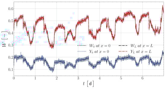
Figure 3. Distribution of experimental data $W_0$ and $W_L$ during 7 days.

The moisture at $t=0$ is interpolated from measured moisture. Thus, first-order polynomials of $x\in [0,L]$ are fitted for the length of the container.

$$\begin{array}{c}\hfill Y_i^0={\displaystyle \frac{\left(W_L^0-W_0^0\right)·x_i}{L}}+W_0^0,x_i=i\Delta x\end{array}$$

(231)

These interpolation functions are used as initial conditions for numerical solutions.

The total duration of numerical experiments is equal to the total duration of experimental data, which is a 7-day period. As a result, moisture data were calculated in dynamic behavior. Figure 3 shows moisture distribution during a 7-day period at $x=0$ and $x=L$. The residual error between the observations and the numerical results are given in Figure 4 for the moisture at different sensor locations, respectively. An error has a Gaussian symmetrical pattern around a zero value. This symmetry indicates that there is no consistent directional bias, and the model is equally likely to overestimate or underestimate the true values. In other words, this is generally a good sign for the validity of your model, as it suggests that any discrepancies between the model and reality are not systematic and could be reduced by refining the model or improving data collection methods.

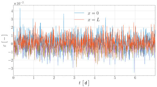
Figure 4. Error variation between the estimated and experimentally observed moisture levels $\epsilon =Y_x-W_x$ at $x=0$ and $x=L$.

The numerical outcomes from the direct problem ($Y_i^j$) are subsequently compared with the experimental data collected at $x=L$, which serve as the basis for the inverse problem. The corresponding measurements, along with their uncertainty boundaries at the sensor location ($x=L$), and the estimated values from the direct problem are depicted in Figure 3. The estimated values demonstrate a satisfactory alignment with all observation points. The deviation between numerical predictions and experimental data remains within the uncertainty range of the measurements. Finally, the model’s reliability is assessed by comparing the numerical predictions with an additional set of measurement data. Specifically, the numerical results from the direct problem ($Y_i^j$) are compared with experimental data at $x=0$, which were not used in the inverse problem resolution. Figure 3 presents the moisture comparison at $x=0$, utilizing the estimated parameters alongside experimental data at $x=L$. A highly satisfactory agreement is achieved between the numerical predictions and the experimental observations, thus confirming the reliability of the calibrated model.

The minimization of the functional continued until the relative error between the numerical solution and the experimental data reached $5.1\%$, which, in turn, shows a fairly satisfactory accuracy. Checking the absolute errors, $6.7\%$, numerical results also meet our expectations. Figure 5 illustrates the changes in parameter D during a 7-day period at points $x=10\mathrm{cm}$, $x=20\mathrm{cm}$ and $x=30\mathrm{cm}$. Despite non-smooth experimental data, the numerical results show smooth behavior, which should be investigated in future works with different data. Figure 6 demonstrates the distribution of parameter D along container lengths at times $t=2\mathrm{d}$, $t=4\mathrm{d}$ and $t=7\mathrm{d}$.

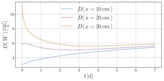
Figure 5. Distribution of D parameter during a 7-day period at $x=10\mathrm{cm}$, $x=20\mathrm{cm}$ and $x=30\mathrm{cm}$.

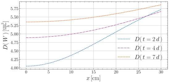
Figure 6. Distribution of D parameter along the container the container at $t=2\mathrm{d}$, $t=4\mathrm{d}$ and $t=7\mathrm{d}$.

The process of convergence of each parameter coefficient is clearly visible in Figure 7. Different initial values are chosen to verify convergence at the values.

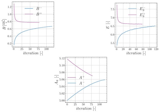
Figure 7. Convergence distribution for B, E and A parameters.

6. Conclusions

This paper presents a robust numerical method for predicting and determining moisture transfer coefficients in media with contact boundaries. In contrast to previously proposed methods, our approach simultaneously determines multiple coefficients over different time segments, taking into account the limitations of estimating multiple coefficients within a single time frame. By dividing the measured data into time segments corresponding to the number of coefficients, the numerical solution efficiently calculates each coefficient for the respective segment.

A key feature of the proposed method is its ability to solve the nonlinear moisture transfer equation with the proportionality factor coefficient D, modeled as an exponential function, and the source function $f\left(t\right)$ at the boundary, represented as a polynomial function. The inverse problem is tackled using the Conjugate Gradient method, ensuring high convergence of the solution. Initial moisture values are estimated through linear interpolation from experimental data, while the next approximation in the Conjugate Gradient method is computed using the Thomas (sweep) method, which guarantees unconditional stability.

The new results presented in this paper confirm the model’s reliability through comprehensive numerical simulations over a 7-day period. The calibration of the model using experimental data showed a discrepancy of only $5.1\%$ between experimental data and numerical estimations, which is within the uncertainty boundaries of the measurements. Additional validation using an extra measurement dataset further demonstrated that the model performs with satisfying accuracy, with the numerical results matching the experimental observations at a different location not used for the inverse problem solution.

The results also show smooth behavior in the moisture distribution across the length of the container, despite the non-smooth nature of the experimental data. This indicates the model’s robustness and suggests potential improvements through future work with different experimental datasets. The analysis of the proportionality factor D over time and across different locations within the container reveals convergent behavior, further validating the accuracy of the calibrated model.

In conclusion, the numerical method presented here proves to be a powerful tool for solving coefficient inverse problems in nonlinear moisture transfer equations. With its high accuracy, smooth numerical results, and successful validation against experimental data, the model holds promise for further applications in practical engineering tasks. Future research goals should take into account expanding the model to incorporate more complex environmental factors, such as freezing and porosity, through detailed experimental measurements.

References

- Innocenti, A.; Pazzi, V.; Napoli, M.; Ciampalini, R.; Orlandini, S.; Fanti, R. Electrical resistivity tomography: A reliable tool to monitor the efficiency of different irrigation systems in horticulture field. J. Appl. Geophys. 2024, 230, 105527. [Google Scholar] [CrossRef]
- Marcinkowski, P.; Szporak-Wasilewska, S. Assessing monthly dynamics of agricultural soil erosion risk in Poland. Geoderma Reg. 2024, 39, e00864. [Google Scholar] [CrossRef]
- El Assaad, M.; Plantec, Y.; Colinart, T.; Lecompte, T. Influence of moisture transfer on thermal conductivity measurement by HFM: Measurement accuracy on insulation materials and consequences on building energy assessments. Energy Build. 2024, 320, 114635. [Google Scholar] [CrossRef]
- Rahmat, M.N.; Ismail, N. Effect of optimum compaction moisture content formulations on the strength and durability of sustainable stabilised materials. Appl. Clay Sci. 2018, 157, 257–266. [Google Scholar] [CrossRef]
- Wu, H.; Yue, Q.; Guo, P.; Xu, X. Exploiting the potential of carbon emission reduction in cropping-livestock systems: Managing water-energy-food nexus for sustainable development. Appl. Energy 2025, 377, 124443. [Google Scholar] [CrossRef]
- Wang, W.; Ma, C.; Wang, X.; Feng, J.; Dong, L.; Kang, J.; Jin, R.; Li, X. A soil moisture experiment for validating high-resolution satellite products and monitoring irrigation at agricultural field scale. Agric. Water Manag. 2024, 304, 109071. [Google Scholar] [CrossRef]
- Vecherin, S.; Joyner, M.; Smith, M.; Linkov, I. Risk assessment of mold growth across the US due to weather variations. Build. Environ. 2024, 256, 111498. [Google Scholar] [CrossRef]
- Hu, A.; Zhou, H.; Guo, F.; Wang, Q.; Zhang, J. Three-dimensional porous fibrous structural morphology changes of high-moisture extruded soy protein under the effect of moisture content. Food Hydrocoll. 2025, 159, 110600. [Google Scholar] [CrossRef]
- Gurtin, M.; Drugan, W. An Introduction to Continuum Mechanics. J. Appl. Mech. 1984, 51, 949. [Google Scholar] [CrossRef]
- Alpar, S.; Faizulin, R.; Tokmukhamedova, F.; Daineko, Y. Applications of Symmetry-Enhanced Physics-Informed Neural Networks in High-Pressure Gas Flow Simulations in Pipelines. Symmetry 2024, 16, 538. [Google Scholar] [CrossRef]
- Leong, K.; Liu, Y. Numerical study of a combined heat and mass recovery adsorption cooling cycle. Int. J. Heat Mass Transf. 2004, 47, 4761–4770. [Google Scholar] [CrossRef]
- Gardner, D. Computer age reaches California vineyards. Irrig. Age 1983, 17, 26T–26U, 26X, 33. [Google Scholar]
- Hallaire, M.; Baldy, C. Potentiel matriciel de l’eau dans les matériaux poreux et tension superficielle de l’eau. Journées L’hydraulique 1963, 7-2, 452–458. [Google Scholar]
- Nadeem, M.; Islam, A.; Karim, S.; Mureşan, S.; Iambor, L.F. Numerical Analysis of Time-Fractional Porous Media and Heat Transfer Equations Using a Semi-Analytical Approach. Symmetry 2023, 15, 1374. [Google Scholar] [CrossRef]
- Nurtas, M.; Baishemirov, Z.; Alpar, S.; Tokmukhamedova, F. Numerical simulation of wave propagation in mixed porous media using finite element method. J. Theor. Appl. Inf. Technol. 2021, 99, 4163–4172. [Google Scholar]
- Jäger, W.; Woukeng, J.L. Homogenization of Richards’ equations in multiscale porous media with soft inclusions. J. Differ. Equ. 2021, 281, 503–549. [Google Scholar] [CrossRef]
- Foth, H. Fundamentals of Soil Science; John Wiley and Sons: New York, NY, USA, 1991. [Google Scholar]
- Chakraborty, A.; Saharia, M.; Chakma, S.; Kumar Pandey, D.; Niranjan Kumar, K.; Thakur, P.K.; Kumar, S.; Getirana, A. Improved soil moisture estimation and detection of irrigation signal by incorporating SMAP soil moisture into the Indian Land Data Assimilation System (ILDAS). J. Hydrol. 2024, 638, 131581. [Google Scholar] [CrossRef]
- Lu, Z.; Wei, J.; Yang, X. Effects of hydraulic conductivity on simulating groundwater–land surface interactions over a typical endorheic river basin. J. Hydrol. 2024, 638, 131542. [Google Scholar] [CrossRef]
- Lal, R.; Shukla, M. Principles of Soil Physics. Vadose Zone J. 2005, 4, 448. [Google Scholar]
- Nikitina, L.M. Handbook of Tables of Thermodynamic Parameters and Mass Transfer Coefficients of Wet Materials; Begell House Inc. Publishers: New York, NY, USA, 2007. [Google Scholar]
- Jones, J. Using expert systems in agricultural models. Agric. Eng. 1985, 37, 21–22. [Google Scholar]
- Alpar, S.; Rysbaiuly, B. Determination of thermophysical characteristics in a nonlinear inverse heat transfer problem. Appl. Math. Comput. 2023, 440, 127656. [Google Scholar] [CrossRef]
- Fontana, E.; Donca, R.; Mancusi, E.; de Souza, A.A.U.; de Souza, S.M.G.U. Mathematical modeling and numerical simulation of heat and moisture transfer in a porous textile medium. J. Text. Inst. 2016, 107, 672–682. [Google Scholar] [CrossRef]
- Kang, M.Z.; Cournede, P.H.; Mathieu, A.; Letort, V.; Qi, R. A Functional-Structural Plant Model-Theory and Applications in Agronomy. In Proceedings of the International Symposium on Crop Modeling and Decision Support: ISCMDS 2008, Nanjing, China, 19–22 April 2008. [Google Scholar]
- Berger, J.; Dutykh, D.; Mendes, N.; Rysbaiuly, B. A new model for simulating heat, air and moisture transport in porous building materials. Int. J. Heat Mass Transf. 2019, 134, 1041–1060. [Google Scholar] [CrossRef]
- Egusa, M.; Matsukawa, S.; Miura, C.; Nakatani, S.; Yamada, J.; Endo, T.; Ifuku, S.; Kaminaka, H. Improving nitrogen uptake efficiency by chitin nanofiber promotes growth in tomato. Int. J. Biol. Macromol. 2020, 151, 1322–1331. [Google Scholar] [CrossRef]
- Arraes, F.; Miranda, J.; Duarte, S. Modeling soil water redistribution under surface drip irrigation. Eng. Agrícola 2019, 39, 55–64. [Google Scholar] [CrossRef]
- Soares, P.R.; Pato, R.L.; Dias, S.; Santos, D. Effects of Grazing Indigenous Laying Hens on Soil Properties: Benefits and Challenges to Achieving Soil Fertility. Sustainability 2022, 14, 3407. [Google Scholar] [CrossRef]
- Chen, Y.; Ma, J.; Wu, X.; Weng, L.; Li, Y. Sedimentation and Transport of Different Soil Colloids: Effects of Goethite and Humic Acid. Water 2020, 12, 980. [Google Scholar] [CrossRef]
- Teferi, E.T.; Assefa, T.T.; Tilahun, S.A.; Wassie, S.B.; Thi Minh, T.; Béné, C. Bridging the gap: Analysis of systemic barriers to irrigation technology supply businesses in Ethiopia. Agric. Water Manag. 2024, 303, 109004. [Google Scholar] [CrossRef]
- Gomes, A.H.S.; Chaves, L.H.G.; Guerra, H.O.C. Drip irrigated sunflower Inter-cropping. Am. J. Plant Sci. 2015, 6, 1816–1821. [Google Scholar] [CrossRef][Green Version]
- Allen, R.G.; Pereira, L.S. Estimating crop coefficients from fraction of ground over and height. Irrig. Sci. 2009, 28, 17–34. [Google Scholar] [CrossRef]
- Gregory, R.H. The Handbook of Technical Irrigation Information. 2015. Available online: https://www.hunterindustries.com/sites/default/files/tech_handbook_of_technical_irrigation_information.pdf (accessed on 15 April 2024).
- Altaji, M.; Eslamian, A. Handbook of Irrigation System Selection for Semi-Arid Region; CRC Press: Boca Raton, FL, USA, 2020. [Google Scholar] [CrossRef]
- Perrier, E.; Bird, N.; Rieu, M. Generalizing the fractal model of soil structure: The pore–solid fractal approach. Geoderma 1999, 88, 137–164. [Google Scholar] [CrossRef]
- Braat, L.C.; Van Lierop, W.F. Economic-ecological modeling: An introduction to methods and applications. Ecol. Model. 1986, 31, 33–44. [Google Scholar] [CrossRef]
- Hasanov, A.; Romanov, V. Introduction to Inverse Problems for Differential Equations; Springer: Cham, Switzerland, 2017. [Google Scholar] [CrossRef]
- Hussein, S.; Lesnic, D. Determination of forcing functions in the wave equation. Part I: The space-dependent case. J. Eng. Math. 2015, 96, 115–133. [Google Scholar] [CrossRef][Green Version]
- Klibanov, M.V. Inverse problems and Carleman estimates. Inverse Probl. 1992, 8, 575. [Google Scholar] [CrossRef]
- Zhenhai, L.; Szántó, I. Inverse coefficient problems for parabolic hemivariational inequalities. Acta Math. Sci. 2011, 31, 1318–1326. [Google Scholar] [CrossRef]
- Alpar, S.; Berger, J.; Rysbaiuly, B.; Belarbi, R. Estimation of soils thermophysical characteristics in a nonlinear inverse heat transfer problem. Int. J. Heat Mass Transf. 2024, 218, 124727. [Google Scholar] [CrossRef]
- Chen, Y.; Zhang, J.H.; Chen, M.X.; Zhu, F.Y.; Song, T. Optimizing water conservation and utilization with a regulated deficit irrigation strategy in woody crops: A review. Agric. Water Manag. 2023, 289, 108523. [Google Scholar] [CrossRef]
- Rysbaiuly, B.; Ryskeldi, M.; Kul’zhanov, A.; Kalimullin, A. Sistema Nerazrushayushchego Kontrolya Harakteristik Pochvy. Technical Report, Patent na Izobretenie No2022/0596.2.2022. 2022. Available online: https://gosreestr.kazpatent.kz/Utilitymodel/Details?docNumber=359967 (accessed on 25 January 2024).
- Sánchez-Pérez, J.F.; Marín-García, F.; Castro, E.; García-Ros, G.; Conesa, M.; Solano-Ramírez, J. Methodology for Solving Engineering Problems of Burgers–Huxley Coupled with Symmetric Boundary Conditions by Means of the Network Simulation Method. Symmetry 2023, 15, 1740. [Google Scholar] [CrossRef]
- Rysbajuly, B. Obratnye Zadachi Vnelineynoy Teploprovodnosti; Kazak Universiteti: Almaty, Kazakhstan, 2022; p. 369. [Google Scholar]
- Fedotov, G. Fraktal’nye Kolloidnye Struktury v Pochvah Razlichnoii Zonal’nosti. Doklady Academii Nauk RF 2005, 405, 351–354. [Google Scholar]
Disclaimer/Publisher’s Note: The statements, opinions and data contained in all publications are solely those of the individual author(s) and contributor(s) and not of MDPI and/or the editor(s). MDPI and/or the editor(s) disclaim responsibility for any injury to people or property resulting from any ideas, methods, instructions or products referred to in the content. |
© 2024 by the authors. Licensee MDPI, Basel, Switzerland. This article is an open access article distributed under the terms and conditions of the Creative Commons Attribution (CC BY) license (https://creativecommons.org/licenses/by/4.0/).