Article

Evaluating Time Irreversibility Tests Using Geometric Brownian Motions with Stochastic Resetting

1
Instituto de Física Interdisciplinar y Sistemas Complejos CSIC-UIB, Campus Universitat de les Illes Balears, E-07122 Palma de Mallorca, Spain
2
Research Center for Computer Science and Information Technologies, Macedonian Academy of Sciences and Arts, 1000 Skopje, Macedonia
3
Institute of Physics, Faculty of Natural Sciences and Mathematics, Ss. Cyril and Methodius University, 1000 Skopje, Macedonia
4
Department of Physics, Korea University, Seoul 02841, Republic of Korea
5
Faculty of Computer Science and Engineering, Ss. Cyril and Methodius University, P.O. Box 393, 1000 Skopje, Macedonia
*
Author to whom correspondence should be addressed.
Symmetry 2024, 16(11), 1445; https://doi.org/10.3390/sym16111445
Submission received: 23 July 2024 / Revised: 2 October 2024 / Accepted: 14 October 2024 / Published: 31 October 2024
(This article belongs to the Section Physics)

Abstract

:
The time irreversibility of a dynamical process refers to the phenomenon where its behaviour or statistical properties change when it is observed under a time-reversal operation, i.e., backwards in time and indicates the presence of an “arrow of time”. It is an important feature of both synthetic and real-world systems, as it represents a macroscopic property that describes the mechanisms driving the dynamics at a microscale level and that stems from non-linearities and the presence of non-conservative forces within them. While many alternatives have been proposed in recent decades to assess this feature in experimental time series, the evaluation of their performance is hindered by the lack of benchmark time series of known reversibility. To solve this problem, we here propose and evaluate the use of a geometric Brownian motion model with stochastic resetting. We specifically use synthetic time series generated with this model to evaluate eight irreversibility tests in terms of sensitivity with respect to several characteristics, including their degree of irreversibility and length. We show how tests yield at times contradictory results, including the false detection of irreversible dynamics in time-reversible systems with a frequency higher than expected by chance and how most of them detect a multi-scale irreversibility structure that is not present in the underlying data.

1. Introduction

Time irreversibility, i.e., the lack of symmetry of a system’s dynamics under the operation of time reversal, is an important property observed in natural and synthetic processes alike. In general terms, a dynamics is considered time-irreversible whenever some of its statistical properties change when considering its time-reversed version. As a simple example, supposing a movie of an ice cube melting in a glass, and one with the ice cube forming from liquid water, an observer can easily decide which one is the original and which the time-reversed one; in this case, the creation (or destruction) of entropy is what makes the process irreversible. On the other hand, the movement of a pendulum and its time-reversed version are undistinguishable, and hence the dynamics is reversible. The history of the concept of irreversibility is a complex one, as it was initially thought to be incompatible with established physics theories—see Ref. [1] for a historical perspective.
It is rooted in thermodynamics and entails a process that cannot reverse into its initial state; for instance, the thermodynamic entropy of a thermally isolated system cannot decrease, and the latter always tends to higher disordered states. On the other hand, microscopic dynamics are usually time-reversible, as is the case of Newton’s equation of motion; hence, the irreversibility emerges only at a macro-scale level. Nowadays, the consensus is that irreversibility stems from several important properties of the system, namely non-linear dynamics; (linear or non-linear) non-Gaussian dynamics [2]; the presence of dissipative (or non-conservative) forces, i.e., forces that dissipate energy from the system, like memory or friction [3]; and the departure from equilibrium [4]. In other words, it reflects, at a macroscopic scale, important mechanisms driving the dynamics of a system at a microscopic level.
When an explicit dynamical representation of a system is not available, time irreversibility must be evaluated in experimental time series representing its evolution. Given a time series, the problem then becomes to test whenever a given property changes when considering the original and time-reversed versions of the same. Not surprisingly, many tests have hitherto been developed to assess the irreversibility of time series, thus acting as a tool to understand the underlying system—the interested reader may refer to Ref. [5] for a review. These tests perform differently depending on the characteristics of the time series under analysis [5], due to a conceptual barrier: the definition of irreversibility does not state which criteria should be used to evaluate such a lack of symmetry. Hence, different tests are based on different hypotheses that may or may not be relevant to individual cases; and this further exacerbates the problem of comparing their performance. Most importantly, this implies that the analysis of experimental time series should be performed using a battery of tests in order to avoid biased results.
In this contribution, we tackle this problem by proposing the use of a geometric Brownian motion with stochastic resetting (srGBM) [6] dynamics as a test bench for irreversibility tests. It presents the advantage of generating model time series with tuneable degrees of irreversibility and, as opposed to the model presented in Ref. [7], to the best of our knowledge, the only alternative hitherto proposed of describing a dynamics that is common in many natural and human-made systems, most notably economics [8,9,10]. In what follows, we first describe the srGBM model and discuss its irreversibility (Section 2) and introduce a suite of eight irreversibility tests commonly used in the literature (Section 3). We afterwards compare these tests using time series generated by the srGBM model under different conditions and varying the characteristics of the data (Section 4). We highlight how these tests have heterogeneous requirements in terms of, for instance, the minimum time series length required and how they yield different false positive rates, i.e., how they can detect irreversibility even in random time series that are by construction time-reversible. By changing the way the time series are generated, we also highlight how tests leverage different aspects of the dynamics, i.e., the drift or the resetting. We further show how some tests have a behaviour consistent with the presence of multi-scale irreversibility, even when such a feature is not present in the data.

2. The Geometric Brownian Motion Under Stochastic Resetting

Geometric Brownian motion (GBM) is one of the cornerstone models in the field of stochastic processes, one that has been extensively applied to describe the temporal evolution of various natural and financial systems. Its mathematical elegance and empirical relevance have made it a preferred tool for modeling phenomena ranging from stock and asset prices in financial markets [9,11,12] to the growth of social and biological populations [13,14] and the diffusion of particles in numerous physical systems [15]. However, many real-world processes are subject to occasional resets, where the system state is intermittently returned to a specific point, a feature not captured by traditional GBM. The concept of stochastic resetting has then been introduced and thoroughly investigated in recent years to address this limitation. This resetting mechanism introduces significant alterations to the dynamics of the underlying process, leading to rich and complex behaviours that are not present in the standard GBM. The combination of GBM and stochastic resetting has therefore emerged as a very robust and versatile framework, enhancing the ability to model and understand systems subject to intermittent resets. For the sake of completeness, in this section, we define the geometric Brownian motion with stochastic resetting (srGBM) model and synthesise its most important results and statistical properties. The interested reader may refer to [6] for an in-depth analysis.
The srGBM model is described by the following Langevin equation [6]:
d x ( t ) = ( 1 Z t ) x ( t ) [ δ d t + σ d W ] + Z t [ x 0 x ( t ) ] , x 0 > 0 ,
where x ( t ) is the evolution of the system with respect to time—e.g., the position of a particle, option prices, or reproducing resources such as biomass. The Wiener increment of the process d W is characterised by a zero mean d W = 0 and correlation function d W t d W s = δ ( t s ) d t . δ further denotes the drift amplitude, σ the standard deviation, and x 0 > 0 the initial value of x ( t ) , x ( 0 ) = x 0 . A resetting is introduced with a random variable Z t , which takes the value 1 when a resetting to the initial position takes place and 0 when there is no resetting. The solution of the stochastic equation in Itô interpretation is given by [6]:
x ( t ) = x 0 e [ δ ( σ 2 / 2 ) ] [ t t l ( t ) ] + σ { W ( t ) W [ t l ( t ) ] } ,
where the probability for a resetting event is given by P ( Z t = 1 ) = r d t .
It is important at this point to discuss the relevance of the srGBM model from the irreversibility viewpoint. One can start from a basic Brownian motion model, i.e., a Wiener process of independent and normally distributed increments with a zero mean. When considering the time series of increments, this is time-reversible, as the increments in the forward and time-reversed time series are drawn from the same distribution, W t + u W t = [ W t W t + u ] N ( 0 , u ) . Note that, on the other hand, Brownian motion is a diffusion process, and its dynamics (as opposed to the dynamics of increments) is hence irreversible, as its variance scales linearly with time. Next, the standard GBM model introduces non-stationarity and irreversibility, due to the drift (provided δ > 0 ) and the consequent trend in its evolution. Note that, under the time-reversal operation, the drift δ would change sign; hence an arrow of time can easily be defined. Finally, one of the key characteristics of the stochastic resetting mechanism is its ability to transform a non-stationary process into a stationary one. It is reasonable to assume that, as the resetting rate r increases, and with it the resetting probability r d t , the irreversibility of the srGBM model will progressively diminish. The rationale behind the necessity for a specific threshold of the resetting rate to achieve process reversibility lies in the probabilistic nature of the resetting events, which occur at varying values of x ( t ) . Two values, x i ( t i ) and x i + 1 ( t i + 1 ) , for two consecutive resetting events, can differ significantly from one from another, meaning the trajectory of the microstate does not have the same likelihood of occurring as its time-reverse counterpart. However, with higher resetting probabilities r d t , these coordinates for the resetting events become more similar, thereby enhancing the process’s reversibility. Full reversibility is achieved when the resetting probability reaches 1. This phenomenon is illustrated through simulations of the GBM with stochastic resetting (srGBM) for different resetting probabilities, as depicted in the top panel of Figure 1. On the other hand, the drift δ is expected to generate the opposite effect. Specifically, larger drifts will result in greater irreversibilities of the process. Conversely, for δ = 0 , the initial time series are stationary, and the stochastic resetting process may make them irreversible through a process known as thermalisation [16]. It is thus evident that both the resetting rate and the drift can be used to tune the degree of irreversibility in the observed system.
As a final note, and unless otherwise specified, time series have here been generated using the srGBM with standard parameters δ = 10 2.5 , r = 0.01 , σ = 0.01 , x 0 = 1 , and l = 10 3 (where l is the length of the time series). Additionally, in all cases, d t = 1 (and hence r d t = r ), in order to obtain time series resembling experimental ones and that can directly be analysed by the tests.

3. Tests for Time Irreversibility

As previously introduced, multiple numerical tests have been proposed in recent decades to detect time irreversibility in experimental time series, each one based on different hypotheses and hence capturing different properties of the data. In what follows, we provide a short review of the eight methods considered in this study, alongside relevant references and the combinations of parameters used here—see also Table 1 for a synthesis. The interested reader can refer to Ref. [5] for further details. In all cases, the software implementation corresponds to the library included in the previous review, and freely available at https://gitlab.com/MZanin/irreversibilitytestslibrary (accessed on 1 July 2024).
  • Pomeau’s test. To the best of our knowledge, this test was the first one ever proposed for the study of real-world time series. It is based on the evaluation of a function asymmetric with respect to time:
    ϕ ( τ ) = x ( t ) [ x ( t + 2 τ ) x ( t + τ ) ] x ( t + 3 τ ) ¯ ,
    with τ being a lag constant [17]. ϕ ( τ ) is then compared against the values obtained for a large set of randomly shuffled time series, in order to extract a p-value. We here consider τ = 1 , 2 , 3 .
  • Diks’ test. The second numerical test to be proposed to detect irreversibility in data, it is based on extracting vectors representing subsets of the original time series, e.g., non-overlapping sub-windows with embedding dimension m and embedding delay τ , and on estimating the distance between these and their time-reversed counterpart through an unbiased estimator under the null hypothesis of independence [18]. We here use m = 4 , 6 , 8 and τ = 1 .
  • BDS statistics. Initially proposed by Broock, Dechert and Scheinkman as a test to check for the presence of low-dimensional chaos in economic and financial data [19,20], it was later used also for the detection of irreversibility. Given a time series x ( t ) composed of T observations, the statistic is defined as
    w d ( r , T ) = T C m ( r , T ) C 1 ( r , T ) m σ m ( r , T ) ,
    with C m ( r , T ) being the sample correlation integral at embedding dimension m and scaling parameter r and σ m ( r , T ) the estimated standard deviation of the statistic under the null hypothesis of independence. Under the null hypothesis of independent (and hence, time symmetrical) data, w d is distributed asymptotically as N ( 0 , 1 ) . We here consider the standard value m = 2 .
  • Visibility Graphs. A recently proposed family of approaches to analyse time series is the one based on representing these as complex networks [21,22], whose nodes correspond to the individual data points, and pairs of nodes are connected when they fulfil some geometrical rule. We here consider the so-called directed Horizontal Visibility Graphs (dHVGs) as a representative of this family, in which pairs of nodes are connected if the line joining the corresponding values is not obstructed by another intermediate point, or, in other words, if these nodes can “see” each other [23]. A time series is then reversible if the distributions of in- and out-degrees (i.e., respectively, the number of links arriving to and departing from a given node) are the same according to an Epps–Singleton test [24].
  • Permutation pattern test. Independently proposed by several groups [25,26,27,28], these tests are based on representing the time series as sequences of permutation patterns, i.e., (usually short) patterns describing the order that has to be applied to sort them in increasing order [29], for then comparing the distributions obtained in the original and time-reversed versions. We here consider embedding dimensions of D = [ 3 , 4 , 5 ] and compare the frequency of appearance of time-symmetric patterns using a binomial test as suggested in Ref. [25].
  • Ternary Coding test. Conceptually similar to the previous one, the Ternary Coding test is based on the idea of representing a time series as a sequence of symbols and then evaluating the difference in their frequency under a time-reversal operation [30]. Specifically, a time series x ( t ) is firstly differentiated as d ( t ) = x ( t + 1 ) x ( t ) and secondly transformed according to
    s ( t ) = 1 , if d ( t ) > α 1 , if d ( t ) < α 0 , otherwise .
    The full test is constructed by splitting the time series s ( t ) into D non-overlapping segments and evaluating if the difference in the frequency of the three symbols is statistically significant. We here consider D = 10 , 20 , 40 , 80 .
  • Costa index. Costa and coauthors proposed this test in the context of the study of heartbeat dynamics [31], and it involves comparing the number of times the time series increases or decreases—i.e., x ( t ) > x ( t + 1 ) vs. x ( t ) < x ( t + 1 ) . A p-value is further calculated by comparing such asymmetry with the one obtained in randomly shuffled time series.
  • Continuous Ordinal Patterns (COPs). Continuous Ordinal Patterns elaborate on the idea of permutation patterns previously introduced and are based on fixing a short pattern of size D for a whole time series and calculating the distance of each sub-window in the original time series to such a reference pattern [32]. In other words, the original time series is transformed into a new one measuring how well the COP under study describes it through time. An irreversibility metric can then be constructed by finding the COP maximising the distance between the original and the time-reversed time series, the distance being evaluated through a two-sample Kolmogorov–Smirnov test. We here consider D = 3 , 4 , 5 , 6 .
Table 1. Numerical tests for detecting time irreversibility in time series, grouped into global families. The last column reports the combinations of parameters considered in this study, with the default one marked in bold.
Metric FamilyMetricsReferenceParameters
Classical time series analysisPomeau’s test [17] τ = 1 , 2 , 3
Diks’ test [18] m = 4 , 6 , 8 ; τ = 1
BDS Statistics [19,20] m = 2
Network-basedVisibility Graphs [23]-
Symbolic analysisPermutation patterns test [25] D = 3 , 4 , 5
Ternary Coding test [30] D = 10 , 20 , 40 , 80
OthersCosta index [31]-
Continuous Ordinal Patterns [32] D = 3 , 4 , 5 , 6

4. Results

4.1. Main Model Parameters

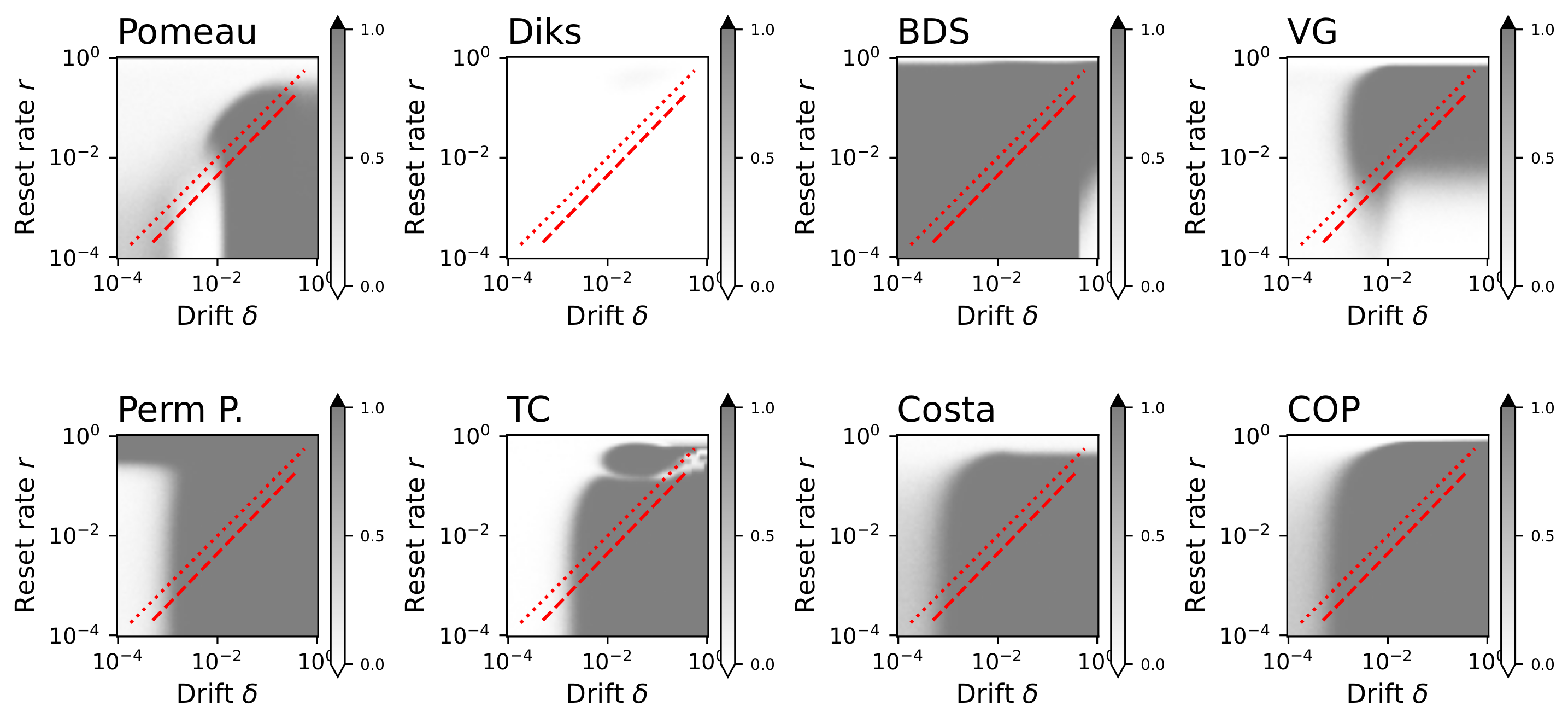
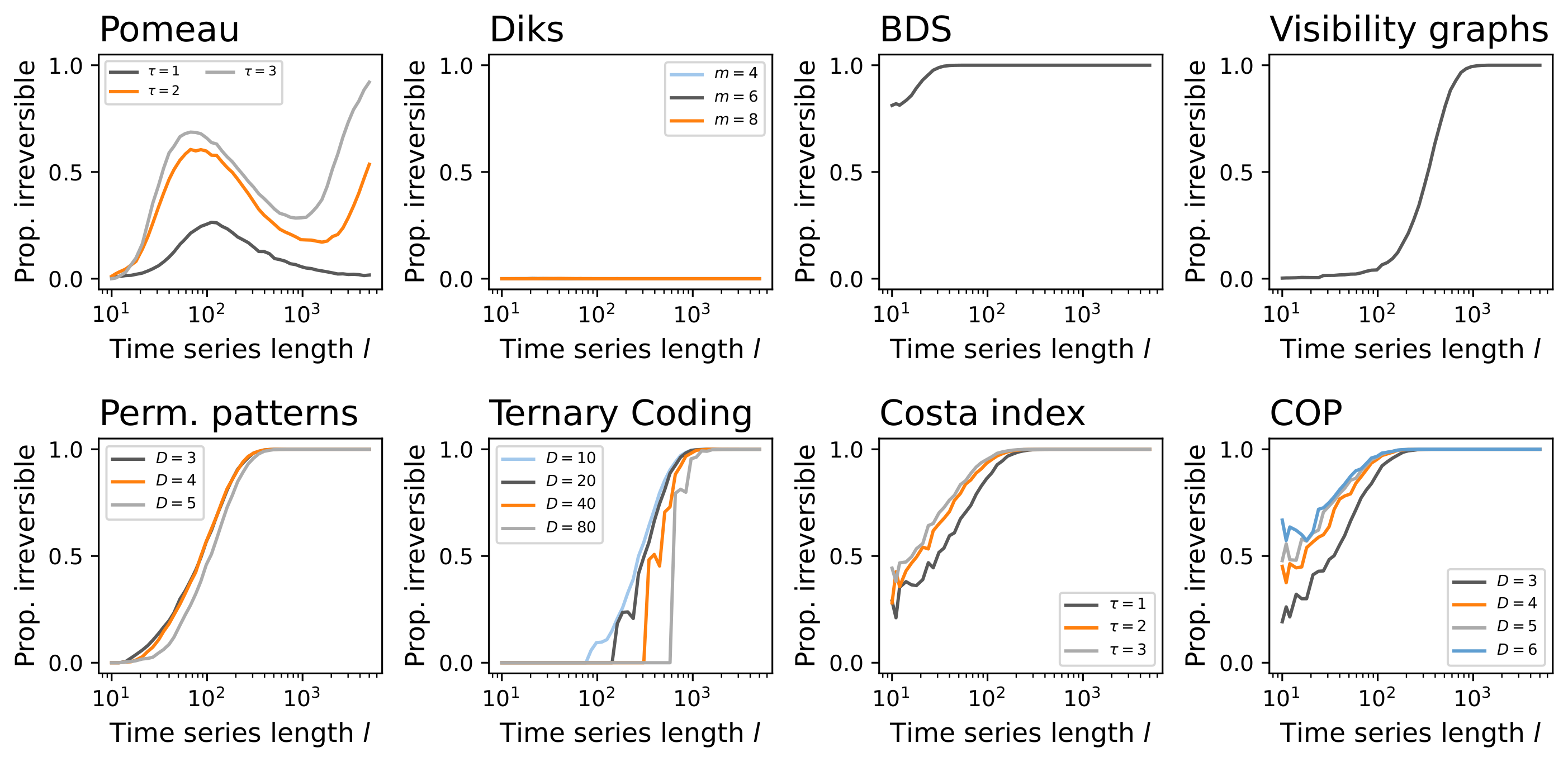
We start the analysis by evaluating the effectiveness of each irreversibility test as a function of the three main parameters of the srGBM model. Specifically, Figure 2 and Figure 3 report the performance of each test as a function, respectively, of the drift δ and the reset probability r, and of the length of the time series l. In what follows, such performance is evaluated by executing each test over 10 4 independent time series, and by calculating the fraction of times (also denoted as the proportion of irreversible time series, or “Prop. irreversible” in the figures), each test yields a statistically significant result (for α = 0.01 ). In other words, this fraction refers to the proportion of instances or trials in which a given method or test successfully identifies a stochastic process as being time-irreversible. It is a statistical measure often used in studies that involve multiple time-series datasets or simulations to evaluate the effectiveness of irreversibility detection methods. For example, if 10 4 time series are analysed using a specific test for irreversibility, and the test identifies 700 of them as irreversible (with a p-value smaller than 0.01 ), this fraction would be 70 % (or 0.7 ). Note that, in theory, given a dynamical system, time series generated by it should either be all time-reversible or irreversible—i.e., the corresponding fraction of irreversible time series should be either zero or one. Yet, due to the stochastic nature of the time series generation process, intermediate results can be obtained. Hence, this metric is useful for comparing the sensitivity of different irreversibility detection methods across varying conditions or datasets.
As is to be expected, tests generally perform better with larger drifts, smaller reset probabilities, and longer time series. There are nevertheless some interesting behaviours; for instance, some tests consistently underperform, the most notable case being Diks’ test—note that the average fraction of time series detected as irreversible is below 1 % , hence the white colour.
It is quite surprising to see that the behaviour of some tests is not monotonous with respect to the evolution of some parameters. To illustrate, the VG test yields a low proportion of significant results for r < 10 2 and δ > 10 2 , a region that presents no challenge for other methods (see the bottom right part of the panel). Pomeau’s test has a local minimum for r 10 2 , and it further improves with medium and extremely long time series—see Figure 3—a dynamics that is unique to this test. Additionally, the TC test also presents a unique local minimum for a narrow region around r = 10 1 . Their results highlight a main message already highlighted in the literature: while trying to quantify the same property, the different approaches taken by each test can lead to heterogeneous (and at times, contradictory) results.
The dashed and dotted red lines in Figure 2, respectively, correspond to r = δ and r = 2 δ + σ 2 . These are relevant as they divide the parameter space in three regions with a different dynamics: from top to bottom in each panel, a convergent, a linear divergent, and an exponential divergent behaviour. In the former case, i.e., above the dotted lines and for r > 2 δ + σ 2 , the sample average resembles the ensemble value, thus leading to ergodicity—see Ref. [6] for a demonstration. From the results presented here, it is nevertheless clear that ergodicity does not imply time-reversibility, at least according to the tests considered here.
A final interesting result is yielded by the permutation pattern test and specifically the fact that it detects as irreversible time series for very small drift and high reset rates. Note that this goes against the initial intuition, as δ < 10 4 implies that the initial time series are time-reversible. This may nevertheless be the result of a process of thermalisation: initially time-reversible time series are made irreversible by a stochastic process, which occurs when the system loses memory of its history without the necessity of energy dissipation—see Ref. [16] for an in-depth review. Notably, the same process is not detected by any other test, including the COP one—which shares some conceptual commonalities with it.

4.2. Noisy Dynamics and False Positives

An additional parameter of the srGBM model that was previously not analysed is Wiener’s deviation σ , which can be seen as the amplitude of an internal noise in the evolution of the model. In a complementary way, one can also consider an external observational noise, which is here simulated through the addition to the generated time series of random values drawn from a normal distribution N ( 0 , ξ ) . The behaviour of six tests is depicted in Figure 4 as a function of σ (left panel) and of ξ (right panel); note that the Diks and BDS tests are not reported here, as they always yield, respectively, very large and very small p-values. Results are as expected, with both internal and external noise negatively affecting the detection of irreversibility and with the Costa index and the COP test being the most resilient.
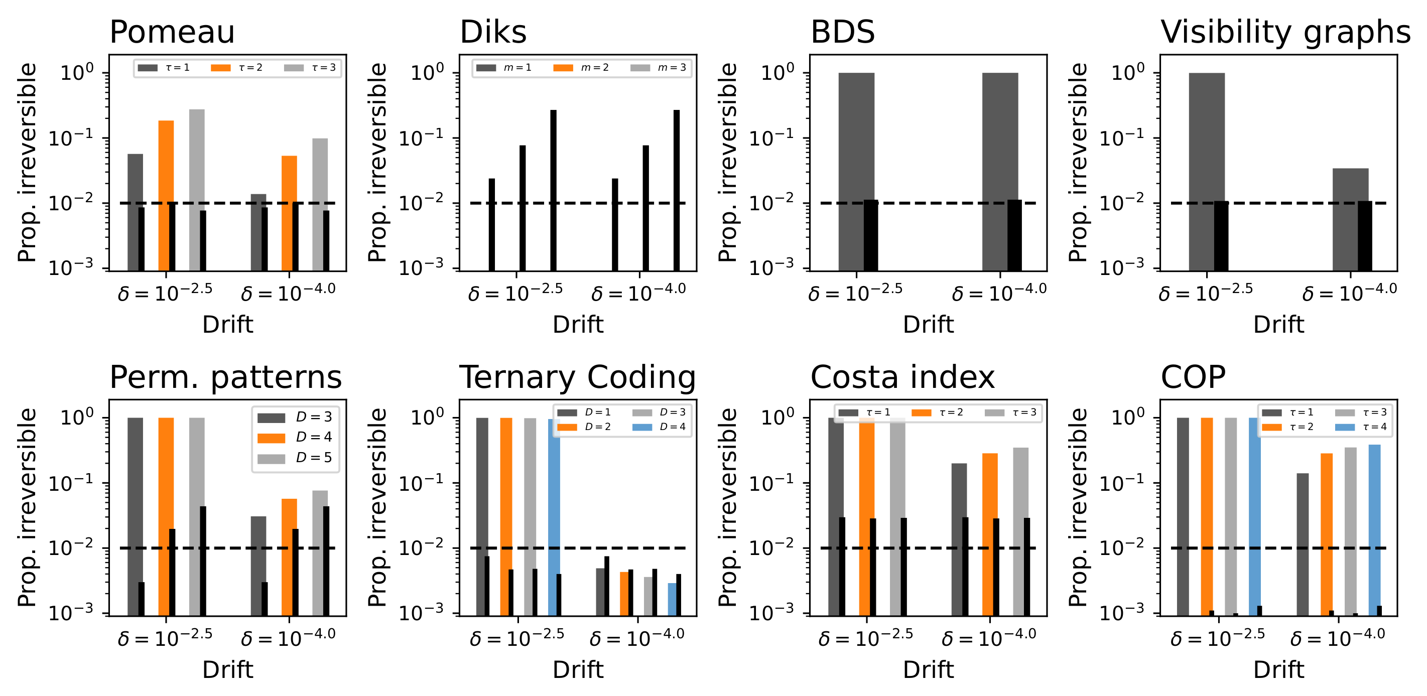
We next analyse the behaviour of the tests in terms of false positives. Specifically, we generated time series using the srGBM model and then randomly shuffling them, thus deleting any temporal structure—consequently making them time-reversible. The thin black bars in each panel of Figure 5 report the fraction of these time series that are detected as irreversible. As a reference, the horizontal dashed lines indicate a 0.01 probability, i.e., the level consistent with a significance level of α = 0.01 , and the thick coloured bars represent the corresponding proportion detected in the raw time series. All tests behave as expected, with the exception of Diks’ and Costa’s tests, which yield a higher number of false positives than expected.

4.3. Multi-Scale

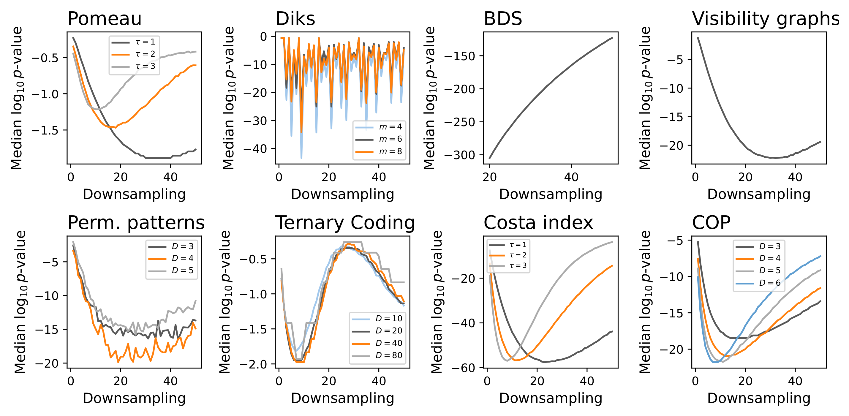
We further evaluate how the different tests behave in a multi-scale context, i.e., when only one in every n values of the original srGBM time series are considered in the analysis. The results, in terms of the median log 10 of the p-values obtained by each test and as a function of the downsampling rate, are presented in Figure 6—note that the p-value, instead of the proportion of irreversible time series, is here used to allow the comparison between strongly different results. It is interesting to observe that all tests, with the only exception being the BDS one, benefit from a downsampling of the time series. Furthermore, the presence of clear local minima in the evolution of the p-value as a function of the downsampling rate n suggests that the different methods are detecting characteristic time scales in the irreversibility, which are nevertheless not present in the original model. In other words, while seven out of eight methods report the presence of a multi-scale irreversibility, this is only an artefact of the methods themselves. This result will be further discussed below.

4.4. What Are Irreversibility Tests Detecting?

As a last point, we are going to explore one final question that is usually neglected when proposing new time irreversibility tests but that can be tackled using the srGBM model: what are these tests actually detecting? Specifically, the srGBM model provides two complementary ways for generating irreversibility, namely the drift and the stochastic reset. Notably, these two mechanisms are conceptually different and antagonistic: while the drift makes the time series non-stationary and hence irreversible, the stochastic reset deletes the memory and makes it ergodic.
The competition between these two mechanisms can be controlled by modifying the srGBM model and by generating time series including a fixed number of resets randomly located throughout the time series, as opposed to fixing a probability. We then analyse the behaviour of the Pomeau and VG tests as a function of the number of resets. These two tests have been selected for presenting almost opposite behaviours, especially for small values of r and for intermediate values of δ —see for instance r 10 3 and δ 10 2 in Figure 2.
As can be seen in Figure 7, Pomeau’s test works better when no resets are included; on the contrary, the Visibility Graph benefits from multiple resets, independently of the length of the time series. In other words, the former is more sensitive to the presence of a drift in the time series, while the latter is mainly sensitive to the resets as fingerprints of irreversibility. This suggests the possibility of comparing the results of multiple tests as a way of probing the mechanisms underpinning the observed irreversibility.

5. Discussion and Conclusions

In this contribution, we have explored the use of a geometric Brownian motion model with stochastic resetting (srGBM) as a tool to evaluate the performance of a large set of tests designed to detect the time irreversibility of real-world time series. In spite of the interest of the scientific community in the concept of irreversibility, especially in the context of the analysis of experimental time series, to the best of our knowledge, only one alternative synthetic model has been proposed for this objective [7], and usually, the evaluation relies on chaotic maps of known properties [5]. Beyond having a tuneable irreversibility, the srGBM presents the advantage of being a model of the dynamics observed in many real-world systems and is especially relevant in economics [9,11,12].
The results presented here highlight a large variability in the performance and the requirements of each method. The higher sensitivity is obtained by the BDS method when tuning both the drift and the reset probability in the model—see Figure 2. It is nevertheless worth noting that the BDS test is not only assessing irreversibility but was instead initially introduced as a test for low-dimensional chaos [19,20]; hence, results may be biased by other properties of the time series. Beyond BDS, the best methods seem to be the Costa index [31] and the COP test [32], which are both highly sensitive to the two aforementioned parameters and requiring shorter time series (see Figure 3). The nature of the srGBM model further allows one to partially probe the characteristics of the time series used by each test to detect irreversibility and specifically the competition between the drift and the stochastic reset. This could in principle be used to combine multiple tests together and obtain information about what makes a time series irreversible.
It is further interesting to note some counterintuitive behaviours of these tests. For example, the Pomeau’s test performs better with medium-length time series (approx. 100 points; see Figure 3), yet, for τ = 1 , its performance drops with more data. Secondly, Diks’ test, beyond underperforming in general, yields a significant proportion of false positives when used on a randomly shuffled version of the original time series—see Figure 5. Thirdly, and most notably, with the exception of the BDS test, all other approaches detected a multi-scale irreversibility structure that is not present in the data and that therefore emerges as an artefact of the analysis. This raises an important flag in the analysis of experimental data: a drop in the p-value yielded by a test under a downsampling procedure must not directly be interpreted as the presence of a multi-scale irreversibility.

Author Contributions

Conceptualisation, M.Z.; methodology, M.Z. and P.T.; software, M.Z. and P.J.; formal analysis, all authors; writing—original draft preparation, all authors; writing—review and editing, all authors; supervision, M.Z. and L.K. All authors have read and agreed to the published version of the manuscript.

Funding

Grant CNS2023-144775 funded by MICIU/AEI/10.13039/501100011033 by “European Union NextGenerationEU/PRTR”. This project has received funding from the European Research Council (ERC) under the European Union’s Horizon 2020 research and innovation programme (Grant Agreement No. 851255). This work has been partially supported by the María de Maeztu project CEX2021-001164-M funded by the MCIN/AEI/10.13039/501100011033. P.T., P.J., T.S. and L.K. acknowledge financial support by the German Science Foundation (DFG, Grant number ME 1535/12-1) and by the Alliance of International Science Organizations (Project No. ANSO-CR-PP-2022-05).

Data Availability Statement

Data are contained within the article.

Conflicts of Interest

The authors declare no conflicts of interest. The funders had no role in the design of the study; in the collection, analyses, or interpretation of data; in the writing of the manuscript; or in the decision to publish the results.

Abbreviations

srGBMGeometric Brownian motion with stochastic resetting
BDSBroock, Dechert and Scheinkman
VGVisibility Graph
dHVGDirected Horizontal Visibility Graph
COPContinuous Ordinal Patterns

References

  1. Hollinger, H.B.; Zenzen, M. The Nature of Irreversibility: A Study of Its Dynamics and Physical Origins; Springer Science & Business Media: Dordrecht, The Netherlands, 2012; Volume 28. [Google Scholar]
  2. Weiss, G. Time-reversibility of linear stochastic processes. J. Appl. Probab. 1975, 12, 831–836. [Google Scholar] [CrossRef]
  3. Puglisi, A.; Villamaina, D. Irreversible effects of memory. Europhys. Lett. 2009, 88, 30004. [Google Scholar] [CrossRef]
  4. Fodor, É.; Nardini, C.; Cates, M.E.; Tailleur, J.; Visco, P.; Van Wijland, F. How far from equilibrium is active matter? Phys. Rev. Lett. 2016, 117, 038103. [Google Scholar] [CrossRef] [PubMed]
  5. Zanin, M.; Papo, D. Algorithmic approaches for assessing irreversibility in time series: Review and comparison. Entropy 2021, 23, 1474. [Google Scholar] [CrossRef]
  6. Stojkoski, V.; Sandev, T.; Kocarev, L.; Pal, A. Geometric Brownian motion under stochastic resetting: A stationary yet nonergodic process. Phys. Rev. E 2021, 104, 014121. [Google Scholar] [CrossRef]
  7. Burykin, A.; Costa, M.D.; Peng, C.K.; Goldberger, A.L.; Buchman, T.G. Generating signals with multiscale time irreversibility: The asymmetric weierstrass function. Complexity 2011, 16, 29–38. [Google Scholar] [CrossRef]
  8. Nirei, M.; Souma, W. Income distribution and stochastic multiplicative process with reset event. In The Complex Dynamics of Economic Interaction: Essays in Economics and Econophysics; Springer: Berlin/Heidelberg, Germany, 2004; pp. 161–168. [Google Scholar]
  9. Stojkoski, V.; Sandev, T.; Basnarkov, L.; Kocarev, L.; Metzler, R. Generalised geometric Brownian motion: Theory and applications to option pricing. Entropy 2020, 22, 1432. [Google Scholar] [CrossRef]
  10. Stojkoski, V.; Jolakoski, P.; Pal, A.; Sandev, T.; Kocarev, L.; Metzler, R. Income inequality and mobility in geometric Brownian motion with stochastic resetting: Theoretical results and empirical evidence of non-ergodicity. Philos. Trans. R. Soc. A 2022, 380, 20210157. [Google Scholar] [CrossRef]
  11. Gerber, H.U.; Shiu, E.S. Geometric Brownian motion models for assets and liabilities: From pension funding to optimal dividends. N. Am. Actuar. J. 2003, 7, 37–51. [Google Scholar] [CrossRef]
  12. Reddy, K.; Clinton, V. Simulating stock prices using geometric Brownian motion: Evidence from Australian companies. Australas. Account. Bus. Financ. J. 2016, 10, 23–47. [Google Scholar]
  13. Damos, P.; Rigas, A.; Savopoulou-Soultani, M. Application of Markov Chains and Brownian Motion Models on Insect Ecology; Nova Science Publishers: Hauppauge, NY, USA, 2011; pp. 71–104. [Google Scholar]
  14. Jin, F.; Khandpur, R.P.; Self, N.; Dougherty, E.; Guo, S.; Chen, F.; Prakash, B.A.; Ramakrishnan, N. Modeling mass protest adoption in social network communities using geometric brownian motion. In Proceedings of the 20th ACM SIGKDD International Conference on Knowledge Discovery and Data Mining, New York, NY, USA, 24–27 August 2014; pp. 1660–1669. [Google Scholar]
  15. Engen, S. Stochastic growth and extinction in a spatial geometric Brownian population model with migration and correlated noise. Math. Biosci. 2007, 209, 240–255. [Google Scholar] [CrossRef] [PubMed]
  16. Roduner, E.; Krüger, T.P. The origin of irreversibility and thermalization in thermodynamic processes. Phys. Rep. 2022, 944, 1–43. [Google Scholar] [CrossRef]
  17. Pomeau, Y. Symétrie des fluctuations dans le renversement du temps. J. Phys. 1982, 43, 859–867. [Google Scholar] [CrossRef]
  18. Diks, C.; Van Houwelingen, J.; Takens, F.; DeGoede, J. Reversibility as a criterion for discriminating time series. Phys. Lett. A 1995, 201, 221–228. [Google Scholar] [CrossRef]
  19. Brock, W.A.; Hsieh, D.A.; LeBaron, B.D. Nonlinear Dynamics, Chaos, and Instability: Statistical Theory and Economic Evidence; MIT Press: Cambridge, MA, USA, 1991. [Google Scholar]
  20. Rothman, P. The comparative power of the TR test against simple threshold models. J. Appl. Econom. 1992, 7, S187–S195. [Google Scholar] [CrossRef]
  21. Strogatz, S.H. Exploring complex networks. Nature 2001, 410, 268–276. [Google Scholar] [CrossRef]
  22. Boccaletti, S.; Latora, V.; Moreno, Y.; Chavez, M.; Hwang, D.U. Complex networks: Structure and dynamics. Phys. Rep. 2006, 424, 175–308. [Google Scholar] [CrossRef]
  23. Lacasa, L.; Nunez, A.; Roldán, É.; Parrondo, J.M.; Luque, B. Time series irreversibility: A visibility graph approach. Eur. Phys. J. B 2012, 85, 1–11. [Google Scholar] [CrossRef]
  24. Epps, T.; Singleton, K.J. An omnibus test for the two-sample problem using the empirical characteristic function. J. Stat. Comput. Simul. 1986, 26, 177–203. [Google Scholar] [CrossRef]
  25. Zanin, M.; Rodríguez-González, A.; Menasalvas Ruiz, E.; Papo, D. Assessing time series reversibility through permutation patterns. Entropy 2018, 20, 665. [Google Scholar] [CrossRef]
  26. Martínez, J.H.; Herrera-Diestra, J.L.; Chavez, M. Detection of time reversibility in time series by ordinal patterns analysis. Chaos Interdiscip. J. Nonlinear Sci. 2018, 28, 123111. [Google Scholar] [CrossRef] [PubMed]
  27. Li, J.; Shang, P.; Zhang, X. Time series irreversibility analysis using Jensen–Shannon divergence calculated by permutation pattern. Nonlinear Dyn. 2019, 96, 2637–2652. [Google Scholar] [CrossRef]
  28. Zunino, L.; Olivares, F.; Ribeiro, H.V.; Rosso, O.A. Permutation Jensen-Shannon distance: A versatile and fast symbolic tool for complex time-series analysis. Phys. Rev. E 2022, 105, 045310. [Google Scholar] [CrossRef] [PubMed]
  29. Bandt, C.; Pompe, B. Permutation entropy: A natural complexity measure for time series. Phys. Rev. Lett. 2002, 88, 174102. [Google Scholar] [CrossRef] [PubMed]
  30. Cammarota, C.; Rogora, E. Time reversal, symbolic series and irreversibility of human heartbeat. Chaos Solitons Fractals 2007, 32, 1649–1654. [Google Scholar] [CrossRef]
  31. Costa, M.; Goldberger, A.L.; Peng, C.K. Broken asymmetry of the human heartbeat: Loss of time irreversibility in aging and disease. Phys. Rev. Lett. 2005, 95, 198102. [Google Scholar] [CrossRef]
  32. Zanin, M. Continuous ordinal patterns: Creating a bridge between ordinal analysis and deep learning. Chaos Interdiscip. J. Nonlinear Sci. 2023, 33, 033114. [Google Scholar] [CrossRef]
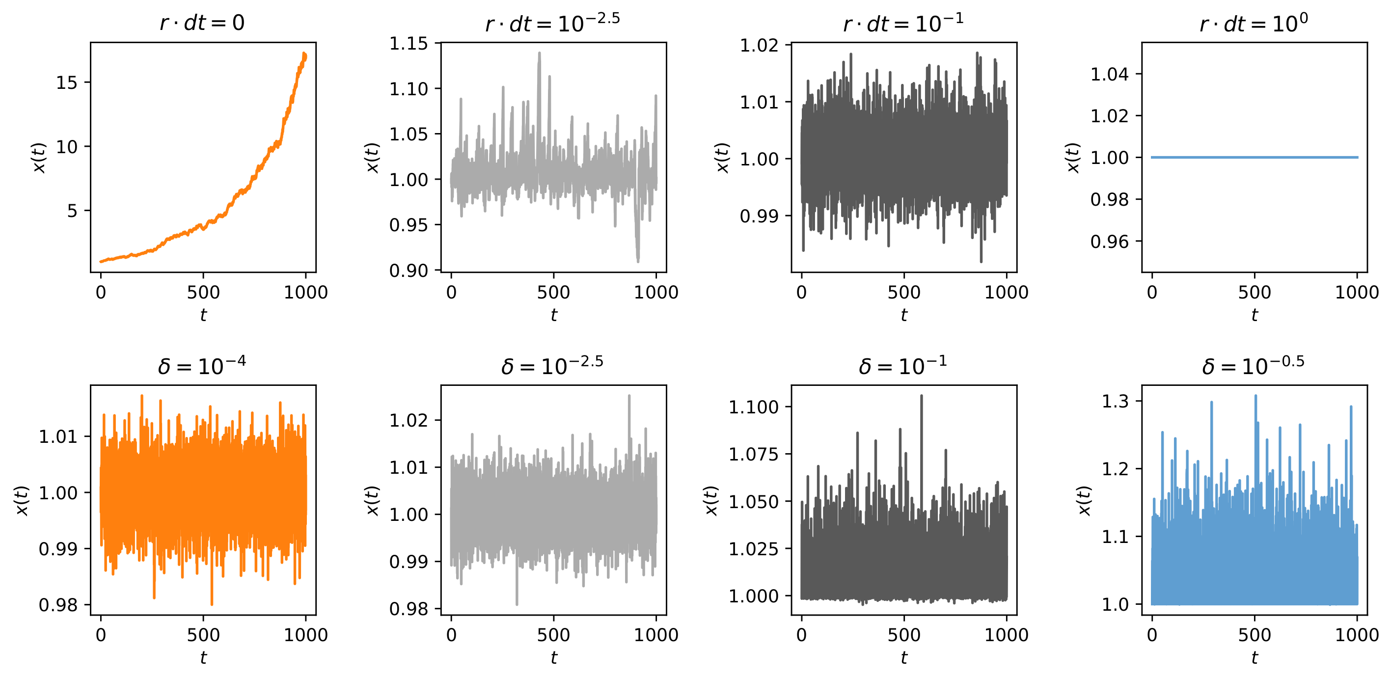
Figure 1. Examples of trajectories generated with the srGBM model. Top panel: trajectories for different resetting probabilities with drift δ = 10 2.5 . Bottom panel: trajectories for different values of the drift ( δ ) with resetting probability r d t = 0.1 . In all cases, σ = 0.01 , x 0 = 1 , T = 1000 , d t = 0.01 .
Symmetry 16 01445 g001
Figure 2. Fraction of time series detected as irreversible, by each test, as a function of the drift δ and the reset rate r. Dashed and dotted red lines, respectively, correspond to r = δ and r = 2 δ + σ 2 . The parameters used in each test correspond to the standard ones (marked in bold in Table 1). In all cases, l = 1000 .
Symmetry 16 01445 g002
Figure 3. Fraction of time series detected as irreversible, by each test, as a function of the time series length l. Each panel corresponds to a test, while different lines indicate the results for different parameter values of the same (see legends). In all cases, δ = 10 2.5 and r = 0.01 .
Symmetry 16 01445 g003
Figure 4. Behaviour of the irreversibility tests in the presence of noise. Each panel represents the evolution of the median of the log 10 of the p-value yielded by each test, as a function of the internal ( σ , left panel) and the external ( ξ , right panel) noise amplitude. In all cases, δ = 10 2.5 , r = 0.01 , and l = 10 3 .
Symmetry 16 01445 g004
Figure 5. Behaviour of the eight tests in terms of false positives. The thin black bars report the proportion of time series that are detected as irreversible when they are randomly shuffled to destroy any temporal structure. The coloured bars report the same metric on the original time series. The horizontal dashed lines indicate the value compatible with a significance level of α = 0.01 .
Symmetry 16 01445 g005
Figure 6. Evolution of the median of the log 10 p -value, as obtained by each test as a function of the downsampling rate of the time series. In all cases, δ = 10 3 , r = 0.01 and l = 1000 .
Symmetry 16 01445 g006
Figure 7. Fraction of time series detected as irreversible, the Pomeau’s (left panel) and the Visibility Graph test (right panel), as a function of the time series length l and for different numbers of resets ( n r ; see legends). δ = 10 2.5 in both cases.
Symmetry 16 01445 g007
Disclaimer/Publisher’s Note: The statements, opinions and data contained in all publications are solely those of the individual author(s) and contributor(s) and not of MDPI and/or the editor(s). MDPI and/or the editor(s) disclaim responsibility for any injury to people or property resulting from any ideas, methods, instructions or products referred to in the content.