

Differential Evolution Using Enhanced Mutation Strategy Based on Random Neighbor Selection

 , , , and
Abstract
:1. Introduction
1.1. Problem Statement
| Algorithm 1: Improved Random Neighbor-Based Differential Evolution |
|
1.2. Research Significance
1.3. Research Contributions
- This paper presents a novel mutation strategy in the RNDE algorithm to maintain the balance between the exploration and exploitation of the DE algorithm. The proposed IRNDE is helpful in increasing the convergence speed and average fitness solution quality of results.
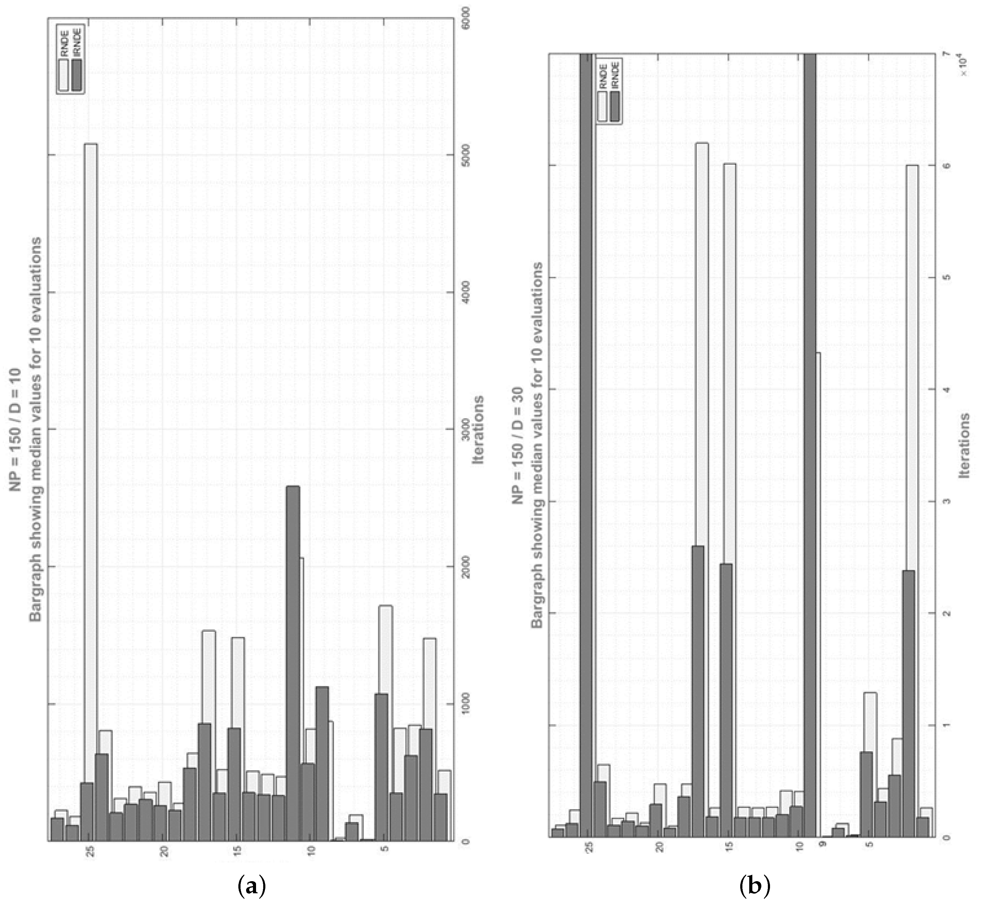
- Experimental results show that the performance of the improved RNDE algorithm is superior, as compared to the RNDE algorithm for the standard test suit of benchmark functions.
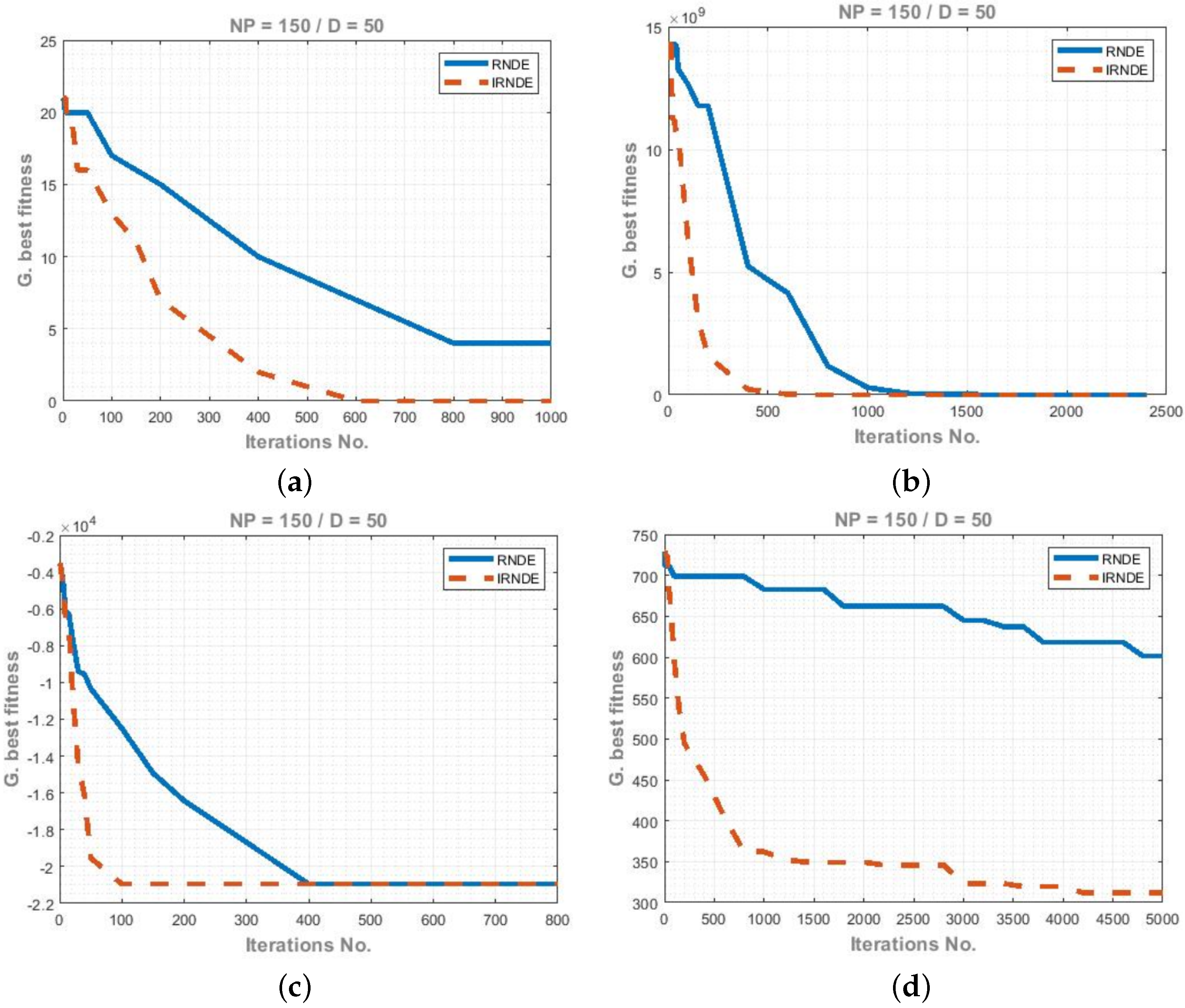
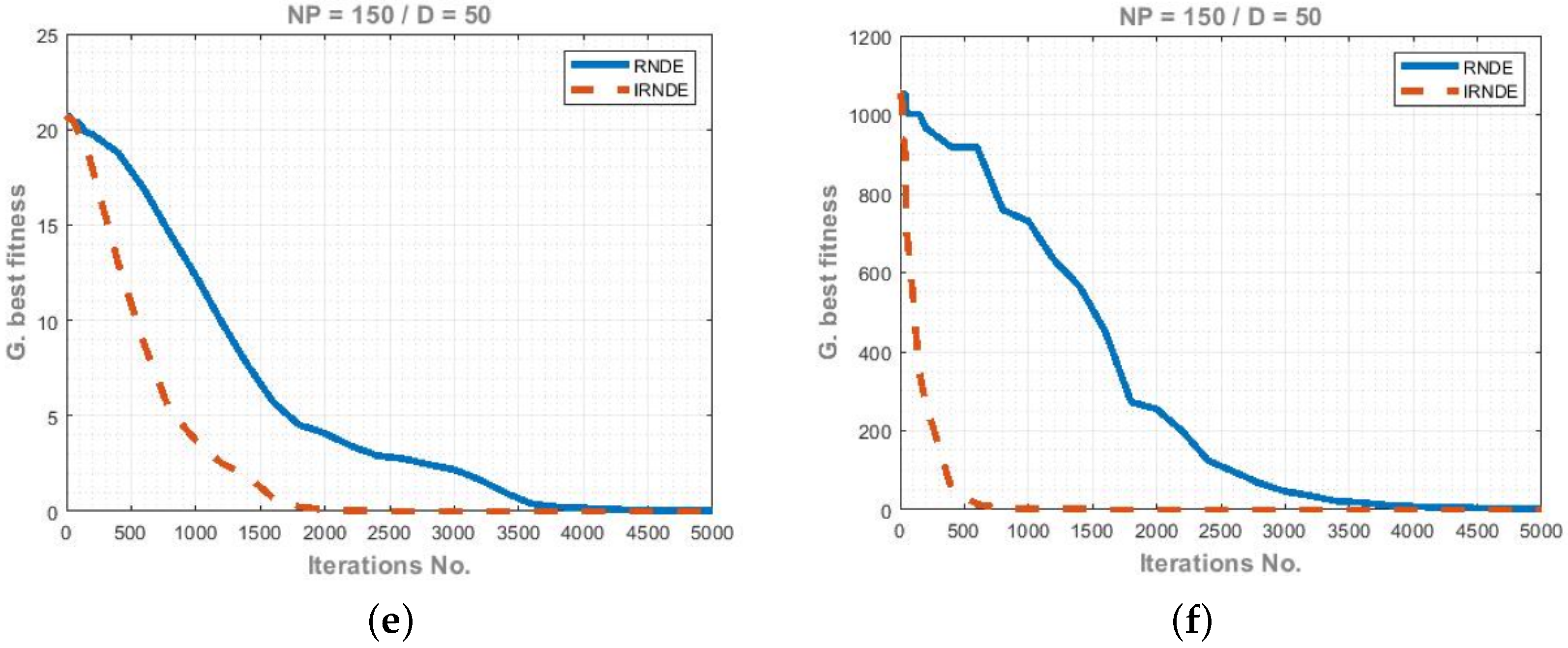
- Convergence graphs confirm the quick convergence of the proposed IRNDE algorithm and statistical results show the significance of the IRNDE algorithm.
1.4. Research Question and Hypothesis
- Ways to increase population diversity and incorporate a balance between exploration and exploration during the evolution process of the RNDE algorithm.
- Finding significance in the performance of the RNDE algorithm and proposed algorithm.
2. Principle of the Classical Differential Evolution Algorithm
2.1. Mutation Phase
2.2. Crossover Phase
2.3. Selection Phase
2.4. Commonly Used Mutation Strategies
2.5. Major Contributions of Study
3. Related Work
3.1. Hybridization with Other Techniques
3.2. Modification of Mutation Strategies
3.3. Adaptation of Mutation Strategy and Parameter Settings
3.4. Use of Neighbor Information
4. Materials and Methods
4.1. DE with Random Neighbor-Based Mutation Strategy
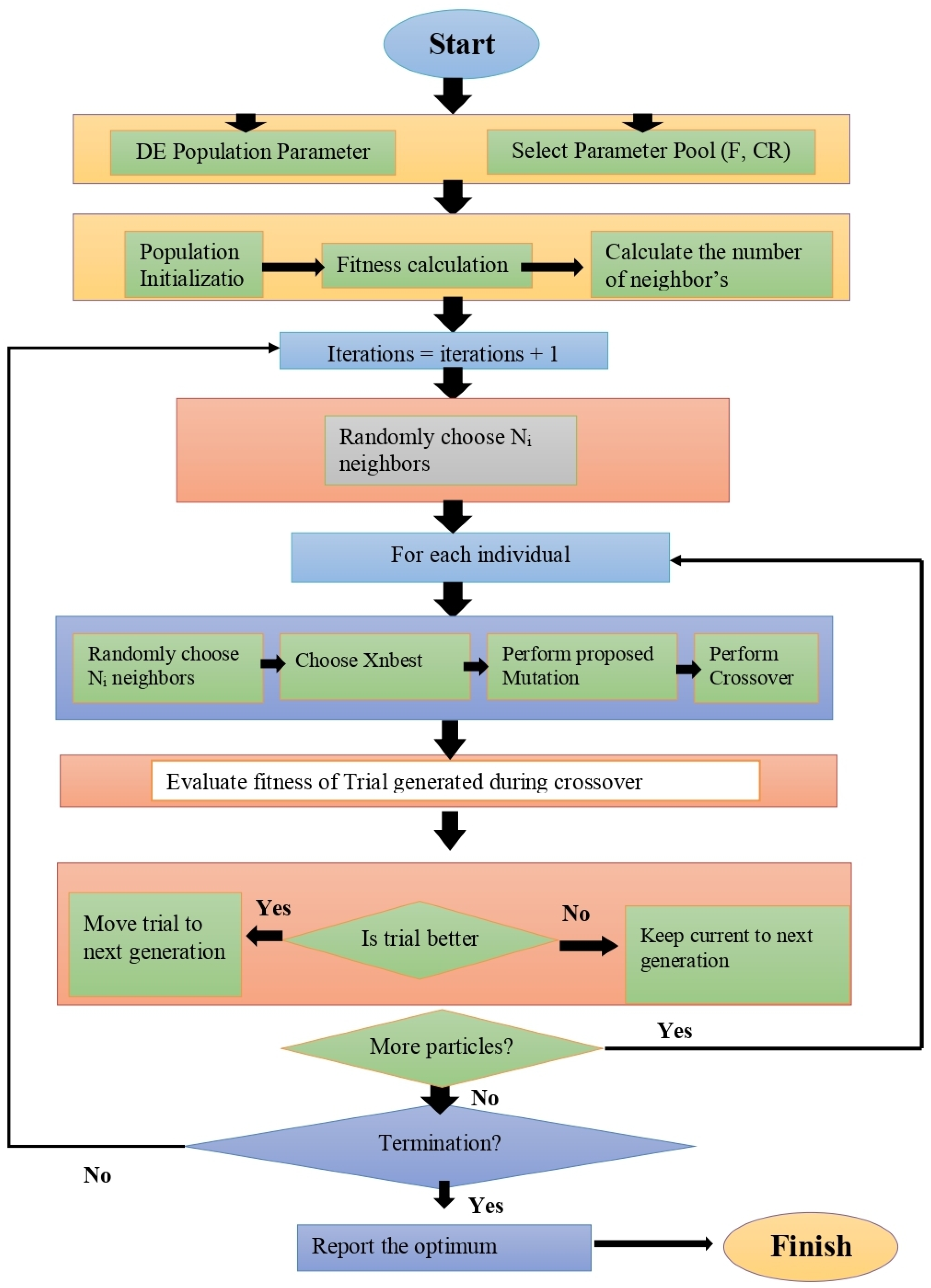
4.2. Proposed Approach
5. Results and Discussions
5.1. Parameter Settings
5.2. Benchmark Functions
5.3. Results
5.4. Statistical Significance
6. Conclusions
Author Contributions
Funding
Data Availability Statement
Acknowledgments
Conflicts of Interest
References
- Storn, R.; Price, K. Differential evolution–A simple and efficient heuristic for global optimization over continuous spaces. J. Glob. Optim. 1997, 11, 341–359. [Google Scholar] [CrossRef]
- Peng, H.; Guo, Z.; Deng, C.; Wu, Z. Enhancing differential evolution with random neighbors based strategy. J. Comput. Sci. 2018, 26, 501–511. [Google Scholar] [CrossRef]
- Deng, W.; Shang, S.; Cai, X.; Zhao, H.; Song, Y.; Xu, J. An improved differential evolution algorithm and its application in optimization problem. Soft Comput. 2021, 25, 5277–5298. [Google Scholar] [CrossRef]
- Hu, Z.; Gong, W.; Li, S. Reinforcement learning-based differential evolution for parameters extraction of photovoltaic models. Energy Rep. 2021, 7, 916–928. [Google Scholar] [CrossRef]
- Kharchouf, Y.; Herbazi, R.; Chahboun, A. Parameter’s extraction of solar photovoltaic models using an improved differential evolution algorithm. Energy Convers. Manag. 2022, 251, 114972. [Google Scholar] [CrossRef]
- Yu, X.; Liu, Z.; Wu, X.; Wang, X. A hybrid differential evolution and simulated annealing algorithm for global optimization. J. Intell. Fuzzy Syst. 2021, 41, 1375–1391. [Google Scholar] [CrossRef]
- Cheng, J.; Pan, Z.; Liang, H.; Gao, Z.; Gao, J. Differential evolution algorithm with fitness and diversity ranking-based mutation operator. Swarm Evol. Comput. 2021, 61, 100816. [Google Scholar] [CrossRef]
- Kumar, R.; Singh, K. A survey on soft computing-based high-utility itemsets mining. Soft Comput. 2022, 26, 1–46. [Google Scholar] [CrossRef]
- Abbas, Q.; Ahmad, J.; Jabeen, H. The analysis, identification and measures to remove inconsistencies from differential evolution mutation variants. Scienceasia 2017, 43S, 52–68. [Google Scholar] [CrossRef]
- Abbas, Q.; Ahmad, J.; Jabeen, H. A novel tournament selection based differential evolution variant for continuous optimization problems. Math. Probl. Eng. 2015, 2015, 1–21. [Google Scholar] [CrossRef]
- Li, J.; Yang, L.; Yi, J.; Yang, H.; Todo, Y.; Gao, S. A simple but efficient ranking-based differential evolution. IEICE Trans. Inf. Syst. 2022, 105, 189–192. [Google Scholar] [CrossRef]
- Kaliappan, P.; Ilangovan, A.; Muthusamy, S.; Sembanan, B. Temperature Control Design with Differential Evolution Based Improved Adaptive-Fuzzy-PID Techniques. Intell. Autom. Soft Comput. 2023, 36, 781–801. [Google Scholar] [CrossRef]
- Chen, X.; Shen, A. Self-adaptive differential evolution with Gaussian–Cauchy mutation for large-scale CHP economic dispatch problem. Neural Comput. Appl. 2022, 34, 11769–11787. [Google Scholar] [CrossRef]
- Deng, W.; Ni, H.; Liu, Y.; Chen, H.; Zhao, H. An adaptive differential evolution algorithm based on belief space and generalized opposition-based learning for resource allocation. Appl. Soft Comput. 2022, 127, 109419. [Google Scholar] [CrossRef]
- Abbas, Q.; Ahmad, J.; Jabeen, H. Random controlled pool base differential evolution algorithm (RCPDE). Intell. Autom. Soft Comput. 2017, 24, 377–390. [Google Scholar] [CrossRef]
- Thakur, S.; Dharavath, R.; Shankar, A.; Singh, P.; Diwakar, M.; Khosravi, M.R. RST-DE: Rough Sets-Based New Differential Evolution Algorithm for Scalable Big Data Feature Selection in Distributed Computing Platforms. Big Data 2022, 10, 356–367. [Google Scholar] [CrossRef]
- Zhan, Z.H.; Li, J.Y.; Zhang, J. Evolutionary deep learning: A survey. Neurocomputing 2022, 483, 42–58. [Google Scholar] [CrossRef]
- Awad, N.H.; Ali, M.Z.; Suganthan, P.N.; Reynolds, R.G. CADE: A hybridization of cultural algorithm and differential evolution for numerical optimization. Inf. Sci. 2017, 378, 215–241. [Google Scholar] [CrossRef]
- Fu, C.; Jiang, C.; Chen, G.; Liu, Q. An adaptive differential evolution algorithm with an aging leader and challengers mechanism. Appl. Soft Comput. 2017, 57, 60–73. [Google Scholar] [CrossRef]
- Awad, N.H.; Ali, M.Z.; Suganthan, P.N.; Jaser, E. A decremental stochastic fractal differential evolution for global numerical optimization. Inform. Sci. 2016, 372, 470–491. [Google Scholar] [CrossRef]
- Tian, M.; Gao, X.; Dai, C. Differential evolution with improved individual-based parameter setting and selection strategy. Appl. Soft Comput. 2017, 56, 286–297. [Google Scholar] [CrossRef]
- Zheng, L.M.; Zhang, S.X.; Tang, K.S.; Zheng, S.Y. Differential evolution powered by collective information. Inf. Sci. 2017, 399, 13–29. [Google Scholar] [CrossRef]
- Meng, Z.; Pan, J.S. QUasi-Affine TRansformation Evolution with External ARchive (QUATRE-EAR): An enhanced structure for differential evolution. Knowl.-Based Syst. 2018, 155, 35–53. [Google Scholar] [CrossRef]
- Sallam, K.M.; Elsayed, S.M.; Sarker, R.A.; Essam, D.L. Landscape-based adaptive operator selection mechanism for differential evolution. Inf. Sci. 2017, 418, 383–404. [Google Scholar] [CrossRef]
- Wu, G.; Shen, X.; Li, H.; Chen, H.; Lin, A.; Suganthan, P.N. Ensemble of differential evolution variants. Inf. Sci. 2018, 423, 172–186. [Google Scholar] [CrossRef]
- Cai, Y.; Liao, J.; Wang, T.; Chen, Y.; Tian, H. Social learning differential evolution. Inf. Sci. 2018, 433, 464–509. [Google Scholar] [CrossRef]
- Cai, Y.; Sun, G.; Wang, T.; Tian, H.; Chen, Y.; Wang, J. Neighborhood-adaptive differential evolution for global numerical optimization. Appl. Soft Comput. 2017, 59, 659–706. [Google Scholar] [CrossRef]
- Xiong, S.; Gong, W.; Wang, K. An adaptive neighborhood-based speciation differential evolution for multimodal optimization. Expert Syst. Appl. 2023, 211, 118571. [Google Scholar] [CrossRef]
- Liao, Z.; Zhu, F.; Mi, X.; Sun, Y. A neighborhood information-based adaptive differential evolution for solving complex nonlinear equation system model. Expert Syst. Appl. 2023, 216, 119455. [Google Scholar] [CrossRef]
- Gao, T.; Li, H.; Gong, M.; Zhang, M.; Qiao, W. Superpixel-based multiobjective change detection based on self-adaptive neighborhood-based binary differential evolution. Expert Syst. Appl. 2023, 212, 118811. [Google Scholar] [CrossRef]
- Liao, Z.; Mi, X.; Pang, Q.; Sun, Y. History archive assisted niching differential evolution with variable neighborhood for multimodal optimization. Swarm Evol. Comput. 2023, 76, 101206. [Google Scholar] [CrossRef]
- Liu, D.; Hu, Z.; Su, Q. Neighborhood-based differential evolution algorithm with direction induced strategy for the large-scale combined heat and power economic dispatch problem. Inf. Sci. 2022, 613, 469–493. [Google Scholar] [CrossRef]
- Sheng, M.; Chen, S.; Liu, W.; Mao, J.; Liu, X. A differential evolution with adaptive neighborhood mutation and local search for multi-modal optimization. Neurocomputing 2022, 489, 309–322. [Google Scholar] [CrossRef]
- Wang, Z.; Chen, Z.; Wang, Z.; Wei, J.; Chen, X.; Li, Q.; Zheng, Y.; Sheng, W. Adaptive memetic differential evolution with multi-niche sampling and neighborhood crossover strategies for global optimization. Inf. Sci. 2022, 583, 121–136. [Google Scholar] [CrossRef]
- Cai, Y.; Wu, D.; Zhou, Y.; Fu, S.; Tian, H.; Du, Y. Self-organizing neighborhood-based differential evolution for global optimization. Swarm Evol. Comput. 2020, 56, 100699. [Google Scholar] [CrossRef]
- Segredo, E.; Lalla-Ruiz, E.; Hart, E.; Voß, S. A similarity-based neighbourhood search for enhancing the balance exploration–Exploitation of differential evolution. Comput. Oper. Res. 2020, 117, 104871. [Google Scholar] [CrossRef]
- Baioletti, M.; Milani, A.; Santucci, V. Variable neighborhood algebraic differential evolution: An application to the linear ordering problem with cumulative costs. Inf. Sci. 2020, 507, 37–52. [Google Scholar] [CrossRef]
- Tian, M.; Gao, X. Differential evolution with neighborhood-based adaptive evolution mechanism for numerical optimization. Inf. Sci. 2019, 478, 422–448. [Google Scholar] [CrossRef]
- Tarkhaneh, O.; Moser, I. An improved differential evolution algorithm using Archimedean spiral and neighborhood search based mutation approach for cluster analysis. Future Gener. Comput. Syst. 2019, 101, 921–939. [Google Scholar] [CrossRef]


| Function | Name | Search Range | Global Optimum |
|---|---|---|---|
| Unimodal Functions | |||
| f1 | Sphere | [−100, 100] | 0 |
| f2 | Schwefel2.22 | [−10, 10] | 0 |
| f3 | Schwefel1.2 | [−100, 100] | 0 |
| f4 | Schwefel2.21 | [−100, 100] | 0 |
| f5 | Rosenbrock’s | [−30, 30] | 0 |
| f6 | Step | [−1.28, 1.28] | 0 |
| f7 | Quartic with Noise | [−100, 100] | 0 |
| Multimodal Functions | |||
| f8 | Schwefel2.26 | [−500, 500] | −418.98 |
| f9 | Rastrigin’s | [−5.12, 5.12] | 0 |
| f10 | Ackley | [−32, 32] | 0 |
| f11 | Griewank’s | [−600, 600] | 0 |
| f12 | Penalized1 | [−50, 50] | 0 |
| f13 | Penalized2 | [−50, 50] | 0 |
| Shifted Unimodal Functions | |||
| f14 | Shifted Sphere Function | [−100, 100] | −450 |
| f15 | Shifted Schwefel’s Problem 1.2 | [−100, 100] | −450 |
| f16 | Shifted Rotated High Conditioned Elliptic Function | [−100, 100] | −450 |
| f17 | Shifted Schwefel’s Problem 1.2 with Noise in Fitness | [−100, 100] | −450 |
| f18 | Schwefel’s Problem 2.6 with Global Optimum on Bounds | [−100, 100] | −310 |
| Shifted Multimodal Functions | |||
| f19 | Shifted Rosenbrock’s Function | [−100, 100] | 390 |
| f20 | Shifted Rotated Griewank’s Function without Bounds | [0, 600] | −180 |
| f21 | Shifted Rotated Ackley’s Function with Global Optimum on Bounds | [−32, 32] | −140 |
| f22 | Shifted Rastrigin’s Function | [−5, 5] | −330 |
| f23 | Shifted Rotated Rastrigin’s Function | [−5, 5] | −330 |
| f24 | Shifted Rotated Weierstrass Function | [−0.5, 0.5] | 90 |
| f25 | Schwefel’s Problem 2.13 | [, ] | −460 |
| f26 | Shifted Expanded Griewank’s plus Rosenbrock’s Function (F8F2) | [−3, 1] | −130 |
| f27 | Shifted Rotated Expanded Scaffer’s F6 Function | [−100, 100] | −300 |
| Iterations | f1 | f2 | f3 | f4 | f5 | |||||
|---|---|---|---|---|---|---|---|---|---|---|
| RNDE | IRNDE | RNDE | IRNDE | RNDE | IRNDE | RNDE | IRNDE | RNDE | IRNDE | |
| 1 | 107,166 | 107,166 | 197,013 | 197,013 | 91.4529 | 91.4529 | 2.19833e+71 | 2.19833e+71 | 4.31944e+08 | 4.31944e+08 |
| 5 | 107,166 | 107,166 | 197,013 | 197,013 | 91.4529 | 91.4529 | 1.56318e+71 | 1.25631e+69 | 4.31944e+08 | 4.31944e+08 |
| 10 | 106,763 | 98,577.1 | 197,013 | 197,013 | 91.4529 | 91.4529 | 1.56318e+71 | 9.13478e+68 | 4.31944e+08 | 4.31944e+08 |
| 15 | 106,763 | 98577.1 | 197,013 | 197,013 | 91.4529 | 91.4529 | 1.36815e+71 | 6.45164e+68 | 4.31944e+08 | 4.31944e+08 |
| 20 | 106,763 | 98577.1 | 196,295 | 168,441 | 91.4529 | 91.4529 | 6.09134e+69 | 5.62354e+67 | 4.31944e+08 | 4.31944e+08 |
| 30 | 102,924 | 93,241.7 | 196,295 | 168,441 | 91.4529 | 91.4529 | 1.10354e+69 | 3.20042e+67 | 4.31944e+08 | 4.31944e+08 |
| 40 | 93,490.6 | 93,241.7 | 196,295 | 168,441 | 91.4529 | 91.4529 | 8.49963e+68 | 1.1789e+65 | 4.31944e+08 | 4.31944e+08 |
| 50 | 93,490.6 | 91,660.3 | 196,295 | 168,441 | 91.4529 | 91.4529 | 3.2853e+67 | 6.41441e+63 | 4.31944e+08 | 4.31944e+08 |
| 100 | 86,431.9 | 56,403.3 | 196,295 | 168,441 | 91.4065 | 89.2837 | 1.27491e+63 | 3.44804e+55 | 4.04911e+08 | 2.99116e+08 |
| 150 | 69,868.9 | 40,416.5 | 171,358 | 143,138 | 90.3058 | 89.2837 | 1.15333e+62 | 5.90041e+53 | 4.04911e+08 | 2.77088e+08 |
| 200 | 64,281 | 34,341.9 | 171,358 | 143,138 | 90.3058 | 89.0754 | 4.09299e+60 | 2.93405e+51 | 3.90937e+08 | 1.99466e+08 |
| 400 | 31,954.4 | 6800.34 | 164,102 | 113,800 | 89.5071 | 85.3248 | 8.52268e+57 | 6.13965e+47 | 2.92851e+08 | 1.51033e+07 |
| 600 | 17,025.5 | 1761.99 | 153,406 | 96,057.6 | 89.5071 | 74.6393 | 5.21376e+49 | 9.92589e+44 | 2.45835e+08 | 1.92694e+06 |
| 800 | 7159.23 | 271.509 | 153,406 | 96,057.6 | 88.0884 | 67.8502 | 1.49244e+47 | 4.0476e+43 | 1.54781e+08 | 350747 |
| 1000 | 2954.65 | 85.033 | 113,349 | 78,643.5 | 85.2505 | 56.0395 | 2.36147e+46 | 3.02577e+42 | 5.83435e+07 | 57207.6 |
| 1200 | 1411.61 | 12.6946 | 113,349 | 78571.1 | 81.3025 | 51.9173 | 4.34581e+45 | 7.79156e+40 | 1.66845e+07 | 23060.8 |
| 1400 | 705.528 | 3.36049 | 113,349 | 78,508.4 | 64.4952 | 43.103 | 3.27444e+42 | 1.04872e+38 | 1.06145e+07 | 6365.95 |
| 1600 | 330.4 | 0.705804 | 103,116 | 77,692 | 64.4952 | 38.9589 | 2.92916e+37 | 9.65888e+34 | 3.61785e+06 | 3784.11 |
| 1800 | 143.321 | 0.148906 | 103,116 | 76,766.7 | 58.7125 | 27.6752 | 2.68602e+33 | 1.27846e+34 | 1.06625e+06 | 1897.68 |
| 2000 | 72.6645 | 0.027825 | 102008 | 70697.2 | 49.5419 | 24.4122 | 2.62547e+33 | 1.74314e+32 | 861487 | 1077.72 |
| 2200 | 28.5524 | 0.00816997 | 100,863 | 61497.6 | 48.856 | 21.7797 | 2.3213e+31 | 2.27938e+30 | 263,768 | 916.068 |
| 2400 | 15.1582 | 0.00170155 | 97,335.3 | 51,589.8 | 43.1867 | 18.7337 | 2.27744e+30 | 1.26613e+27 | 195775 | 700.118 |
| 2600 | 5.75624 | 0.000385194 | 94,308.2 | 51,589.8 | 39.6438 | 14.7789 | 2.27744e+30 | 2.4849e+26 | 112,458 | 642.347 |
| 2800 | 2.84793 | 8.46806e-05 | 94308.2 | 46713.4 | 36.3745 | 12.6463 | 1.06585e+30 | 1.44058e+26 | 108,988 | 578.795 |
| 3000 | 1.30338 | 1.73096e-05 | 89,843.4 | 45,302.9 | 32.3394 | 9.99071 | 3.97908e+28 | 2.10136e+24 | 80144.5 | 515.251 |
| 3200 | 0.591442 | 4.38451e-06 | 89,843.4 | 38085.9 | 27.8329 | 8.72914 | 3.97908e+28 | 9.46517e+23 | 49,036 | 462.433 |
| 3400 | 0.243082 | 1.02105e-06 | 85,722.3 | 38,085.9 | 25.2841 | 6.37169 | 3.97908e+28 | 2.44522e+22 | 38,846.7 | 347.158 |
| 3600 | 0.112868 | 2.96409e-07 | 58,333.6 | 37,141.8 | 25.2841 | 0.4367 | 3.97908e+28 | 3.53667e+20 | 30,109.7 | 347.158 |
| 3800 | 0.0454132 | 4.85207e-08 | 58,087.2 | 33,533.5 | 22.1458 | 4.33106 | 3.97908e+28 | 3.23352e+19 | 21,079.1 | 301.099 |
| 4000 | 0.0233552 | 1.12556e-08 | 58,087.2 | 32429.3 | 20.2136 | 3.77252 | 1.09389e+28 | 1.09388e+18 | 19,657.9 | 248.39 |
| 4200 | 0.0104778 | 2.35218e-09 | 50,409.5 | 28,602.2 | 19.4409 | 3.06997 | 2.02774e+26 | 5.27283e+16 | 13542.1 | 188.169 |
| 4400 | 0.00507579 | 3.57897e-10 | 48,908.5 | 24,143 | 16.6239 | 2.6146 | 1.14581e+21 | 2.90392e+16 | 7989.71 | 129.291 |
| 4600 | 0.00191955 | 5.69887e-11 | 48,908.5 | 21,842.5 | 14.7613 | 2.18745 | 1.14581e+21 | 4.48367e+12 | 5393.15 | 75.9085 |
| 4800 | 0.000790519 | 1.34205e-11 | 48,908.5 | 19,772.3 | 14.4084 | 1.63888 | 1.14581e+21 | 1.43737e+11 | 4743.71 | 56.1816 |
| 5000 | 0.000285069 | 2.70302e-12 | 48,861.7 | 19,772.3 | 12.7042 | 1.38764 | 1.14581e+21 | 1.43737e+11 | 4269.41 | 49.7603 |
| Iterations | f6 | f7 | f8 | f9 | f10 | |||||
|---|---|---|---|---|---|---|---|---|---|---|
| RNDE | IRNDE | RNDE | IRNDE | RNDE | IRNDE | RNDE | IRNDE | RNDE | IRNDE | |
| 1 | 21 | 21 | 1.42628e+10 | 1.42628e+10 | −3516.54 | −3516.54 | 728.486 | 728.486 | 20.7073 | 20.7073 |
| 5 | 20 | 21 | 1.42628e+10 | 1.42628e+10 | −4303.27 | −4484.28 | 710.839 | 728.486 | 20.7073 | 20.7073 |
| 10 | 20 | 19 | 1.42628e+10 | 1.42628e+10 | −6262.3 | −6764.29 | 710.839 | 728.486 | 20.6636 | 20.6009 |
| 15 | 20 | 19 | 1.42628e+10 | 1.42628e+10 | −6282.13 | −6935.1 | 710.839 | 724.258 | 20.6636 | 20.6009 |
| 20 | 20 | 19 | 1.42628e+10 | 1.12205e+10 | −7428.17 | −10,057 | 710.839 | 724.258 | 20.6636 | 20.5467 |
| 30 | 20 | 16 | 1.42628e+10 | 1.12205e+10 | −9398.02 | −14,537.2 | 710.839 | 724.258 | 20.6381 | 20.5467 |
| 40 | 20 | 16 | 1.42628e+10 | 1.05978e+10 | −9534.25 | −16,106.3 | 710.839 | 682.222 | 20.5408 | 20.5467 |
| 50 | 20 | 16 | 1.32638e+10 | 1.05978e+10 | −10322.7 | −19,528.8 | 710.839 | 679.314 | 20.4485 | 20.4571 |
| 100 | 17 | 13 | 1.26344e+10 | 6.24556e+09 | −12489.3 | −20,949 | 698.499 | 594.514 | 20.3311 | 19.7722 |
| 150 | 16 | 11 | 1.17699e+10 | 3.04017e+09 | −14,918.2 | −20,949 | 698.499 | 533.429 | 19.8555 | 19.2148 |
| 200 | 15 | 7 | 1.17699e+10 | 1.56747e+09 | −16,420 | −20,949 | 698.499 | 494.476 | 19.7466 | 17.9631 |
| 400 | 10 | 2 | 5.23897e+09 | 2.18584e+08 | −20,949 | −20,949 | 698.499 | 455.163 | 18.7771 | 13.0003 |
| 600 | 7 | 0 | 4.14472e+09 | 1.98573e+07 | −20,949 | −20,949 | 698.499 | 404.723 | 16.8826 | 8.77267 |
| 800 | 4 | 0 | 1.17689e+09 | 2.39732e+06 | −20,949 | −20,949 | 698.499 | 362.02 | 14.5523 | 5.26086 |
| 1000 | 4 | 0 | 2.94735e+08 | 229054 | −20,949 | −20,949 | 682.614 | 362.02 | 12.3433 | 3.72313 |
| 1200 | 3 | 0 | 5.57891e+07 | 34096.6 | −20,949 | −20,949 | 682.614 | 352.496 | 9.90552 | 2.51792 |
| 1400 | 2 | 0 | 1.79379e+07 | 2328.99 | −20,949 | −20,949 | 682.614 | 349.761 | 7.68546 | 1.84401 |
| 1600 | 2 | 0 | 4.92482e+06 | 268.371 | −20,949 | −20,949 | 682.614 | 349.212 | 5.72134 | 0.697559 |
| 1800 | 1 | 0 | 1.60315e+06 | 22.3301 | −20,949 | −20,949 | 661.983 | 349.212 | 4.52571 | 0.242736 |
| 2000 | 1 | 0 | 291,084 | 1.7914 | −20,949 | −20,949 | 661.983 | 349.212 | 4.08072 | 0.0935032 |
| 2200 | 1 | 0 | 149,086 | 0 | −20,949 | −20,949 | 661.983 | 346.007 | 3.42992 | 0.0420455 |
| 2400 | 1 | 0 | 64,393.3 | 0 | −20,949 | −20,949 | 661.983 | 346.007 | 2.92868 | 0.01849 |
| 2600 | 0 | 0 | 22,563.6 | 0 | −20,949 | −20,949 | 661.983 | 346.007 | 2.76194 | 0.00828884 |
| 2800 | 0 | 0 | 6538.42 | 0 | −20,949 | −20,949 | 661.983 | 346.007 | 2.45848 | 0.00367194 |
| 3000 | 0 | 0 | 1510.69 | 0 | −20,949 | −20,949 | 645.042 | 323.189 | 2.18228 | 0.00170531 |
| 3200 | 0 | 0 | 434.261 | 0 | −20,949 | −20,949 | 645.042 | 323.189 | 1.65711 | 0.00071923 |
| 3400 | 0 | 0 | 96.3754 | 0 | −20,949 | −20,949 | 637.334 | 323.189 | 0.958296 | 0.000306232 |
| 3600 | 0 | 0 | 29.8399 | 0 | −20,949 | −20,949 | 637.334 | 319.548 | 0.389258 | 0.000158771 |
| 3800 | 0 | 0 | 6.60063 | 0 | −20,949 | −20,949 | 618.245 | 319.548 | 0.233483 | 6.64578e-05 |
| 4000 | 0 | 0 | 3.47587 | 0 | −20,949 | −20,949 | 618.245 | 319.548 | 0.176824 | 3.53399e-05 |
| 4200 | 0 | 0 | 0 | 0 | −20,949 | −20,949 | 618.245 | 311.84 | 0.113753 | 1.68176e-05 |
| 4400 | 0 | 0 | 0 | 0 | −20,949 | −20,949 | 618.245 | 311.84 | 0.0665963 | 6.99799e-06 |
| 4600 | 0 | 0 | 0 | 0 | −20,949 | −20,949 | 618.245 | 311.84 | 0.041563 | 3.74626e-06 |
| 4800 | 0 | 0 | 0 | 0 | −20,949 | −20,949 | 601.333 | 311.84 | 0.0263947 | 1.71841e-06 |
| 5000 | 0 | 0 | 0 | 0 | −20,949 | −20,949 | 601.333 | 311.84 | 0.0188713 | 8.13691e-07 |
| Iterations | f11 | f12 | f13 | f14 | f15 | |||||
|---|---|---|---|---|---|---|---|---|---|---|
| RNDE | IRNDE | RNDE | IRNDE | RNDE | IRNDE | RNDE | IRNDE | RNDE | IRNDE | |
| 1 | 1055.15 | 1055.15 | 1.08539e+09 | 1.08539e+09 | 2.00701e+09 | 2.00701e+09 | 168,301 | 168,301 | 398,585 | 398,585 |
| 5 | 1055.15 | 1055.15 | 1.0548e+09 | 1.08539e+09 | 2.00701e+09 | 2.00701e+09 | 159,042 | 166,735 | 355,510 | 334,098 |
| 10 | 1055.15 | 1039.8 | 1.05323e+09 | 1.08539e+09 | 2.00701e+09 | 2.00701e+09 | 125,808 | 163,621 | 355,510 | 283,650 |
| 15 | 1055.15 | 1039.8 | 1.05323e+09 | 1.08539e+09 | 2.00701e+09 | 2.00701e+09 | 125,808 | 162,531 | 335,683 | 250,962 |
| 20 | 1052.27 | 937.941 | 1.05323e+09 | 1.08539e+09 | 2.00701e+09 | 2.00701e+09 | 120,207 | 131,129 | 335,683 | 250,962 |
| 30 | 1052.27 | 937.941 | 1.05323e+09 | 1.08539e+09 | 2.00701e+09 | 2.00701e+09 | 120,207 | 118,288 | 335,683 | 250,962 |
| 40 | 1052.27 | 894.572 | 1.05323e+09 | 1.08539e+09 | 2.00701e+09 | 2.00701e+09 | 106,490 | 114,755 | 335,683 | 250,962 |
| 50 | 1002.21 | 710.905 | 1.05323e+09 | 1.08539e+09 | 2.00701e+09 | 2.00701e+09 | 106,490 | 109,345 | 263,847 | 228,577 |
| 100 | 1002.21 | 542.417 | 1.05323e+09 | 1.01396e+09 | 1.88035e+09 | 1.94988e+09 | 85847.8 | 64180.9 | 224,621 | 185,333 |
| 150 | 1002.21 | 347.765 | 1.05323e+09 | 5.11633e+08 | 1.88035e+09 | 1.11306e+09 | 81634.2 | 55196.3 | 224,621 | 155,871 |
| 200 | 966.712 | 270.401 | 9.49775e+08 | 4.21792e+08 | 1.84609e+09 | 8.48217e+08 | 69772.1 | 34856.8 | 224,452 | 155,871 |
| 400 | 917.708 | 52.6602 | 5.81916e+08 | 3.97822e+07 | 1.3873e+09 | 7.41636e+07 | 24635.1 | 5930.8 | 209,400 | 152,495 |
| 600 | 917.708 | 13.7598 | 5.63661e+08 | 953763 | 1.26871e+09 | 3.5074e+06 | 12060.9 | 1400.9 | 177,338 | 144,816 |
| 800 | 759.071 | 3.21318 | 4.32972e+08 | 1005.07 | 1.2686e+09 | 43217.1 | 5247.32 | −48.6701 | 170,882 | 125,566 |
| 1000 | 729.991 | 1.60481 | 2.97419e+08 | 22.796 | 7.18698e+08 | 767.809 | 2420.72 | −370.845 | 154,607 | 97,994.6 |
| 1200 | 632.36 | 1.10341 | 4.74073e+07 | 9.4321 | 4.88062e+08 | 38.0572 | 838.294 | −432.312 | 154,607 | 97,768.6 |
| 1400 | 564.399 | 1.01736 | 1.54405e+07 | 4.53885 | 1.71841e+08 | 16.5448 | 114.425 | −446.984 | 153,222 | 94,129.1 |
| 1600 | 450.362 | 0.658333 | 3.30737e+06 | 4.25549 | 4.75411e+07 | 3.86112 | −167.851 | −449.317 | 153,222 | 79,506.3 |
| 1800 | 272.759 | 0.22698 | 310,283 | 2.83376 | 1.47191e+07 | 1.10332 | -296.65 | −449.78 | 141,583 | 77,475.6 |
| 2000 | 254.433 | 0.0445405 | 75,962.6 | 2.3151 | 3.43088e+06 | 0.308245 | −398.253 | −449.961 | 135,500 | 74,589.6 |
| 2200 | 198.676 | 0.00737067 | 126.916 | 2.12297 | 1.16831e+06 | 0.0776809 | −424.14 | −449.993 | 135,500 | 69,304.9 |
| 2400 | 124.491 | 0.00171678 | 31.6576 | 1.76203 | 258,691 | 0.0147251 | −437.264 | −449.998 | 127,620 | 62,349.5 |
| 2600 | 96.0986 | 0.000409527 | 19.7927 | 1.47519 | 19,247.4 | 0.00279349 | −444.947 | −450 | 127,620 | 56,522 |
| 2800 | 66.9394 | 9.89848e-05 | 12.1895 | 0.995179 | 296.106 | 0.000594427 | −446.741 | −450 | 123,796 | 55,272.9 |
| 3000 | 46.4022 | 2.55152e-05 | 11.0036 | 0.913088 | 62.8248 | 0.000129401 | −449.27 | −450 | 121,615 | 51,567.8 |
| 3200 | 34.6919 | 5.18012e-06 | 7.55257 | 0.536102 | 52.5342 | 2.94385e-05 | −449.568 | −450 | 112,014 | 47,125.5 |
| 3400 | 21.599 | 6.62209e-07 | 6.5113 | 0.282837 | 33.2308 | 7.30486e-06 | −449.82 | −450 | 97,448.5 | 45,670.9 |
| 3600 | 17.9387 | 1.96707e-07 | 6.23303 | 0.0455196 | 14.0115 | 1.12448e-06 | −449.929 | −450 | 97,356.9 | 44,078.9 |
| 3800 | 10.8625 | 4.72381e-08 | 5.51551 | 0.00797489 | 6.56287 | 2.64319e-07 | −449.976 | −450 * | 95,037.9 | 43,505.3 |
| 4000 | 7.99392 | 9.67328e-09 | 3.45958 | 0.00158262 | 3.8305 | 5.15215e-08 | −449.988 | −450 | 95,037.9 | 30,530.6 |
| 4200 | 5.55138 | 1.67994e-09 | 3.33907 | 0.000302378 | 1.87559 | 6.99077e-09 | −449.994 | −450 | 79,005.2 | 28,242.5 |
| 4400 | 4.71148 | 4.01571e-10 | 3.33907 | 6.66714e-05 | 0.657885 | 1.60463e-09 | −449.997 | −450 | 79,005.2 | 27,167.2 |
| 4600 | 3.69465 | 6.71285e-11 | 3.27146 | 1.49248e-05 | 0.458076 | 2.50137e-10 | −449.999 | −450 | 79,005.2 | 27,167.2 |
| 4800 | 2.52784 | 1.32597e-11 | 3.27146 | 3.3658e-06 | 0.255931 | 5.15735e-11 | −450 | −450 | 76,609.3 | 18,035 |
| 5000 | 2.1493 | 2.38842e-12 | 3.27146 | 6.39102e-07 | 0.107353 | 9.56412e-12 | −450* | −450 | 69,629.2 | 17,402.5 |
| 10 Runs Fitness Evaluations for NP = 150/D = 10 | |||||||
|---|---|---|---|---|---|---|---|
| Best | Median | Worst | Mean ± Std. Dev. | Success Rate | RNDE vs. IRNDE (# of Iterations) | ||
| f1 | RNDE | 504 | 518 | 526 | 5.157e+2 ± 8.68012e+0 | 100% | 516 |
| IRNDE | 340 | 345 | 357 | 3.468e+2 ± 5.05085e+0 | 100% | 348 | |
| f2 | RNDE | 1457 | 1480 | 1528 | 1.4885e+3 ± 2.25549e+1 | 100% | 1549 |
| IRNDE | 784 | 819 | 875 | 8.26e+2 ± 3.32031e+1 | 100% | 802 | |
| f3 | RNDE | 820 | 846 | 874 | 8.456e+2 ± 1.42533e+1 | 100% | 477 |
| IRNDE | 590 | 625 | 647 | 6.207e+2 ± 1.82638e+1 | 100% | 336 | |
| f4 | RNDE | 808 | 823 | 847 | 8.251e+2 ± 1.19856e+1 | 100% | 832 |
| IRNDE | 342 | 349 | 359 | 3.495e+2 ± 5.01664e+0 | 100% | 618 | |
| f5 | RNDE | 1652 | 1715 | 1757 | 1.7163e+3 ± 3.54622e+1 | 100% | 1737 |
| IRNDE | 1034 | 1072 | 1132 | 1.0773e+3 ± 3.23661e+1 | 100% | 1087 | |
| f6 | RNDE | 1 | 15 | 27 | 1.45e+1 ± 7.15309e+0 | 100% | 13 |
| IRNDE | 7 | 13 | 22 | 1.34e+1 ± 4.29987e+0 | 100% | 12 | |
| f7 | RNDE | 187 | 192 | 204 | 1.955e+2 ± 6.62067e+0 | 100% | 205 |
| IRNDE | 122 | 132 | 139 | 1.316e+2 ± 5.05964e+0 | 100% | 138 | |
| f8 | RNDE | 18 | 27 | 31 | 2.66e+1 ± 3.62706e+0 | 100% | 30 |
| IRNDE | 9 | 11 | 17 | 1.22e+1 ± 2.65832e+0 | 100% | 11 | |
| f9 | RNDE | 830 | 871 | 908 | 8.742e+2 ± 2.23696e+1 | 100% | 915 |
| IRNDE | 906 | 1126 | 1265 | 1.1178e+3 ± 1.04919e+2 | 100% | 1227 | |
| f10 | RNDE | 797 | 817 | 839 | 8.198e+2 ± 1.18771e+1 | 100% | 815 |
| IRNDE | 552 | 565 | 574 | 5.653e+2 ± 7.33409e+0 | 100% | 569 | |
| f11 | RNDE | 1729 | 2065 | 2328 | 2.037e+3 ± 2.02333e+2 | 100% | 2621 |
| IRNDE | 1996 | 2586 | 3700 | 2.7613e+3 ± 5.16669e+2 | 100% | 3453 | |
| f12 | RNDE | 446 | 468 | 493 | 4.671e+2 ± 1.26179e+1 | 100% | 484 |
| IRNDE | 321 | 331 | 344 | 3.327e+2 ± 7.39444e+0 | 100% | 328 | |
| f13 | RNDE | 472 | 488 | 506 | 4.879e+2 ± 1.13671e+1 | 100% | 476 |
| IRNDE | 332 | 338 | 346 | 3.393e+2 ± 4.49815e+0 | 100% | 327 | |
| f14 | RNDE | 503 | 511 | 524 | 5.112e+2 ± 6.47731e+0 | 100% | 503 |
| IRNDE | 337 | 353 | 359 | 3.512e+2 ± 7.56894e+0 | 100% | 353 | |
| f15 | RNDE | 1440 | 1484 | 1558 | 1.4951e+3 ± 3.86018e+1 | 100% | 1539 |
| IRNDE | 810 | 824 | 887 | 8.363e+2 ± 2.70803e+1 | 100% | 858 | |
| f16 | RNDE | 496 | 522 | 542 | 5.204e+2 ± 1.26947e+1 | 100% | 499 |
| IRNDE | 343 | 350 | 359 | 3.519e+2 ± 5.95259e+0 | 100% | 345 | |
| f17 | RNDE | 1471 | 1532 | 1603 | 1.5474e+3 ± 4.45676e+1 | 100% | 1496 |
| IRNDE | 844 | 858 | 907 | 8.693e+2 ± 2.34902e+1 | 100% | 832 | |
| f18 | RNDE | 616 | 643 | 679 | 6.494e+2 ± 1.96932e+1 | 100% | 652 |
| IRNDE | 513 | 535 | 558 | 5.346e+2 ± 1.12862e+1 | 100% | 518 | |
| f19 | RNDE | 265 | 274 | 295 | 2.777e+2 ± 9.84378e+0 | 100% | 265 |
| IRNDE | 220 | 227 | 238 | 2.292e+2 ± 5.82714e+0 | 100% | 233 | |
| f20 | RNDE | 400 | 431 | 484 | 4.396e+2 ± 2.63236e+1 | 100% | 518 |
| IRNDE | 228 | 261 | 308 | 2.683e+2 ± 2.55345e+1 | 100% | 352 | |
| f21 | RNDE | 343 | 355 | 369 | 3.562e+2 ± 8.25698e+0 | 100% | 365 |
| IRNDE | 297 | 304 | 320 | 3.063e+2 ± 8.28721e+0 | 100% | 310 | |
| f22 | RNDE | 388 | 396 | 411 | 3.991e+2 ± 7.37036e+0 | 100% | 393 |
| IRNDE | 257 | 268 | 274 | 2.681e+2 ± 5.21643e+0 | 100% | 267 | |
| f23 | RNDE | 286 | 308 | 316 | 3.066e+2 ± 1.01784e+1 | 100% | 306 |
| IRNDE | 195 | 206 | 213 | 2.059e+2 ± 5.46606e+0 | 100% | 196 | |
| f24 | RNDE | 761 | 803 | 831 | 8.008e+2 ± 1.98203e+1 | 100% | 773 |
| IRNDE | 616 | 634 | 649 | 6.343e+2 ± 1.09143e+1 | 100% | 612 | |
| f25 | RNDE | 3620 | 5080 | 9495 | 5.83986e+3 ± 2.00043e+3 | 70% | 3217 |
| IRNDE | 286 | 423 | 1088 | 4.74111e+2 ± 2.39794e+2 | 90% | 1608 | |
| f26 | RNDE | 179 | 182 | 216 | 1.918e+2 ± 1.31976e+1 | 100% | 172 |
| IRNDE | 108 | 117 | 123 | 1.164e+2 ± 4.16867e+0 | 100% | 127 | |
| f27 | RNDE | 214 | 223 | 229 | 2.234e+2 ± 4.74224e+0 | 100% | 228 |
| IRNDE | 162 | 169 | 171 | 1.683e+2 ± 2.71006e+0 | 100% | 169 | |
| 10 Runs Fitness Evaluations for NP = 150/D = 30 | |||||||
|---|---|---|---|---|---|---|---|
| Best | Median | Worst | Mean ± Std. Dev. | Success Rate | RNDE vs. IRNDE (# of Iterations) | ||
| f1 | RNDE | 2555 | 2627 | 2745 | 2.6491e+3 ± 6.40424e+1 | 100% | 2675 |
| IRNDE | 1736 | 1753 | 1792 | 1.7634e+3 ± 2.09401e+1 | 100% | 1802 | |
| f2 | RNDE | 57,202 | 59,993 | 66,380 | 6.05669e+4 ± 2.46933e+3 | 100% | 57,718 |
| IRNDE | 23,162 | 23,828 | 24,961 | 2.39414e+4 ± 5.28169e+2 | 100% | 24,016 | |
| f3 | RNDE | 8581 | 8825 | 9258 | 8.9154e+3 ± 2.28402e+2 | 100% | 9119 |
| IRNDE | 5464 | 5532 | 5841 | 5.6021e+3 ± 1.32403e+2 | 100% | 5546 | |
| f4 | RNDE | 4294 | 4340 | 4476 | 4.356e+3 ± 6.34333e+1 | 100% | 4480 |
| IRNDE | 3086 | 3169 | 3395 | 3.1891e+3 ± 8.24155e+1 | 100% | 3303 | |
| f5 | RNDE | 12504 | 12915 | 13721 | 1.30622e+4 ± 4.15667e+2 | 100% | 13,426 |
| IRNDE | 7377 | 7580 | 7803 | 7.5919e+3 ± 1.51639e+2 | 100% | 7659 | |
| f6 | RNDE | 179 | 225 | 272 | 2.27e+2 ± 3.39706e+1 | 100% | 227 |
| IRNDE | 118 | 143 | 168 | 1.437e+2 ± 1.75439e+1 | 100% | 142 | |
| f7 | RNDE | 1150 | 1224 | 1289 | 1.2318e+3 ± 4.22816e+1 | 100% | 1239 |
| IRNDE | 811 | 840 | 902 | 8.455e+2 ± 2.53213e+1 | 100% | 886 | |
| f8 | RNDE | 70 | 108 | 137 | 1.017e+2 ± 2.17718e+1 | 100% | 102 |
| IRNDE | 25 | 35 | 58 | 3.68e+1 ± 8.9666e+0 | 100% | 52 | |
| f9 | RNDE | 39881 | 43,293 | 48,764 | 4.37697e+4 ± 2.6549e+3 | 100% | 41,835 |
| IRNDE | - | - | - | - | 0% | 6.58946e+1 | |
| f10 | RNDE | 3998 | 4089 | 4208 | 4.0932e+3 ± 7.4265e+1 | 100% | 4147 |
| IRNDE | 2700 | 2730 | 2770 | 2.7372e+3 ± 2.18469e+1 | 100% | 2718 | |
| f11 | RNDE | 4072 | 4147 | 4297 | 4.1676e+3 ± 8.43567e+1 | 100% | 4146 |
| IRNDE | 1827 | 2017 | 2161 | 2.0213e+3 ± 1.14815e+2 | 100% | 2092 | |
| f12 | RNDE | 2569 | 2701 | 2840 | 2.6904e+3 ± 7.63081e+1 | 100% | 2782 |
| IRNDE | 1719 | 1739 | 1823 | 1.7558e+3 ± 3.35354e+1 | 100% | 1752 | |
| f13 | RNDE | 2586 | 2616 | 2719 | 2.6462e+3 ± 5.21575e+1 | 100% | 2661 |
| IRNDE | 1738 | 1769 | 1838 | 1.7794e+3 ± 3.34139e+1 | 100% | 1809 | |
| f14 | RNDE | 2646 | 2667 | 2742 | 2.6824e+3 ± 3.43615e+1 | 100% | 2630 |
| IRNDE | 1746 | 1780 | 1833 | 1.7887e+3 ± 3.41989e+1 | 100% | 1867 | |
| f15 | RNDE | 58341 | 60,131 | 62,726 | 6.07395e+4 ± 1.69443e+3 | 100% | 59,989 |
| IRNDE | 23,938 | 24,436 | 24,956 | 2.44474e+4 ± 3.02649e+2 | 100% | 23,667 | |
| f16 | RNDE | 2574 | 2642 | 2752 | 2.651e+3 ± 5.04094e+1 | 100% | 2674 |
| IRNDE | 1770 | 1803 | 1842 | 1.8056e+3 ± 2.39499e+1 | 100% | 1780 | |
| f17 | RNDE | 61,575 | 61,985 | 65,619 | 6.29908e+4 ± 1.38551e+3 | 100% | 62,862 |
| IRNDE | 25,129 | 26,032 | 27,197 | 2.62584e+4 ± 7.24199e+2 | 100% | 27,668 | |
| f18 | RNDE | 4695 | 4781 | 4878 | 4.7949e+3 ± 6.23154e+1 | 100% | 4890 |
| IRNDE | 3486 | 3638 | 3821 | 3.6549e+3 ± 8.90661e+1 | 100% | 3741 | |
| f19 | RNDE | 1018 | 1039 | 1088 | 1.0458e+3 ± 1.88255e+1 | 100% | 1023 |
| IRNDE | 805 | 823 | 844 | 8.251e+2 ± 1.46246e+1 | 100% | 803 | |
| f20 | RNDE | 4386 | 4728 | 5203 | 4.7566e+3 ± 2.72762e+2 | 100% | 4829 |
| IRNDE | 2633 | 2936 | 3887 | 3.0857e+3 ± 3.68177e+2 | 100% | 3050 | |
| f21 | RNDE | 1257 | 1279 | 1311 | 1.2815e+3 ± 1.75768e+1 | 100% | 1307 |
| IRNDE | 1029 | 1050 | 1056 | 1.0457e+3 ± 1.02746e+1 | 100% | 1082 | |
| f22 | RNDE | 2078 | 2151 | 2228 | 2.1589e+3 ± 4.80681e+1 | 100% | 2653 |
| IRNDE | 1399 | 1424 | 1507 | 1.4387e+3 ± 3.33801e+1 | 100% | 1532 | |
| f23 | RNDE | 1629 | 1685 | 1734 | 1.6867e+3 ± 3.29209e+1 | 100% | 1699 |
| IRNDE | 1084 | 1121 | 1181 | 1.1264e+3 ± 2.89988e+1 | 100% | 1111 | |
| f24 | RNDE | 6375 | 6465 | 6618 | 6.4829e+3 ± 8.03388e+1 | 100% | 6556 |
| IRNDE | 4785 | 4939 | 5162 | 4.946e+3 ± 1.2686e+2 | 100% | 4926 | |
| f25 | RNDE | 50,303 | - | - | - | 10% | 2549.54 |
| IRNDE | - | - | - | - | 0% | 966.653 | |
| f26 | RNDE | 1988 | 2448 | 3554 | 2.5159e+3 ± 4.72809e+2 | 100% | 1570 |
| IRNDE | 985 | 1202 | 1350 | 1.1722e+3 ± 1.12576e+2 | 100% | 937 | |
| f27 | RNDE | 1069 | 1104 | 1148 | 1.1106e+3 ± 2.85081e+1 | 100% | 1088 |
| IRNDE | 765 | 788 | 806 | 7.859e+2 ± 1.30933e+1 | 100% | 778 | |
| 10 Runs Fitness Evaluations for NP = 150/D = 50 | |||||||
|---|---|---|---|---|---|---|---|
| Best | Median | Worst | Mean ± Std. Dev. | Success Rate | RNDE vs. IRNDE (# of iterations) | ||
| f1 | RNDE | 7214 | 7445 | 7721 | 7.4651e+3 ± 1.41869e+2 | 100% | 7391 |
| IRNDE | 3869 | 3921 | 4028 | 3.9451e+3 ± 5.64298e+1 | 100% | 3888 | |
| f2 | RNDE | 109,913 | 113,260 | 120,046 | 1.14284e+5 ± 2.98052e+3 | 100% | 109,893 |
| IRNDE | 67,118 | 69,546 | 70,788 | 6.91903e+4 ± 1.32311e+3 | 100% | 74,815 | |
| f3 | RNDE | 38,400 | 39,679 | 41,609 | 4.01089e+4 ± 9.56063e+2 | 100% | 37,964 |
| IRNDE | 22,579 | 23,704 | 24,492 | 2.35874e+4 ± 6.57373e+2 | 100% | 24,331 | |
| f4 | RNDE | 19,633 | 21,491 | 22,899 | 2.14575e+4 ± 8.63521e+2 | 100% | 20,941 |
| IRNDE | 12,048 | 14,038 | 15,583 | 1.4151e+4 ± 1.31694e+3 | 100% | 11,980 | |
| f5 | RNDE | 53,747 | 56,423 | 65,062 | 5.67883e+4 ± 3.33907e+3 | 100% | 57,945 |
| IRNDE | 21,985 | 22,926 | 23,565 | 2.29314e+4 ± 5.33276e+2 | 100% | 23,786 | |
| f6 | RNDE | 2093 | 2695 | 3858 | 2.7862e+3 ± 4.73772e+2 | 100% | 2801 |
| IRNDE | 390 | 558 | 644 | 5.562e+2 ± 7.65721e+1 | 100% | 464 | |
| f7 | RNDE | 4389 | 4620 | 4960 | 4.6433e+3 ± 1.99158e+2 | 100% | 4743 |
| IRNDE | 2012 | 2074 | 2110 | 2.0685e+3 ± 3.06132e+1 | 100% | 2166 | |
| f8 | RNDE | 174 | 220 | 378 | 2.451e+2 ± 6.85492e+1 | 100% | 472 |
| IRNDE | 40 | 60 | 77 | 6.e+1 ± 1.09341e+1 | 100% | 64 | |
| f9 | RNDE | 363687 | - | - | - | 10% | 2.69166e+1 |
| IRNDE | - | - | - | - | 0% 2.17122e+2 | ||
| f10 | RNDE | 11,610 | 11,833 | 12,182 | 1.19068e+4 ± 1.86668e+2 | 100% | 12,179 |
| IRNDE | 5818 | 5979 | 6111 | 5.9913e+3 ± 9.06116e+1 | 100% | 6069 | |
| f11 | RNDE | 20,074 | 21,698 | 23,867 | 2.19229e+4 ± 1.05793e+3 | 100% | 22,594 |
| IRNDE | 3846 | 4025 | 4310 | 4.0539e+3 ± 1.37402e+2 | 100% | 4014 | |
| f12 | RNDE | 16,969 | 18,456 | 24,620 | 1.90873e+4 ± 2.41333e+3 | 100% | 21,185 |
| IRNDE | 5077 | 5680 | 6303 | 5.7656e+3 ± 4.00958e+2 | 100% | 5537 | |
| f13 | RNDE | 8787 | 9155 | 10266 | 9.484e+3 ± 5.46782e+2 | 100% | 9104 |
| IRNDE | 3997 | 4158 | 4232 | 4.154e+3 ± 6.94358e+1 | 100% | 4149 | |
| f14 | RNDE | 7136 | 7254 | 7679 | 7.3257e+3 ± 1.76951e+2 | 100% | 7320 |
| IRNDE | 3905 | 3945 | 4055 | 3.9735e+3 ± 5.40684e+1 | 100% | 3999 | |
| f15 | RNDE | 111,558 | 113,908 | 123,780 | 1.15099e+5 ± 3.86545e+3 | 100% | 115,568 |
| IRNDE | 64,774 | 68,523 | 71,652 | 6.89078e+4 ± 1.95258e+3 | 100% | 68,125 | |
| f16 | RNDE | 7278 | 7311 | 7637 | 7.3623e+3 ± 1.05346e+2 | 100% | 7636 |
| IRNDE | 3836 | 3996 | 4063 | 3.9862e+3 ± 7.47274e+1 | 100% | 4004 | |
| f17 | RNDE | 117,296 | 124,557 | 128,845 | 1.24642e+5 ± 3.76015e+3 | 100% | 125,185 |
| IRNDE | 74,880 | 78,511 | 82,122 | 7.8798e+4 ± 2.27369e+3 | 100% | 80,990 | |
| f18 | RNDE | 15,527 | 16,158 | 17,455 | 1.64022e+4 ± 6.10143e+2 | 100% | 17,064 |
| IRNDE | 12,863 | 13,177 | 13,876 | 1.32738e+4 ± 3.59021e+2 | 100% | 12,389 | |
| f19 | RNDE | 1896 | 1937 | 2031 | 1.9478e+3 ± 4.20972e+1 | 100% | 1949 |
| IRNDE | 1519 | 1530 | 1580 | 1.5368e+3 ± 1.88078e+1 | 100% | 1531 | |
| f20 | RNDE | 14,092 | 16,088 | 20,233 | 1.67794e+4 ± 2.10221e+3 | 100% | 21,606 |
| IRNDE | 13,981 | 18,900 | 34,239 | 2.20096e+4 ± 5.75139e+3 | 100% | 25,853 | |
| f21 | RNDE | 2333 | 2433 | 2483 | 2.4255e+3 ± 4.67529e+1 | 100% | 2434 |
| IRNDE | 1873 | 1933 | 2044 | 1.9509e+3 ± 5.22865e+1 | 100% | 1949 | |
| f22 | RNDE | 5807 | 6420 | 7360 | 6.4919e+3 ± 4.23616e+2 | 100% | 6823 |
| IRNDE | 3137 | 3243 | 3660 | 3.3141e+3 ± 1.69914e+2 | 100% | 3916 | |
| f23 | RNDE | 4805 | 5018 | 5360 | 5.0267e+3 ± 1.55067e+2 | 100% | 5029 |
| IRNDE | 2509 | 2575 | 2685 | 2.5812e+3 ± 5.33621e+1 | 100% | 2592 | |
| f24 | RNDE | 15,928 | 16,317 | 16,709 | 1.63417e+4 ± 2.60714e+2 | 100% | 15,566 |
| IRNDE | 12,581 | 13,007 | 13,582 | 1.31475e+4 ± 3.50596e+2 | 100% | 12,686 | |
| f25 | RNDE | 401842 | - | - | - | 10% | 3.44991e+3 |
| IRNDE | - | - | - | - | 0% | 7.49417e+5 | |
| f26 | RNDE | 5996 | 7521 | 8927 | 7.407e+3 ± 9.59153e+2 | 100% | 6808 |
| IRNDE | 3368 | 4557 | 6620 | 4.7084e+3 ± 1.10688e+3 | 100% | 4394 | |
| f27 | RNDE | 2314 | 2404 | 2460 | 2.4018e+3 ± 5.12636e+1 | 100% | 2415 |
| IRNDE | 1644 | 1686 | 1750 | 1.6957e+3 ± 3.59755e+1 | 100% | 1710 | |
| Function | Algorithm | Mean | Variance | Pearson Correlation | t-Stat | p-Value |
|---|---|---|---|---|---|---|
| f1 | RNDE | 3.16e+04 | 2.00e+09 | - | - | - |
| IRNDE | 2.65e+04 | 1.75e+09 | 9.79e-01 | 3.23e+00 | 2.77e-03 | |
| f2 | RNDE | 1.23e+05 | 3.08e+09 | - | - | - |
| IRNDE | 9.24e+04 | 3.78e+09 | 9.72e-01 | 1.21e+01 | 7.92E-14 | |
| f3 | RNDE | 5.92e+01 | 9.70e+02 | - | - | - |
| IRNDE | 4.53e+01 | 1.42e+03 | 9.69e-01 | 7.66e+00 | 6.71e-09 | |
| f4 | RNDE | 1.94e+70 | 3.02e+141 | - | - | - |
| IRNDE | 6.36e+69 | 1.38e+141 | 6.40e-01 | 1.82e+00 | 7.82e-02 | |
| f5 | RNDE | 1.55e+08 | 3.83e+16 | - | - | - |
| IRNDE | 1.21e+08 | 3.48e+16 | 9.25e-01 | 2.71e+00 | 1.04e-02 | |
| f6 | RNDE | 7.00e+00 | 7.35e+01 | - | - | - |
| IRNDE | 5.14e+00 | 6.32e+01 | 9.59e-01 | 4.50e+00 | 7.47e-05 | |
| f7 | RNDE | 4.58e+09 | 3.97e+19 | - | - | - |
| IRNDE | 3.19e+09 | 2.89e+19 | 9.10e-01 | 3.10e+00 | 3.86e-03 | |
| f8 | RNDE | -1.72e+04 | 3.59e+07 | - | - | - |
| IRNDE | -1.85e+04 | 2.79e+07 | 8.99e-01 | 2.82e+00 | 7.95e-03 | |
| f9 | RNDE | 6.70e+02 | 1.39e+03 | - | - | - |
| IRNDE | 4.44e+02 | 2.64e+04 | 7.98e-01 | 9.92e+00 | 1.43E-11 | |
| f10 | RNDE | 9.63e+00 | 7.74e+01 | - | - | - |
| IRNDE | 7.37e+00 | 8.45e+01 | 9.51e-01 | 4.69e+00 | 4.35e-05 | |
| f11 | RNDE | 5.00e+02 | 2.03e+05 | - | - | - |
| IRNDE | 2.54e+02 | 1.67e+05 | 7.69e-01 | 4.93e+00 | 2.14e-05 | |
| f12 | RNDE | 3.85e+08 | 2.30e+17 | - | - | - |
| IRNDE | 3.05e+08 | 2.25e+17 | 9.19e-01 | 2.46e+00 | 1.92e-02 | |
| f13 | RNDE | 7.72e+08 | 8.16e+17 | - | - | - |
| IRNDE | 5.73e+08 | 7.80e+17 | 8.91e-01 | 2.83e+00 | 7.72e-03 | |
| f14 | RNDE | 3.74e+04 | 3.17e+09 | - | - | - |
| IRNDE | 3.68e+04 | 3.73e+09 | 9.78e-01 | 2.63e-01 | 7.94e-01 | |
| f15 | RNDE | 1.82e+05 | 9.61e+09 | - | - | - |
| IRNDE | 1.23e+05 | 1.01e+10 | 9.84e-01 | 1.93e+01 | 6.53E-20 |
Disclaimer/Publisher’s Note: The statements, opinions and data contained in all publications are solely those of the individual author(s) and contributor(s) and not of MDPI and/or the editor(s). MDPI and/or the editor(s) disclaim responsibility for any injury to people or property resulting from any ideas, methods, instructions or products referred to in the content. |
© 2023 by the authors. Licensee MDPI, Basel, Switzerland. This article is an open access article distributed under the terms and conditions of the Creative Commons Attribution (CC BY) license (https://creativecommons.org/licenses/by/4.0/).
Share and Cite
Baig, M.H.; Abbas, Q.; Ahmad, J.; Mahmood, K.; Alfarhood, S.; Safran, M.; Ashraf, I. Differential Evolution Using Enhanced Mutation Strategy Based on Random Neighbor Selection. Symmetry 2023, 15, 1916. https://doi.org/10.3390/sym15101916
Baig MH, Abbas Q, Ahmad J, Mahmood K, Alfarhood S, Safran M, Ashraf I. Differential Evolution Using Enhanced Mutation Strategy Based on Random Neighbor Selection. Symmetry. 2023; 15(10):1916. https://doi.org/10.3390/sym15101916
Chicago/Turabian StyleBaig, Muhammad Hassan, Qamar Abbas, Jamil Ahmad, Khalid Mahmood, Sultan Alfarhood, Mejdl Safran, and Imran Ashraf. 2023. "Differential Evolution Using Enhanced Mutation Strategy Based on Random Neighbor Selection" Symmetry 15, no. 10: 1916. https://doi.org/10.3390/sym15101916
APA StyleBaig, M. H., Abbas, Q., Ahmad, J., Mahmood, K., Alfarhood, S., Safran, M., & Ashraf, I. (2023). Differential Evolution Using Enhanced Mutation Strategy Based on Random Neighbor Selection. Symmetry, 15(10), 1916. https://doi.org/10.3390/sym15101916