Asymmetric Flow Phenomena Affecting the Characterization of the Control Plant of an Altitude Test Facility for Aircraft Engines

Abstract

As an indispensable part of the engine manufacturer supply chain, the eco-efficiency of altitude test facility (ATF) operations must improve. Automation is a key enabler in this context since it not only increases precision and reproducibility but also allows for reducing the test time and energy consumption. A suitable controller and reliable validation are crucial to ensure the stability and appropriate response of the control system. Both aspects necessitate a thorough understanding of the control plant, expressed in a numerical model. These models have to be suitable for control system design and validation while covering asymmetric flow phenomena that occur in the pipe system and detailing the nonlinear system dynamics to a high degree of accuracy. One-dimensional network models, state-space models, highly resolving numerical models, and data-driven models are relevant applications for this task. We compare the results of state-of-the-art one-dimensional network models which mainly imply symmetric flow conditions with those of three-dimensional Reynolds-averaged-Navier–Stokes (RANS) simulations which cover asymmetric flow phenomena. The findings show that the assumptions of idealized, axis-symmetric flow in the one-dimensional flow elements do not hold true for the complex flows in an altitude test facility. In a second step, we have compared the results of one-dimensional simulations with in-service measurements taken during ATF test campaigns. Deviations were observed, which become explainable based on the insights gained from the comparison with the RANS simulation. The findings reveal that the one-dimensional simulation-based approach is insufficient to adequately reflect the plant and subsequently for validation due to the observed asymmetric flow phenomena. To overcome this limitation, the application of an empirical first-order transfer function using system identification methods is proposed. Its applicability is successfully demonstrated for the exhaust gas section of the ATF. Subsequently, essential criteria for the design of a suitable control concept for the outlet condition are derived.

1. Introduction

The European Union Aviation Safety Agency (EASA) and Federal Aviation Administration (FAA) have made it mandatory to demonstrate safe and reliable engine performance within a predefined flight envelope, including tests under altitude conditions [1,2]. The Institute of Aircraft Propulsion Systems (ILA) at the University of Stuttgart has been operating an altitude test facility (ATF) for aircraft engines and engine modules. The facility allows for the simulation of environmental conditions experienced during actual flights, enabling the evaluation and certification of test specimens. The advantages of an ATF compared to in-flight testing are its independence from weather conditions, the ability to directly measure thrust, and versatile instrumentation within the test cell [3,4].

As a vital component in the supply chain of engine manufacturing, there is a pressing need to enhance the eco-efficiency of ATF operations. Automation stands out as a crucial facilitator in this regard, as it not only enhances precision and reproducibility but also enables reductions in both test time and energy consumption [5,6]. This task has become increasingly complex since the emergence of new propulsion systems that promise significant reductions in environmental emissions [7], increasing the complexity of the facilities [8]. Moreover, future propulsion systems will utilize their full operational potential [9] and require increased performance in the testbed–test specimen connection [10]. Modern supervisory control and data acquisition (SCADA) systems form the basis for the resulting complex automation task [11]. Moreover, control theory remains a key factor in achieving the aforementioned goals. Designing a suitable controller requires a comprehensive understanding of the plant characteristics and reliable validation ensuring the stability and satisfactory response throughout the operating range of the ATF. A widespread means of testing and validating relies on simulation-based models [12].

Simulations published by Montgomery et al. at the Arnold Engineering Development Center (AEDC) are based on quasi steady-state, one-dimensional models due to computational, feasibility, and resource constraints [13,14,15,16,17]. The benefits are to verify the functionality of new software and hardware, perform dry runs before a test campaign to avoid errors, and provide operator training for failures in a safe environment at low costs. A comparable model was introduced by Köcke et al. [18] and Bolk et al. [19], which allows for research on test specimen–ATF interactions and the resulting effects on the engine performance [10]. Moreover, this foundation is utilized to develop and test the sequence logic of modern ATF control concepts [20,21,22]. However, the one-dimensional and quasi-steady-state nature of the simulation with simplifications like constant parameters and assumptions for loss coefficients and efficiencies is accompanied by shortcomings in accurately representing the facility response, as highlighted by Sheeley et al. [17]. The question arises as to whether this approach is suitable for purposes beyond logical reviews, such as validating the control performance and stability.

Borairi et al. [23] successfully implemented and commissioned a digital set point tracking multivariable controller for the inlet conditions of the ATF at the National Research Council’s campus in Canada. The initial control parameters of the established decoupled PI-controller were determined by an equivalent one-dimensional simulation and required notable retuning while conducting actual performance tests. This observation emphasizes the problem with low-fidelity models and their ability to replicate the real plant characteristics. Such challenges necessitate approaches to overcome traditional one-dimensional parameter models. A multi-cavity modeling method was proposed by Miao et al. [24] in order to accurately reflect the nonlinear exhaust section of the ATF. In addition, Liu et al. [25] and Pei et al. [26] presented a one-dimensional flow model to establish a high-precision mathematical model of the inlet section, enabling the possibility of addressing friction-based losses and time delays during the modeling process. The research has been driven by validating advanced control algorithms [27,28,29,30,31] based on the simulations and subsequently meeting the needs of future trends, such as turbine-based combined cycle (TBCC) engines [32]. However, the updated models still rely on symmetry properties, and hence, they neglect the unsteady and three-dimensional characteristics of the flow in the test facilities. The validation of the modern control algorithms purely based on such simulations raises the question as to whether the control performance and stability persists in real ATF operations.

We discuss this question based on data measured during the operation of the ATF of the University of Stuttgart. To do so, we select suitable testbed subsystems to analyze three relevant physical aspects. These are asymmetric flow phenomena in complex pipe systems, installation effects on flow controlling devices, and thermal time constants based on heat transfer. These aspects lead to modeling requirements which define the structure of suitable ATF simulations and control strategies.

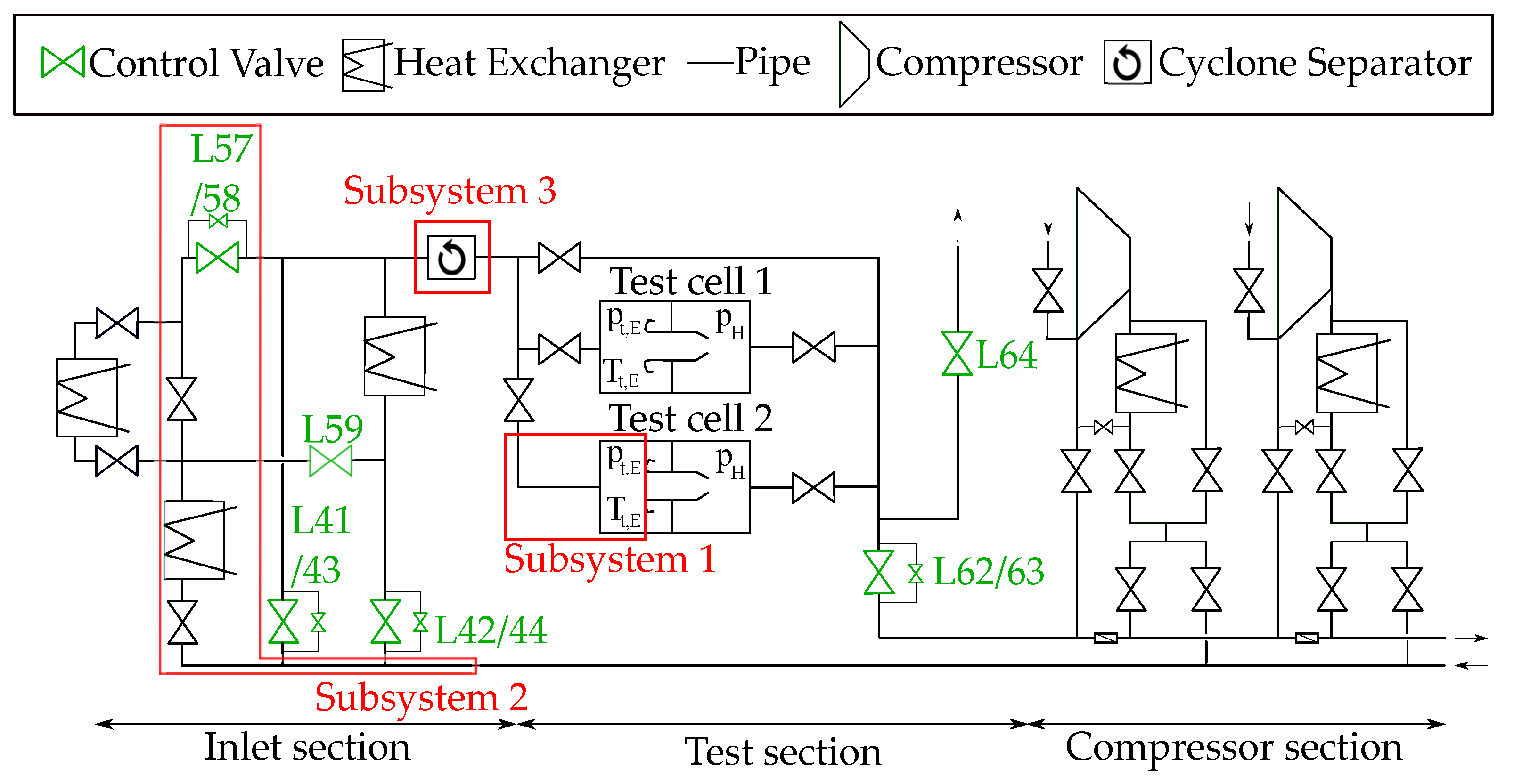
2. Physical Aspects and the Selection of Subsystems for the Stuttgart Altitude Test Facility

The structure of an ATF results from its task which provides the boundary conditions experienced by a test specimen under altitude conditions during ground test operations with a given ambient pressure $p_0$ and ambient temperature $T_0$. The boundary conditions are expressed by altitude pressure $p_H$ at the outlet as well as the total pressure $p_{t,E}$ and total temperature $T_{t,E}$ at the inlet of the test specimen. The relevant combinations of ground and altitude conditions require a variety of thermodynamic processes, which must be provided by the given test-bed. Figure 1 depicts such a system, using the ATF of the University of Stuttgart as an example. The thermodynamic processes are realized through a complex pipe system that connects valves as flow controlling devices with compressors and heat exchangers.

Subsystems

The pipe system consists of numerous pipes with varying lengths and diameters, elbows, and junctions. The pipe system results in complex flow patterns which evolve downstream from the flow path, influencing total pressure losses. An example of this is given with Subsystem 1. Apart from the junctions, Subsystem 1 entails all of the aforementioned components as well as a diffusor and a nozzle. These complex flow patterns also impact the valves acting as the flow control system. With valve characteristics typically being derived from laboratory experiments, a deviation of the actual valve performance is to be expected. These installation effects are relevant for the control design and are discussed using Subsystem 2 as an example. In addition, the size of this type of test facility introduces thermal time constants, which become a limiting factor in the minimum time required to transition between operating points with varying test specimen inlet temperatures. This limitation can best be demonstrated using a subsystem characterized by high mass and wetted surface area. Subsystem 3 serves as an example of this, which is represented by the cyclone separator of the ATF, with a mass of $m_s$ = 32,000 kg and a wetted surface area of $A_i$ = 196 m${}^2$. All subsystems are highlighted by red boxes in Figure 1.

3. Evaluation of the Facility Response

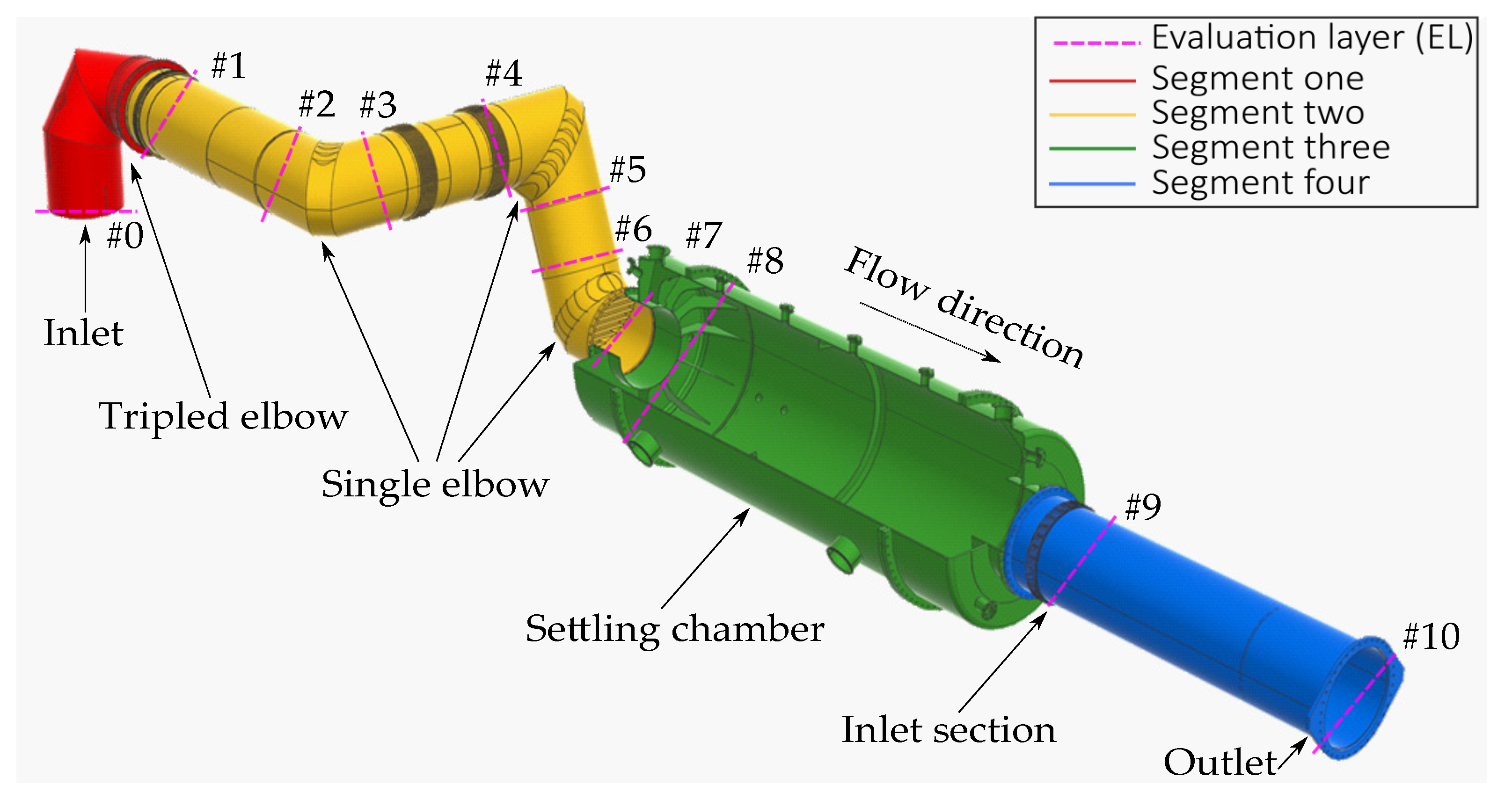
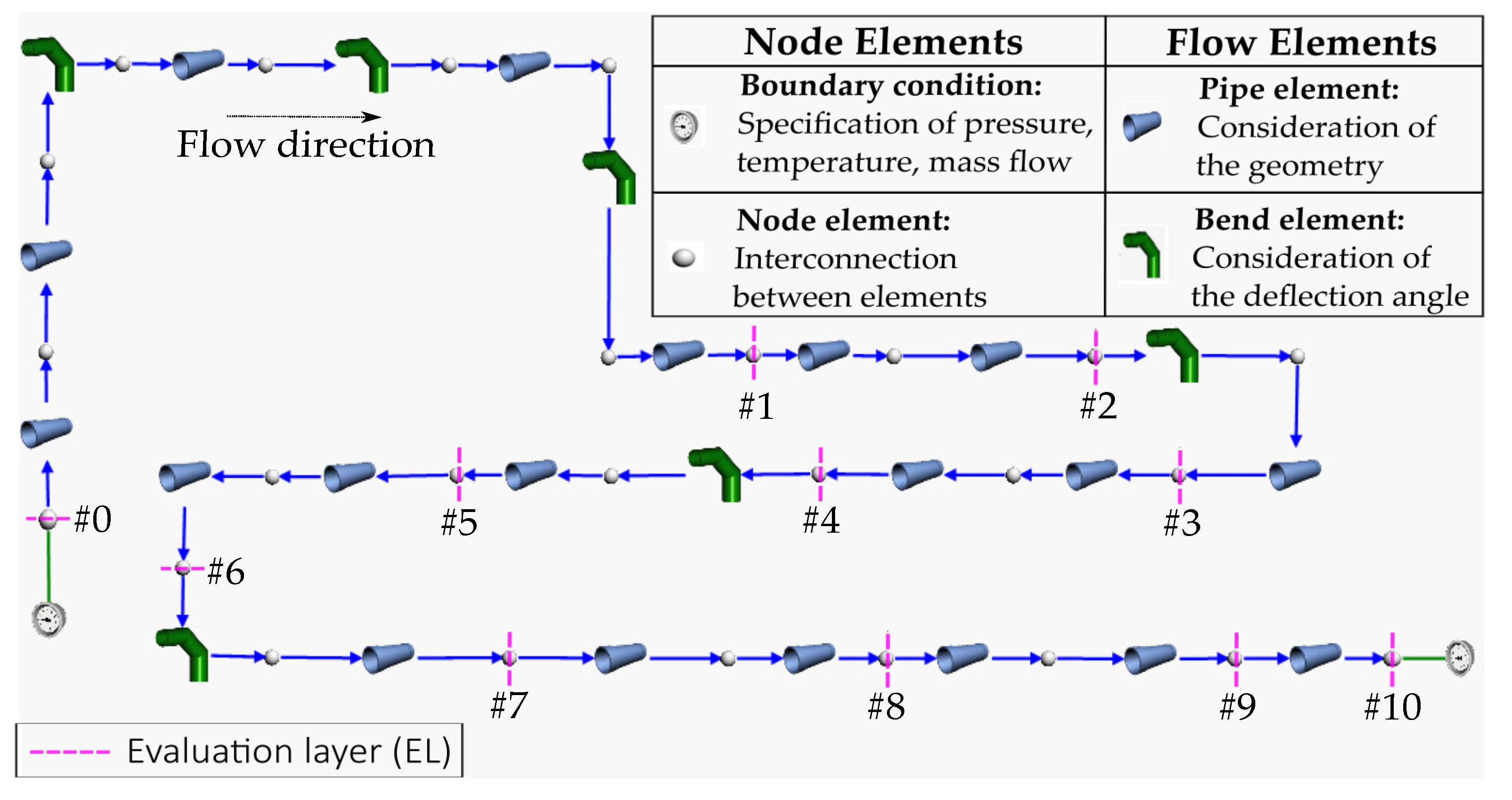
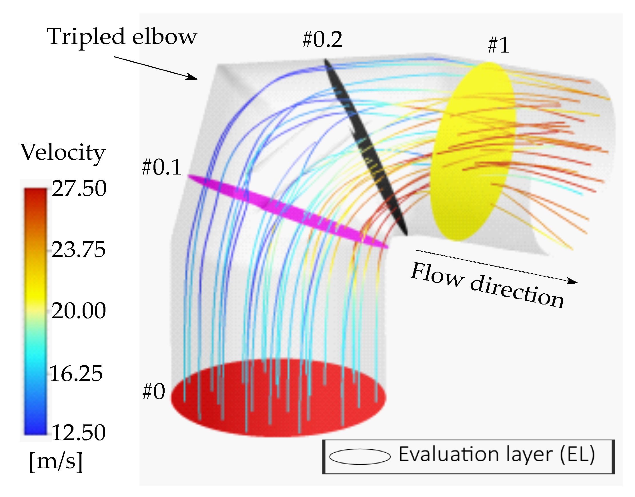
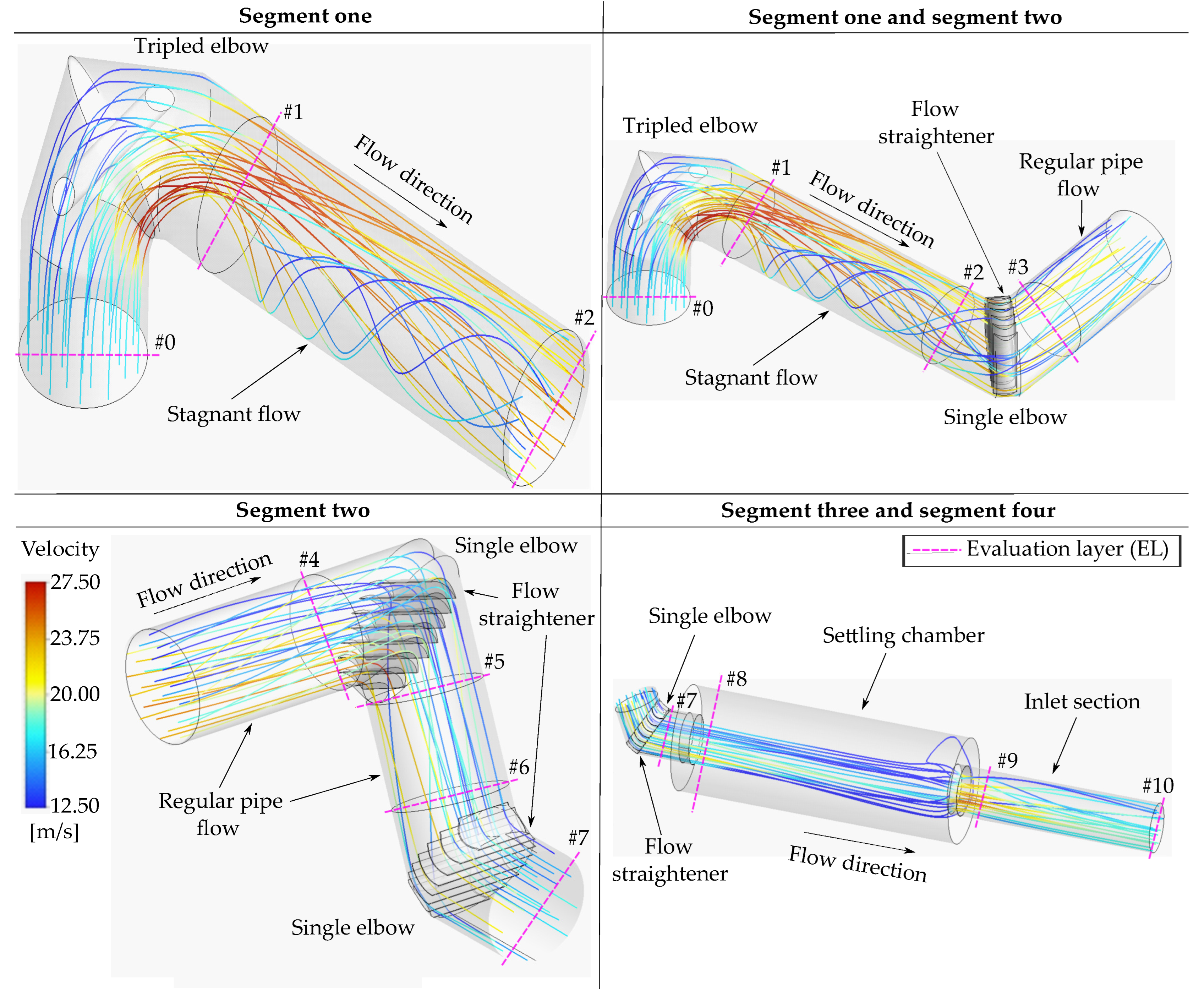
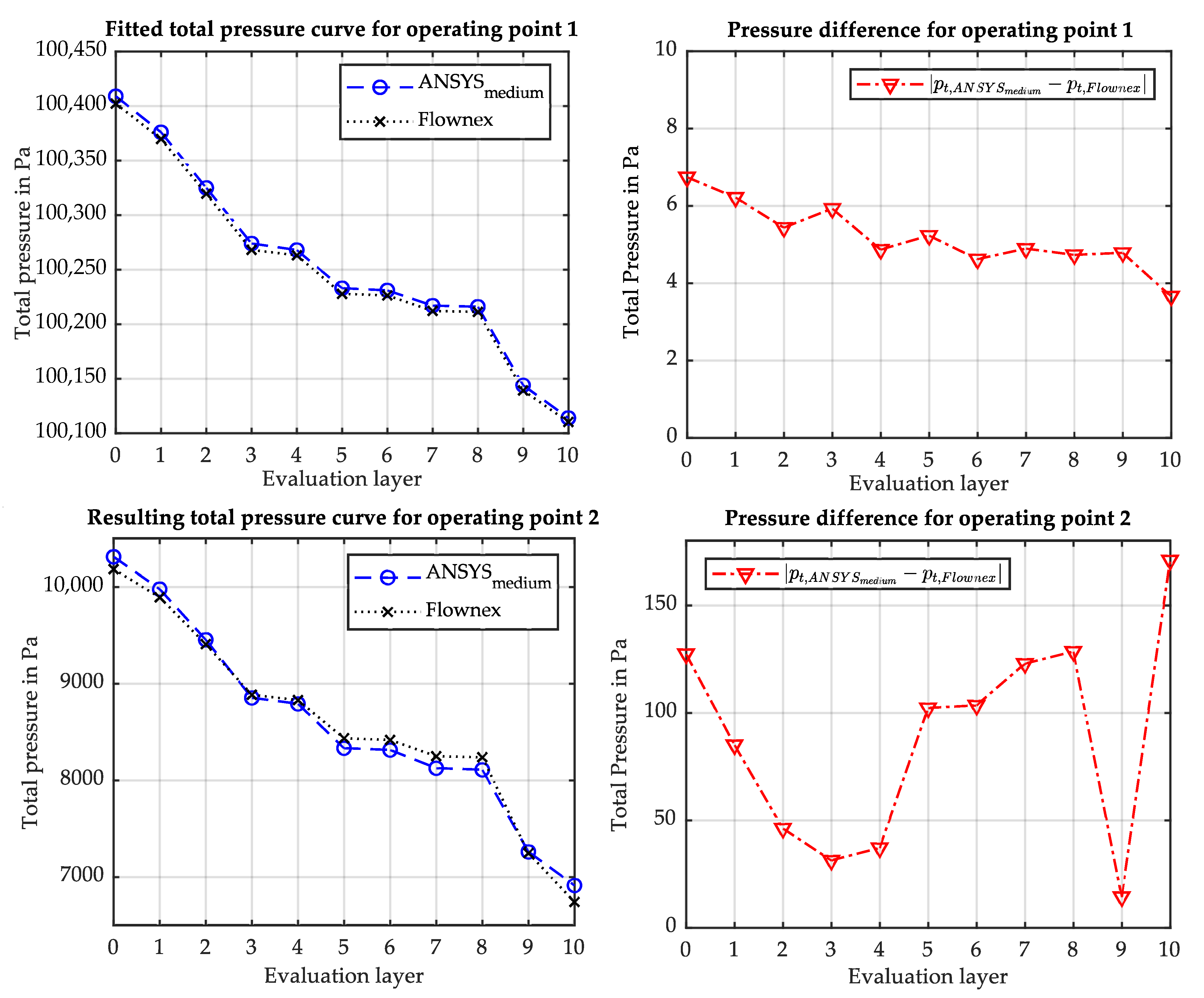
3.1. Subsystem 1—Asymmetric Pipe Flow and Resulting Pressure Losses

Subsystem 1 is shown in Figure 2. It entails all relevant components required to be representative of the ATF pipe system, i.e., elbows, compensators, pipes, a settling chamber, and cross-section changes. Evaluation layers are introduced at a distance of $0.1·D_{Pipe}$ in front or behind a flow disturbance in order to analyze the total pressure losses and the respective flow patterns evolving along the pipe flow. Subsystem 1 is divided into four segments. The first segment is characterized by a tripled elbow with varying deflection angles. The second segment contains single elbows with a constant deflection angle. Both segments have varying pipe lengths and constant pipe diameters. With the integration of a settling chamber, represented by segment three, the diameter abruptly widens up. Finally, the fourth section is the inlet section for the test specimen where the pipe diameter decreases again.

A steady-state, one-dimensional network model of Subsystem 1 has been set up using the commercial software suite Flownex [34]. As shown in Figure 3, the one-dimensional model consists of nodes and flow elements.

Due to its modular nature and wide range of standardized component models, this modeling approach is transferable to other subsystems and test facilities [13,18,26]. The conservation equations of mass and energy are solved at the nodes to derive node pressure and temperature. The node pressure and temperature as well as mass flow are the only parameters coupling adjacent flow elements. As a consequence of the one-dimensional flow computation, there is no information about the flow quality in the elements and the influence of flow quality on the performance of the successive elements is not modeled. Therefore, the one-dimensional computation makes symmetry an inherent feature of the network models. As a result, the pipe and elbow models are limited to a flow that completely fills their cross-sectional area, which excludes by definition typical flow phenomena involving flow separation and re-circulation areas. It must be also noted that the correlations utilized to derive elbow pressure losses as a function of the deflection angle are based on a fully developed pipe flow at the elbow entry [35]. Such a fully developed pipe flow is generally achieved by an adequate flow length, which can be up to 20–30 times the pipe diameter [33]. This is hardly achieved in an ATF pipe system.

In order to understand the quality achieved by the one-dimensional network model, it is necessary to establish a comparison with a reference that closely represents the actual flow within the chosen subsystem. One possibility for this is to conduct in-service measurements with a high level of spatial resolution at the interfaces of the flow elements. Given the limitations in instrumentation commonly encountered in such test facilities, numerical simulations of the flow present a favorable alternative to these measurements.

ANSYS 2022R1 is applied to the geometry shown in Figure 2. The pipe and plenum sections are designed with a structured mesh, while the elbows are generated with an unstructured mesh. Inflation layers at the wall are used and the simulation is performed with wall functions. Mesh convergence studies are performed with mesh sizes of 1 million (coarse), 3 million (medium) and 9 million (fine) cells. Steady-state compressible simulations are performed with second-order accuracy in space. For the turbulent closure, the shear stress transport model is used [36]. Both models are compared at the operating points which are enlisted in

Table 1. Relevant operating points.

Operating Point	Inlet Mass Flow	Turbulence Intensity	Area-Averaged Inlet Total Temperature	Area-Averaged Outlet Static Pressure
-	${\dot{m}}_0$	$T{u}_0$	$T_{t,0}$	$p_{10}$
1	20 $\frac{\mathrm{kg}}{\mathrm{s}}$	3%	455 K	1 bar
2	15 $\frac{\mathrm{kg}}{\mathrm{s}}$	3%	620 K	0.05 bar

. Operating point 1 signifies a standard sea level operation of the test specimen, whereas operating point 2 corresponds to altitude test conditions characterized by the minimum Reynolds number.

For both simulations, the mass flow ${\dot{m}}_0$ and area-averaged total temperature $T_{t,0}$ are defined at the inlet and an area-averaged static pressure $p_{10}$ is set at the outlet. The results for the simulation of operating point 1 are shown in Figure 4.

The grid convergence index (GCI) for the ANSYS simulation [37] is calculated for the total pressure at the inlet (evaluation layer 0). The comparison of the medium and fine grid results in a GCI of 0.9998. As a consequence, the medium mesh size of 3 million cells will be utilized for the continuing discussions. As can be seen in Figure 4, the total pressure drop predicted by the one-dimensional network model significantly exceeds the total pressure drop predicted by the RANS simulation. Both models predict a similar total pressure drop for the pipe elements between evaluation layers 3 and 4 as well as 5 and 6. The total pressure drop of the pipe element between evaluation layers 1 and 2 as well as 9 and 10 is under-predicted by the one-dimensional network model. The total pressure drops for the flow elements between evaluation layers 0 and 1, 2 and 3, 4 and 5 as well as 6 and 8 are over predicted by the one-dimensional network model. It is this over-prediction of the total pressure drops which mainly contributes to the difference between the two models. There are multiple factors contributing to this outcome. The three-dimensional pipe bend between layers 0 and 1 is modeled as a series of two-dimensional bends of a defined degree of flow turning in the one-dimensional network model. The real flow situation depicted in Figure 5 shows that the flow in the combined bend element finds a way of significantly lowering the flow turning between evaluation layers 0.1 and 0.2. The lower degree of flow turning results in a lower total pressure drop. Connected to the deficiency in flow turning is an area of stagnant flow, which is shown in the upper-left picture of Figure 6. The combination of both effects results in a deviation of the flow angle of 5${}^{\circ }$ at the exit of the tripled elbow in association with a highly three-dimensional and turning flow. The detailed flow simulation of the pipe element between layers 1 and 2 results in a three-dimensional flow with high velocity gradients which results in high dissipation and therefore in a higher total pressure drop than the one predicted by the one-dimensional network model.

While the one-dimensional network model over-predicts the total pressure loss for the tripled elbow, the reason for the over-prediction of the pressure losses for the single elbows is different. As can be seen in Figure 6, Subsystem 1 contains flow straighteners between evaluation layers 2 and 3, 4 and 5, and 6 and 7. The effect of a flow straightener is to homogenize the flow and to reduce the pressure losses of the elbows as well as for the succeeding pipe flow. With the elbows between layers 2 and 3 as well as 4 and 5 being identical, the one-dimensional network model predicts identical pressure losses (as can be seen in Figure 4). As shown in Figure 6, the quality of the flow approaching the elbow between 2 and 3 is worse than the flow approaching the elbow between layers 4 and 5. The detailed flow simulation, therefore, predicts differences in the pressure loss (as can be seen in Figure 4). The axial stream lines shown in Figure 6 for the pipe elements between evaluation layers 3 and 4 as well as 5 and 6 indicate regular pipe flow, which results in a good match between the one-dimensional network model and the RANS simulation.

The pressure drop between evaluation layers 7 and 8 calculated by the one-dimensional network model is based on the assumption that the dynamic pressure is completely dissipated in the settling chamber. The detailed flow simulation shown in the lower-right plot of Figure 6 indicates that the flow at evaluation layer 8 is concentrated around the middle axis without a dramatic reduction in flow velocity. This is the reason for the overestimation of the total pressure loss between layers 7 and 8 by the one-dimensional model. The remaining flow inhomogeneities are reflected in the RANS simulation. In comparison to the one-dimensional network model, this leads to a higher total pressure loss between evaluation layers 9 and 10.

The explainable, systematic nature of the above deviations justifies the adjustment of the one-dimensional simulation based on the insights gained from the high-quality RANS simulation. A similar approach is suggested by Sheeley et al. [17] and Liu et al. [25]. The result of such an adjustment is shown in the upper graphs of Figure 7. This is achieved by changing the deflection angles of the Flownex model and secondary loss factors, which are utilized to calculate the pressure losses [35]. The lengths and diameters of the flow elements are not changed in order to maintain geometrical similarity. The difference between the one-dimensional network model and the RANS simulation was minimized for operating point 1. The adjusted one-dimensional model is subsequently utilized to simulate operating point 2 of Table 1 and compared to the three-dimensional RANS simulation.

The pressure difference between the adjusted one-dimensional and the three-dimensional simulation is increased by a factor of 10 for operating point 2 which has a ten times smaller pressure level than operating point 1, indicating the limited applicability of a single operating point adjustment to the wide operating range of the altitude test facility. This is shown in the lower plots of Figure 7.

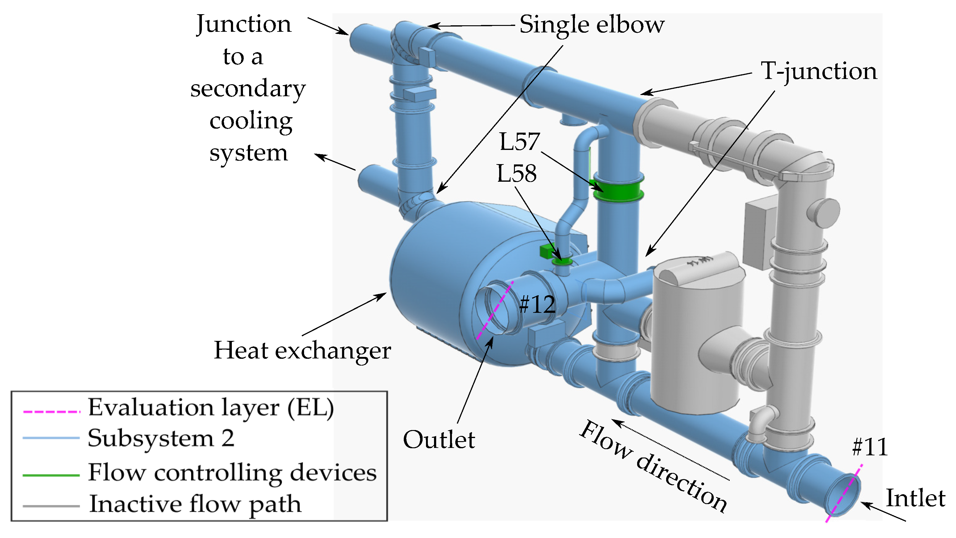
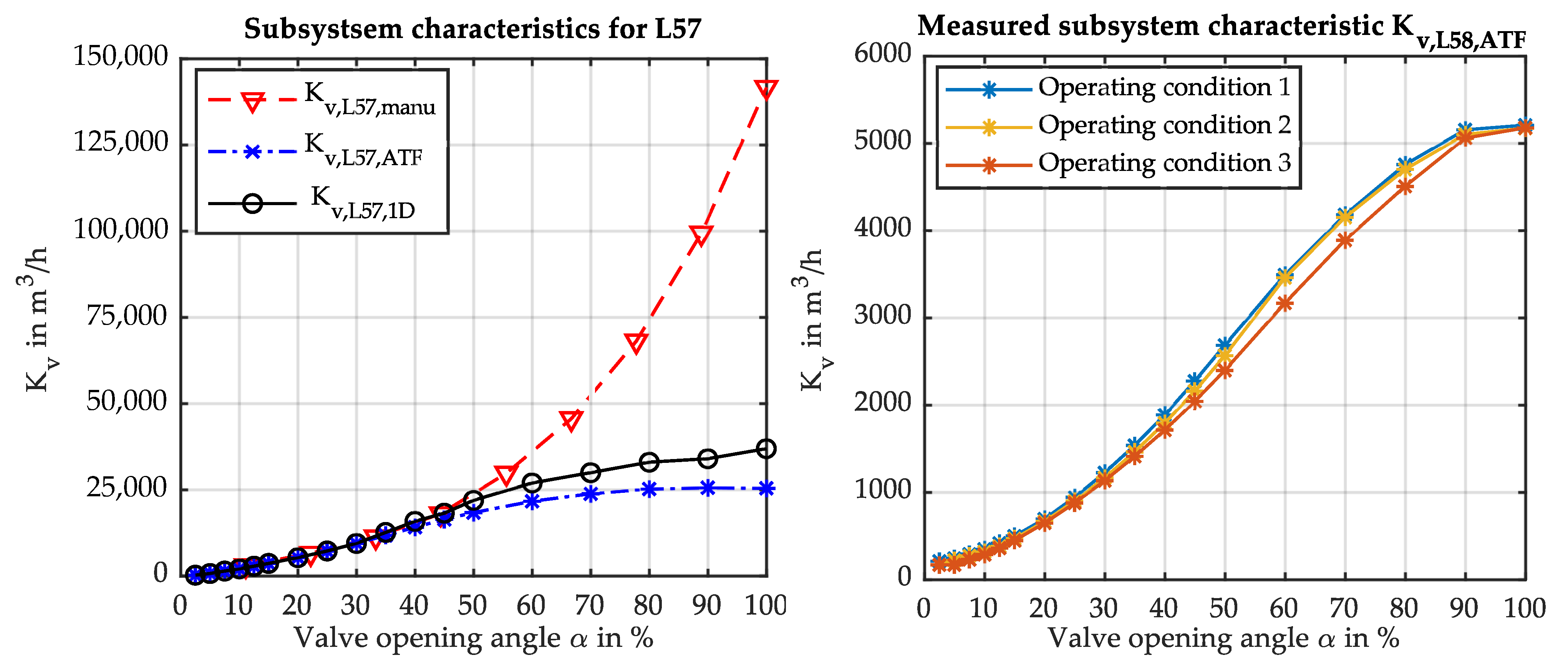
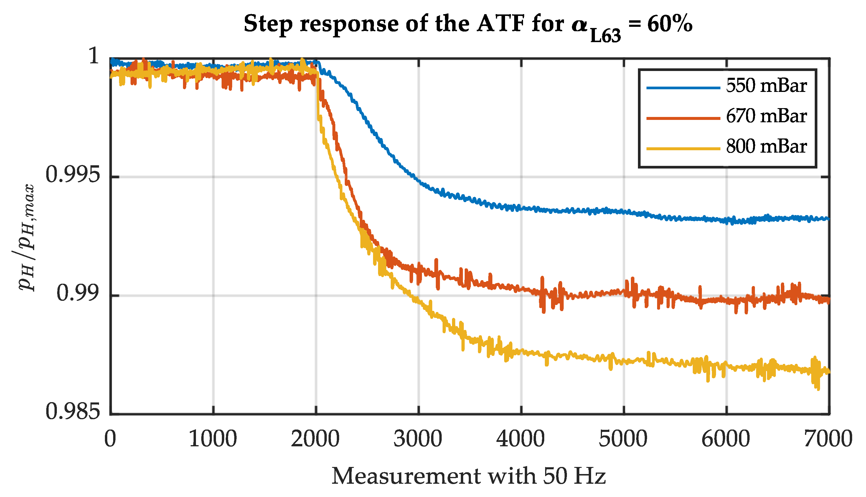
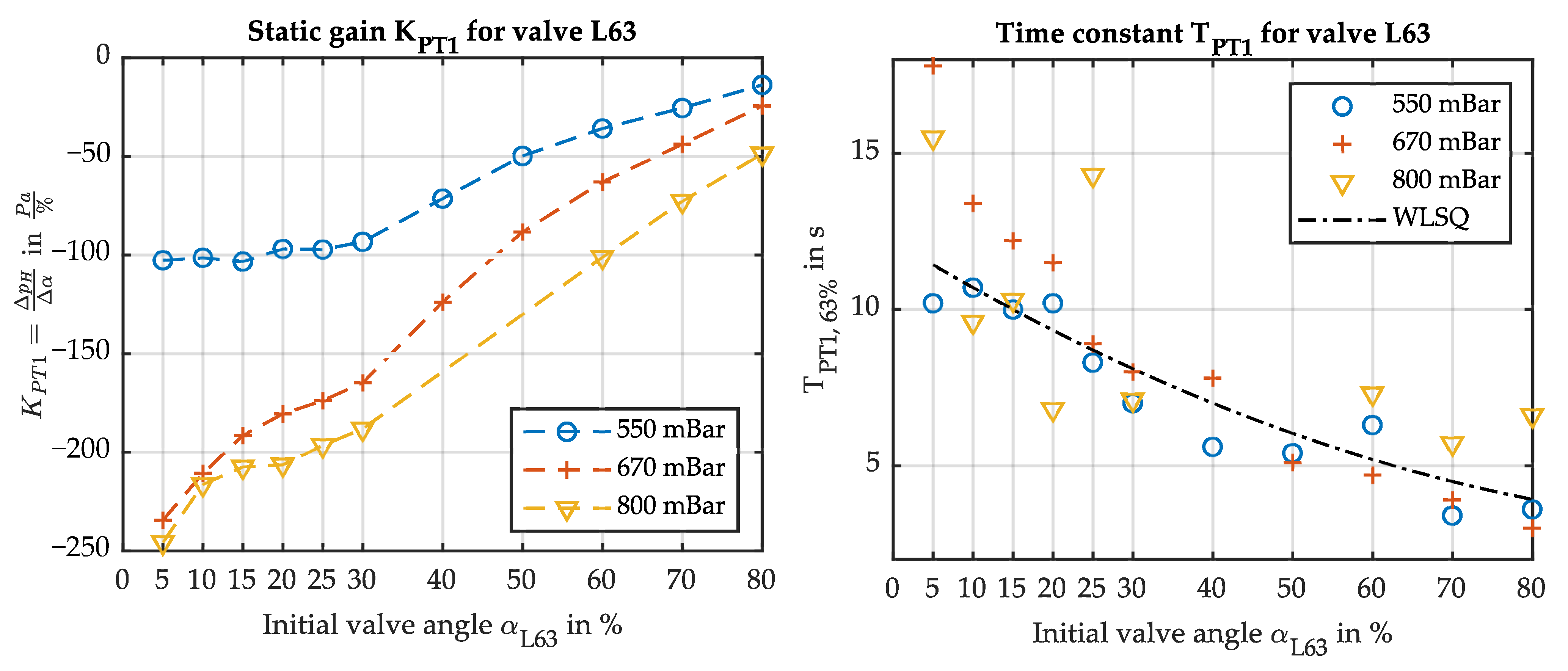
3.2. Subsystem 2—Impact of Asymmetric Flow Phenomena on Flow Control and Subsystem Characteristics

Subsystem 2 is defined between evaluation layers 11 and 12. This is shown in Figure 8. It entails two hydraulic valves acting as flow-controlling devices. Valve L57 is the main valve of large dimension which is used for coarse control. Valve L58 is the bypass valve which is used for fine adjustments. As shown in Figure 8, the flow section upstream and downstream of the control valves L57 and L58 not only features straight pipes, but also elbows, T-junctions, and other junctions. The flow phenomena associated with the elbows and the T-junctions were partly discussed in the previous subsection and comprise asymmetric flow phenomena such as blockage, flow separation, re-circulation areas as well as increased friction [38,39,40,41,42].

The volume flow through a flow controlling valve can be expressed using a subsystem volume flow coefficient $K_v$. In order to quantify the volume flow through a flow-controlling device, pressure and temperature sensors in evaluation layers 11 and 12 are installed. Additionally, the pipe mass flow has been measured during an identification test using a venturi nozzle downstream of evaluation layer 12. The parameter $K_v$ is unique for each active flow controlling device, correlated with the respective valve opening angle $\alpha$ and is calculated as described in Equation (1). A detailed description regarding the calculation and all parameters can be found in [33] or in DIN EN 60534-2-3.

$$\begin{array}{cc}\hfill K_v& =\frac{Q}{N_9·p_{11}·Y·{10}^{-5}·\sqrt{\frac{x}{M·T_{11}}}},Q=\frac{\dot{m}}{{\rho }_0}·3600\frac{\mathrm{s}}{\mathrm{h}}\hfill \\ \hfill x& =\frac{p_{11}-p_{12}}{p_{11}},Y=1-\frac{x}{3}\hfill \\ \hfill N_9& =2.46·{10}^3\mathrm{m}{\mathrm{s}}^2\sqrt{\frac{\mathrm{K}}{\mathrm{g}\mathrm{mol}}},M=28.96\frac{\mathrm{g}}{\mathrm{mol}}\hfill \\ \hfill R_s& =287.058\frac{\mathrm{J}}{\mathrm{kg}\mathrm{K}},{\rho }_0=1.2922\frac{\mathrm{kg}}{{\mathrm{m}}^3}\hfill \end{array}$$

(1)

In the left plot of Figure 9, the measured subsystem characteristic of the main valve L57 $K_{v,L57,ATF}$ is depicted in blue. It is significantly different from the characteristic supplied by the valve manufacturer $K_{v,L57,manu}$, which is shown in red. The difference starts to increase at an opening angle of $\alpha >{40}^{\circ }$. In contrast to the measured subsystem characteristic $K_{v,L57,ATF}$, the manufacturer’s valve characteristic $K_{v,L57,manu}$ is tested in a laboratory situation which ensures fully developed pipe flow in front and after the valve. Hence, the valve is the flow-restricting element at all mass flows and its characteristic does not level out at high valve-opening angles. It is the above-mentioned installation effects that make the measured subsystem characteristic $K_{v,L57,ATF}$ level out with an increase in the valve-opening angle. The actual flow capability of Subsystem 2 is dominated by the pipe system instead of the flow control valve in this area.

The subsystem volume flow coefficient $K_v$ is evaluated in the one-dimensional-network model, as the subsystem characteristic is essential for the simulation-based testing and validation of control concepts. This is realized by matching the one-dimensional model of Subsystem 2 with the measured values at evaluation layers 11 and 12. The measured inlet pressure $p_{11}$, the measured inlet temperature $T_{11}$, and the measured mass flow ${\dot{m}}_{12}$ are specified as fixed-boundary conditions. The volumetric flow coefficient in the one-dimensional model $K_{v,1D}$ is adjusted such that the simulated outlet pressure matches the measured outlet pressure $p_{12}$. Consequently, the simulated subsystem flow coefficient $K_{v,1D}$ comprises all model deviations and is depicted in black in the left plot of Figure 9. The difference in the measured subsystem volume flow coefficient $K_{v,L57,ATF}$ and the simulated one $K_{v,1D}$ indicates the inaccuracy of the one-dimensional model in predicting the installation effects at opening angles of $\alpha >{40}^{\circ }$ in the one-dimensional network model.

As the flow phenomena and consequently the subsystem volume flow coefficient $K_v$ depend on the operating conditions, the right plot of Figure 9 shows the measured subsystem volume flow coefficient for L58 $K_{v,L58,ATF}$ for three different operating conditions. The dependency of $K_{v,L58,ATF}$ on the operating conditions for the flow-controlling devices supports the argument of Section 3.1 that the adaptation of a one-dimensional network model to a single operating condition is insufficient based on the wide operating range of an ATF and the associated changes in subsystem characteristics.

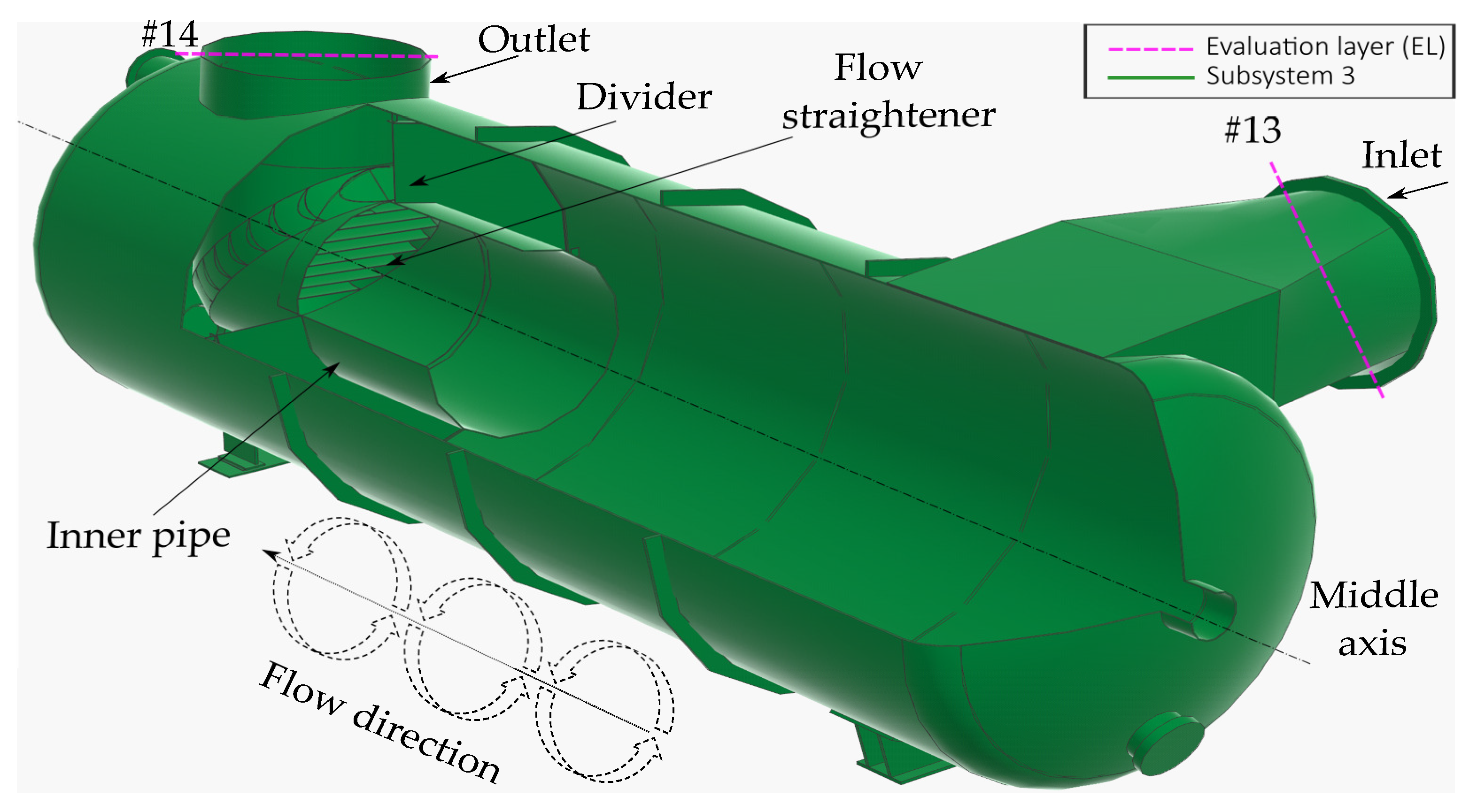
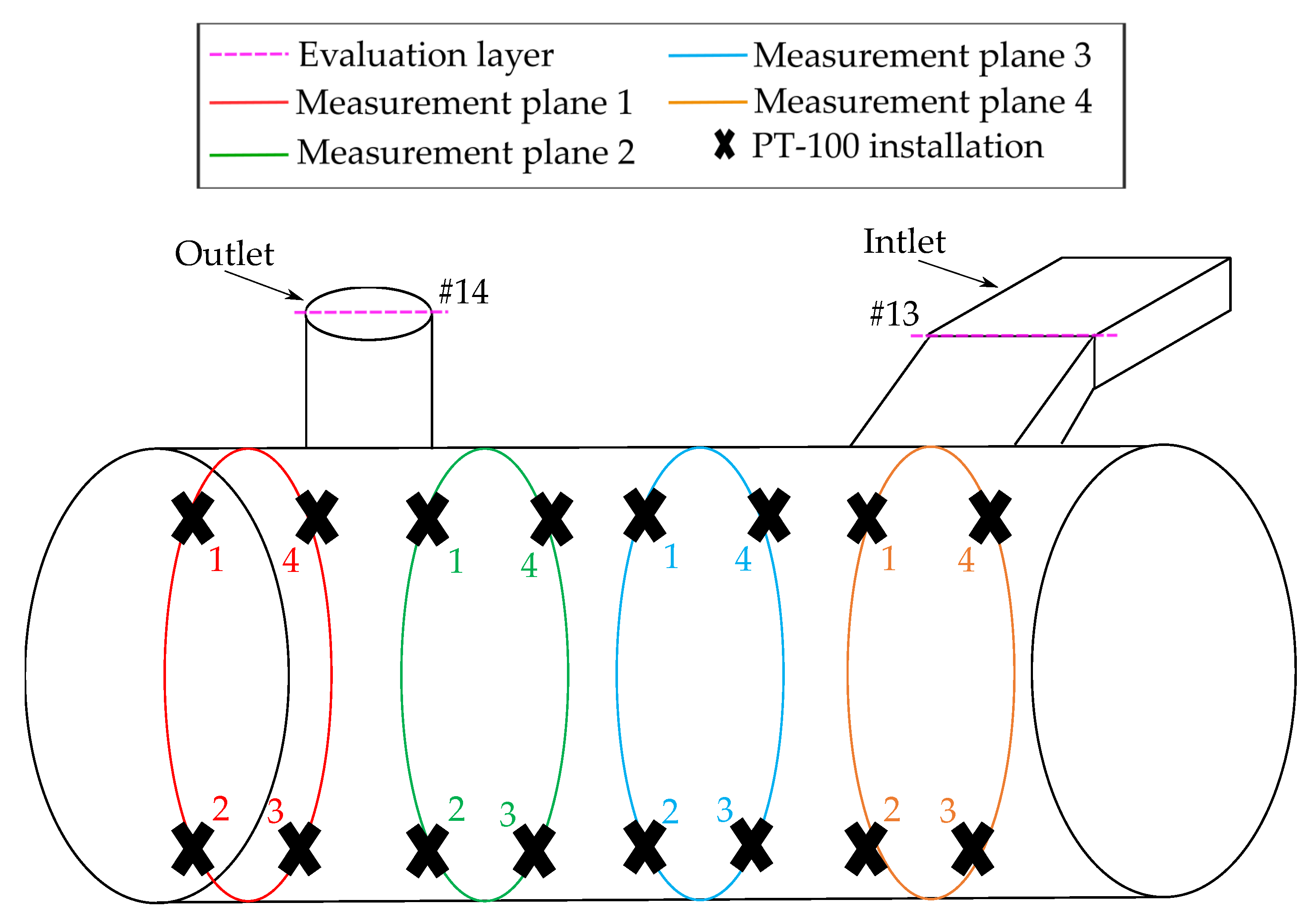
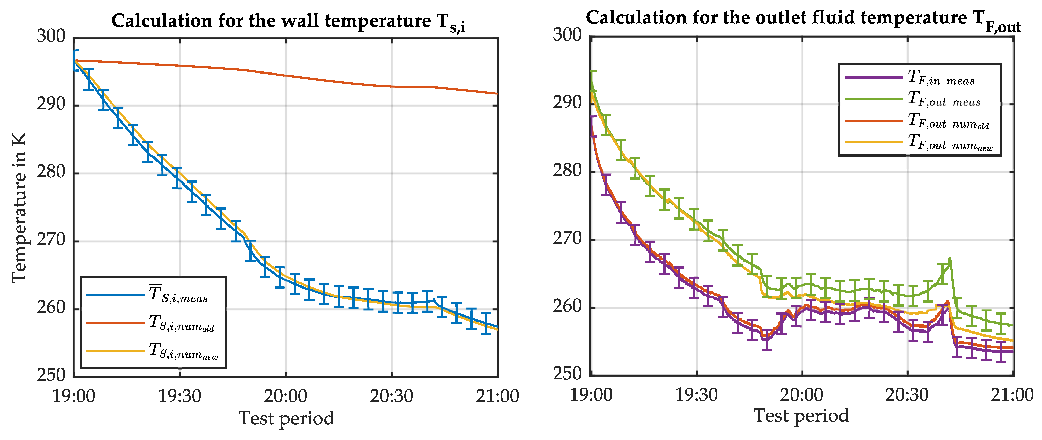
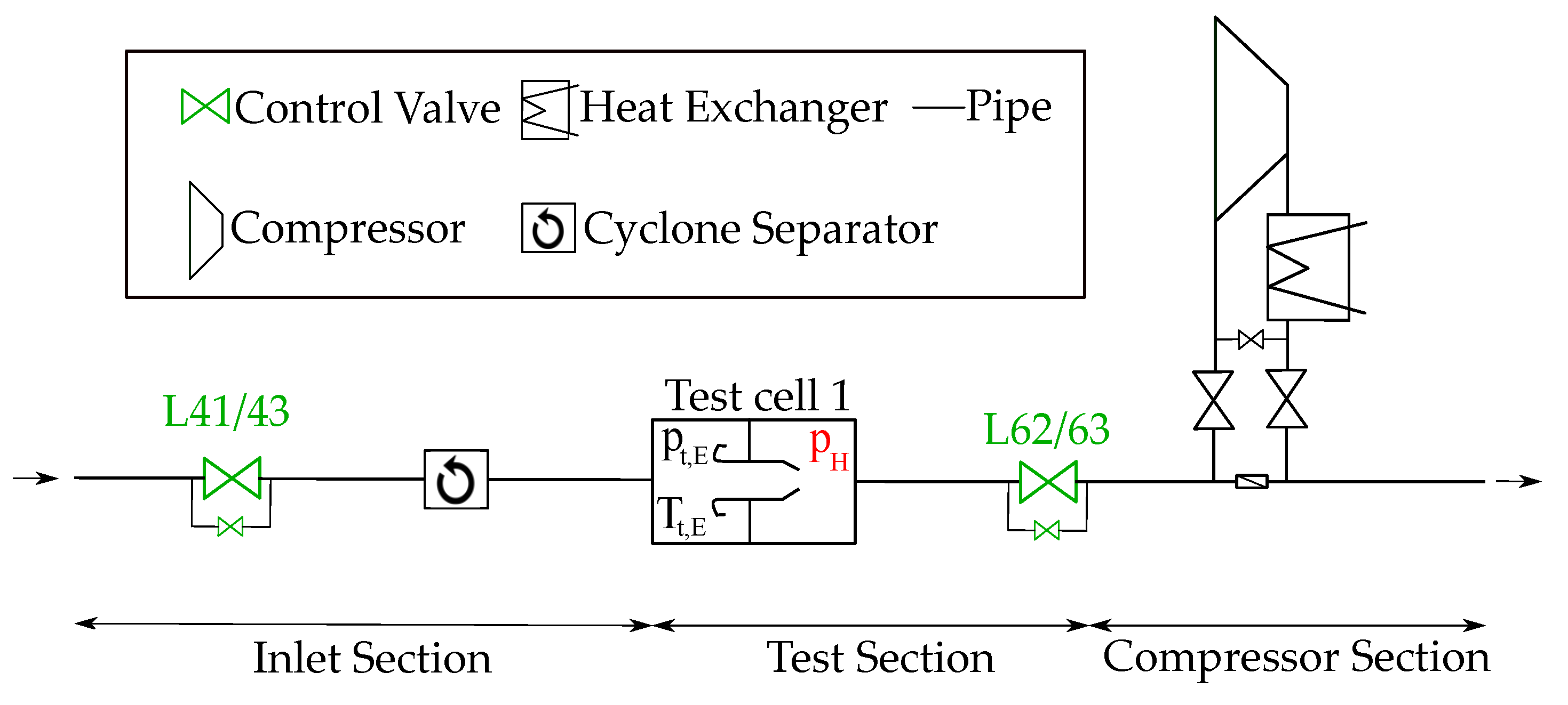
3.3. Subsystem 3—Cyclone Separator and Heat Transfer

Subsystem 3 is defined between evaluation layers 13 and 14. This is shown in Figure 10. Subsystem 3 is a cyclone separator in front of test cells 1 and 2 which is utilized to separate potential harmful debris from the working fluid. With a total mass of $m_s$ = 32,000 kg and a wetted surface area of $A_i=196{\mathrm{m}}^2$, the cyclone separator plays a vital role in terms of heat transfer and has a lasting impact on the temperature of the exiting working fluid which leads to thermal time constants in the test cell. The air enters the cyclone separator at the evaluation layer 13 and circulates along the middle axis. While the working fluid passes the inner pipe through a flow straightener and is led through evaluation layer 14 to the respective test cell, the debris passes a divider and is collected. No thermodynamic process takes place from evaluation layer 13 up to the entry of the test cell. Based on the relevance of Subsystem 3 for heat transfer, it is analyzed to demonstrate the challenges for the implementation in the network model. Due to the one-dimensional, symmetric nature of the model, the equations for mass, energy, and momentum conservation are solved with no spatial dependence [3,13,23,25]. This assumption results in ordinary differential equations instead of complicated partial differential equations and is applied to cope with computational, feasibility, and time constraints [3,17,43].

Moreover, this leads to a homogeneous distribution in the considered control volume, here represented by Subsystem 3. It inherits one representative value for temperature and pressure. Additionally, the conservation equations lead to calculations for changes in pressure and temperature based on an absolute value for the heat transfer $\dot{Q}$ which needs to be determined.

The heat transfer ${\dot{Q}}_i$ from the working fluid of temperature $T_F$ to the cyclone separator structure of temperature $T_{s,i}$ is defined by Equation (2). The fluid temperature $T_F$ is the mean value between the inlet temperature $T_{F,in}$ and the outlet temperature $T_{F,out}$. Equation (2) depends on the wetted surface $A_i$, the heat transfer coefficient ${\alpha }_i$ [44,45,46] and the temperature difference. The heat transfer on the outside ${\dot{Q}}_a$ is neglected due to insulation [47].

$${\dot{Q}}_i\left(t\right)={\alpha }_i\left(t\right)·A_i·(T_{s,i}\left(t\right)-T_F\left(t\right))$$

(2)

As can be seen in Equation (2), the heat transfer ${\dot{Q}}_i$, the heat transfer coefficient ${\alpha }_i$, and the temperatures $T_{s,i}$ and $T_F$ are functions of time. Moreover, by considering Equation (3), the time dependency of the calculated outlet temperature $T_{F,out}$ is a function of the fluid temperature $T_F$ and a term describing the time delay associated with the heat transfer to the structure and the incoming fluid flow. The term depends on the mass flow $\dot{m}$, which is highly reliant on the test specimen and the operating point of the ATF.

$$T_{F,out}\left(t\right)=T_F\left(t\right)·\left(1-\frac{{\dot{Q}}_i\left(t\right)}{T_F\left(t\right)·\dot{m}\left(t\right)·c_p}\right)$$

(3)

While pressure changes propagate at the speed of sound and therefore with minimal time delay, the time dependency of Equations (2) and (3) raises the question of the relevance of thermal time constants $\tau$ for the one-dimensional network model. In order to assess the magnitude of time delay, an area and mass equivalent pipe of Subsystem 3 with axial flow is considered. This is shown in the left picture of Figure 11. A step change in the inlet temperature $T_{F,in}$ is forced onto the system in order to estimate the delay in the outlet temperature $T_{F,out}$. The thermal time constant $\tau$ shall be defined by the time the calculated outlet fluid temperature $T_{F,out}$ takes to converge to 95% of the forced inlet fluid temperature $T_{F,in}$ [12]. The heat transfer coefficient is chosen to be constant for now and follows representative values for forced convective flow [44].

In order to calculate the heat transfer ${\dot{Q}}_i$ based on Equation (2), the change in the wall temperature ${\dot{T}}_{s,i}\left(t\right)$ is evaluated as shown in Equation (4). The parameter $c_s$ represents the specific heat capacity of the material.

$${\dot{T}}_{s,i}\left(t\right)=\frac{-{\dot{Q}}_i\left(t\right)}{m_s·c_s}$$

(4)

The results of the calculation are shown in the right plots of Figure 11. It is apparent, that an increased mass flow $\dot{m}$ not only reduces the time constant ${\tau }_{\#,95\%}$, but also leads to a greater immediate step on the outlet temperature $T_{F,out}$. The choice of the constant heat transfer coefficient ${\alpha }_i$ makes the impact of the increased average fluid temperature on the heat transfer to the structure visible. Higher mass flows lead to higher average fluid temperatures and result in a faster heating up of the structure. The thermal time constants ${\tau }_{\#,95\%}$ for mass flows of $\dot{m}=15 \frac{\mathrm{kg}}{\mathrm{s}}$, $\dot{m}=50 \frac{\mathrm{kg}}{\mathrm{s}}$, and $\dot{m}=100 \frac{\mathrm{kg}}{\mathrm{s}}$ are listed in

Table 2. Thermal time constants ${\tau }_{\#,95\%}$ for the course of the outlet temperature.

Mass Flow $\dot{\mathit{m}}$	Thermal Time Constant ${\mathit{\tau }}_{\#,95\%}$
$\dot{m}=100 \frac{\mathrm{kg}}{\mathrm{s}}$	${\tau }_{1,95\%}$ = 1829 s
$\dot{m}=50 \frac{\mathrm{kg}}{\mathrm{s}}$	${\tau }_{2,95\%}$ = 2787 s
$\dot{m}=15 \frac{\mathrm{kg}}{\mathrm{s}}$	${\tau }_{3,95\%}$ = 5763 s

.

As a next step, a suitable correlation for the heat transfer coefficient ${\alpha }_i$ must be determined. This requires a comparison with the metal temperatures of the subsystem structure. For this purpose, the inner surface of Subsystem 3 is equipped with a total of sixteen PT-100 sensors, installed in accordance with the guidelines provided by [48]. Four sensors each have been evenly distributed across each measurement plane, as illustrated in Figure 12.

In terms of the heat transfer coefficient, Equation (5) is utilized, in which the heat transfer coefficient is calculated based on the inner pipe diameter $D_i$, the thermal conductivity ${\lambda }_F$ of the fluid, and a suitable Nusselt number $Nu$.

$${\alpha }_i=\frac{Nu·{\lambda }_F}{D_i}$$

(5)

The Nusselt number $Nu$ is calculated with an associated correlation. The correlation for forced convection generally depends on the Reynolds number $Re$ and the Prandtl number $P{r}_F$. The calculation of the Reynolds number is shown in Equation (6).

$$Re=\frac{4·\dot{m}}{\pi ·D_i·{\eta }_F}$$

(6)

Look-up tables for dry air [44] are applied to calculate the dynamic viscosity ${\eta }_F$, the thermal conductivity ${\lambda }_F$, and the Prandtl number $P{r}_F$, based on the temperature $T_F$. There is a set of Nusselt correlations from which a suitable correlation has to be chosen [44,45,46,48]. It turns out that Nusselt correlations for axial pipe flow underestimate the heat transfer in Subsystem 3 [47]. This is shown in the left of Figure 13 where a test campaign with a low inlet fluid temperature $T_{F,in,meas}$ is utilized. The average surface temperature over all measurement planes ${\overline{T}}_{s,i,meas}$, depicted in blue, is compared to the calculated wall temperature based on Nusselt correlations for axial pipe flow [47]$T_{s,i,nu{m}_{old}}$, as illustrated by the orange line. The heat transfer is underestimated, and as a consequence, the wall temperature does not cool down as measured. Due to the fact that the air flow is not axial in the cyclone separator, such correlations are not applicable. Gaddis [49] introduced a calculation for the Nusselt number for turbulent radial flow on the example of continuous stirred-tank reactors. Since Weisser [47] showed that the flow in the ATF at the University of Stuttgart is permanently turbulent for the relevant operating range, Equation (7) from Gaddis is applied to utilize a new Nusselt correlation for the cyclone separator.

$$Nu=C·R{e}^{2/3}·P{r}_F^{1/3}·{\left(\frac{{\eta }_F}{{\eta }_s}\right)}^{0.14}$$

(7)

The constant C captures the geometric influence and is an adjustable constant parameter. The dynamic viscosity ${\eta }_s$ is calculated via the look-up table based on the calculated wetted surface temperature. This leads to a significantly improved heat transfer prediction. This can be seen in the left graph of Figure 13, as the new calculated wall temperature $T_{s,i,nu{m}_{new}}$, outlined in yellow (based on Equation (7)), more closely matches the average measured wall temperature ${\overline{T}}_{s,i,meas}$.

As shown in the right plot of Figure 13, the heat transfer calculation is further validated by comparing the measured outlet fluid temperature $T_{F,out,meas}$, depicted in green, to a calculated outlet fluid temperature based on the old correlation $T_{F,out,nu{m}_{old}}$ and the new correlation $T_{F,out,nu{m}_{new}}$ following Equation (3). The new Nusselt correlation leads to significantly improved predictions in the measured fluid outlet temperature $T_{F,out,meas}$ which enables the possibility of analytically estimating thermal time constants. The remaining deviation to the measurement can be explained by a non-symmetric incident flow of the sensor measuring the outlet temperature $T_{F,out,meas}$. A combined uncertainty band of $\pm 1.5K$ is depicted in both graphs of Figure 13 based on the measurement uncertainty of the temperature sensors and the analog input modules. It turns out that the dynamics of an ATF are dominated by the fast changes in pressure and a significant time delay in temperature. The control of such a system requires the accurate modeling of the associated time constants across a wide range of operating conditions.

4. System Identification

The complex flow patterns in the ATF pipe work and the nonlinear subsystem characteristics of the flow-controlling elements limit the applicability of a one-dimensional network model which is only adapted to a single operating point. Moreover, such a one-dimensional network model needs to accurately model the subsystem time constants over a wide range of operating conditions. Its limited capability to extrapolate to diverse operating conditions typical to ATF operation makes it directly compete with more data-driven methods such as experimental system identification. A common approach for experimental system identification is the excitation of the system using a Heaviside-function $\sigma \left(t\right)$ [12]. The step change at the ATF is realized by a defined change in control valve position. The system identification comprises the pure flow through the ATF which is operated in suction mode. This mode is depicted in Figure 14.

The control valves upstream of the test chamber L41 and L43 are kept in a constant position. The system response has been tested at a constant opening position of valve L62 and a superimposed step change in the valve position L63. The magnitude of the step change was chosen to be in the region of the measurement frequency in order to ensure the instantaneous change as required by the Heaviside-function $\sigma \left(t\right)$. An exemplary time response in the test chamber static pressure $p_H$ is shown in Figure 15 for a step change from the initial valve opening of ${\alpha }_{L63}=60\%$ for three different test chamber pressure levels $p_H$. The change in the test chamber static pressure $p_H$ shows a dependency on the operating conditions as discussed in Section 3 and corresponds to the dynamics of a proportional–integral–time-delay (PT1) transfer function $h\left(t\right)$.

This is a common mathematical model used to describe the behavior of first-order dynamic systems. For the time-based analysis of the test chamber static pressure $p_H$, the transfer function $h\left(t\right)$ can be written in the time domain. This representation is shown in Equation (8).

$$h\left(t\right)=K_{PT1}·\left(1-e^{\frac{t}{T_{PT1}}}\right)=\frac{\Delta p_H}{\Delta \alpha }·\left(1-e^{\frac{t}{T_{PT1}}}\right)$$

(8)

As can be seen in Equation (8), the transfer function depends on a time constant $T_{PT1}$ and a static gain $K_{PT1}$. The time constant $T_{PT1}$ is defined as the time required for the system to respond to the forced step change in the valve angle ${\alpha }_{L63}$ and reach about 63.2% of the new steady-state test chamber pressure $p_H$. The static gain $K_{PT1}$ indicates the change in the test chamber pressure $p_H$ in correlation with the forced step change in the valve angle ${\alpha }_{L63}$ when the system reaches its steady state [12]. Both values were evaluated for different levels of the test chamber static pressure $p_H$. The time constants $T_{PT1}$ and the static gains $K_{PT1}$ are a function of the starting position ${\alpha }_{L63}$. Figure 16 therefore shows the two constants for varying starting angles ${\alpha }_{L63}$ and test chamber pressure levels $p_H$.

The nonlinear interaction between the compressor and control valve moves the valve operating points to steeper parts of their basic flow through characteristics resulting in decreasing static gains $K_{PT1}$ with an increasing valve opening angle ${\alpha }_{L63}$. The static gains also decrease with a decreasing test cell pressure $p_H$. The decreasing effectiveness with increasing valve angles ${\alpha }_{L63}$ can be observed for the time constant as well. However, as can be seen in the right plot of Figure 16, the time constants show similar behaviors for all pressure levels. That is why a weighted least square method (WLSQ) is applied to determine a quadratic balancing function. Based on the fact that the static gain is highly dependent on the valve angle ${\alpha }_{L63}$ as well as the operating condition, it can be concluded that a classic PID–controller with constant gains $K_P$, $K_I$, and $K_D$ is insufficient for a stable and performing control of the test chamber static pressure $p_H$. Moreover, the balancing function for the time constants shows the same result, which implies a varying inertia of the system response. As a result, advanced control concepts are necessary in order to satisfy stability and controller performance. One common method in this field is gain-scheduling, wherein the constant gains of a PID-controller change with the operating condition [50]. The identified transfer function $h\left(t\right)$ can be transformed to the frequency domain $G\left(S\right)$ and the classical controller design can be applied in order to satisfy stability and performance for each identified operating point [51]. All in all, the system identification forms a transparent, easy-to-compute, and robust model which per definition embraces the complex flow phenomena in the pipe system and the nonlinear characteristics of the flow controlling elements. However, the system identification necessitates a vast amount of test times and datasets. Instead of identifying the whole envelope of the ATF, the future challenge is to identify and specify relevant operating points and apply the aforementioned methods.

5. Discussion

It turns out that the performance of an ATF is the result of the complex interaction of many nonlinear phenomena. The numerical methods of high spatial and time resolution allow the understanding of the interaction of flow phenomena in the complex pipe works. It is only upon this foundation that one-dimensional network models can be understood and optimized. However, it turns out that matching those one-dimensional models to a higher-order model in one operating point is not sufficient. This situation is exacerbated by the nonlinear characteristics of the flow-controlling devices. These characteristics need to be understood in detail to allow sensible one-dimensional modeling. Otherwise, the assignment of the calibration factors cannot be physically justified. The system dynamics are dominated by two phenomena of different response times. These are pressure changes in the ATF volume and heat transfer between the fluid and the ATF structure. All this gives the impetus to apply an experimental system identification in order to derive a basic transfer function. It has been shown that this is a promising and versatile approach to describe the system behavior. However, the interpretation of the resulting time constants and static gains requires an in-depth understanding of all the aspects discussed above. The insights gained from the experimental system identification can be used to derive insights for adequate controller design. The dependency of static gains and time constants of the first-order transfer function on the operating point and the valve angle imply that advanced control concepts are essential.

References

1. EASA CS-E Certification Specification for Engines. Available online: https://www.easa.europa.eu/sites/default/files/dfu/agency-measures-docs-certification-specifications-CS-E-CS-E_Amendment-2.pdf (accessed on 31 August 2023).
2. FAA AC 33-2C: General Type Certification Guidelines for Turbine Engines. Available online: https://www.faa.gov/documentLibrary/media/Advisory_Circular/AC_33-2C.pdf (accessed on 31 August 2023).
3. Köcke, S. Simulation eines Höhenprüfstands zur Untersuchung der Verdichter-Pumpverhütungsregelung. Ph.D. Thesis, University of Stuttgart, Stuttgart, Germany, 2010. [Google Scholar]
4. Roberts, J.; Beyerly, W.; Mason, M.; Glazier, J.; Wiley, R. PW4084 Engine Testing in Altitude & Sea Level Test Facilities. SAE Trans. 1994, 103, 2116–2130. [Google Scholar]
5. Adolf, M. More Energy Efficiency through Process Automation; ZVEI-Zentralverband Elektrotechnik und Elektronikindustrie eV: Frankfurt am Main, Germany, 2012; pp. 1–16. Available online: https://www.zvei.org/fileadmin/user_upload/Presse_und_Medien/Publikationen/2013/januar/More_energy_efficiency_through_process_automation/ZVEI_Energienutzung-englisch.pdf (accessed on 31 August 2023).
6. Luppold, R.H.; Meisner, R.; Norton, J.M. Design and Evaluation of an Auto-Tuning Control System for an Altitude Test Facility. In Proceedings of the ASME 1999 International Gas Turbine and Aeroengine Congress and Exhibition, Manufacturing Materials and Metallurgy; Ceramics; Structures and Dynamics; Controls, Diagnostics and Instrumentation, Indianapolis, IN, USA, 7–10 June 1999; Volume 4. [Google Scholar] [CrossRef]
7. Karpuk, S.; Elham, A. Comparative study of hydrogen and kerosene commercial aircraft with advanced airframe and propulsion technologies for more sustainable aviation. Proc. Inst. Mech. Eng. Part J. Aerosp. Eng. 2023, 237, 2074–2091. [Google Scholar] [CrossRef]
8. Schiewe, C.; Neuburger, N.; Staudacher, S. How Future Propulsion Systems Influence Future Component Testing: Latest Results from Stuttgart Univerity’s Altitude Test Facility. In Proceedings of the Global Power and Propulsion Society Technical Conference, Zurich, Switzerland, 16–17 January 2019. [Google Scholar] [CrossRef]
9. Richter, H. Advanced Control of Turbofan Engines; Springer Science + Business Media, LLC: New York, NY, USA, 2012; pp. 51–226. ISBN 978-1-4614-1170-3. [Google Scholar]
10. Bierkamp, J.; Köcke, S.; Staudacher, S.; Fiola, R. Influence of ATF Dynamics and Controls on Jet Engine Performance. In Proceedings of the ASME Turbo Expo 2007: Power for Land, Sea, and Air. Volume 1: Turbo Expo 2007, Montreal, QC, Canada, 14–17 May 2007; pp. 105–113. [Google Scholar] [CrossRef]
11. Schiewe, C.; Staudacher, S.; Elter, M. Automation of Stuttgart Universitys multi-functional Altitude Test Facility. In Proceedings of the 24th International Symposium on Air Breathing Engines (ISABE), Canberra, Australia, 22–27 September 2019; pp. 733–742. [Google Scholar]
12. Lunze, J. Regelungstechnik 1, 12th ed.; Springer: Berlin, Germany, 2020; pp. 41–233. ISBN 978-3-662-60745-9. [Google Scholar]
13. Montgomery, P.; Burdette, R.; Krupp, B. A real-time turbine engine facility model and simulation for test operations modernization and integration. In Proceedings of the ASME Turbo Expo 2000: Power for Land, Sea, and Air. Volume 1: Aircraft Engine; Marine; Turbomachinery; Microturbines and Small Turbomachinery, Munich, Germany, 8–11 May 2000. [Google Scholar] [CrossRef]
14. Montgomery, P.; Burdette, R.; Wilhite, L.; Salita, S. Modernization of a Turbine Engine Test Facility Utilizing a Real-Time Facility Model and Simulation. In Proceedings of the ASME Turbo Expo 2001: Power for Land, Sea, and Air. Volume 1: Aircraft Engine; Marine; Turbomachinery; Microturbines and Small Turbomachinery, New Orleans, LA, USA, 4–7 June 2001. [Google Scholar] [CrossRef]
15. Montgomery, P.; Burdette, R.; Klepper, J.; Milhoan, A. Evolution of a Turbine Engine Test Facility to Meet the Test Needs of Future Aircraft Systems. In Proceedings of the ASME Turbo Expo 2002: Power for Land, Sea, and Air. Volume 1: Turbo Expo 2002, Amsterdam, The Netherlands, 3–6 June 2002; pp. 119–128. [Google Scholar] [CrossRef]
16. Davis, M.; Montgomery, P. A Flight Simulation Vision for Aeropropulsion Altitude Ground Test Facilities. J. Eng. Gas Turbines Power 2005, 127, 8–17. [Google Scholar] [CrossRef]
17. Sheeley, J.; Sells, D.; Bates, R.; Bates, L. Experiences with Coupling Facility Control Systems with Control Volume Facility Models. In Proceedings of the 42nd AIAA Aerospace Sciences Meeting and Exhibit, Reno, NV, USA, 5–8 January 2004; pp. 932–941. [Google Scholar] [CrossRef]
18. Köcke, S.; Bierkamp, J.; Staudacher, S. Simulation des Gesamtsystems bestehend aus Höhenprüfstand und Triebwerk. In Proceedings of the Deutscher Luft- und Raumfahrtkongress, Braunschweig, Germany, 6–9 November 2009. [Google Scholar]
19. Bolk, S.; Staudacher, S. Entwurf und Identifikation eines modularen Modells des Höhenprüfstandes der Universität Stuttgart. In Proceedings of the Deutscher Luft- und Raumfahrtkongress, Darmstadt, Germany, 23–25 September 2008. [Google Scholar]
20. Bolk, S. Entwurf einer Mehrgrößenregelung zur Sollwertfolge am Höhenprüfstand der Universität Stuttgart. Ph.D. Thesis, University of Stuttgart, Stuttgart, Germany, 2011. [Google Scholar]
21. Boylston, B.; Milhoan, A. Upgrades to the Aerodynamic and Propulsion Test Unit Facility Control System and Simulator in Support of the Medium Scale Critical Components Direct Connect Test Program. In Proceedings of the 19th AIAA International Space Planes and Hypersonic Systems and Technologies Conference, Atlanta, GA, USA, 16–20 June 2014. [Google Scholar] [CrossRef]
22. Weisser, M.; Bolk, S.; Staudacher, S. Hardware-In-The-Loop-Simulation of a Feedforward Multivariable Controller for the Altitude Test Facility at the University of Stuttgart. In Proceedings of the Deutscher Luft- und Raumfahrtkongress, Stuttgart, Germany, 10–12 September 2013. [Google Scholar]
23. Borairi, M.; Van Every, D.H. Design and Commissioning of a Multivariable Control System for a Gas Turbine Engine Test Facility. In Proceedings of the 25th AIAA Aerodynamic Measurement Technology and Ground Testing Conference, San Francisco, CA, USA, 5–8 June 2006. [Google Scholar] [CrossRef]
24. Miao, K.; Wang, X.; Zhu, M.; Zhang, S.; Dan, Z.; Liu, J.; Yang, S.; Pei, X.; Wang, X.; Zhang, L. A Multi-Cavity Iterative Modeling Method for the Exhaust Systems of Altitude Ground Test Facilities. Symmetry 2022, 14, 1399. [Google Scholar] [CrossRef]
25. Liu, J.; Wang, X.; Pei, X.; Zhu, M.; Zhang, L.; Yang, S.; Zhang, S. Generic Modeling Method of Quasi-One-Dimensional Flow for Aeropropulsion System Test Facility. Symmetry 2022, 14, 1161. [Google Scholar] [CrossRef]
26. Pei, X.; Liu, J.; Wang, X.; Zhu, M.; Zhang, L.; Dan, Z. Quasi-One-Dimensional Flow Modeling for Flight Environment Simulation System of Altitude Ground Test Facilities. Processes 2022, 10, 377. [Google Scholar] [CrossRef]
27. Zhu, M.; Wang, X. An Integral Type µ Synthesis Method for Temperature and Pressure Control of Flight Environment Simulation Volume. In Proceedings of the ASME Turbo Expo 2017: Turbomachinery Technical Conference and Exposition. Volume 6: Ceramics; Controls, Diagnostics and Instrumentation; Education; Manufacturing Materials and Metallurgy, Charlotte, NC, USA, 26–30 June 2017. [Google Scholar] [CrossRef]
28. Zhu, M.; Wang, X.; Yang, S.; Chen, H.; Miao, K.; Gu, N. Two Degree-of-Freedom µ Synthesis Control With Kalman Filter for Flight Environment Simulation Volume With Sensors Uncertainty. In Proceedings of the ASME Turbo Expo 2019: Turbomachinery Technical Conference and Exposition. Volume 6: Ceramics; Controls, Diagnostics, and Instrumentation; Education; Manufacturing Materials and Metallurgy, Phoenix, AZ, USA, 17–21 June 2019. [Google Scholar] [CrossRef]
29. Zhu, M.; Wang, X.; Pei, X.; Zhang, S.; Dan, Z.; Gu, N.; Yang, S.; Miao, K.; Chen, Z.; Liu, J. Modified robust optimal adaptive control for flight environment simulation system with heat transfer uncertainty. Chin. J. Aeronaut. 2021, 34, 420–431. [Google Scholar] [CrossRef]
30. Zhang, S.; Dan, Z.; Qian, Q.; Guo, Y.; Zhang, J. Nonlinear PID Pressure Control Based on Extremum Seeking. In Proceedings of the 39th Chinese Control Conference (CCC), Shenyang, China, 27–29 July 2020; pp. 2351–2356. [Google Scholar] [CrossRef]
31. Li, J.; Wang, H.; Lun, Y.; Qian, Q.; Wu, T. Air Exhaust Environment Simulation of Altitude Test Facility Control Based on Model-Assisted Active Disturbance Rejection Control. In Proceedings of the 2022 International Conference on Autonomous Unmanned Systems (ICAUS 2022), Xi’an, China, 23–25 September 2022; Springer: Singapore, 2023; pp. 1025–1034. [Google Scholar] [CrossRef]
32. Zhu, M.; Wang, X.; Dan, Z.; Zhang, S.; Pei, X. Two freedom linear parameter varying µ synthesis control for flight environment testbed. Chin. J. Aeronaut. 2019, 32, 1204–1214. [Google Scholar] [CrossRef]
33. Schiewe, C. Automatisierte Betriebspunktoptimierung des Stuttgarter Höhenprüfstandes in Hinblick auf die Energieeffizienz. Ph.D. Thesis, University of Stuttgart, Stuttgart, Germany, 2023. [Google Scholar]
34. Flownex Homepage. Available online: https://flownex.com/ (accessed on 1 September 2023).
35. Flownex Library Manual; Flownex Simulation Environment: Potchefstroom, South Africa, 2020; pp. 496–503.
36. Menter, F.R. Two-equation eddy-viscosity turbulence models for engineering applications. AIAA J. 1994, 32, 1598–1605. [Google Scholar] [CrossRef]
37. Roache, P.J. Perspective: A Method for Uniform Reporting of Grid Refinement Studies. J. Fluids Eng. 1994, 116, 405–413. [Google Scholar] [CrossRef]
38. Sharify, E.M.; Saito, H.; Harasawa, H.; Takahashi, S.; Arai, N. Experimental and Numerical Study of Blockage Effects on Flow Characteristics around a Square-Section Cylinder. J. Jpn. Soc. Exp. Mech. 2013, 13, 7–12. [Google Scholar] [CrossRef]
39. Lu, T.; Attinger, D.; Liu, S.M. Large-eddy simulations of velocity and temperature fluctuations in hot and cold fluids mixing in a tee junction with an upstream elbow main pipe. Nucl. Eng. Des. 2013, 263, 32–41. [Google Scholar] [CrossRef]
40. Crawford, N.; Cunningham, G.; Spedding, P. Prediction of pressure drop for turbulent fluid flow in 90 bends. Proc. Inst. Mech. Eng. Part E: J. Process Mech. Eng. 2003, 217, 153–155. [Google Scholar] [CrossRef]
41. Crawford, N. Pressure Losses at Bends and Junctions. Ph.D. Thesis, Faculty of Engineering, School of Mechanical and Manufacturing Engineering, Queen’s University, Belfast, UK, 2005. [Google Scholar]
42. Crawford, N.; Spence, S.; Simpson, A.; Cunningham, G. A numerical investigation of the flow structures and losses for turbulent flow in 90 elbow bends. Proc. Inst. Mech. Eng. Part E J. Process Mech. Eng. 2009, 223, 27–44. [Google Scholar] [CrossRef]
43. Weigand, B. Analytische Lösungsmethoden für Wärme- und Stoffübertragungsprobleme; Manuscript for the Lecture; Institute of Aerospace Thermodynamics (ITLR), University of Stuttgart: Stuttgart, Germany, 2002. [Google Scholar]
44. VDI-Gesellschaft Verfahrenstechnik und Chemieingenieurwesen Hrsg. VDI-Wärmeatlas, 11th ed.; Springer: Berlin, Germany, 2013; Chapters C, D and N3; ISBN 978-3-642-19980-6. [Google Scholar]
45. Baehr, H.D.; Stephan, K. Wärme- und Stoffübertragung, 7th ed.; Springer: Berlin, Germany, 2010; pp. 299–471. ISBN 978-3-642-05500-3. [Google Scholar]
46. Incropera, F.P.; DeWitt, D.P.; Bergmann, T.L.; Lavine, A.S. Fundamentals of Heat and Mass Transfer, 6th ed.; John Wiley & Sons: New York, NY, USA, 1996; pp. 347–531. ISBN 978-0471457282. [Google Scholar]
47. Weisser, M. Grenzen des manuellen und geregelten Betriebs am Höhenprüfstand der Universität Stuttgart. Ph.D. Thesis, University of Stuttgart, Stuttgart, Germany, 2015. [Google Scholar]
48. Bernhard, F. Handbuch der Technischen Temperaturmessung, 2nd ed.; Springer: Berlin, Germany, 2014; ISBN 978-3-642-24505-3. [Google Scholar]
49. Gaddis, E.S. Wärmeübertragung und Leistungsaufnahme in Rührkesseln; VDI-Wärmeatlas, 11th ed.; Springer: Berlin, Germany, 2013; pp. 1645–1653. ISBN 978-3-642-19980-6. [Google Scholar]
50. Rugh, W.; Jeff, S. Research on gain scheduling. Automatica 2000, 36, 1401–1425. [Google Scholar] [CrossRef]
51. Ogata, K. Modern Control Engineering, 5th ed.; Prentice Hall: Hoboken, NJ, USA, 2010; ISBN 978-0-13-615673-4. [Google Scholar]
Figure 1. Simplified scheme of the ATF at the University of Stuttgart [33].
Symmetry 15 01918 g001
Figure 2. Three-dimensional CAD representation of Subsystem 1.
Symmetry 15 01918 g002
Figure 3. Flownex model of Subsystem 1.
Symmetry 15 01918 g003
Figure 4. Comparison of the total pressure curve and loss for the one- and three-dimensional simulation for operating point 1.
Symmetry 15 01918 g004
Figure 5. Stream lines of asymmetric flow in the tripled elbow of segment 1 in the RANS simulation.
Symmetry 15 01918 g005
Figure 6. Visualization of asymmetric pipe flow with stream lines for all segments of Subsystem 1.
Symmetry 15 01918 g006
Figure 7. Evaluation of the total pressure curve and the pressure difference between the one- and three-dimensional simulation for operating point 1 and operating point 2.
Symmetry 15 01918 g007
Figure 8. Three-dimensional CAD representation of Subsystem 2.
Symmetry 15 01918 g008
Figure 9. Comparison of the subsystem volume flow coefficient K v between the manufacturer, one-dimensional simulation, and measured curve as well as between three operating points [33].
Symmetry 15 01918 g009
Figure 10. Three-dimensional CAD representation of Subsystem 3.
Symmetry 15 01918 g010
Figure 11. Analysis of the thermal time constant τ # , 95 % in the outlet fluid temperature T F , o u t for three operating conditions based on convective heat transfer in an axial flow pipe.
Symmetry 15 01918 g011
Figure 12. Surface temperature measurements for Subsystem 3.
Symmetry 15 01918 g012
Figure 13. Evaluation of the heat transfer calculation by comparing measurements and calculations for the course of the wall temperature T s , i and the outlet fluid temperature T F , o u t .
Symmetry 15 01918 g013
Figure 14. Simplified scheme of the ATF operating in suction mode.
Symmetry 15 01918 g014
Figure 15. Step response of the ATF for an initial vale angle of α L 63 = 60 % .
Symmetry 15 01918 g015
Figure 16. System identification characteristics for the ATF operated in suction mode represented by the static gain K P T 1 and the time constant T P T 1 .
Symmetry 15 01918 g016