Reduction in Waiting Time in an M/M/1/N Encouraged Arrival Queue with Feedback, Balking and Maintaining of Reneged Customers

Abstract

In this research, we look at the work associated with the encouraged arrival line with feedback, balking and maintaining reneged clients. We analyse the quality control policy for the Markovian model using an iterative method to the nth customer in the system. We derive performance measures for the expected number of units in the system, as well as in the queue and the average number of occupied services and the expected waiting time in the system, as well as in the queue. To show the effectiveness, we provide numerical examples for the average default rate and average retention rate. The developed formula also satisfies Little’s formula.

1. Introduction

A queue in operations research signifies a certain number of clients waiting for service. In most cases, the consumer being served is not regarded as being in line. The queue’s characteristics are described by queueing theory. In everyday life, everyone has to wait in a line or queue, whether it is at a food court, a clinic, or a bank cashier. It can be fascinating at times, but it is often frustrating for both the consumer and the service provider. Understanding queues or lines is one of the most critical aspects of operation research management.

Queuing theory as an area of research was introduced by A.K. Erlang. The customer enters a queue. Balking and reneging have been discussed [1,2], respectively. The mingled impact of the finite capacity queue of balking and reneging has been derived by [3,4].

An M/M/1/N queuing model with quality control policy and optimal policies are discussed [5]. Ref. [6] discussed an M/M/1/N with reneging and general balking distribution. Ref. [7] studied in quality control and an M/G/1 queue-like production system was discussed. Ref. [8] derived an optimal admission Markov queue under the quality of service constraints.

An M/M/1/N queuing system and Markovian feedback queue discussion about retention and reneged customers is found in [9]; a discussion around M/M/1/N queuing system and balking with the retention of reneged customers queuing model is found in [10], and a feedback queue with the retention of reneged customers has been discussed in [11]. An M/M/1/N queuing system and reverse balking is discussed in [12]; an M/M/1/N queuing system with encouraged arrival has been studied in [13]. An M/M/1/N quality control feedback with balking and retention of reneged customers has been discussed in [14]. Basic definitions of queuing theory be found in [15]. Impact of prioritization on the outpatient queuing system in the emergency department with limited medical resources has been studied [16]. A comparison between bivariate statistical models has been studied [17]. An MMAP/(PH.PH)/1 Queue with priority loss through feedback has been studied [18]

The goal of this study is to optimize various parameters in the quality control of a single server, including the encouraged arrivals in balking, retention, and reneging customers through a steady-state condition. This paper is arranged as follows: Notation and Mathematical model formulation is delivered in Section 2. A deal with performance measure and special cases in Section 3. We discuss about model Elaboration relation and solution of this model in Section 4. Section 5 deals with Main result and discussion, limitations. Conclusion is provided in Section 6.

2. Mathematical Model Formulation

The Following Were Assumed to Describe the Mathematical Model

• Customers arrive one by one to a Poisson discipline process with rate $\lambda \left(1+\eta \right)$, where $\eta$ represents past or observed data calculated by the customer. If a past organisation offered discounts and percentages, the number of customers observed values rise to η = 0.5 and η = 1.2, respectively.
• Service time is exponential and identically distributed.
• Customers follows the first in first out discipline.
• After the completion of service, customers join at the end of the original queue as feedback with probability (1 − q).
• The probability that a processing job is defective in the system with probability q.
• For the feedback situation, $g_n$, could be a random event such that $g_n$= 1 reflects the event that there are N jobs in the system and $g_n$= 0 otherwise for 0 ≤ n ≤ N. After joining a queue, for service to begin the probability is (1 − p).
• If the service has not begun, the customer will leave the queue without getting service, as an impatient customer with probability (n − 1) pa for 2 ≤ n ≤ N for n = 1, the value is zero.
• An encouraged arrival will join the queue with probability $\beta$ and will not join the queue with probability:
  1 − $b$, when n units are ahead 0 ≤ n ≤ 1.
  An encouraged arrival will join the queue with probability $b$ and will not join the queue with probability:
  1 − $b$, for 1$\le n\le N-1$ and $b$ = 1 otherwise.

We derive the following differential-difference equations:

$$\frac{d}{dt}{p}_0\left(t\right) =-\lambda \left(1+\eta \right) p_0\left(t\right)+ \mu q{g}_1{p}_1\left(t\right), n=0$$

(1)

$$\frac{d}{dt}{p}_1\left(t\right)=-\left(b\lambda \left(1+\eta \right)+\mu q{g}_1\right)p_1\left(t\right)+\lambda \left(1+\eta \right)p_0\left(t\right)+\left(\mu q{g}_2+ap\right)p_2, n=1$$

(2)

$$\frac{d}{dt}{p}_n\left(t\right)=-(b\lambda \left(1+\eta \right)+\mu q{g}_n+\left(n-1\right)ap)p_n\left(t\right)+b\lambda \left(1+\eta \right)p_{n-1}\left(t\right)+\left(\mu q{g}_{n+1}+nap\right)p_{n+1}, 1\le n<N$$

(3)

$$\frac{d}{dt}{p}_N\left(t\right)=-(\mu q{g}_N+\left(N-1\right)ap)p_N\left(t\right)+b\lambda \left(1+\eta \right)p_{N-1}\left(t\right), n=N$$

(4)

Steady-State Solution:

$$-\lambda \left(1+\eta \right)p_0+\mu q{g}_1{p}_1=0, n=0$$

(5)

$$-(b\lambda \left(1+\eta \right)+\mu q{g}_1)p_1+\lambda \left(1+\eta \right)p_0+\left(\mu q{g}_2+ap\right)p_2=0, n=1$$

(6)

$$-(\left(b\lambda \left(1+\eta \right)+\mu q{g}_n+\left(n-1\right)ap\right)p_n+b\lambda \left(1+\eta \right)p_{n-1}+\left(\mu q{g}_{n+1}+nap\right)p_{n+1}=0 , 1<n<N$$

(7)

$$-(\mu q{g}_N+\left(N-1\right)ap)p_N+b\lambda \left(1+\eta \right)p_{N-1}=0, n=N$$

(8)

Solving the differential–difference Equations from (1) to (8) iteratively, we obtain,

$$\begin{gathered} \left(\mu q{g}_{n+1}+nap\right)p_{n+1}-b\lambda \left(1+\eta \right)p_n=\left(\mu q{g}_n+\left(n-1\right)ap\right)p_n-b\lambda \left(1+\eta \right)= \\ \dots \left(\mu q{p}_2+ap\right)p_2-b\lambda \left(1+\eta \right)p_1=\dots (\mu q{g}_1{p}_1-\lambda \left(1+\eta \right)p_0=0. \end{gathered}$$

Now, the value of $p_n$ is obtained as:

$$p_n=\frac{b\lambda \left(1+\eta \right)}{\mu q{g}_n+\left(n-1\right)ap}{p}_{n-1}$$

(9)

By using the recurrence formula given by Equation (9), the general formula is obtained as:

$$p_n=\frac{\lambda \left(1+\eta \right){\left(b\lambda \left(1+\eta \right)\right)}^n}{\left[\mu q{g}_n+\left(n-1\right)ap\right]\ast \left[\mu q{g}_{n-1}+\left(n-2\right)ap\right]\ast \left[\mu q{g}_2+ap\right]\ast \left[\mu q{g}_1\right]}{p}_0$$

Now, the probability of ‘n’ units in the system is given by

$$p_n=\left\{\begin{array}{c}{p}_0 n=0\\ \frac{{\delta }^n}{b{{\displaystyle \prod }}_{i=0}^{n-1}\left(\gamma g_{i+1}+i\right)} 1\le n\le N\end{array}\right.$$

where $\delta =\frac{b\lambda \left(1+\eta \right)}{ap}$ and $\gamma =\frac{\mu q}{ap}$.

Now to find the probability that there is no unit in the service, which is denoted by $p_0$, we use the boundary condition $1={\displaystyle \sum }_{n=0}^N{p}_n.$

That is, 1 =$p_0+{\displaystyle \sum }_{n=1}^N\frac{{\delta }^n}{b{{\displaystyle \prod }}_{i=0}^{n-1}\left(\gamma g_{i+1}+i\right)}$,

$$p_0^{-1}=1+\frac{1}{b}{{\displaystyle \sum }}_{n=1}^N\frac{{\delta }^n}{{{\displaystyle \prod }}_{i=0}^{n-1}\left(\gamma g_{i+1}+i\right)}$$

(10)

3. Performance Measures

Now we obtain the formula for various measures as given below:

The expected number of units in the system is given by:

$$L= \frac{p_0}{b}{{\displaystyle \sum }}_{n=1}^N\frac{n{\delta }^n}{{{\displaystyle \prod }}_{i=0}^{n-1}\left(\gamma g_{i+1}+i\right)}$$

(11)

The expected number of units in the queue is given by:

$$L_q=L-\left(1-p_0\right)$$

(12)

The average number of occupied services is given by:

$$L_s=L-L_q$$

(13)

The expected waiting time in the system is given by:

$$\mathrm{W}=\frac{L}{\lambda \left(1+\eta \right)}$$

(14)

and

The expected waiting time in the queue is given by:

$$w_q=\frac{L_q}{\lambda \left(1+\eta \right)}$$

(15)

The Equations (14) and (15) are called Little’s formula.

The expected service time is given by:

$$W_s=\mathrm{W}-W_q=\frac{L-L_q}{\lambda \left(1+\eta \right)}$$

(16)

The average reneging rate is given by:

$$R_E={{\displaystyle \sum }}_{n=1}^N\left(n-1\right)ap{p}_n$$

(17)

The average maintaining rate is given by:

$$R_e={{\displaystyle \sum }}_{n=1}^N\left(n-1\right)ap{p}_n$$

(18)

Particular Cases

Case 1: when we put $a=0$, $b=1$, p = 1, q = 1, $g_n=1$, this is the quality control queue: M/M/1/N with feedback, balking and retention of reneged customers.

Case 2: when we put q = 1, $g_n=1, \mathrm{and} a=0, \mathrm{we}$ get the model M/M/1/N, which is the same as Gross and Harris [15].

4. Model Elaboration

The values of the parameters of this M/M/1/N queuing model are given.

λ	η	λ (1+η)	N	P	q	q	gi
4	0.5	6	4	0.1	0.9	0.25, 0.50, 1	0 or 1

The following Table 1, Table 2, Table 3 and Table 4 of values is obtained for L-expected number of units in the system by using the relation [11] for b = 0.25, 0.50, 1.

Table 1. The values of L for different values of b = 0.25, 0.50, 1.

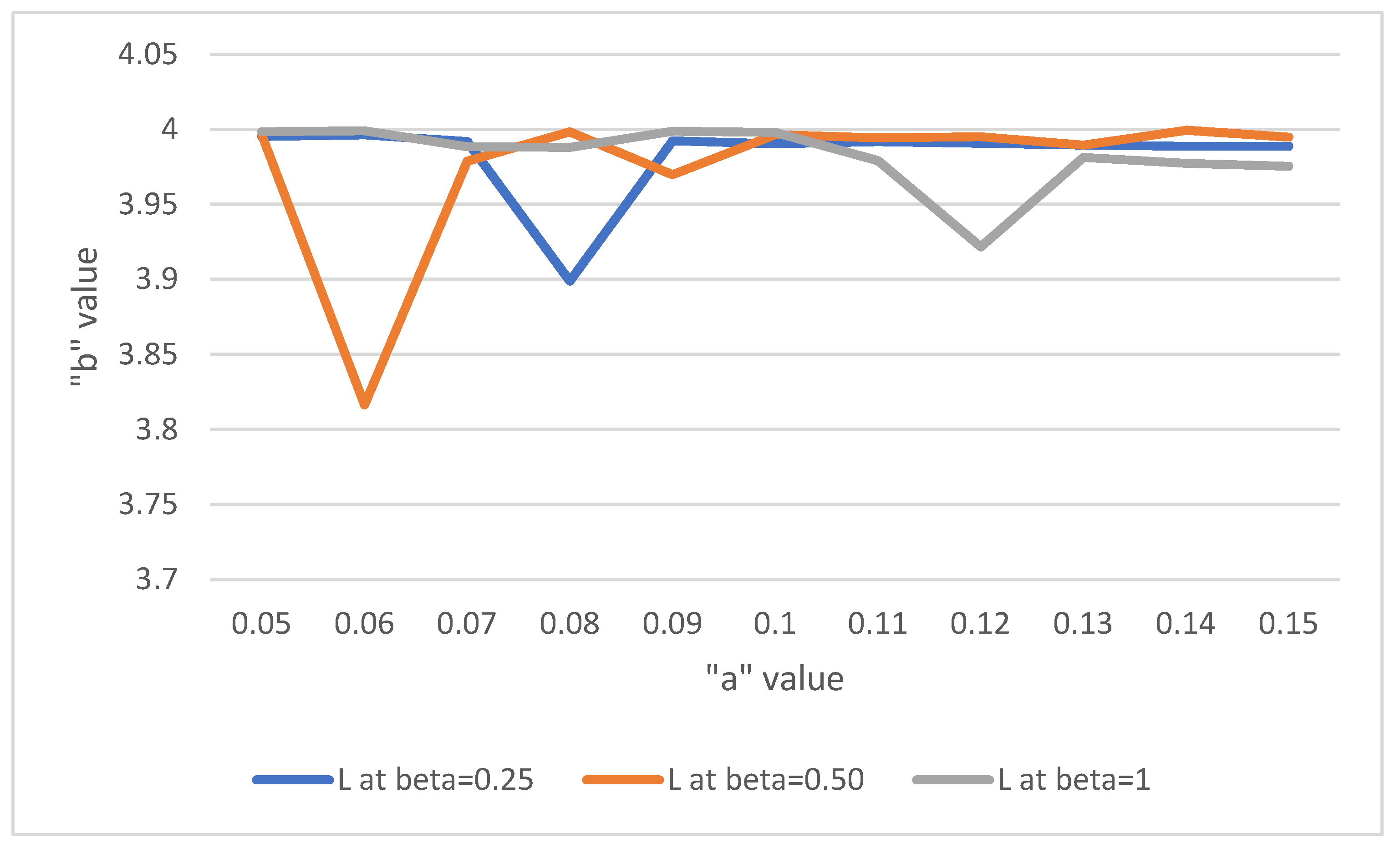
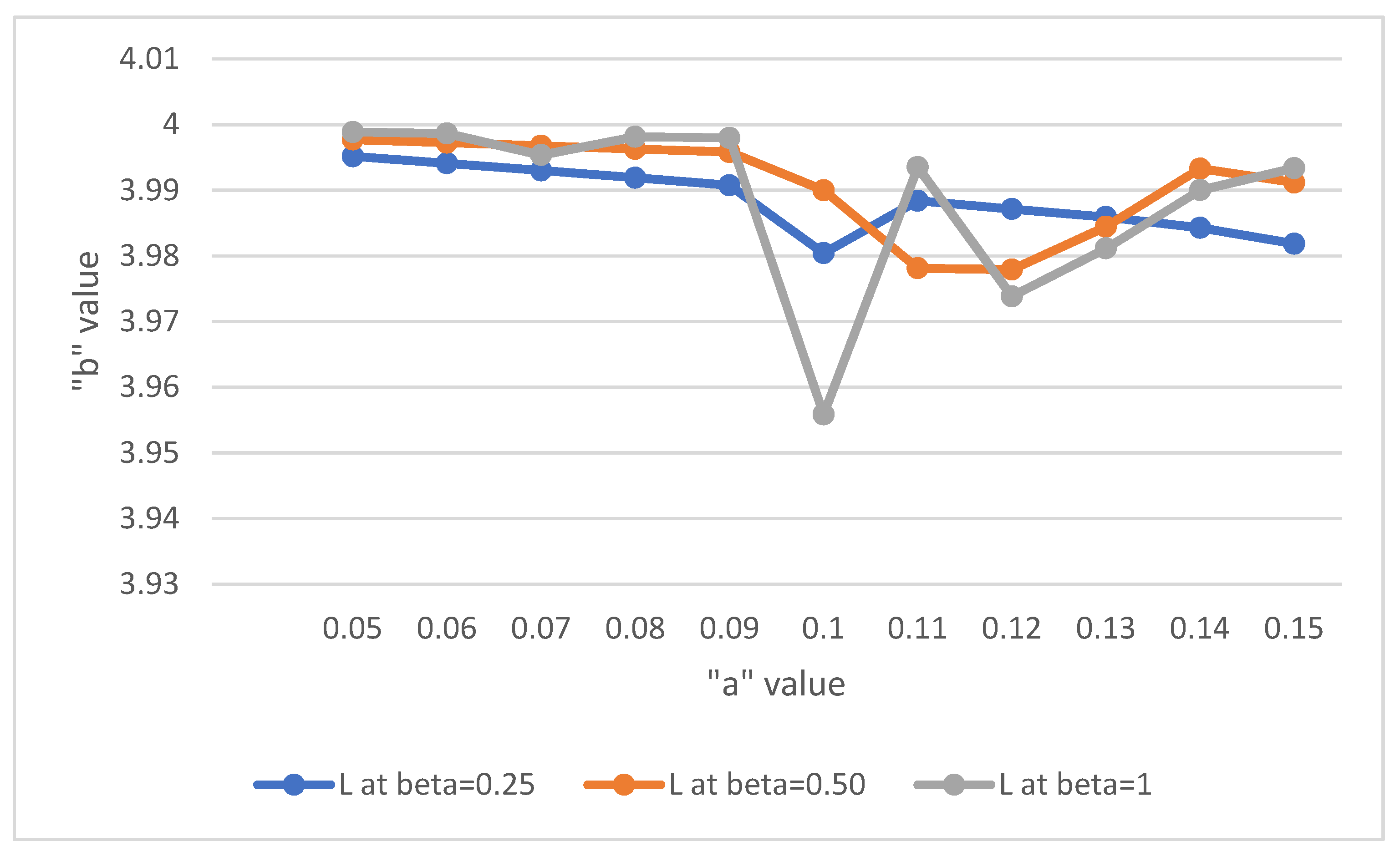
a	L at b = 0.25	L at b = 0.50	L at b = 1
0.05	3.995225	3.996138	3.998365
0.06	3.996334	3.816372	3.999065
0.07	3.991855	3.978771	3.988408
0.08	3.898826	3.998237	3.988041
0.09	3.992406	3.969705	3.998728
0.10	3.972794	3.996458	3.997931
0.11	3.991761	3.994401	3.979199
0.12	3.990751	3.995094	3.921691
0.13	3.989561	3.989560	3.981316
0.14	3.988700	3.999407	3.977291
0.15	3.988784	3.994852	3.975339

Table 2. Comparison of L-Expected number of units in the system between poisson and encouraged arrival.

a	Poisson Arrival L at b = 0.50	Encouraged Arrival L at b = 0.50
0.06	3.967179	3.816372

Table 3. Comparison of L-Expected number of units in the system between poisson and encouraged arrival.

a	Poisson Arrival L at b = 1	Encouraged Arrival L at b = 1
0.08	3.985963	3.988041
0.11	3.980742	3.979199
0.12	3.979004	3.921691

Table 4. Verification of Little’s law.

S.No	b	a	L	W	L/W	λ
1	0.25	0.05	3.995225	0.66587083	5.999998498	6
2	0.5	0.05	3.996334	0.66605567	5.999996997	6
3	1	0.05	3.998365	0.66639417	6.000001501	6
4	0.25	0.06	3.996334	0.66605567	5.999996997	6
5	0.5	0.06	3.816372	0.63606200	6	6
6	1	0.06	3.999065	0.66651083	5.9999985	6
7	0.25	0.07	3.991855	0.66531417	5.999956412	6
8	0.5	0.07	3.978771	0.66312850	5.999995476	6
9	1	0.07	3.988408	0.66473467	5.999996991	6
10	0.25	0.08	3.898826	0.64980433	6.000003078	6
11	0.5	0.08	3.998237	0.66637283	5.999998499	6
12	1	0.08	3.988041	0.66467350	5.999995487	6
13	0.25	0.09	3.992406	0.6654010	6	6
14	0.5	0.09	3.969705	0.6616175	5.999995466	6
15	1	0.09	3.998728	0.6664546	5.999996999	6
16	0.25	0.1	3.972794	0.6621323	6.000003021	6
17	0.5	0.1	3.996458	0.6660763	6.000003003	6
18	1	0.1	3.997931	0.6663218	5.999998499	6
19	0.25	0.11	3.991761	0.6652935	5.999995491	6
20	0.5	0.11	3.994401	0.6657335	5.999995494	6
21	1	0.11	3.979199	0.6631998	5.999998492	6
22	0.25	0.12	3.990751	0.6651251	6.000001503	6
23	0.5	0.12	3.995094	0.6658490	6	6
24	1	0.12	3.921691	0.6536151	6.00000153	6
25	0.25	0.13	3.989561	0.6649268	5.999998496	6
26	0.5	0.13	3.989560	0.6649266	5.999996992	6
27	1	0.13	3.981316	0.6635526	5.999996986	6
28	0.25	0.14	3.988700	0.6647833	6.000003009	6
29	0.5	0.14	3.999407	0.6665678	5.9999985	6
30	1	0.14	3.977291	0.6628818	5.999998491	6
31	0.25	0.15	3.988784	0.6647973	6.000030085	6
32	0.5	0.15	3.994852	0.6658086	5.999996996	6
33	1	0.15	3.975339	0.6625560	5.999995472	6

Solution of the system is determined by scheming L against “a” for some values of b, as given in Figure 1.

Figure 1. The relationship between L and “a” when “b” = 0.25, 0.50.

Remark 1.

From the Figure 1, it is evident that, the value of L-Expected number of units in the system is less at a = 0.06, 0.08, 0.12 comparing the poisson arrival.

The value of the parameters of this M/M/1/N queuing models are given.

λ	η	λ (1+η)	N	P	q	q	gi
4	0.6	6.4	4	0.1	0.9	0.25, 0.50, 1	0 or 1

The following Table 5, Table 6, Table 7 and Table 8 of values is obtained for L-expected number of units in the system by using the relation [11] for b = 0.25, 0.50, 1.

Table 5. The values of L for different values of b = 0.25, 0.50, 1.

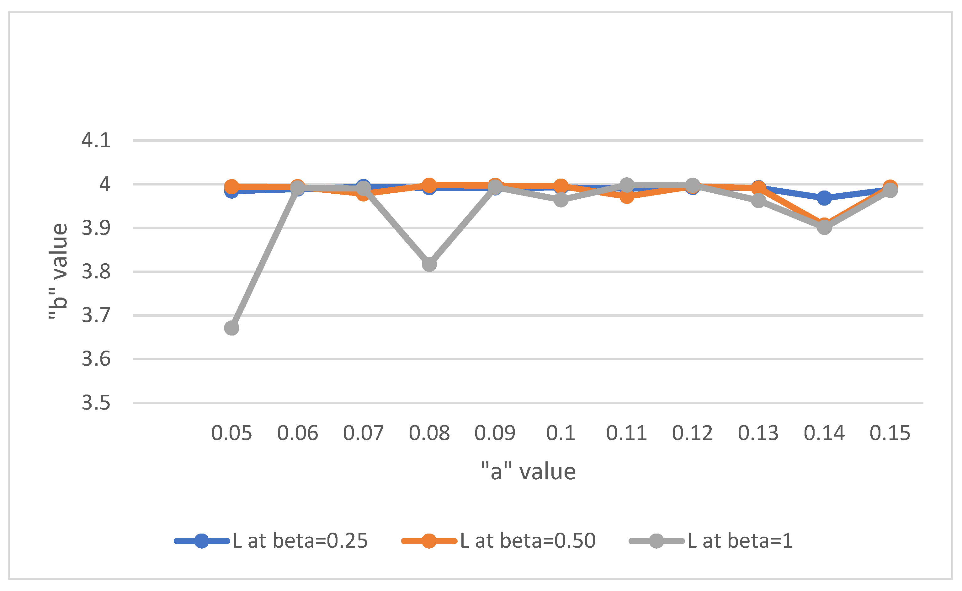
a	L at b = 0.25	L at b = 0.50	L at b = 1
0.05	3.984371	3.994342	3.670805
0.06	3.989045	3.994022	3.991227
0.07	3.994445	3.978169	3.990492
0.08	3.991879	3.997466	3.816650
0.09	3.991760	3.997145	3.993229
0.10	3.992748	3.995779	3.964409
0.11	3.990344	3.972103	3.998272
0.12	3.992591	3.995301	3.997578
0.13	3.992015	3.991104	3.962625
0.14	3.968499	3.906548	3.901016
0.15	3.988080	3.992987	3.985997

Table 6. Comparison of L-Expected number of units in the system between poisson and encouraged arrival.

a	Poisson Arrival L at b = 0.50	Encouraged Arrival L at b = 0.50
0.14	3.924853	3.906548

Table 7. Comparison of L-Expected number of units in the system between poisson and encouraged arrival.

a	Poisson Arrival L at b = 1	Encouraged Arrival L at b = 1
0.05	3.991214	3.670805
0.08	3.985968	3.816650
0.10	3.982482	3.964409
0.13	3.977268	3.962625
0.14	3.975535	3.901016

Table 8. Verification of Little’s law.

S.No	b	a	L	W	L/W	λ
1	0.25	0.05	3.984371	0.62255797	6.399999679	6.4
2	0.5	0.05	3.994342	0.62411594	6.399999359	6.4
3	1	0.05	3.670805	0.57356328	6.400003138	6.4
4	0.25	0.06	3.989045	0.62328828	6.400002888	6.4
5	0.5	0.06	3.994022	0.62406594	6.399999359	6.4
6	1	0.06	3.990492	0.62351438	6.400003849	6.4
7	0.25	0.07	3.994445	0.62413203	6.400008332	6.4
8	0.5	0.07	3.978169	0.62158891	6.399999035	6.4
9	1	0.07	3.990492	0.62351438	6.400003849	6.4
10	0.25	0.08	3.991879	0.62373109	6.400000962	6.4
11	0.5	0.08	3.997466	0.62460406	6.40000064	6.4
12	1	0.08	3.816650	0.59635156	6.399995305	6.4
13	0.25	0.09	3.991760	0.62371250	6.399994869	6.4
14	0.5	0.09	3.997145	0.62455391	6.399999039	6.4
15	1	0.09	3.993229	0.62394203	6.400000321	6.4
16	0.25	0.1	3.992748	0.62386688	6.399998718	6.4
17	0.5	0.1	3.995779	0.62434047	6.400004805	6.4
18	1	0.1	3.964409	0.61943891	6.399999031	6.4
19	0.25	0.11	3.990344	0.62349125	6.400002566	6.4
20	0.5	0.11	3.972103	0.62064109	6.400000967	6.4
21	1	0.11	3.998272	0.62473000	6.4	6.4
22	0.25	0.12	3.992591	0.62384234	6.400003527	6.4
23	0.5	0.12	3.995301	0.62426578	6.399997757	6.4
24	1	0.12	3.997578	0.62466844	6.399524227	6.4
25	0.25	0.13	3.992015	0.62375234	6.400003527	6.4
26	0.5	0.13	3.991104	0.62361000	6.4	6.4
27	1	0.13	3.962625	0.61916016	6.400001615	6.4
28	0.25	0.14	3.968499	0.62007797	6.399999677	6.4
29	0.5	0.14	3.906548	0.61039813	6.400001311	6.4
30	1	0.14	3.901016	0.60953375	6.399997375	6.4
31	0.25	0.15	3.988080	0.6231375	6.399994865	6.4
32	0.5	0.15	3.992987	0.62390422	6.400002244	6.4
33	1	0.15	3.985997	0.62281203	6.400000321	6.4

Solution of the system is determined by scheming L against “a” for some values of b, as given in Figure 2.

Figure 2. The relationship between L and “a” when “b” = 0.25, 0.50, 1.

Remark 2.

From the Figure 2, it is evident that, the value of L-Expected number of units in the system is less at a = 0.05, 0.08, 0.14 comparing the poisson arrival.

The value of the parameters of this M/M/1/N queuing models are given.

λ	η	λ (1+η)	N	P	q	q	gi
4	0.7	6.8	4	0.1	0.9	0.25, 0.50, 1	0 or 1

The following Table 9, Table 10, Table 11 and Table 12 of values is obtained for L-expected number of units in the system by using the relation [11] for b = 0.25, 0.50, 1.

Table 9. The values of L for different values of b = 0.25, 0.50, 1.

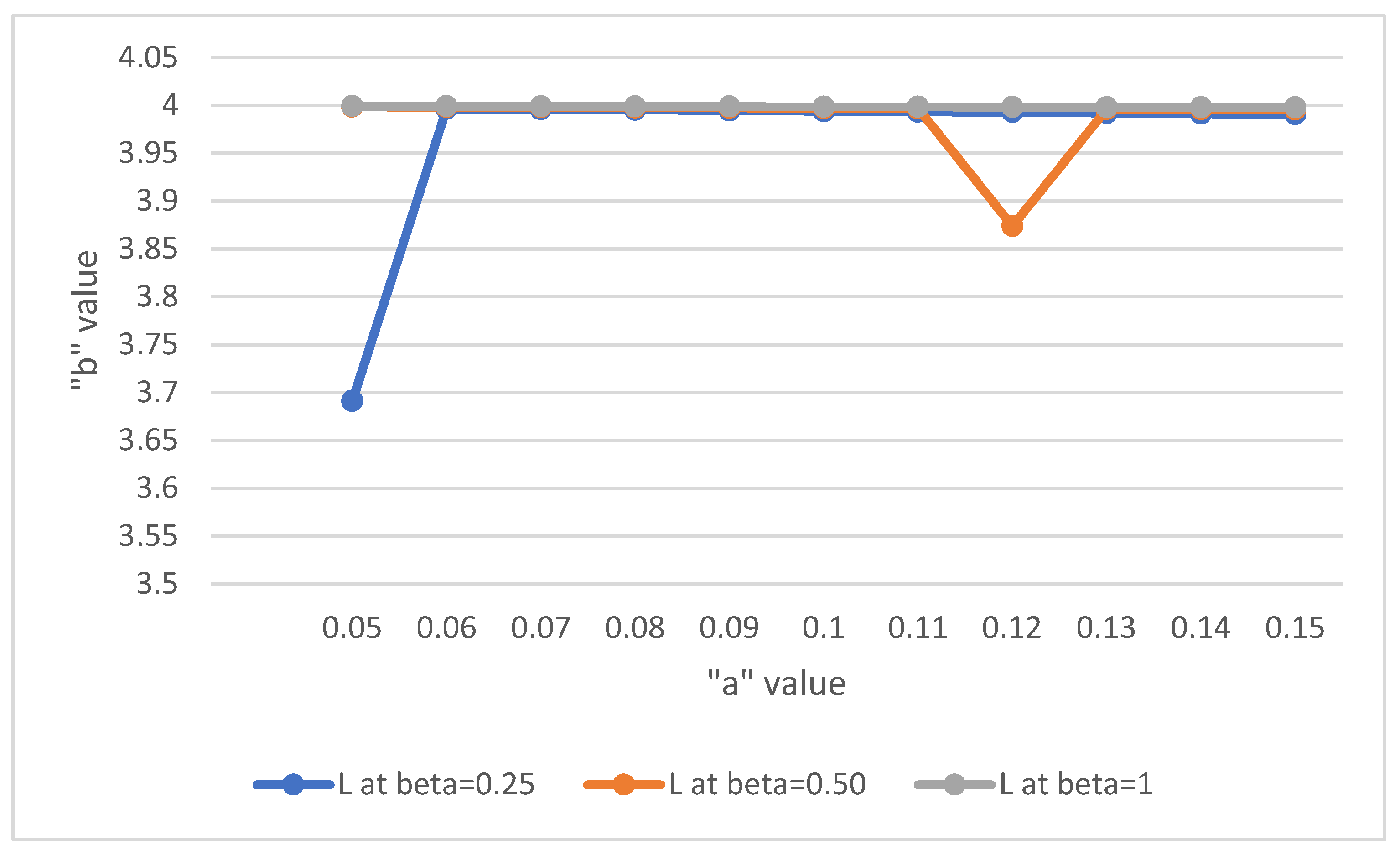
a	L at b = 0.25	L at b = 0.50	L at b = 1
0.05	3.691028	3.998519	3.999239
0.06	3.996364	3.998222	3.999115
0.07	3.995741	3.997918	3.998966
0.08	3.995176	3.997620	3.998820
0.09	3.994538	3.997342	3.998671
0.10	3.993821	3.997006	3.998423
0.11	3.993171	3.996615	3.998422
0.12	3.992940	3.873728	3.998231
0.13	3.991847	3.996127	3.998082
0.14	3.991183	3.995767	3.997902
0.15	3.990506	3.995525	3.997780

Table 10. Comparison of L-Expected number of units in the system between poisson and encouraged arrival.

a	Poisson Arrival L at b = 0.50	Encouraged Arrival L at b = 0.50
0.05	3.908215	3.691028

Table 11. Comparison of L-Expected number of units in the system between poisson and encouraged arrival.

a	Poisson Arrival L at b = 1	Encouraged Arrival L at b = 1
0.12	3.935285	3.873728

Table 12. Verification of Little’s law.

S.No	B	a	L	W	L/W	λ
1	0.25	0.05	3.691028	0.54279824	6.800002948	6.8
2	0.5	0.05	3.998519	0.58801750	6.799994218	6.8
3	1	0.05	3.999239	0.58812338	6.800004421	6.8
4	0.25	0.06	3.996364	0.58770059	6.799995236	6.8
5	0.5	0.06	3.998222	0.58797382	6.799997959	6.8
6	1	0.06	3.999115	0.58810515	6.8000017	6.8
7	0.25	0.07	3.995741	0.58760897	6.79999966	6.8
8	0.5	0.07	3.997918	0.58792912	6.800001361	6.8
9	1	0.07	3.998966	0.58808324	6.800002721	6.8
10	0.25	0.08	3.995176	0.58752588	6.799998638	6.8
11	0.5	0.08	3.997620	0.58788529	6.800003402	6.8
12	1	0.08	3.998820	0.58806176	6.799997279	6.8
13	0.25	0.09	3.994538	0.58743206	6.800000681	6.8
14	0.5	0.09	3.997342	0.58784441	6.800004763	6.8
15	1	0.09	3.998671	0.58803985	6.799998299	6.8
16	0.25	0.1	3.993821	0.58732662	6.799995573	6.8
17	0.5	0.1	3.997006	0.58779500	6.8	6.8
18	1	0.1	3.998423	0.58800338	6.800004422	6.8
19	0.25	0.11	3.993171	0.58723103	6.800000341	6.8
20	0.5	0.11	3.996615	0.58773750	6.799994215	6.8
21	1	0.11	3.998422	0.58800324	6.800002721	6.8
22	0.25	0.12	3.992940	0.58719706	6.800000681	6.8
23	0.5	0.12	3.873728	0.56966588	6.799998596	6.8
24	1	0.12	3.998231	0.58797515	6.800001701	6.8
25	0.25	0.13	3.991847	0.58703632	6.800003748	6.8
26	0.5	0.13	3.996127	0.58766574	6.799996937	6.8
27	1	0.13	3.998082	0.58795324	6.800002721	6.8
28	0.25	0.14	3.991183	0.58693868	6.799996252	6.8
29	0.5	0.14	3.995767	0.58761279	6.799997617	6.8
30	1	0.14	3.997902	0.58792676	6.799997279	6.8
31	0.25	0.15	3.990506	0.58683912	6.800001363	6.8
32	0.5	0.15	3.995525	0.58757721	6.800002383	6.8
33	1	0.15	3.997780	0.58790882	6.799997959	6.8

Solution of the system is determined by scheming L against “a” for some values of b, as given in Figure 3.

Figure 3. The relationship between L and “a” when “b” = 0.25, 0.50, 1.

Remark 3.

From the Figure 3, it is evident that, the value of L-Expected number of units in the system is less at a = 0.05, 0.12 comparing the poisson arrival.

The value of the parameters of this M/M/1/N queuing models are given.

λ	η	λ (1+η)	N	P	q	q	gi
4	0.8	7.2	4	0.1	0.9	0.25, 0.50, 1	0 or 1

The following Table 13, Table 14, Table 15 and Table 16 of values is obtained for L-expected number of units in the system by using the relation [11] for b = 0.25, 0.50, 1.

Table 13. The values of L for different values of b = 0.25, 0.50, 1.

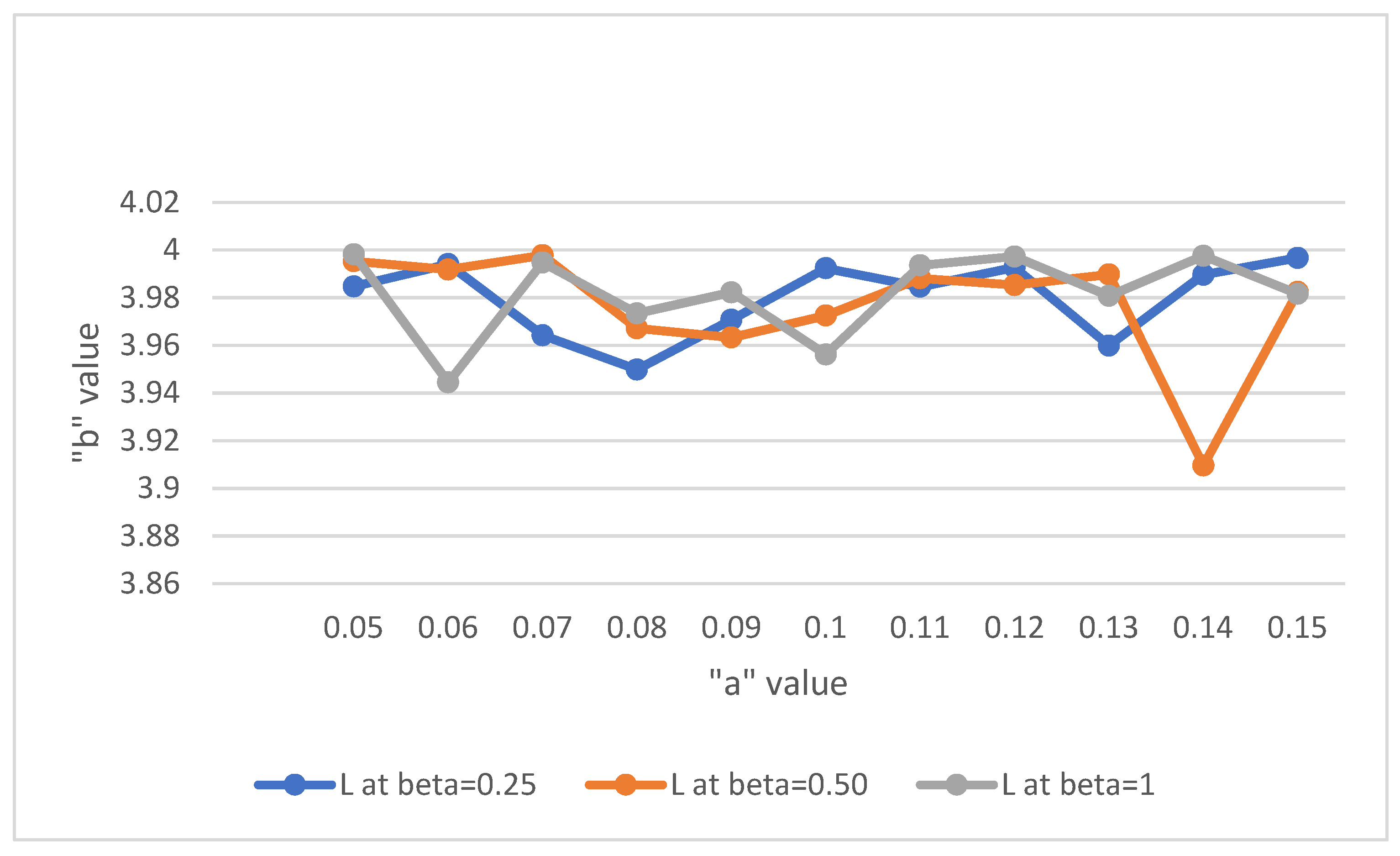
a	L at b = 0.25	L at b = 0.50	L at b = 1
0.05	3.984716	3.995301	3.998185
0.06	3.994041	3.991779	3.944412
0.07	3.964199	3.997761	3.994704
0.08	3.949832	3.967141	3.973384
0.09	3.970734	3.963279	3.982187
0.10	3.992297	3.972509	3.956158
0.11	3.984562	3.988086	3.993573
0.12	3.992639	3.985290	3.997242
0.13	3.959906	3.989724	3.980712
0.14	3.989582	3.909560	3.997553
0.15	3.996673	3.982409	3.981590

Table 14. Comparison of L-Expected number of units in the system between poisson and encouraged arrival.

a	Poisson Arrival L at b = 0.50	Encouraged Arrival L at b = 0.50
0.14	3.924853	3.909560

Table 15. Comparison of L-Expected number of units in the system between poisson and encouraged arrival.

a	Poisson Arrival L at b = 1	Encouraged Arrival L at b = 1
0.06	3.989463	3.944412
0.08	3.985968	3.973384
0.09	3.984224	3.982187
0.10	3.982482	3.956158

Table 16. Verification of Little’s law.

S.No	b	a	L	W	L/W	λ
1	0.25	0.05	3.984716	0.55343278	7.199997109	7.2
2	0.5	0.05	3.995301	0.55490292	7.199998919	7.2
3	1	0.05	3.998185	0.55530347	7.200006123	7.2
4	0.25	0.06	3.994041	0.55472792	7.199998918	7.2
5	0.5	0.06	3.991779	0.55441375	7.199996753	7.2
6	1	0.06	3.944412	0.54783500	7.2	7.2
7	0.25	0.07	3.964199	0.55058319	7.200002543	7.2
8	0.5	0.07	3.997761	0.55524458	7.199994597	7.2
9	1	0.07	3.994704	0.55482000	7.2	7.2
10	0.25	0.08	3.949832	0.54858778	7.199997083	7.2
11	0.5	0.08	3.967141	0.55099181	7.199997459	7.2
12	1	0.08	3.973384	0.55185889	7.19999855	7.2
13	0.25	0.09	3.970734	0.55149083	7.199997824	7.2
14	0.5	0.09	3.963279	0.55045542	7.20000545	7.2
15	1	0.09	3.982187	0.55308153	7.199993853	7.2
16	0.25	0.1	3.992297	0.55448569	7.199996032	7.2
17	0.5	0.1	3.972509	0.55173736	7.200004712	7.2
18	1	0.1	3.956158	0.54946639	7.200005096	7.2
19	0.25	0.11	3.984562	0.55341139	7.20000506	7.2
20	0.5	0.11	3.988086	0.55390083	7.199997834	7.2
21	1	0.11	3.993573	0.55466292	7.199998918	7.2
22	0.25	0.12	3.992639	0.55453319	7.200002525	7.2
23	0.5	0.12	3.985290	0.55351250	7.199993496	7.2
24	1	0.12	3.997242	0.55517250	7.199993516	7.2
25	0.25	0.13	3.959906	0.54998694	7.199999273	7.2
26	0.5	0.13	3.989724	0.55412833	7.200004331	7.2
27	1	0.13	3.980712	0.55287667	7.199995659	7.2
28	0.25	0.14	3.989582	0.55410861	7.199994947	7.2
29	0.5	0.14	3.909560	0.54299444	7.200005893	7.2
30	1	0.14	3.997553	0.55521569	7.199996038	7.2
31	0.25	0.15	3.996673	0.55509347	7.200006125	7.2
32	0.5	0.15	3.982409	0.55311236	7.200004701	7.2
33	1	0.15	3.981590	0.55299861	7.199994937	7.2

The solution of the system is determined by scheming L against “a” for some values of b, as given in Figure 4.

Figure 4. The relationship between L and “a” when “b” = 0.25, 0.50, 1.

Remark 4.

From the Figure 4, it is evident that, the value of L-Expected number of units in the system is less at a = 0.06, 0.08, 0.09, 0.10, 0.12, 0.13, 0.14 comparing the poisson arrival.

The value of the parameters of this M/M/1/N queuing models are given.

λ	η	λ (1+η)	N	P	q	q	gi
4	0.9	7.6	4	0.1	0.9	0.25, 0.50, 1	0 or 1

The following Table 17, Table 18, Table 19, Table 20 and Table 21 of values is obtained for L-expected number of units in the system by using the relation [11] for b = 0.25, 0.50, 1.

Table 17. The values of L for different values of b = 0.25, 0.50, 1.

a	L at b = 0.25	L at b = 0.50	L at b = 1
0.05	3.80713	3.95550	3.89270
0.06	3.96457	3.80124	3.37690
0.07	3.88220	3.87680	3.71920
0.08	3.71410	3.97520	3.98390
0.09	3.98960	3.93560	3.96960
0.10	3.80066	3.94490	3.63780
0.11	3.83620	3.75970	3.95590
0.12	3.98890	3.94710	3.99470
0.13	3.98770	3.99320	3.97470
0.14	3.98853	3.97796	3.98021
0.15	3.96290	3.69889	3.97548

Table 18. Comparison of L-Expected number of units in the system between poisson and encouraged arrival.

a	Poisson Arrival L at b = 0.25	Encouraged Arrival L at b = 0.25
0.05	3.908215	3.80713
0.08	3.856900	3.71410
0.10	3.824116	3.80066

Table 19. Comparison of L-Expected number of units in the system between poisson and encouraged arrival.

a	Poisson Arrival L at b = 0.50	Encouraged Arrival L at b = 0.50
0.05	3.972583	3.95550
0.06	3.967179	3.80124
0.07	3.961800	3.87680
0.09	3.951119	3.93560
0.10	3.945816	3.94490
0.11	3.940538	3.75970
0.15	3.919673	3.69889

Table 20. Comparison of L-Expected number of units in the system between poisson and encouraged arrival.

a	Poisson Arrival L at b = 1	Encouraged Arrival L at b = 1
0.05	3.9912	3.8927
0.06	3.9894	3.3769
0.07	3.9877	3.7192
0.08	3.9859	3.9839
0.09	3.9842	3.9696
0.10	3.9824	3.6378
0.11	3.9807	3.9559
0.13	3.9772	3.9747

Table 21. Verification of Little’s law.

S.No	b	a	L	W	L/W	λ
1	0.25	0.05	3.80713	0.50093816	7.600002396	7.6
2	0.5	0.05	3.95550	0.52046053	7.599993083	7.6
3	1	0.05	3.89270	0.51219737	7.600109334	7.6
4	0.25	0.06	3.96457	0.52165395	7.599999233	7.6
5	0.5	0.06	3.80124	0.50016316	7.600002399	7.6
6	1	0.06	3.37690	0.44432895	7.599999100	7.6
7	0.25	0.07	3.88220	0.51081579	7.599996868	7.6
8	0.5	0.07	3.87680	0.51010526	7.600003921	7.6
9	1	0.07	3.71920	0.48936842	7.600006539	7.6
10	0.25	0.08	3.71410	0.48869737	7.600005730	7.6
11	0.5	0.08	3.97520	0.52305263	7.599994647	7.6
12	1	0.08	3.98390	0.52419737	7.600005342	7.6
13	0.25	0.09	3.98960	0.52494737	7.600005334	7.6
14	0.5	0.09	3.93560	0.51784211	7.600001545	7.6
15	1	0.09	3.96960	0.52231579	7.599996937	7.6
16	0.25	0.1	3.80066	0.50008684	7.599997600	7.6
17	0.5	0.1	3.94490	0.51906579	7.599996918	7.6
18	1	0.1	3.63780	0.47865789	7.599998329	7.6
19	0.25	0.11	3.83620	0.50476316	7.600002377	7.6
20	0.5	0.11	3.75970	0.49469737	7.60000566	7.6
21	1	0.11	3.95590	0.52051316	7.600002305	7.6
22	0.25	0.12	3.98890	0.52485526	7.600003811	7.6
23	0.5	0.12	3.94710	0.51935526	7.600003851	7.6
24	1	0.12	3.99470	0.52561842	7.600006088	7.6
25	0.25	0.13	3.98770	0.52469737	7.600005336	7.6
26	0.5	0.13	3.99320	0.52542105	7.600000761	7.6
27	1	0.13	3.97470	0.52298684	7.599997705	7.6
28	0.25	0.14	3.98853	0.52480658	7.599993903	7.6
29	0.5	0.14	3.97796	0.52341579	7.599996943	7.6
30	1	0.14	3.98021	0.52371184	7.599997709	7.6
31	0.25	0.15	3.96290	0.52143526	7.600003836	7.6
32	0.5	0.15	3.69889	0.48669605	7.600000822	7.6
33	1	0.15	3.97548	0.52308947	7.600006882	7.6

The solution of the system is determined by scheming L against a for some values of b, as given in Figure 5.

Figure 5. The relationship between L and “a” when “b” = 0.25, 0.50, 1.

Remark 5.

From the Figure 5, it is evident that, the value of L-Expected number of units in the system is less at a = 0.06, 0.08, 0.09, 0.10, 0.11, 0.12, 0.14, 0.15 comparing the poisson arrival.

The value of the parameters of this M/M/1/N queuing models are given below.

λ	η	λ (1+η)	N	P	q	q	gi
4	0.11	4.44	4	0.1	0.9	0.25, 0.50, 1	0 or 1

The following Table 22, Table 23, Table 24, Table 25 and Table 26 of values is obtained for L-expected number of units in the system by using the relation [11] for b = 0.25, 0.50, 1.

Table 22. The values of L for different values of b = 0.25, 0.50, 1.

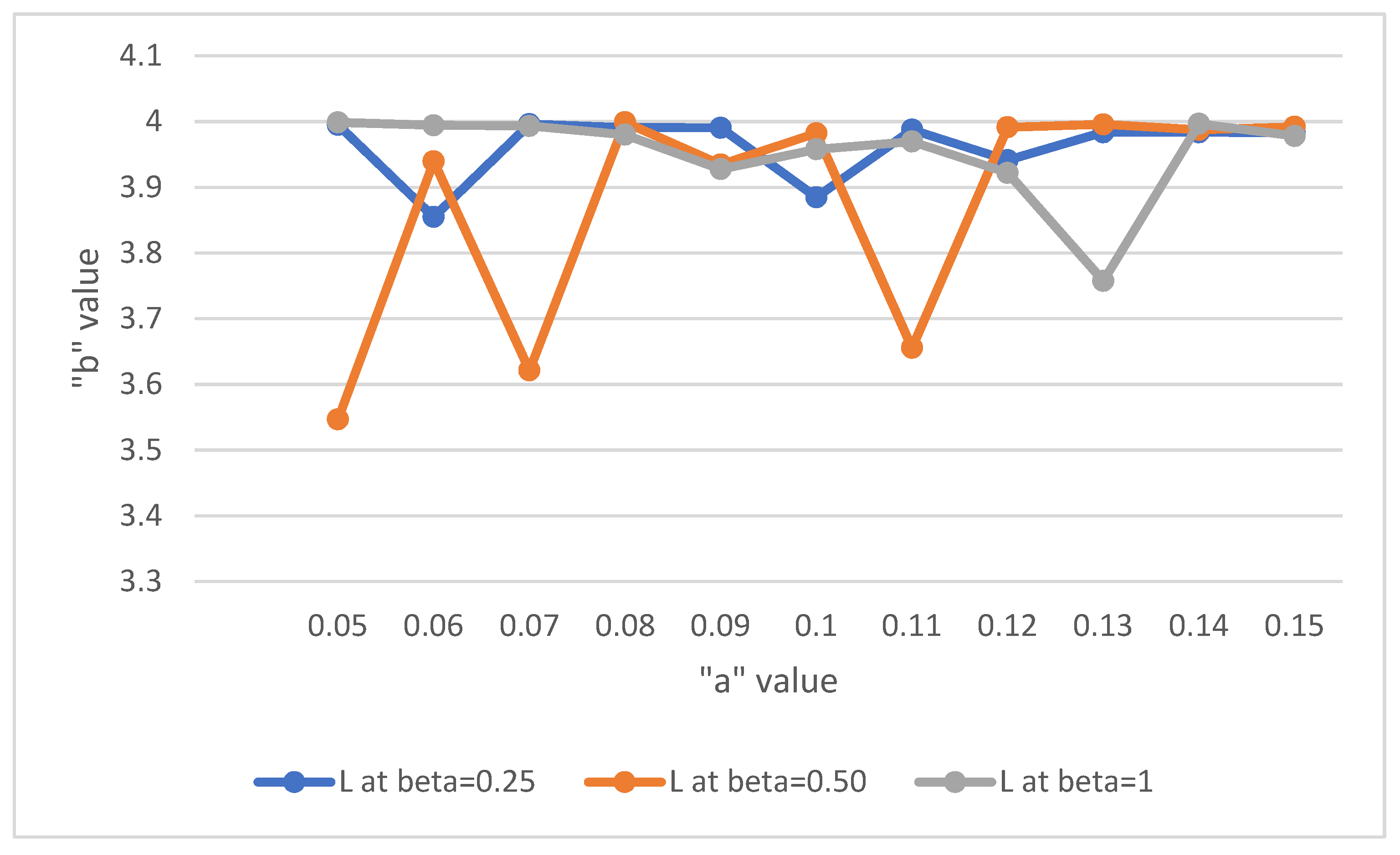
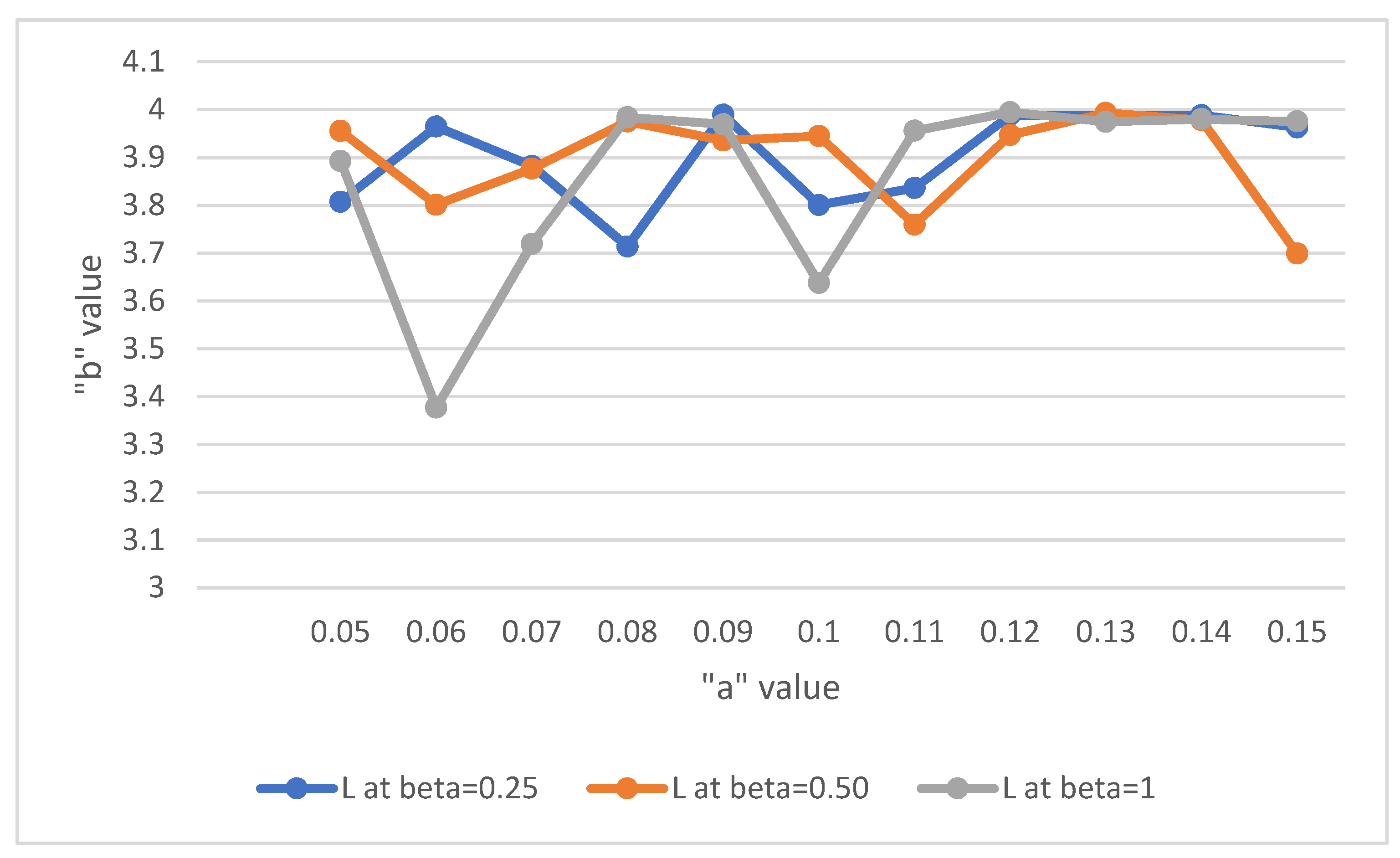
a	L at b = 0.25	L at b = 0.50	L at b = 1
0.05	3.995100	3.546800	3.998800
0.06	3.854856	3.939360	3.994395
0.07	3.996000	3.621280	3.993300
0.08	3.991044	3.999263	3.980034
0.09	3.990490	3.934637	3.927608
0.10	3.884795	3.982260	3.957856
0.11	3.987600	3.655474	3.969599
0.12	3.941250	3.991380	3.922006
0.13	3.983723	3.995832	3.757424
0.14	3.983723	3.987378	3.996665
0.15	3.983001	3.992066	3.978019

Table 23. Comparison of L-Expected number of units in the system between poisson and encouraged arrival.

a	Poisson Arrival L at b = 0.25	Encouraged Arrival L at b = 0.25
0.06	3.890814	3.854856

Table 24. Comparison of L-Expected number of units in the system between poisson and encouraged arrival.

a	Poisson Arrival L at b = 0.50	Encouraged Arrival L at b = 0.50
0.05	3.97258	3.54680
0.06	3.96717	3.93936
0.07	3.96180	3.62128
0.09	3.95111	3.93463
0.11	3.94053	3.65547

Table 25. Comparison of L-Expected number of units in the system between poisson and encouraged arrival.

a	Poisson Arrival L at b = 1	Encouraged Arrival L at b = 1
0.08	3.98596	3.980034
0.09	3.98422	3.927608
0.10	3.98248	3.957856
0.11	3.98074	3.969599
0.13	3.97726	3.757424

Table 26. Verification of Little’s law.

S.No	b	a	L	W	L/W	λ
1	0.25	0.05	3.9951	0.8997973	4.440001467	4.44
2	0.5	0.05	3.5468	0.79882883	4.439999049	4.44
3	1	0.05	3.9988	0.90063063	4.439998179	4.44
4	0.25	0.06	3.854856	0.86821081	4.439999032	4.44
5	0.5	0.06	3.93936	0.88724324	4.440001217	4.44
6	1	0.06	3.9943953	0.89963858	4.439997933	4.44
7	0.25	0.07	3.996	0.9	4.44	4.44
8	0.5	0.07	3.62128	0.8156036	4.439997842	4.44
9	1	0.07	3.9933	0.89939189	4.439999466	4.44
10	0.25	0.08	3.991044	0.89888378	4.439998932	4.44
11	0.5	0.08	3.999263	0.90073491	4.439999556	4.44
12	1	0.08	3.980034	0.89640405	4.440000268	4.44
13	0.25	0.09	3.99049	0.89875901	4.440000045	4.44
14	0.5	0.09	3.934637	0.8861795	4.439997517	4.44
15	1	0.09	3.927608	0.8845964	4.44000199	4.44
16	0.25	0.1	3.884795	0.87495383	4.439999131	4.44
17	0.5	0.1	3.98226	0.89690541	4.440002007	4.44
18	1	0.1	3.957856	0.89140901	4.440000045	4.44
19	0.25	0.11	3.9876	0.89810811	4.440000534	4.44
20	0.5	0.11	3.655474	0.82330495	4.439999757	4.44
21	1	0.11	3.969599	0.89405383	4.43999915	4.44
22	0.25	0.12	3.94125	0.88766892	4.439999594	4.44
23	0.5	0.12	3.99138	0.89895946	4.440002269	4.44
24	1	0.12	3.922006	0.88333468	4.439998415	4.44
25	0.25	0.13	3.983723	0.89723491	4.439999554	4.44
26	0.5	0.13	3.995832	0.89996216	4.4400008	4.44
27	1	0.13	3.757424	0.84626667	4.439998251	4.44
28	0.25	0.14	3.983723	0.89723491	4.439999554	4.44
29	0.5	0.14	3.987378	0.89805811	4.440000534	4.44
30	1	0.14	3.996665	0.90014977	4.439998889	4.44
31	0.25	0.15	3.9830014	0.89707239	4.440001917	4.44
32	0.5	0.15	3.992066	0.89911396	4.439999822	4.44
33	1	0.15	3.978019	0.89595023	4.440001116	4.44

The solution of the system is determined by scheming L against a for some values of b, as given in Figure 6.

Figure 6. The relationship between L and “a” when “b” = 0.25, 0.50, 1.

Remark 6.

From the Figure 6, it is evident that, the value of L-Expected number of units in the system is less at a = 0.05, 0.06, 0.07, 0.11, 0.13, comparing the poisson arrival.

The value of the parameters of this M/M/1/N queuing models are given.

λ	η	λ (1+η)	N	P	q	q	gi
4	0.12	4.48	4	0.1	0.9	0.25, 0.50, 1	0 or 1

The following Table 27, Table 28 and Table 29 of values is obtained for L-expected number of units in the system by using the relation [11] for b = 0.25, 0.50, 1.

Table 27. The values of L for different values of b = 0.25, 0.50, 1.

a	L at b = 0.25	L at b = 0.50	L at b = 1
0.05	3.995172	3.997721	3.998884
0.06	3.994119	3.997247	3.998651
0.07	3.993030	3.996783	3.995359
0.08	3.991918	3.996305	3.998160
0.09	3.990777	3.995824	3.997972
0.10	3.980430	3.990005	3.955846
0.11	3.988407	3.978139	3.993533
0.12	3.987155	3.977938	3.973857
0.13	3.985937	3.984462	3.981141
0.14	3.984280	3.993300	3.990031
0.15	3.981860	3.991190	3.993370

Table 28. Comparison of L-Expected number of units in the system between poisson and encouraged arrival.

a	Poisson Arrival L at b = 1	Encouraged Arrival L at b = 1
0.10	3.98248	3.955846

Table 29. Verification of Little’s law.

S.No	b	a	L	W	L/W	λ
1	0.25	0.05	3.995172	0.89177946	4.480002332	4.48
2	0.5	0.05	3.997721	0.89234844	4.480002196	4.48
3	1	0.05	3.998884	0.89260804	4.480000179	4.48
4	0.25	0.06	3.994119	0.89154442	4.480002109	4.48
5	0.5	0.06	3.997247	0.89224263	4.479998162	4.48
6	1	0.06	3.998651	0.89255603	4.480000134	4.48
7	0.25	0.07	3.99303	0.89130134	4.480001705	4.48
8	0.5	0.07	3.996783	0.89213906	4.480000314	4.48
9	1	0.07	3.995359	0.89182121	4.480001032	4.48
10	0.25	0.08	3.991918	0.89105313	4.480000628	4.48
11	0.5	0.08	3.996305	0.89203237	4.480001838	4.48
12	1	0.08	3.99816	0.89244643	4.480002151	4.48
13	0.25	0.09	3.990777	0.89079844	4.4800022	4.48
14	0.5	0.09	3.995824	0.8919317	4.47996484	4.48
15	1	0.09	3.997972	0.89240446	4.480002331	4.48
16	0.25	0.1	3.98043	0.88848884	4.47999919	4.48
17	0.5	0.1	3.990005	0.89062612	4.480000584	4.48
18	1	0.1	3.955846	0.88300134	4.480001721	4.48
19	0.25	0.11	3.988407	0.89026942	4.480002112	4.48
20	0.5	0.11	3.978139	0.88797746	4.480002297	4.48
21	1	0.11	3.993533	0.89141362	4.47999807	4.48
22	0.25	0.12	3.987155	0.88998996	4.479999775	4.48
23	0.5	0.12	3.977938	0.88793259	4.479997928	4.48
24	1	0.12	3.973857	0.88702165	4.479998241	4.48
25	0.25	0.13	3.985937	0.88971808	4.480000405	4.48
26	0.5	0.13	3.9844625	0.88938895	4.479999753	4.48
27	1	0.13	3.981141	0.88864754	4.479997704	4.48
28	0.25	0.14	3.98428	0.88934821	4.480001079	4.48
29	0.5	0.14	3.9933	0.89136161	4.479998025	4.48
30	1	0.14	3.990031	0.89063192	4.479999596	4.48
31	0.25	0.15	3.98186	0.88880804	4.48000018	4.48
32	0.5	0.15	3.99119	0.89089063	4.479998114	4.48
33	1	0.15	3.99337	0.89137723	4.480001167	4.48

The solution of the system is determined by scheming L against “a” for some values of b, as given in Figure 7.

Figure 7. The relationship between L and “a” when “b” = 0.25, 0.50, 1.

Remark 7.

From the Figure 5, it is evident that, the value of L-Expected number of units in the system is less at a = 0.10, 0.11, 0.12 comparing the poisson arrival.

5. Main Result and Discussion

When compared to Poisson arrival, encouraged arrival is more effective in handling service without delays. The (Table 1, Table 2, Table 3, Table 4, Table 5, Table 6, Table 7, Table 8, Table 9, Table 10, Table 11, Table 12, Table 13, Table 14, Table 15, Table 16, Table 22, Table 23, Table 24, Table 25, Table 26, Table 27, Table 28 and Table 29) shows that L-Expected number of units in the system is lower for the model prescribed here on comparing with the Poisson arrival model. It is also found that the Table 17, Table 18, Table 19 and Table 20 shows that adopting encouraged arrivals as well as increasing discounts in place of the model with Poisson arrival, greatly reduces W—the expected waiting time in the system.

Limitations

• This concept only suitable for M/M/1/N and M/M/1/K Queuing model;
• This concept will reduce the waiting time of customers for M/M/1/N Queuing model;
• This concept is valid for all real life applications with single service mechanism;
• The real life applications are always with finite capacity.

6. Conclusions

The encouraged arrival is quite valuable for many different businesses in terms of managing operations, deliberating, outlining, implementation, service development, and so on for consumers. In this study, we explored feedback, balking, retaining reneged clients and the quality control technique impact the encouraged arrival queuing model. The steady state scenario and iterative technique approach were utilized to create an analytical solution for the feedback M/M/1/N model’s quality control. From to (Table 1, Table 2, Table 3, Table 4, Table 5, Table 6, Table 7, Table 8, Table 9, Table 10, Table 11, Table 12, Table 13, Table 14, Table 15, Table 16, Table 22, Table 23, Table 24, Table 25, Table 26, Table 27, Table 28 and Table 29), the system’s waiting time is much decreased by adopting the encouraged arrivals and increasing discounts supplied instead of Poisson arrivals. Table 17, Table 18, Table 19 and Table 20 also shows that the waiting time is minimized to the greatest degree possible.

References

- Haight, F.A. Queuing with balking, I. Biometrika 1960, 47, 285–296. [Google Scholar] [CrossRef]
- Haight, F.A. Queueing with Reneging. Metrika 1959, 2, 186–197. [Google Scholar] [CrossRef]
- Ancker, C.J., Jr.; Gafarian, A.V. Some queuing problems with balking and reneging I. Oper. Res. 1963, 11, 88–100. [Google Scholar] [CrossRef]
- Ancker, C.J., Jr.; Gafarian, A.V. Some queuing problems with balking and reneging II. Oper. Res. 1963, 11, 928–937. [Google Scholar] [CrossRef]
- Hsu, L.; Tapiero, C.S. An economic model for determining the optimal quality and process control policy in a queue-like production system. Int. J. Prod. Res. 1990, 28, 1447–1457. [Google Scholar] [CrossRef]
- Abou-El-Ata, M.O. The State-Dependent Queue: M/M/1/N with Reneging and General Balk Functions. Microelectron. Reliab. 1991, 31, 1001–1007. [Google Scholar] [CrossRef]
- Hsu, L.; Tapiero, C.S. Integration of process monitoring, quality control and maintenance in an M/G/1 queue-like production system. Int. J. Prod. Res. 1992, 30, 2363–2379. [Google Scholar] [CrossRef]
- Fan-Orzechowski, X.; Feinberg, E.A. Optimal Admission Control for a Markovian Queue under the Quality of Service Constraint. In Proceedings of the 44th IEEE Conference on Decision and Control and the European Control Conference, Seville, Spain, 12–15 December 2005; pp. 1729–1734. [Google Scholar]
- Kumar, R.; Sharma, S.K. M/M/1/N Queuing System with Retention of Reneged Customers. Pak. J. Stat. Oper. Res. 2012, 8, 859–866. [Google Scholar] [CrossRef] [Green Version]
- Kumar, R.; Sharma, S.K. An M/M/1/N Queuing Model with Retention of reneged customers and Balking. Am. J. Oper. Res. 2012, 2, 1–5. [Google Scholar]
- Sharma, S.K.; Kumar, R. A Markovian Feedback Queue with Retention of Reneged Customers. Adv. Model. Optim. 2012, 14, 681–688. [Google Scholar]
- Jain, N.K.; Kumar, R.; Som, B.K. An M/M/1/N Queuing system with reverse balking. Am. J. Oper. Res. 2014, 4, 17–20. [Google Scholar]
- Som, B.K.; Seth, S. An M/M/1/N queuing system with encouraged arrivals. Glob. J. Pure Appl. Math. 2017, 17, 3443–3453. [Google Scholar]
- Kotb, K.A.M.; El-Ashkar, H.A. Quality Control for Feedback M/M/1/N Queue with Balking and Retention of Reneged Customers. Filomat 2020, 34, 167–174. [Google Scholar] [CrossRef]
- Gross, D.; Harris, C. Fundamentals of Queueing Theory, 4th ed.; John Wiley and Sons: Hoboken, NJ, USA, 2018. [Google Scholar]
- Zhang, A.; Zhu, X.; Lu, Q.; Zhang, R. Impact of Prioritization on the Outpatient Queuing System in the Emergency Department with Limited Medical Resources. Symmetry 2019, 11, 796. [Google Scholar] [CrossRef] [Green Version]
- Li, R.; Wang, N. Landslide Susceptibility Mapping for the Muchuan County (China): A Comparison between Bivariate Statistical Models (WoE, EBF, and IoE) and Their Ensembles with Logistic Regression. Symmetry 2019, 11, 762. [Google Scholar] [CrossRef] [Green Version]
- Nair, D.V.; Krishnamoorthy, A.; Melikov, A.; Alieyeva, S. MMAP/(PH.PH)/1 Queue with priority loss through feedback. Mathematics 2021, 9, 1797. [Google Scholar] [CrossRef]