New Iterative Schemes to Solve Nonlinear Systems with Symmetric Basins of Attraction

Abstract

We present a new Jarratt-type family of optimal fourth- and sixth-order iterative methods for solving nonlinear equations, along with their convergence properties. The schemes are extended to nonlinear systems of equations with equal convergence order. The stability properties of the vectorial schemes are analyzed, showing their symmetric wide sets of converging initial guesses. To illustrate the applicability of our methods for the multidimensional case, we choose some real world problems such as kinematic syntheses, boundary value problems, Fisher’s and Hammerstein’s integrals, etc. Numerical comparisons are given to show the performance of our schemes, compared with the existing efficient methods.

1. Introduction

Constructing a family of iterative schemes to solve nonlinear problems is widely applied in science and engineering. This has led to the design of many numerical procedures. In this manuscript, we analyze the problem of solving the system of nonlinear equations defined by $F:D\subseteq R^n\to R^n$,

$$F\left(X\right)=0$$

.

Our interest is to estimate a zero of a multivariate vector-valued function or an approximated value of the root X of a nonlinear equation $F\left(X\right)=0$. We frequently call such kind of problems root-finding problems. One of the best known schemes to solve nonlinear systems is the second-order Newton–Raphson method, expressed as

$$X^{(n+1)}=X^{\left(n\right)}-{[F^{\prime }(X^{\left(n\right)})]}^{-1}F(X^{\left(n\right)}),$$

where $F^{\prime }\left(X^{\left(n\right)}\right)$ is the Jacobian matrix of function $F\left(X\right)$. In terms of computational cost, Newton’s scheme needs the functional evaluation of F and the Jacobian $F^{\prime }$ evaluation for finding the solution of a nonlinear system, per iteration.

With the aim of improving the convergence order of Newton’s scheme, various third and fourth order methods have been proposed. During the past years, researchers offered some point-to-point and multipoint techniques for solving nonlinear scalar equations but not every scheme for the scalar equations is extendable to systems of nonlinear equations. This demands extra effort to give specially-designed schemes that can be applied to scalar problems as well as to systems of nonlinear equations. In 1960, Ostrowski [1] presented a fourth order Steffensen-type method for systems of equations. In 1966, Jarratt [2] gave a derivative-based fourth order multipoint numerical method for solving scalar nonlinear equations. In 2007, Chun [3], developed the fourth order method as a new variant of King’s fourth-order family of schemes for solving the scalar and multidimensional cases. Similarly, in 2012, a pseudo-composition technique was introduced in [4]; Soleymani et al. [5], Junjua et al. [6] and Xiao [7] presented the new families of Jarratt-type fourth-order schemes. Matrix weight functions were used by Artidiello et al. in [8] to design efficient classes of procedures to solve nonlinear systems. Recently, Behl et al. [9] developed respective sixth-order iterative methods for solving nonlinear systems. As there are few high-order methods for solving systems of nonlinear equations [10,11,12,13,14], in comparison with their scalar partners, there is a need to develop methods that are extendable to the vectorial case, are simple, cost effective and of high order.

Qualitative Study of Vectorial Iterative Methods

The stability of a scalar iterative method is usually analyzed by the analysis of the rational function got when it is applied on a polynomial [15,16,17,18]. Often, the vectorial schemes are turned into the scalar case in order to study their dependence on initial estimations. However, by using the procedure defined in [19] and afterwards used in [20], any multidimensional method can be formulated as a discrete real vectorial dynamical system, and therefore its qualitative performance can be studied.

From a rational function $T:{\mathbb{R}}^n\to {\mathbb{R}}^n$, obtained by application of the vectorial iterative method on a polynomial system $s\left(x\right)$, a discrete vectorial dynamical system is defined in ${\mathbb{R}}^n$. In what follows, we introduce some dynamical concepts that can be considered as a direct extension of those used in complex dynamics [21].

Let us consider a fixed point $\overline{x}\in {\mathbb{R}}^n$ of the operator T; if $s\left(\overline{x}\right)\ne 0$, it is named a strange fixed point. Moreover, the orbit of $\overline{x}\in {\mathbb{R}}^n$ can be defined as $\mathcal{O}\left(\overline{x}\right)=\left\{\overline{x},T\left(\overline{x}\right),\dots ,T^m\left(\overline{x}\right),\dots \right\}$. A point $x^{*}\in {\mathbb{R}}^n$ is a k-periodic point if $T^k\left(x^{*}\right)=x^{*}$ and $T^p\left(x^{*}\right)\ne x^{*}$, for $p=1,2,\dots ,k-1$.

Moreover, the stability of a point of ${\mathbb{R}}^n$ can be studied by using the result appearing in [22]. It establishes that a fixed or periodic point is attracting if all the eigenvalues of the Jacobian matrix evaluated at the point are, in absolute value, lower than one. If all these eigenvalues are greater than one, the point is classified as repelling and, in other cases, unstable.

Moreover, a fixed point $x^{*}$ is said to be hyperbolic if all the eigenvalues of $T^{\prime }\left(x^{*}\right)$ satisfy $|{\lambda }_j|\ne 1$. Specifically, if there exists any eigenvalue ${\lambda }_i$ such that $|{\lambda }_i|<1$ and another one ${\lambda }_j$ satisfying $|{\lambda }_j|>1$, then it is called a saddle point.

Let us consider a periodic or fixed point $x^{*}$ that is an attractor of operator T; its basin of attraction $\mathcal{B}\left(x^{*}\right)$ is defined as

$$\mathcal{B}\left(x^{*}\right)=\left\{x_0\in {\mathbb{R}}^n:T^m\left(x_0\right)=x^{*},\mathrm{for} \mathrm{any} m\in \mathbb{N}\right\}.$$

Critical points of a rational function T are also an important tool in the study of an iterative scheme: they are defined as those points satisfying $det\left(G^{\prime }\left(x\right)\right)=0$. Moreover, a critical point c such that $s\left(c\right)\ne 0$, is called a free critical point. This information can also be inferred from those points making null the eigenvalues of $T^{\prime }$, or even those making the Jacobian matrix null. If critical points are also fixed, they are called superattracting; if not, they are called free critical points. Julia and Fatou [21] stated that there is at least one critical point embedded in each basin of attraction. Then, by calculating the orbit of these free critical points, all the attracting elements can be found.

In this paper, we give a family of fourth order methods for solving systems of equations that is optimal in the scalar case. We, further, extend this family to a sixth order scheme. The rest of the manuscript is organized as follows. Section 2 is devoted to the design of optimal fourth-order scheme and its analysis of convergence. Some special cases of the family are also defined. In Section 3, a sixth-order scheme is constructed and its convergence order is proven and some special cases of the family are presented. In Section 4, we perform a stability analysis of the particular cases extracted from the previous classes, focused on the fixed and critical points of the related vectorial rational functions. In Section 5 we analyze numerical Examples for confirming the theoretical results and comparing the numerical performance of the new methods with the existing ones. In Section 6, some concluding remarks are given.

2. Development of Fourth-Order Scheme

Let us first define a new family of optimal fourth-order schemes for solving nonlinear equations, i.e., $f\left(x\right)=0$, being $f:I\subseteq R\to R$ defined on an open interval I. The iterative expression of this class is given by:

$$\begin{array}{ccc}\hfill y_n& =& x_n-\alpha \frac{f\left(x_n\right)}{f^{\prime }\left(x_n\right)},n>0.\hfill \\ \hfill x_{n+1}& =& y_n-H\left(u_n\right)\frac{f\left(x_n\right)}{f^{\prime }\left(y_n\right)},\hfill \end{array}$$

(1)

where the weight function $H:R\to R$, is a continuous and differentiable function in the neighborhood of 1 with $u_n=\frac{f^{\prime }\left(y_n\right)}{f^{\prime }\left(x_n\right)},$ and $\alpha$ is a free disposable parameter. It is noteworthy that this scheme is a two-point optimal (in the sense of the Kung–Traub conjecture) fourth order family for computing simple roots of scalar problems.

Let us extend this class of iterative schemes for estimating the solution of a system of nonlinear equations $F\left(X\right)=0$ defined by $F:D\subseteq R^n\to R^n$. For this purpose, we write (1) in vectorial form as:

$$\begin{array}{ccc}\hfill Y^{\left(n\right)}& =& X^{\left(n\right)}-\alpha {[F^{\prime }(X^{\left(n\right)})]}^{-1}F(X^{\left(n\right)}),\hfill \\ \hfill X^{(n+1)}& =& Y^{\left(n\right)}-H\left(U_n\right){[F^{\prime }(Y^{\left(n\right)})]}^{-1}F(X^{\left(n\right)}),\hfill \end{array}$$

(2)

where $H:M_{n\times n}\left(R\right)\to L\left(R^n\right)$ and

$$U_n={[F^{\prime }(X^{\left(n\right)})]}^{-1}{F}^{\prime }(Y^{\left(n\right)}).$$

Due to the variable of the weight function being a matrix, some notation must be introduced in order to set the conditions to be satisfied to guarantee the order of convergence. In this context, the weight function H satisfies

(i)

$H^{\prime }\left(u\right)\left(v\right)=H_{1}uv$, being $H^{\prime }:M_{n\times n}\left(R\right)\to \mathcal{L}\left(M_{n\times n}\left(R\right)\right)$ the first derivative of H, $\mathcal{L}\left(M_{n\times n}\left(R\right)\right)$ denotes the space of linear mappings from $M_{n\times n}\left(R\right)$ to itself and $H_1\in \mathbb{R}$.

(ii)

$H^{″}(u,v)\left(w\right)=H_{2}uvw$, being $H^{″}:M_{n\times n}\left(R\right)\times M_{n\times n}\left(R\right)\to \mathcal{L}\left(M_{n\times n}\left(R\right)\right)$ the second derivative of H and $H_2\in \mathbb{R}$.

Then, the Taylor expansion of H around I (identity matrix) up to second order gives

$$H\left(U_n\right)\approx H\left(I\right)+H_1(U_n-I)+\frac{1}{2}{H}_2{(U_n-I)}^2.$$

To analyze the convergence of class (2), we state and prove the next result.

Theorem 1.

Let us consider that $F:D\subseteq R^n\to R^n$ is a sufficiently differentiable function on a closed neighborhood D of its root $W$. Let $F^{\prime }\left(X\right)$ be continuous and non-singular at $W$. In addition, let us consider that initial guess $X^{\left(0\right)}$ is close enough to $W$, then, for $\alpha =\frac{2}{3},$ class (2) we have fourth-order convergence under conditions:

$$H\left(I\right)=\frac{1}{3}I,H_1=-\frac{5}{12},H_2=\frac{3}{4},\left|H_3\right|<\infty .$$

Proof. 

We denote by

$$E_n=X^{\left(n\right)}-W,$$

the error at $n-th$ step such that W is the real root. By using Taylor’s expansion of $F(X^{\left(n\right)})$ and $F^{\prime }(X^{\left(n\right)})$ around $W$, we have:

$$F(X^{\left(n\right)})=F^{\prime }\left(W\right)(E_n+C_2{E}_n^2+C_3{E}_n^3+C_4{E}_n^4+O\left(E_n^5\right)).$$

(3)

and,

$$F^{\prime }(X^{\left(n\right)})=F^{\prime }\left(W\right)(1+2C_2{E}_n+3C_3{E}_n^2+4C_4{E}_n^3+5C_5{E}_n^4+O\left(E_n^5\right)),$$

(4)

respectively, where:

$$C_j=\frac{1}{j!}{\left[F^{\prime }\left(W\right)\right]}^{-1}{F}^{\left(j\right)}\left(W\right).$$

By using Equations (3) and (4) in scheme (2), we have:

$$Y^{\left(n\right)}=\frac{1}{3}{E}_n+\frac{2}{3}{C}_2{E}_n^2+\left(\frac{4}{3}{C}_3-\frac{4}{3}{C}_2^2\right)E_n^3+\left(2C_4-\frac{14}{3}{C}_2{C}_3+\frac{8}{3}{C}_2^3\right)E_n^4+O\left(E_n^5\right).$$

(5)

In a similar way, by using the Taylor expansion of $F\left(Y^{\left(n\right)}\right)$ and $F^{{}^{\prime }}\left(Y^{\left(n\right)}\right)$ about W, $U_n=U\left(X^{\left(n\right)}\right)=F^{\prime }{\left(X^{\left(n\right)}\right)}^{-1}{F}^{\prime }\left(Y^{\left(n\right)}\right)$ is given by:

$$\begin{array}{ccc}\hfill U_n& =& I-\frac{4}{3}{C}_2{E}_n+\left(\frac{-8}{3}{C}_3+4C_2^2\right)E_n^2\hfill \\ & & +\left(\frac{-104}{27}{C}_4+2C_2(\frac{4}{3}{C}_3-\frac{4}{3}{C}_2^2)+\frac{16}{3}{C}_2{C}_3+2(\frac{8}{3}{C}_3-4C_2^2)c_2\right)E_n^3\hfill \\ & & +\left(\frac{-400}{81}{C}_5+2C_2(2C_4-\frac{14}{3}{C}_2{C}_3+\frac{8}{3}{C}_2^3)+3C_3(\frac{8}{9}{C}_3-\frac{4}{9}{C}_2^2)+\frac{56}{9}{C}_2{C}_4\right.\hfill \\ & & +\left.3(\frac{8}{9}{C}_3-4C_2^2)C_3+2(\frac{104}{27}{C}_4-\frac{40}{3}{C}_2{C}_3+\frac{32}{3}{C}_2^3)C_2\right)E_n^4+O\left(E_n^5\right),\hfill \end{array}$$

and,

$$\begin{array}{ccc}\hfill H\left(U_n\right)& =& H\left(I\right)-\frac{4}{3}{H}_1{C}_2{E}_n+\left(-\frac{8}{3}{H}_1{C}_3+4H_1{C}_2^2+\frac{8}{9}{H}_2{C}_2^2\right)E_n^2\hfill \\ & & +\left(\frac{-104}{27}{H}_1{C}_4+\frac{40}{3}{H}_1{C}_2{C}_3-\frac{32}{3}{H}_1{C}_2^3-\frac{32}{81}{H}_3{C}_2^3+\frac{32}{9}{H}_2{C}_2{C}_3-\frac{16}{3}{H}_2{C}_2^3\right)E_n^3\hfill \\ & & +\left(\frac{-400}{81}{H}_1{C}_5+\frac{484}{27}{H}_1{C}_2{C}_4-\frac{148}{3}{H}_1{C}_3{C}_2^2+\frac{80}{3}{H}_1{C}_2^4+\frac{32}{3}{H}_1{C}_3^2+\frac{416}{81}{H}_2{C}_2{C}_4\right.\hfill \\ & & \left.-\frac{256}{9}{H}_2{C}_3{C}_2^2+\frac{200}{9}{H}_2{C}_2^4+\frac{32}{9}{H}_2{C}_3^2+\frac{32}{243}{H}_2{C}_2^4-\frac{64}{27}{H}_2{C}_2^2{C}_3+\frac{32}{9}{H}_2{C}_2^4\right)E_n^4\hfill \\ & & +O\left(E_n^5\right).\hfill \end{array}$$

Finally, using Equations (3), (5) and (6) in scheme (2) and for $H\left(I\right)={\displaystyle \frac{1}{3}}I$, $H_1=-{\displaystyle \frac{5}{12}}$, $H_2={\displaystyle \frac{3}{4}}$, the error equation is given as:

$$E_{n+1}=\left(-\frac{1}{9}{C}_4+C_2{C}_3+\frac{7}{3}{C}_2^3+\frac{32}{81}{H}_3{C}_3{C}_2^3\right)E_n^4+O\left(E_n^5\right).$$

This proves the fourth-order of convergence.  □

A Particular Case of Weight Function for the Fourth Order Scheme

Let us take a particular case of our proposed class (2) obtained by choosing weight function $H\left(U_n\right)$.

Case 1.

We take weight function $H\left(U_n\right)$ in the form of a polynomial of degree three such that:

$$H\left(U_n\right)=a_0+a_1{U}_n+a_2{U}_n^2+a_3{U}_n^3,$$

with

$$a_0=\frac{9}{8}-a_3,a_1=-\frac{7}{6}+3a_3,a_2=\frac{3}{8}-3a_3.$$

In case we choose $a_3=0$, we have:

$$a_0=\frac{9}{8},a_1=-\frac{7}{6},a_2=\frac{3}{8}.$$

Then, we obtain a fourth-order scheme, namely SF1, by using the above weight function in the new scheme (2), i.e.,

$$\begin{array}{ccc}\hfill Y^{\left(n\right)}& =& X^{\left(n\right)}-\frac{2}{3}{[F^{\prime }(X^{\left(n\right)})]}^{-1}F(X^{\left(n\right)}),n>0.\hfill \\ \hfill X^{\left(n+1\right)}& =& Y^{\left(n\right)}-\left(\frac{9}{8}I-\frac{7}{6}{U}_n+\frac{3}{8}{U}_n^2\right){[F^{\prime }(Y^{\left(n\right)})]}^{-1}F(X^{\left(n\right)}).\hfill \end{array}$$

(6)

3. Development of Sixth-Order Schemes

Let us further increase the order of convergence of the class (2) by adding one more step. Then, we propose the following three step family of iterative schemes:

$$\begin{array}{ccc}\hfill Y^{\left(n\right)}& =& X^{\left(n\right)}-\frac{2}{3}{[F^{\prime }(X^{\left(n\right)})]}^{-1}F(X^{\left(n\right)}),\hfill \\ \hfill Z^{\left(n\right)}& =& Y^{\left(n\right)}-H\left(U_n\right){[F^{\prime }(Y^{\left(n\right)})]}^{-1}F(X^{\left(n\right)}),\hfill \\ \hfill X^{(n+1)}& =& Z^{\left(n\right)}-K\left(U_n\right){[F^{\prime }(X^{\left(n\right)})]}^{-1}F(Z^{\left(n\right)}),\hfill \end{array}$$

(7)

where $H,K:M_{n\times n}\left(R\right)\to \mathcal{L}\left(R^n\right)$, with

$$U_n={[F^{\prime }(X^{\left(n\right)})]}^{-1}{F}^{\prime }(Y^{\left(n\right)}).$$

Let us remark that this class needs one more functional evaluation of F as compared to the fourth-order family (2). By doing so, our aim is to increase the convergence order of the method as well as the efficiency. The class of methods has sixth order of convergence, under some conditions, as it is proven as follows.

Theorem 2.

Let us consider that $F:D\subseteq R^n\to R^n$ is a sufficiently differentiable function in a closed neighborhood D of its root $W$. We assume that $F^{\prime }\left(X\right)$ is continuous and non-singular at $W$. Moreover, we consider an initial guess $X^{\left(0\right)}$ close enough to $W$. Then the convergence is guaranteed and the class of numerical schemes (7) has sixth order of convergence satisfying the conditions:

$$H\left(I\right)=\frac{1}{3}I,H_1=-\frac{5}{12},H_2=\frac{3}{4},\left|H_3\right|<\infty$$

and,

$$K\left(I\right)=I,K_1=-\frac{3}{2},\left|K_2\right|<\infty .$$

Proof. 

Again, by using Taylor development of $F(X^{\left(n\right)})$ and $F^{\prime }(X^{\left(n\right)})$ about $W,$ we have:

$$F(X^{\left(n\right)})=F^{\prime }\left(W\right)(E_n+C_2{E}_n^2+C_3{E}_n^3+C_4{E}_n^4+C_5{E}_n^5+C_6{E}_n^6)+O\left(E_n^7\right)$$

(8)

and,

$$\begin{array}{ccc}\hfill F^{\prime }(X^{\left(n\right)})& =& F^{\prime }\left(W\right)(I+2C_2{E}_n+3C_3{E}_n^2+4C_4{E}_n^3+5C_5{E}_n^4+6C_6{E}_n^5)+O\left(E_n^6\right),\hfill \end{array}$$

(9)

respectively.

By using (8) and (9) in class (7) we have:

$$\begin{array}{ccc}\hfill Y^{\left(n\right)}& =& \frac{1}{3}{E}_n+\frac{2}{3}{C}_2{E}_n^2+\left(\frac{4}{3}{C}_3-\frac{4}{3}{C}_2^2\right)E_n^3+\left(2C_4-\frac{14}{3}{C}_2{C}_3+\frac{8}{3}{C}_2^3\right)E_n^4\hfill \\ & & +\left(\frac{8}{3}{C}_5-\frac{20}{3}{C}_2{C}_4-4C_3^2+\frac{40}{3}{C}_3{C}_2^2-\frac{16}{3}{C}_2^4\right)E_n^5\hfill \\ & & +\left(\frac{-34}{3}{C}_3{C}_4+22c_2{C}_3^2-\frac{104}{3}{C}_3{C}_2^3+\frac{56}{3}{C}_4{C}_2^2-\frac{26}{3}{C}_2{C}_5+\frac{10}{3}{C}_6+\frac{32}{3}{C}_2^5\right)E_n^6+O\left(E_n^7\right).\hfill \end{array}$$

(10)

Consequently, from the Taylor’s series expansions of $F\left(Y^{\left(n\right)}\right)$ and $F^{\prime }\left(Y^{\left(n\right)}\right)$ about W, $U_n={\left[F^{\prime }\left(Y^{\left(n\right)}\right)\right]}^{-1}F\left(X^{\left(n\right)}\right)$ is expanded as:

$$\begin{array}{ccc}\hfill U_n& =& 1-\frac{4}{3}{C}_2{E}_n+\left(\frac{-8}{3}{C}_3+4C_2^2\right)E_n^2\hfill \\ & & +\left(\frac{-104}{27}{C}_4+2C_2(\frac{4}{3}{C}_3-\frac{4}{3}{C}_2^2)+\frac{16}{3}{C}_2{C}_3+2(\frac{8}{3}{C}_3-4C_2^2)C_2\right)E_n^3\hfill \\ & & +\left(\frac{-400}{81}{C}_5+2C_2(2C_4-\frac{14}{3}{C}_2{C}_3+\frac{8}{3}{C}_2^3)+3C_3(\frac{8}{9}{C}_3-\frac{4}{9}{C}_2^2)+\frac{56}{9}{C}_2{C}_4\right.\hfill \\ & & \left.+3(\frac{8}{9}{C}_3-4C_2^2)C_3+2(\frac{104}{27}{C}_4-\frac{40}{3}{C}_2{C}_3+\frac{32}{3}{C}_2^3)C_2\right)E_n^4+\cdots +O\left(E_n^7\right),\hfill \end{array}$$

and

$$\begin{array}{ccc}\hfill H\left(U_n\right)& =& H\left(I\right)-\frac{4}{3}{H}_1{C}_2{E}_n+\left(-\frac{8}{3}{H}_1{C}_3+4H_1{C}_2^2+\frac{8}{9}{H}_2{C}_2^2\right)E_n^2\hfill \\ & & +\left(\frac{-104}{27}{H}_1{C}_4+\frac{40}{3}{H}_1{C}_2{C}_3-\frac{32}{3}{H}_1{C}_2^3-\frac{32}{81}{H}_3{C}_2^3+\frac{32}{9}{H}_2{C}_2{C}_3-\frac{16}{3}{H}_2{C}_2^3\right)E_n^3\hfill \\ & & +\left(\frac{-400}{81}{H}_1{C}_5+\frac{484}{27}{H}_1{C}_2{C}_4-\frac{148}{3}{H}_1{C}_3{C}_2^2+\frac{80}{3}{H}_1{C}_2^4+\frac{32}{3}{H}_1{C}_3^2+\frac{416}{81}{H}_2{C}_2{C}_4\right.\hfill \\ & & \left.-\frac{256}{9}{H}_2{C}_3{C}_2^2+\frac{200}{9}{H}_2{C}_2^4+\frac{32}{9}{H}_2{C}_3^2+\frac{32}{243}{H}_3{C}_2^4-\frac{64}{27}{H}_3{C}_2^2{C}_3+\frac{32}{9}{H}_3{C}_2^4\right)E_n^4+\cdots +O\left(E_n^7\right).\hfill \end{array}$$

Using Equations (8)–(11) in class (7), we have:

$$\begin{array}{ccc}\hfill Z^{\left(n\right)}& =& \left(\frac{1}{9}{C}_4-C_2{C}_3+\frac{7}{3}{C}_2^3+\frac{32}{81}{H}_3{C}_2^3\right)E_n^4\hfill \\ & & +\left(\frac{64}{27}{H}_3{C}_2^2{C}_3-\frac{32}{243}{H}_4{C}_2^4-\frac{832}{243}{H}_3{C}_2^4-\frac{20}{9}{C}_2{C}_4-2C_3^2\right.\hfill \\ & & \left.+16C_2^2{C}_3-\frac{116}{9}{C}_2^4+\frac{8}{27}{C}_3\right)E_n^5+\cdots +O\left(E_n^7\right)\hfill \end{array}$$

Similarly, we expand $F(Z^{\left(n\right)}),$ $F^{\prime }(Z^{\left(n\right)})$ and $K\left(U_n\right)$ to obtain the final error expression by choosing $K\left(I\right)=I$ and $K_1=-\frac{3}{2}$:

$$\begin{array}{ccc}\hfill E_{n+1}& =& \left(14C_5^5-\frac{1}{9}{C}_3{C}_4+C_2{C}_3^2-\frac{25}{3}{C}_3{C}_2^2+\frac{2}{3}{C}_4{C}_2^2-\frac{32}{81}{H}_3{C}_3{C}_2^3\right.\hfill \\ & & \left.-\frac{256}{729}{H}_3{K}_2{C}_2^5-\frac{56}{27}{K}_2{C}_2^5+\frac{8}{9}{K}_2{C}_3{C}_2^3-\frac{8}{81}{K}_2{C}_4{C}_2^2\right)E_n^6+O\left(E_n^7\right).\hfill \end{array}$$

This shows that the proposed class has sixth order of convergence.  □

Some Special Cases of Weight Functions for Sixth Order Scheme

Let us give a few particular cases of our suggested scheme (7) by using several operators $H\left(U_n\right)$ and $K\left(U_n\right).$ These special cases are given as follows:

Case 2.

Choosing $H\left(U_n\right)$ and $K\left(U_n\right)$ as a polynomial operator of degree 2,

$$\begin{array}{ccc}\hfill H\left(U_n\right)& =& a_{0}I+a_{1}U+a_2{U}^2,\hfill \\ \hfill K\left(U_n\right)& =& b_{0}I+b_{1}U+b_2{U}^2,\hfill \end{array}$$

with

$$a_0=\frac{9}{8},a_1=-\frac{7}{6},a_2=\frac{3}{8},$$

$$b_0=\frac{5}{2}+b_2,b_1=-\frac{3}{2}-2b_2,$$

which for $b_2=\frac{27}{8}$ gives

$$b_0=\frac{47}{8},b_1=-\frac{33}{4}.$$

Then, we acquire another sixth-order scheme namely SF2 by using the above choices of weight functions in the proposed class (7) as:

$$\begin{array}{ccc}\hfill Y^{\left(n\right)}& =& X^{\left(n\right)}-\alpha {[F^{\prime }(X^{\left(n\right)})]}^{-1}F(X^{\left(n\right)}),n\ge 0\hfill \\ \hfill Z^{\left(n\right)}& =& Y^{\left(n\right)}-\left(\frac{9}{8}I-\frac{7}{6}{U}_n+\frac{3}{8}{U}_n^2\right){[F^{\prime }(Y^{\left(n\right)})]}^{-1}F(X^{\left(n\right)})\hfill \\ \hfill X^{\left(n+1\right)}& =& Z^{\left(n\right)}-\left(\frac{47}{8}I-\frac{33}{4}{U}_n+\frac{27}{8}{U}_n^2\right){[F^{\prime }(X^{\left(n\right)})]}^{-1}F(Z^{\left(n\right)}).\hfill \end{array}$$

(11)

Case 3.

If we choose two rational weight functions $H\left(U_n\right)$ and $K\left(U_n\right)$:

$$\begin{array}{ccc}\hfill H\left(U_n\right)& =& {\left(t_{0}I+t_1{U}_n+t_2{U}_n^2\right)}^{-1},\hfill \\ \hfill K\left(U_n\right)& =& {\left(s_{0}I+s_1{U}_n+s_2{U}_n^2\right)}^{-1},\hfill \end{array}$$

with,

$$t_0=\frac{9}{16},t_1=\frac{9}{8},t_2=\frac{21}{16}.$$

$$s_0=-\frac{1}{2}+s_2,s_1=\frac{3}{2}-2s_2.$$

For $s_2=-\frac{9}{8}$,

$$s_0=-\frac{13}{8},s_1=\frac{15}{4}.$$

Then, we obtain another sixth-order scheme, namely SF3, by using the above weight functions in the suggested class (7), which is given by:

$$\begin{array}{ccc}\hfill Y^{\left(n\right)}& =& X^{\left(n\right)}-\alpha {[F^{\prime }(X^{\left(n\right)})]}^{-1}F(X^{\left(n\right)}),n>0.\hfill \\ \hfill Z^{\left(n\right)}& =& Y^{\left(n\right)}-8{\left(-13I+30U_n-9U_n^2\right)}^{-1}{[F^{\prime }(Y^{\left(n\right)})]}^{-1}F(X^{\left(n\right)})\hfill \\ \hfill X^{\left(n+1\right)}& =& Z^{\left(n\right)}-\frac{16}{3}{\left(3I+6U_n+7U_n^2\right)}^{-1}{[F^{\prime }(X^{\left(n\right)})]}^{-1}F(Z^{\left(n\right)}).\hfill \end{array}$$

(12)

4. Dynamical Analysis of Proposed Classes

In this section, the dynamical concepts defined in the introductory section are used to analyze the qualitative behavior of the proposed classes SF1, SF2 and SF3, with independence of their order of convergence. In order to achieve this aim, they are applied on the polynomial system of separate variables $s\left(x\right)=0$, where

$$s\left(x\right)=\left\{\begin{array}{c}{x}_1^2-1,\\ x_2^2-1,\end{array}\right.$$

and the corresponding vectorial rational functions are studied.

4.1. Stability of SF1

By applying SF1 on the polynomial system $s\left(x\right)=0$, we obtain its rational vectorial operator $R\left(x\right)={\left(r_1\left(x\right),r_2\left(x\right)\right)}^T$, with j-th coordinate

$$r_j\left(x\right)=\frac{8a_3{\left(x_j^2-1\right)}^4+9\left(9x_j^8+39x_j^6-x_j^4+x_j^2\right)}{144x_j^5\left(2x_j^2+1\right)},j=1,2.$$

(13)

Then, the following result is proven.

Theorem 3.

The rational operator $R\left(x\right)$ related to the class of iterative schemes SF1 has, $(1,1)$, $(1,-1)$, $(-1,1)$, $(-1,-1)$ as fixed points, being the roots of $s\left(x\right)$, for any value of $a_3$. Moreover, they are superattracting. Indeed, there exist other fixed points of $R\left(x\right)$, whose number depends on the value of the parameter $a_3$ as follows:

• If $a_3<0$ or $a_3>\frac{207}{8}$, then each component of the fixed points can be $\pm 1$ or any of the two real roots of polynomial $p_1\left(t\right)=-8a_3+(-9+24a_3)t^2-24a_3{t}^4+(-207+8a_3)t^6$.
• If $0\le a_3\le \frac{207}{8}$, the only fixed points are the roots of system $s\left(x\right)$.

Proof. 

From the expression of the rational function $R\left(x\right)$ and the separate variables of the system, we deduce that a fixed point $x=(x_1,x_2)$ must satisfy $r_j^1\left(x\right)=x_j$, $j=1,2$. So,

$$(-1+x_j^2)(8a_3{(-1+x_j^2)}^3-9(x_j^2+23x_j^6))=0,j=1,2.$$

(14)

Then, values $x_j=\pm 1$ satisfy this expression, and the roots of $s\left(x\right)$: $(1,1)$, $(1,-1)$, $(-1,1)$, $(-1,-1)$ are fixed points of the rational operator $R\left(x\right)$. To analyze their stability, we calculate $R^{\prime }\left(x\right)$,

$$R^{\prime }\left(x\right)=\left(\begin{array}{cc}\frac{{\left(x_1^2-1\right)}^3\left(8a_3\left(2x_1^4+17x_1^2+5\right)+27\left(6x_1^4+x_1^2\right)\right)}{144x_1^6{\left(2x_1^2+1\right)}^2}& 0\\ 0& \frac{{\left(x_2^2-1\right)}^3\left(8a_3\left(2x_2^4+17x_2^2+5\right)+27\left(6x_2^4+x_2^2\right)\right)}{144x_2^6{\left(2x_2^2+1\right)}^2}\end{array}\right).$$

It is clear $R^{\prime }\left(x\right)(\pm 1,\pm 1)$ is the null matrix. Therefore, the fixed points are superattracting. Moreover, there are (strange) fixed points different from the roots of $s\left(x\right)$, satisfying $(8a_3{(-1+x_j^2)}^3-9(x_j^2+23x_j^6))=0$. That is, the roots of $p_1\left(t\right)$, when they are real, are components of the strange fixed points of $R\left(x\right)$. It can be checked that when $0\le a_3\le \frac{207}{8}$, all the roots of $p_1\left(t\right)$ are complex; in other case, there are two real roots of $p_1\left(t\right)$, that by themselves or combined with $\pm 1$, form the strange fixed points of $R\left(x\right)$.  □

In addition to the calculation of fixed points of $R\left(x\right)$, it is feasible that other attracting elements there exist to be avoided. To detect them, if they exist, we calculate the free critical points. The proof of the following result is straightforward from the eigenvalues of $R^{\prime }\left(x\right)$.

Theorem 4.

The rational operator $R\left(x\right)$ related to the iterative method SF1 has points $(1,1)$, $(1,-1)$, $(-1,1)$, $(-1,-1)$, as critical points. However, depending on the value of $a_3$, the number of critical points of $R\left(x\right)$ can be increased as follows:

• If $a_3\in \left(-\infty ,-\frac{81}{8}\right)\bigcup (0,+\infty )$, then exist free critical points whose components are the different combinations among the roots of polynomial $p_2\left(t\right)=40a_3+(27+136a_3)t^2+(162+16a_3)t^4$ and $\pm 1$.
• For values of $a_3\in \left[-\frac{81}{8},0\right]$, there are no free critical points.

Proof. 

Critical points of $R\left(x\right)$ are found as those cancelling the eigenvalues of the associated Jacobian matrix, $R^{\prime }\left(x\right)$. Due to the separate variables of $s\left(x\right)$, these eigenvalues are the non-null components of $R^{\prime }\left(x\right)$. So, the components of critical points are $\pm 1$ and the real roots of $p_2\left(t\right)$. It can be checked that the roots of $p_2\left(t\right)$ are all complex if $a_3\in \left[-\frac{81}{8},0\right]$ and there exist two real roots in the other case. □

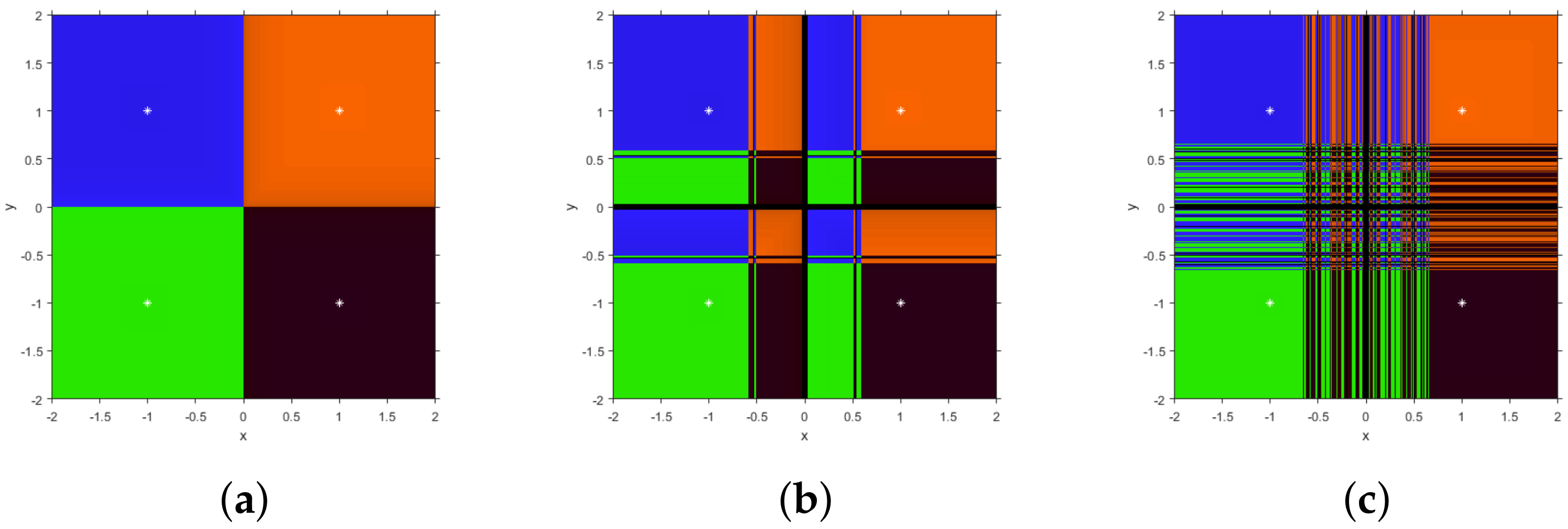
From Theorem 4, we state that convergence of SF1 on $s\left(x\right)$ is global if $a_3\in \left[-\frac{81}{8},0\right]$, as no other behavior than convergence to the roots is allowed. In Figure 1, some dynamical planes can be seen. We use a mesh M with $400\times 400$ points, and every initial guess in this mesh is iterated a maximum of 80 times with an exact error lower than ${10}^{-3}$.

Each point of M is colored depending on the root (presented as white stars) it converges to. This color is brighter when the amount of iterations needed is lower. If the maximum of iterations are reached and no convergence to the roots is achieved, then the point is colored in black. In Figure 1a, the dynamical plane of the SF1 method acting on $s\left(x\right)$ is presented. Let us notice that, for $a_3=0$, it has the same performance as Newton’s method, but with fourth-order of convergence (see Figure 1a), it is still very stable for $a_3=-5$ where the basins of attraction of the roots have infinite components (Figure 1b) and in case of $a_3=-15$ black regions of no convergence appear, but in this case they correspond to slow convergence (Figure 1c).

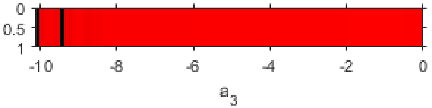
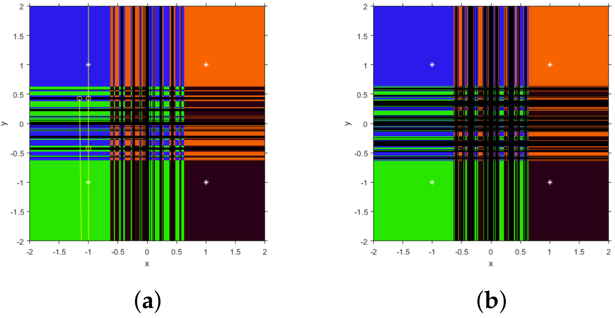
In order to find undesirable values of the parameter, we look for those members of the family that are able to converge to any other attracting element different from the roots of $s\left(x\right)$. In order to achieve this, we use the parameter line. To generate it, a free critical point depending of $a_3$ is used as initial guess for each value of $a_3$ (see Figure 2). In the interval $a_3\in \left[-\frac{81}{8},0\right]$, where there exist free critical points, each point of the mesh of 500 points is painted in red if the critical point converges to one of the roots or in black otherwise.

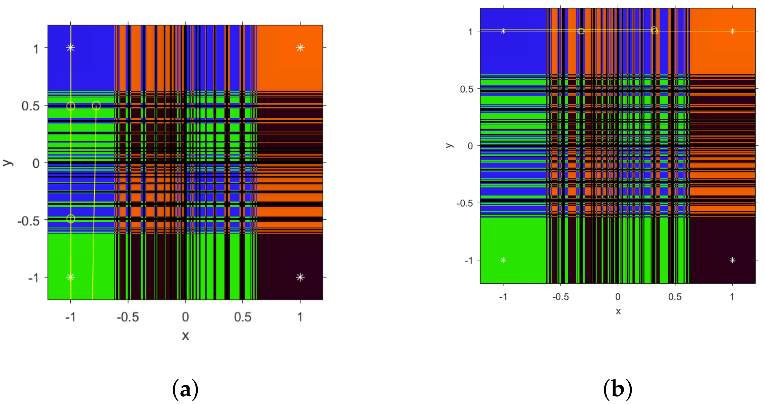
In Figure 3, different unstable cases can be found: for $a_3=-9.4$, several black areas of no convergence to the roots can be found, corresponding to four periodic orbits of period 4 (see Figure 3a)

$$\begin{array}{c}\left\{\right(-1.0000,-11.2191),(-1.0000,-0.4249),(-1.0000,11.2191),(-1.0000,0.4249\left)\right\},\\ \left\{\right(11.2191,1.0000),(0.4249,1.0000),(-11.2191,1.0000),(-0.4249,1.0000\left)\right\}\\ \left\{\right(1.0000,-11.2191),(1.0000,-0.4249),(1.0000,11.2191),(1.0000,0.4249\left)\right\},\\ \left\{\right(11.2191,-1.0000),(0.4249,-1.0000),(-11.2191,-1.0000),(-0.4249,-1.0000\left)\right\}.\end{array}$$

(15)

Similar performance can be found in Figure 3b, where the black areas correspond to periodic orbits of higher period. So, the only values of $a_3$ where convergence to attracting orbits is assured are those in black in the parameter line. In the rest of the real values, the only possible behavior is convergence to the roots of $s\left(x\right)$.

4.2. Stability of SF2

Now, let us apply the SF2 method on $s\left(x\right)=0$ and obtain its rational vectorial operator $S\left(x\right)={\left(s_1\left(x\right),s_2\left(x\right)\right)}^T$, whose j-th coordinate is

$$s_j\left(x\right)=\frac{9N_j\left(x_j\right)-2b_2{\left(x_j^2-1\right)}^6\left(81x_j^4+2x_j^2+1\right)}{9216x_j^{11}{\left(2x_j^2+1\right)}^2},j=1,2,$$

(16)

where $N_j\left(x_j\right)=909x_j^{16}+6615x_j^{14}+609x_j^{12}+1491x_j^{10}-489x_j^8+85x_j^6-5x_j^4+x_j^2$.

Therefore, we analyze the fixed points of $S\left(x\right)$ in the next result. The proof is analogous to that of SF1, so it is omitted.

Theorem 5.

Rational operator $S\left(x\right)$ related to the class of iterative methods SF2 has the roots of $s\left(x\right)$, $(1,1)$, $(1,-1)$, $(-1,1)$, $(-1,-1)$ as superattracting fixed points, but also some strange fixed points exist, whose components are the real roots of polynomial $q_1\left(t\right)=t^{14}(162b_2+28683)+t^{12}(6012-806b_2)+t^{10}(1602b_2+9747)+t^8(-1590b_2-3672)+t^6(790b_2+729)+t^4(-162b_2-36)+t^2(6b_2+9)-2b_2$ or the combination between one of these roots and $+1$ or $-1$. The number of real roots of $q_1\left(t\right)$ depends on the value of $b_2$:

• If $b_2<-\frac{3187}{18}$ or $b_2>0$, $q_1\left(t\right)$ has only two real roots and the strange fixed points are defined by combining them with themselves or with $\pm 1$.
• If $-\frac{3187}{18}\le b_2\le 0$, $q_1\left(t\right)$ has not real roots and there are not strange fixed points.

Now, it is important to study if there exist free critical points, as it is stated in the next result. Let us notice that, also in this case, there exist free critical points depending on the value of $b_2$ that can give rise to their own basins of attraction.

Theorem 6.

The rational operator $S\left(x\right)$ related to the iterative method SF2 has points $(\pm 1,\pm 1)$ as critical points. Moreover, the following cases can be described depending on the value of $b_2$:

• If $b_2\le 0$, $b_2={\displaystyle \frac{27}{8}}$ or $b_2\ge {\displaystyle \frac{101}{2}}$, then there are no free critical points.
• In other case, that is, if $0<b_2<\frac{27}{8}$ or $\frac{27}{8}<b_2<\frac{101}{2}$, the components of the free critical points are any of the two real roots of polynomial $q_2\left(t\right)=22b_2+(-81+98b_2)t^2+(-324+1238b_2)t^4+(-3645+4366b_2)t^6+(-16362+324b_2)t^8$, or any of them combined with $\pm 1$.

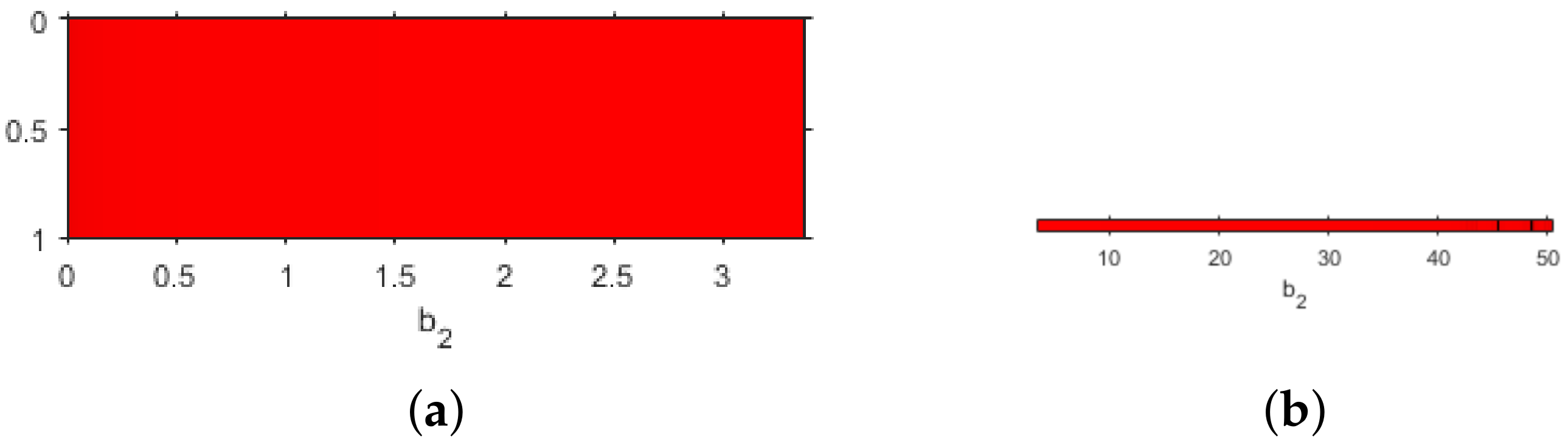
From Theorem 6, we deduce that those elements of class SF2 with values of $b_2$ satisfying $b_2\le 0$, $b_2={\displaystyle \frac{27}{8}}$ or $b_2\ge {\displaystyle \frac{101}{2}}$ can only converge to the roots of the system, achieving the most stable performance. In other cases, the parameter line help us to deduce their behavior. In Figure 4a, the line shows convergence to the roots, for both free critical points when $0<b_2<\frac{27}{8}$; however, in Figure 4b two black areas of the parameter line show the values where convergence to the roots is not guaranteed when $\frac{27}{8}<b_2<\frac{101}{2}$. In this case, the same performance also appears for any free critical point in this interval.

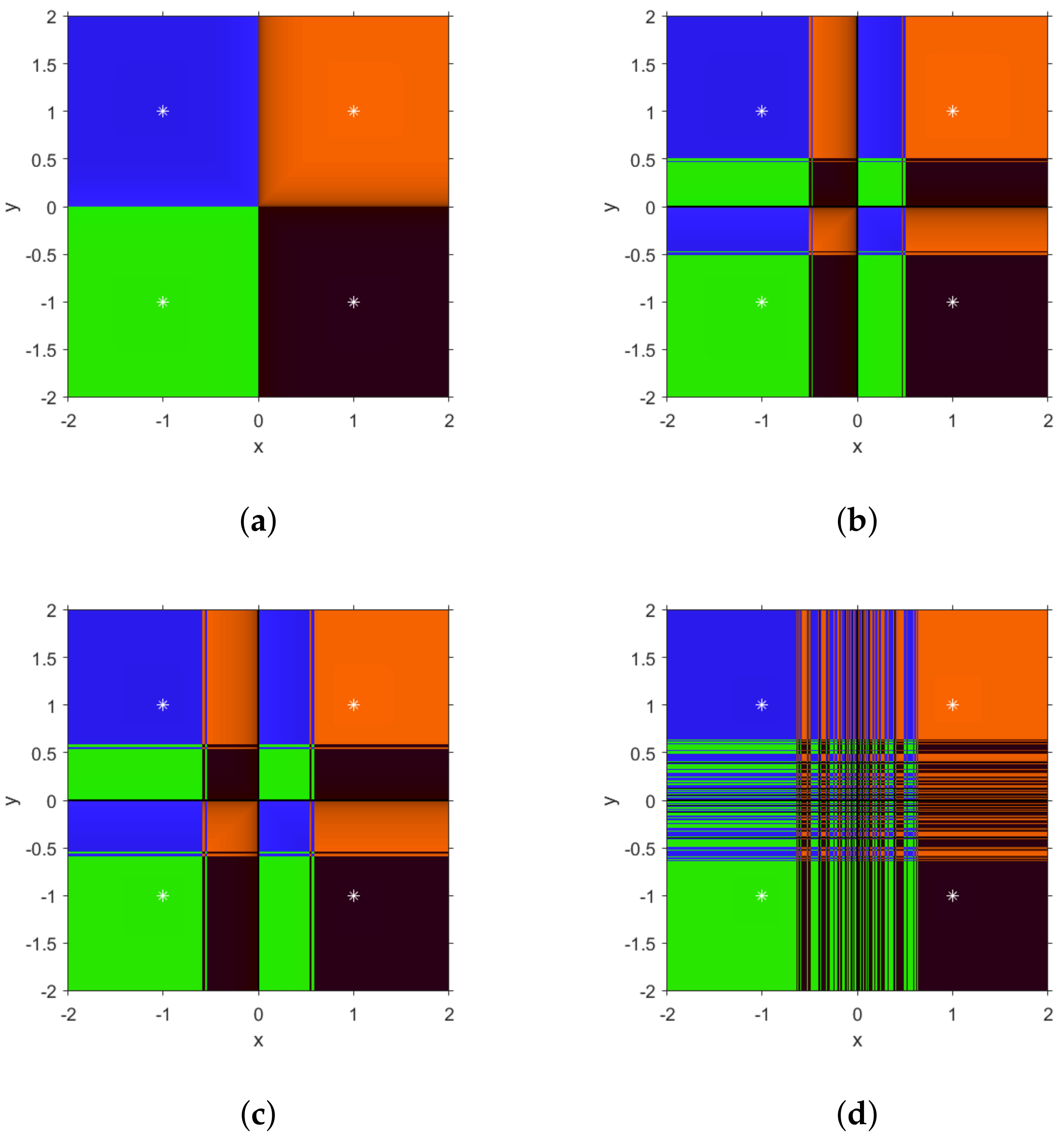
So, we can isolate values of $b_2$ in these areas of the parameter line looking for unstable behavior and choose any other value of the parameter for the stable one. In Figure 5, we observe the dynamical planes corresponding to SF2 method acting on $s\left(x\right)$ (Figure 5a). We observe that in both cases the complexity of the boundary between the basins of convergence is higher than in stable elements of SF2 and, in the case of Figure 5b, a black area of slower convergence (or even divergence) appears. The first case, for $b_2=45.5$, shows in yellow color a periodic orbit of period 4, close to one of the roots; specifically, this orbit is $\left\{\right(-1.0000,0.4919),(-1.0000,-11.7098),(-1.0000,-0.4919),(-1.0000,11.7098\left)\right\}$ and there exist other three symmetrical ones for this value of $b_2$. In Figure 5b, a similar performance with black lines corresponding to the basin of attraction of the periodic orbit

$$\left\{\right(-18.7737,1.0),(-0.3175,1.0),(2338.7,1.0),(20.5559,1.0),(0.3201,1.0),(-2136.1,1.0\left)\right\}$$

of period 6 and other symmetric ones in the vertical lines containing the roots.

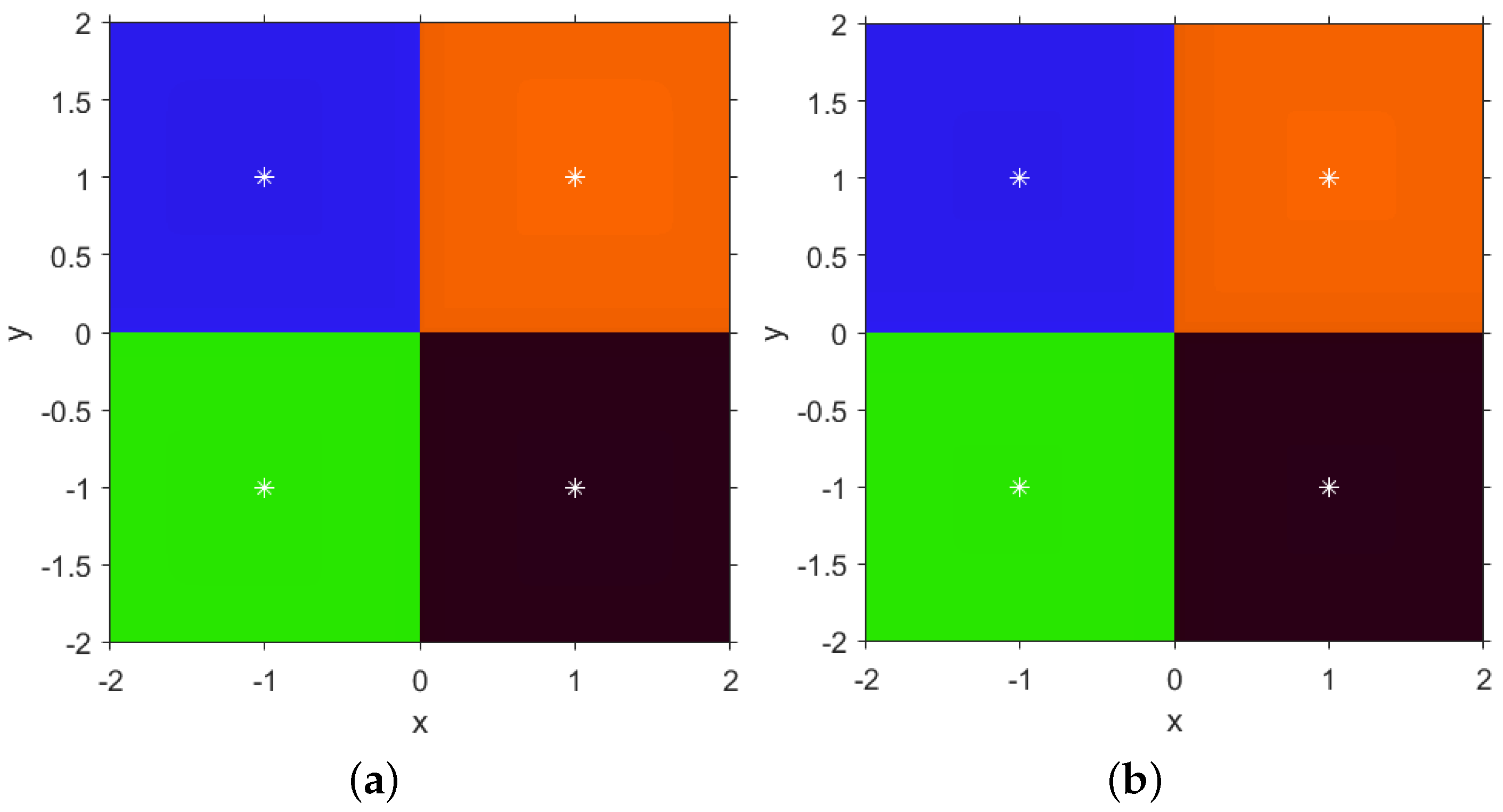
Nevertheless, the most common performance of this class of iterative methods is stability, with convergence to the roots as the only possible performance. Some examples of this behavior can be observed in Figure 6 for different values of $b_2$ with no free critical points (Figure 6a,b,d) or in the red areas of the parameter lines (Figure 6c).

4.3. Stability of SF3

Finally, let us apply the SF3 method on $s\left(x\right)=0$ and obtain its rational multidimensional operator $T\left(x\right)={\left(t_1\left(x\right),t_2\left(x\right)\right)}^T$, whose j-th coordinate is

$$t_j\left(x\right)=\frac{2\left(s_2{\left(x_j^2-1\right)}^2{m}_1\left(x_j\right)+3m_2\left(x_j\right)x_j^2\right)}{3x_j{\left(2x_j^2+1\right)}^2{\left(91x_j^4+46x_j^2+7\right)}^2\left(2s_2{\left(x_j^2-1\right)}^2+9\left({\mathrm{x}1}^4+{\mathrm{x}1}^2\right)\right)},j=1,2,$$

(17)

where $m_1\left(x_j\right)=26936x_j^{14}+166132x_j^{12}+203838x_j^{10}+115793x_j^8+38344x_j^6+7842x_j^4+938x_j^2+49$ and $m_2\left(x_j\right)=29452x_j^{16}+325588x_j^{14}+518017x_j^{12}+485983x_j^{10}+238015x_j^8+69238x_j^6+12091x_j^4+1183x_j^2+49$. Therefore, the results that give us information about the stability $T\left(x\right)$ appear below. The proofs are omitted as they are similar to the previous ones.

Theorem 7.

The rational operator $T\left(x\right)$ related to the iterative method SF3 has only the roots of $s\left(x\right)$, $(1,1)$, $(1,-1)$, $(-1,1)$ and $(-1,-1)$ as fixed points (being superattracting) if $s_2\ge 0$. However, there exist also strange fixed points, depending on negative values of $s_2$:

• If $s_2<-\frac{179409}{36218}$, the entries of the strange fixed points are the four real roots of polynomial $m_3\left(t\right)=t^{16}(144872s_2+717636)+t^{14}(1456980-77464s_2)+t^{12}(1641285-143110s_2)+t^{10}(880986-8836s_2)+t^8(44822s_2+280986)+t^6(29072s_2+54612)+t^4(9062s_2+6069)$$+t^2(1484s_2+294)+98s_2$, combined with $\pm 1$.
• If $-\frac{179409}{36218}\le s_2<0$, the entries of the strange fixed points are the two real roots of $m_3\left(t\right)$, combined with $\pm 1$.

Now, it is important to study if there exist free critical points, as it is stated in the next result. In this case there also exist points, different from the roots of $s\left(x\right)$, that make null both eigenvalues of $T{\left(x\right)}^{\prime }$.

Theorem 8.

The rational operator $T\left(x\right)$ related to the iterative method SF3 has points $(\pm 1,\pm 1)$, as the only critical points if $s_2\ge 0$. In the other case, the number of free critical points depends of the roots of polynomials of eighteenth degree.

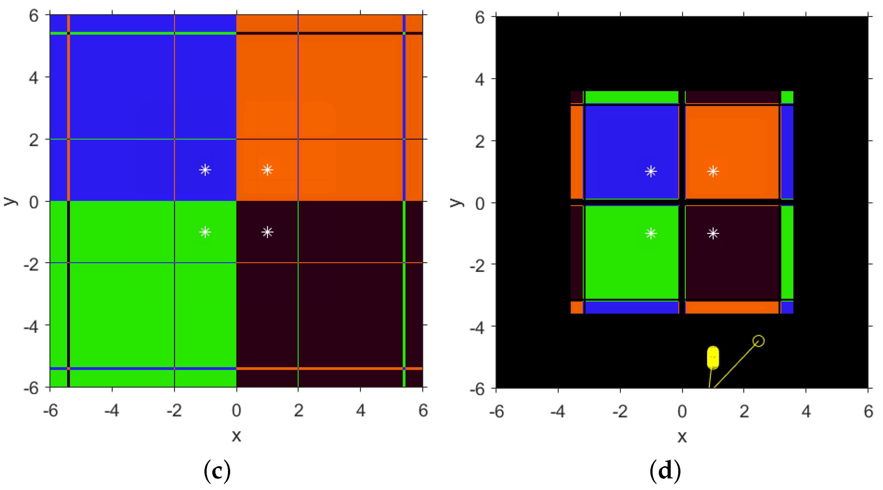
In Figure 7, the dynamical planes corresponding to SF3 method acting on $s\left(x\right)$ can be observed. Stable behavior correspond to positive or null values of $s_2$ (Figure 7a,b), meanwhile stable or unstable performance is found for some negative values of $s_2$, as can be seen in Figure 7c,d. Several attracting strange fixed points have been found for $s_2=-5.5$, whose components are $\pm 5$ and/or $\pm 1$, whose basins of attraction appear in black color.

5. Numerical Results of Fourth Order Schemes

In this section, we work on some numerical examples. We assume four mathematical problems. For the multidimensional case, the first is a kinematic synthesis problem [23,24], the second is a boundary value problem, the third is 2D Bratu’s problem and the fourth is a typical nonlinear problem [25]. We compare the behavior of SF1 with the behavior obtained by the scheme proposed by Soleymani et al. [5], denoted as FS1

$$\begin{array}{ccc}\hfill Y^{\left(n\right)}& =& X^{\left(n\right)}-\frac{2}{3}{[F^{\prime }(X^{\left(n\right)})]}^{-1}F(X^{\left(n\right)}),\hfill \\ \hfill X^{\left(n+1\right)}& =& X^{\left(n\right)}-2G({\eta }_n)H({\lambda }_n){\left[F^{\prime }(X^{\left(n\right)})+F^{\prime }(Y^{\left(n\right)})\right]}^{-1}F(X^{\left(n\right)}),\hfill \end{array}$$

where, ${\eta }_n={\left[F^{\prime }\left(X^{\left(n\right)}\right)\right]}^{-1}F\left(X^{\left(n\right)}\right)$ and ${\lambda }_n={\left[F^{\prime }\left(X^{\left(n\right)}\right)\right]}^{-1}{F}^{\prime }\left(Y^{\left(n\right)}\right),$ with

$$G\left({\eta }_n\right)=I$$

and

$$H\left({\lambda }_n\right)=I+\frac{1}{4}\left({\lambda }_n-I\right)+\frac{3}{4}{\left({\lambda }_n-I\right)}^2.$$

We have included the iteration index, $\left(n\right)$, the approximated computational order of convergence,

$$p_n=\frac{ln(inc{r}_{n+1}/inc{r}_n)}{ln(inc{r}_n/inc{r}_{n-1})},$$

the residual error of the corresponding function $∥F\left(X^{(n+1)}\right)∥$, errors between the two consecutive iterates $inc{r}_{n+1}=∥X^{(n+1)}-X^{\left(n\right)}∥$ at each step, the numerical estimation of asymptotic error estimation (AEC) and its last value, $\eta$. All computations have been done by using the software Maple 16.

Example 1.

We consider the kinematic synthesis for steering, that is described as the system of nonlinear equations

$$\begin{array}{c}{[E_j(x_{2}sin\left({\mathsf{\Psi }}_j\right)-x_3)-F_j(x_{2}sin\left({\mathsf{\Phi }}_j\right)-x_3)]}^2+{[F_j(x_{2}cos\left({\mathsf{\Phi }}_j\right)+1)-E_j(x_{2}cos\left({\mathsf{\Psi }}_j\right)-1)]}^2\hfill \\ -{[x_1(x_{2}sin\left({\mathsf{\Phi }}_j\right)-x_3)(x_{2}cos\left({\mathsf{\Phi }}_j\right)+1)-x_1(x_{2}cos\left({\mathsf{\Psi }}_j\right)-x_3)(x_{2}sin\left({\mathsf{\Phi }}_j\right)-x_3)]}^2,\hfill \end{array}$$

(18)

where $X=X^{\left(n\right)}$,

$$\begin{array}{ccc}\hfill E_j& =& -x_3{x}_2(sin\left({\mathsf{\Phi }}_j\right)-sin\left({\mathsf{\Phi }}_0\right))-x_1(x_{2}sin\left({\mathsf{\Phi }}_j\right)-x_3)+x_2(cos\left({\mathsf{\Phi }}_j\right)-cos\left({\mathsf{\Phi }}_0\right)),\hfill \end{array}$$

for $j=1,2,3$ and

$$\begin{array}{c}\hfill F_j=-x_3{x}_{2}sin\left({\mathsf{\Psi }}_j\right)+(-x_2)cos\left({\mathsf{\Psi }}_j\right)+(x_3-x_1)x_{2}sin\left({\mathsf{\Psi }}_0\right)+x_{2}cos\left({\mathsf{\Psi }}_0\right)+x_1{x}_3,\end{array}$$

$j=1,2,3$. We present the value of ${\mathsf{\Psi }}_j$ and ${\mathsf{\Phi }}_j$ in

Table 1. Value of ${\mathsf{\Psi }}_j$ and ${\mathsf{\Phi }}_j$ for (18).

i	${\mathsf{\Psi }}_{\mathit{j}}$	${\mathsf{\Phi }}_{\mathit{j}}$
0	$1.39541700417470$	$1.74617564941508$
1	$1.74448285457357$	$2.03646911277919$
2	$2.06562343694053$	$2.23909778682659$
3	$2.46006784789125$	$2.46006784098093$

. We assume the seed $X^{\left(0\right)}={(0.7,0.7.0.7)}^T$ to approximate the solution $W={(0.9051567\dots ,0.6977417\dots ,0.6508335\dots )}^T.$ The numerical results for this example are shown in

Table 2. Comparison of fourth-order methods for Example 1.

Cases	n	${\mathit{X}}^{\left(\mathit{n}\right)}$	$∥{\mathit{F}}_1\left({\mathit{X}}^{\left(\mathit{n}\right)}\right)∥$	$∥{\mathit{X}}^{(\mathit{n}+1)}-{\mathit{X}}^{\left(\mathit{n}\right)}∥$	${\mathit{p}}_{\mathit{n}}$	$\mathit{AEC}$	$\mathit{\eta }$
SF1	1	$0.920218$	$5.40036\times {10}^{-4}$	$2.20218\times {10}^{-1}$
	2	$0.905232$	$3.81192\times {10}^{-6}$	$1.49859\times {10}^{-3}$		$4.54336$	$5326.035$
	3	$0.905158$	$1.20000\times {10}^{-10}$	$1.192189\times {10}^{-4}$	$1.720052$	$5326.0353$
FS1	1	$0.914870$	$8.82812\times {10}^{-5}$	$2.148701\times {10}^{-1}$
	2	$0.905186$	$9.51730\times {10}^{-7}$	$9.68459\times {10}^{-3}$		$4.5433$	$5325.93$
	3	$0.905158$	$1.10000\times {10}^{-10}$	$4.68410\times {10}^{-3}$	$1.720058$	$5325.93$

.

Example 2.

Let we suppose a boundary value problem given by:

$$y^{″}=\frac{1}{2}{y}^3+3y^{\prime }-\frac{3}{2-x}+\frac{1}{2},\hspace{1em}\hspace{1em}y\left(0\right)=0, y\left(1\right)=1.$$

In addition, we assume the following partition of $\left[0,1\right]$:

$$x_0=0<x_1<x_2<x_3<\dots <x_n=1,$$

where $x_{i+1}=x_i+h,$ and $h=\frac{1}{m}$ such that

$$y_0=y\left(x_0\right)=0,y_1=y\left(x_1\right),\dots ,y_m=y\left(x_m\right)=1.$$

Now, we discretize the above problem with the help of first and second divided difference for approximating the derivatives.

$$y_k^{″}=\frac{y_{k+1}-y_{k-1}}{2h},y^{″}=\frac{y_{k-1}-2y_k+y_{k+1}}{h^2},k=1,2,3,\dots ,m-1.$$

In this way, we produce the $(m-1)\times (m-1)$ system of nonlinear equations

$$\begin{array}{ccc}\hfill \left(1+\frac{3h}{2}\right)y_{k-1}-2y_k+\left(1+\frac{3h}{2}\right)y_{k+1}-\frac{h^2}{2}{y}_k^3& =& \left(\frac{1}{2}-\frac{3}{2-x_k}\right)h^2,k=1,2,3,\dots ,m-1.\hfill \end{array}$$

(19)

Let us assume initial guess,

$$y_k^{\left(0\right)}={\left(\frac{1}{2},\frac{1}{2},\frac{1}{2},\frac{1}{2},\frac{1}{2},\frac{1}{2}\right)}^T.$$

In particular we solve this problem for $n=7$ so that, we obtain $6\times 6$ system of nonlinear equations. The solution of this problem is given by:

$$\begin{array}{ccc}\hfill W& =& {(0.07654393\dots ,0.1658739\dots ,0.2715210\dots ,0.3984540\dots ,0.5538864\dots ,0.7486878\dots )}^T.\hfill \end{array}$$

The numerical results are shown in

Table 3. Comparison of fourth-order methods for Example 2.

Cases	n	${\mathit{X}}^{\left(\mathit{n}\right)}$	$∥{\mathit{F}}_2\left({\mathit{X}}^{\left(\mathit{n}\right)}\right)∥$	$∥{\mathit{X}}^{(\mathit{n}+1)}-{\mathit{X}}^{\left(\mathit{n}\right)}∥$	${\mathit{p}}_{\mathit{n}}$	$\mathit{AEC}$	$\mathit{\eta }$
SF1	1	$0.748682$	$4.32119\times {10}^{-6}$	$4.23462\times {10}^{-1}$
	2	$0.748688$	$3.77602\times {10}^{-24}$	$1.06282\times {10}^{-5}$		$0.0003117$	$0.0015813$
	3	$0.748688$	$6.47000\times {10}^{-50}$	$1.40987\times {10}^{-23}$	$3.8478801$	$0.0015813$
FS1	1	$0.748682$	$4.32119\times {10}^{-6}$	$4.23462\times {10}^{-1}$
	2	$0.748688$	$3.77602\times {10}^{-24}$	$1.062820\times {10}^{-5}$		$0.0003117$	$0.0015813$
	3	$0.748688$	$3.6400\times {10}^{-50}$	$1.40987\times {10}^{-23}$	$3.8478800$	$0.0015813$

.

Example 3.

The 2D Bratu’s problem is described as:

$$u_{xx}+u_{tt}+C{e}^u=0,(x,t)\in \mathsf{\Omega },$$

(20)

with

$$\mathsf{\Omega }=[0,1]\times [0,1],$$

and boundary condition $u=0$ on $\mathsf{\Omega }$. The solution of a nonlinear partial differential equation can be estimated by means of a finite difference discretization. This reduces the problem to solving a nonlinear system. Let us assume that $w_{i,j}=u(x_i,t_j)$ is the approximated solution at grid points and that m and l are the number of steps in x and t directions, being h and k the step sizes. To solve the given PDE, we can apply the central difference to $u_{xx}$ and $u_{tt}$ respectively,

$$u_{xx}=\frac{u_{i+1,j}-2u_{i,j}+u_{i-1,j}}{h^2},\hspace{1em}{u}_{tt}=\frac{u_{i,j+1}-2u_{i,j}+u_{i,j-1}}{k^2}.$$

Then, we have the equation:

$$u_{i+1,j}+u_{i-1,j}-4u_{i,j}+u_{i,j+1}+u_{i,j-1}+h^{2}C{e}^{u_{i,j}}=0,$$

with $C=0.1$, $t\in [0,1]$ and we have the system:

$$u_{i+1,j}+u_{i-1,j}-4u_{i,j}+u_{i,j+1}+u_{i,j-1}+0.1h^2{e}^{u_{i,j}}=0.$$

(21)

We have assumed that $m=l=4$ with the initial vector of size 9,

$$\begin{array}{ccc}\hfill X^{\left(0\right)}& =& 0.1{\left(sin\left(\pi h\right)sin\left(\pi k\right),sin\left(2\pi h\right)sin\left(2\pi k\right),\dots ,sin\left(10\pi h\right)sin\left(10\pi k\right)\right)}^T.\hfill \end{array}$$

Numerical results are shown in

Table 4. Comparison of fourth-order methods for Example 3.

Cases	n	${\mathit{X}}^{\left(\mathit{n}\right)}$	$∥{\mathit{F}}_3\left({\mathit{X}}^{\left(\mathit{n}\right)}\right)∥$	$∥{\mathit{X}}^{(\mathit{n}+1)}-{\mathit{X}}^{\left(\mathit{n}\right)}∥$	${\mathit{p}}_{\mathit{n}}$	$\mathit{AEC}$	$\mathit{\eta }$
SF1	1	$0.003526$	$2.07661\times {10}^{-9}$	$9.65854\times {10}^{-2}$
	2	$0.003526$	$9.81449\times {10}^{-42}$	$8.12024\times {10}^{-10}$		$9.0723\times {10}^{-6}$	$8.2\times {10}^{-6}$
	3	$0.003526$	$5.00000\times {10}^{-52}$	$3.58063\times {10}^{-42}$	$4.005219$	$8.2329\times {10}^{-6}$
FS1	1	$0.003414$	$2.07596\times {10}^{-9}$	$9.72579\times {10}^{-2}$
	2	$0.003526$	$9.79852\times {10}^{-10}$	$8.11738\times {10}^{-10}$		$9.0722\times {10}^{-6}$	$8.4\times {10}^{-6}$
	3	$0.003526$	$7.0000\times {10}^{-52}$	$3.57364\times {10}^{-42}$	$4.005217$	$8.4233\times {10}^{-6}$

.

Example 4.

Let us assume the nonlinear Fisher’s equation with homogeneous boundary conditions of Neumann-type and the diffusion coefficient D is:

$$\begin{array}{ccc}\hfill u_t& =& D{u}_{xx}+u(1-u),\hfill \\ \hfill u(x,0)& =& 1.5+0.5cos\left(\pi x\right),0\le x\le 1,\hfill \\ \hfill u_x(0,t)& =& 0,\forall t\ge 0,\hfill \\ \hfill u_x(1,t)& =& 0,\forall t\ge 0,\hfill \end{array}$$

(22)

Now we use finite difference discretization to reduce it to a system of nonlinear equations. Let us assume that $w_{i,j}=u(x_i,t_j)$ is the approximated solution at grid points of the mesh, m and l are the number of steps in x and t directions and h and k are step sizes. Let us apply the central difference formula to $u_{xx}(x_i,t_j)$, backward difference to $u_t(x_i,t_j),$ and forward difference for $u_x(x_i,t_j),$ where $t\in [0,1]$. Then,

$$u_{i,j}^2-8D(u_{i+1,j}-2u_{i,j}+u_{i-1,j})=u_{i,j-1}.$$

In this Example, $D=1$, then the problem becomes:

$$u_{i,j}^2-8(u_{i+1,j}-2u_{i,j}+u_{i-1,j})=u_{i,j-1}.$$

(23)

For the solution of the system we have considered $m=l=4$ which reduces to a nonlinear system of size 9 with: $x_i^{\left(0\right)}=\frac{i}{{(m-1)}^2},i=1,2,\dots ,m-1.$ Numerical results are shown in

Table 5. Comparison of fourth-order methods for Example 4.

Cases	n	${\mathit{X}}^{\left(\mathit{n}\right)}$	$∥{\mathit{F}}_4\left({\mathit{X}}^{\left(\mathit{n}\right)}\right)∥$	$∥{\mathit{X}}^{(\mathit{n}+1)}-{\mathit{X}}^{\left(\mathit{n}\right)}∥$	$\mathit{COC}$	$\mathit{AEC}$	$\mathit{\eta }$
SF1	1	$88.809964$	$20066.06\times {10}^{-1}$	$887.09\times {10}^{-1}$
	2	$26.893604$	$1917.5\times {10}^{-1}$	$619.16\times {10}^{-1}$		$0.00075$	$0.00043$
	3	$61.916359$	$182.88\times {10}^{-1}$	$191.75\times {10}^{-1}$	$5.9091609$	$0.00043$
FS1	1	$10.041642$	$272.96817\times {10}^{-1}$	$99.41225\times {10}^{-1}$
	2	$2.619390$	$20.18571\times {10}^{-1}$	$74.22055\times {10}^{-1}$		$0.00075$	$0.00043$
	3	$1.696888$	$2.04109\times {10}^{-2}$	$13.19775\times {10}^{-1}$	$5.9091764$	$0.00043$

.

6. Numerical Comparison of Sixth-Order Schemes

Now, we compare the proposed schemes with those designed by Alzahrani et al. [26] denoted as (JR1),

$$\begin{array}{ccc}\hfill Y^{\left(n\right)}& =& X^{\left(n\right)}-\frac{2}{3}{[F^{\prime }(X^{\left(n\right)})]}^{-1}F(X^{\left(n\right)}),\hfill \\ \hfill T^{\left(n\right)}& =& X^{\left(n\right)}-Q({\Gamma }_n){[F^{\prime }(X^{\left(n\right)})]}^{-1}F(X^{\left(n\right)}),\hfill \\ \hfill X^{\left(n+1\right)}& =& T^{\left(n\right)}-[-2F^{\prime }{(X^{\left(n\right)})}^{-1}+6{(F^{\prime }(X^{\left(n\right)})+F^{\prime }(Y^{\left(n\right)}))}^{-1}]F(T^{\left(n\right)}),\hfill \end{array}$$

where the weight function $Q:C\to C$ is continuous given by $Q\left({\Gamma }_n\right)=12{\Gamma }_n^2-9{\Gamma }_n+\frac{5}{2}$ and differentiable function in the neighborhood of W with ${\Gamma }_n={(F^{\prime }\left(X^{\left(n\right)}\right)+F^{\prime }\left(Y^{\left(n\right)}\right))}^{-1}{F}^{\prime }\left(X^{\left(n\right)}\right)$ and $a_1,a_2\in R.$

Furthermore, we have the scheme by Behl et al. [9] denoted by (JR2),

$$\begin{array}{ccc}\hfill Y^{\left(n\right)}& =& X^{\left(n\right)}-\frac{2}{3}{[F^{\prime }(X^{\left(n\right)})]}^{-1}F(X^{\left(n\right)}),\hfill \\ \hfill T^{\left(n\right)}& =& X^{\left(n\right)}-\left(a_1+a_2{[F^{\prime }{(Y^{\left(n\right)}]}^{-1}{F}^{\prime }(X^{\left(n\right)}))}^2\right){[F^{\prime }(X^{\left(n\right)})]}^{-1}F(X^{\left(n\right)}),\hfill \\ \hfill X^{\left(n+1\right)}& =& T^{\left(n\right)}-\left({(b_2{F}^{\prime }(X^{\left(n\right)})+b_3{F}^{\prime }(Y^{\left(n\right)}))}^{-1}{F}^{\prime }(X^{\left(n\right)})+b_1{F}^{\prime }(Y^{\left(n\right)})\right)F^{\prime }{(X^{\left(n\right)})}^{-1}F(T^{\left(n\right)})\hfill \end{array}$$

where $a_1=\frac{5}{8},a_2=\frac{3}{8},b_1=2.6,b_2=-4.4$ and $b_3=8.$

All computations have been done using the software Maple 13 and we have included in

Table 6. Comparison of sixth-order methods for Example 1.

Cases	n	${\mathit{X}}^{\left(\mathit{n}\right)}$	$∥{\mathit{F}}_1\left({\mathit{X}}^{\left(\mathit{n}\right)}\right)∥$	$∥{\mathit{X}}^{(\mathit{n}+1)}-{\mathit{X}}^{\left(\mathit{n}\right)}∥$	${\mathit{p}}_{\mathit{n}}$	$\mathit{AEC}$	$\mathit{\eta }$
SF2	1	$0.908308$	$1.157258\times {10}^{-4}$	$2.08308\times {10}^{-1}$
	2	$0.905158$	$3.11000\times {10}^{-10}$	$3.21515\times {10}^{-3}$		$1.90372$	$91.1777$
	3	$0.905158$	$3.10000\times {10}^{-10}$	$2.40000\times {10}^{-9}$	$3.783584$	$91.1777$
SF3	1	$0.908833$	$5.57417\times {10}^{-5}$	$2.08832\times {10}^{-1}$
	2	$0.905158$	$4.40000\times {10}^{-10}$	$3.76250\times {10}^{-3}$		$1.97828$	$26.9455$
	3	$0.905158$	$3.20000\times {10}^{-10}$	$5.40000\times {10}^{-9}$	$3.3497758$	$26.9455$
JR1	1	$0.906593$	$3.83351\times {10}^{-4}$	$2.06592\times {10}^{-1}$
	2	$0.905158$	$8.90000\times {10}^{-10}$	$4.06564\times {10}^{-3}$		$2.23190$	$41.6145$
	3	$0.905158$	$2.20000\times {10}^{-10}$	$1.13700\times {10}^{-8}$	$3.2552278$	$41.6145$
JR2	1	$0.908646$	$5.63716\times {10}^{-5}$	$2.086463\times {10}^{-1}$
	2	$0.905158$	$1.80000\times {10}^{-10}$	$3.64084\times {10}^{-3}$		$1.92113$	$5.69106$
	3	$0.905158$	$3.20000\times {10}^{-10}$	$1.0000\times {10}^{-9}$	$3.731752734$	$5.69106$

,

Table 7. Comparison of sixth-order methods for Example 2.

Cases	n	${\mathit{X}}^{\left(\mathit{n}\right)}$	$∥{\mathit{F}}_2\left({\mathit{X}}^{\left(\mathit{n}\right)}\right)∥$	$∥{\mathit{X}}^{(\mathit{n}+1)}-{\mathit{X}}^{\left(\mathit{n}\right)}∥$	$\mathit{COC}$	$\mathit{AEC}$	$\mathit{\eta }$
SF2	1	$0.748688$	$1.12585\times {10}^{-8}$	$4.23456\times {10}^{-1}$
	2	$0.748688$	$4.00000\times {10}^{-50}$	$2.90685\times {10}^{-8}$		$0.5283261$	$0.000187$
	3	$0.748688$	$6.58000\times {10}^{-50}$	$4.0000\times {10}^{-50}$	$5.8211310$	$0.0001870$
SF3	1	$0.748688$	$1.15735\times {10}^{-8}$	$4.23456\times {10}^{-1}$
	2	$0.748688$	$6.00000\times {10}^{-50}$	$2.76367\times {10}^{-8}$		$0.0000052$	$0.000117$
	3	$0.748688$	$4.00000\times {10}^{-50}$	$7.00000\times {10}^{-50}$	$5.8117811$	$0.0001176$
JR1	1	$0.748688$	$1.00615\times {10}^{-8}$	$4.23456\times {10}^{-1}$
	2	$0.748688$	$8.00000\times {10}^{-50}$	$2.35777\times {10}^{-8}$		$0.0000041$	$0.000810$
	3	$0.748688$	$4.00000\times {10}^{-50}$	$1.20000\times {10}^{-49}$	$5.6851001$	$0.0008101$
JR2	1	$0.748606$	$4.06025\times {10}^{-3}$	$4.21306\times {10}^{-1}$
	2	$0.748688$	$3.55800\times {10}^{-7}$	$2.62289\times {10}^{-3}$		$0.0000054$	$0.000941$
	3	$0.748688$	$6.31861\times {10}^{-15}$	$3.50043\times {10}^{-7}$	$5.82719$	$0.0009412$

,

Table 8. Comparison of sixth-order methods for Example 3.

Cases	n	${\mathit{X}}^{\left(\mathit{n}\right)}$	$∥{\mathit{F}}_3\left({\mathit{X}}^{\left(\mathit{n}\right)}\right)∥$	$∥{\mathit{X}}^{(\mathit{n}+1)}-{\mathit{X}}^{\left(\mathit{n}\right)}∥$	${\mathit{p}}_{\mathit{n}}$	$\mathit{AEC}$	$\mathit{\eta }$
SF2	1	$0.003526$	$6.20\times {10}^{-15}$	$9.66\times {10}^{-2}$
	2	$0.003526$	$8.0\times {10}^{-52}$	$2.45\times {10}^{-15}$		$2.73965\times {10}^{-11}$	$2.7696$
	3	$0.003527$	$6.0\times {10}^{-52}$	$2.0\times {10}^{-52}$	$2.7495174$	$2.76962$
SF3	1	$0.003526$	$6.20\times {10}^{-15}$	$2.77\times {10}^{-2}$
	2	$0.003526$	$5.0\times {10}^{-51}$	$2.45\times {10}^{-15}$		$2.73939\times {10}^{-11}$	$8.3119$
	3	$0.003526$	$5.0\times {10}^{-52}$	$3.0\times {10}^{-52}$	$2.7144199$	$8.31199$
JR1	1	$0.003526$	$6.29\times {10}^{-15}$	$9.73\times {10}^{-2}$
	2	$0.003526$	$5.0\times {10}^{-52}$	$2.49\times {10}^{-15}$		$2.78588\times {10}^{-11}$	$7.7709$
	3	$0.003526$	$3.0\times {10}^{-52}$	$3.0\times {10}^{-52}$	$2.7164170$	$7.77098$
JR2	1	$0.003526$	$6.20\times {10}^{-15}$	$9.73\times {10}^{-2}$
	2	$0.003526$	$7.0\times {10}^{-52}$	$2.45\times {10}^{-15}$		$2.74005\times {10}^{-11}$	$2.7680$
	3	$0.003526$	$3.0\times {10}^{-52}$	$1.0\times {10}^{-42}$	$2.7495349$	$2.76800$

and

Table 9. Comparison of sixth-order methods for Example 4.

Cases	n	${\mathit{X}}^{\left(\mathit{n}\right)}$	$∥{\mathit{F}}_4\left({\mathit{X}}^{\left(\mathit{n}\right)}\right)∥$	$∥{\mathit{X}}^{(\mathit{n}+1)}-{\mathit{X}}^{\left(\mathit{n}\right)}∥$	${\mathit{p}}_{\mathit{n}}$	$\mathit{AEC}$	$\mathit{\eta }$
SF2	1	$75875.046$	$234927.08\times {10}^{-1}$	$758751.4\times {10}^{-1}$
	2	$16789.904$	$3430609.5\times {10}^{-1}$	$590861.4\times {10}^{-1}$		$6.3\times {10}^{-10}$	$4.3\times {10}^{-10}$
	3	$3716.106$	$167959.14\times {10}^{-1}$	$130737.9\times {10}^{-1}$	$5.63157$	$4.3\times {10}^{-10}$
SF3	1	$205.297$	$107037.10\times {10}^{-1}$	$2052.97\times {10}^{-1}$
	2	$34.135$	$3215.6015\times {10}^{-1}$	$1711.64\times {10}^{-1}$		$9.6\times {10}^{-8}$	$3.5\times {10}^{-8}$
	3	$3.862$	$110.1805\times {10}^{-1}$	$302.72\times {10}^{-1}$	$9.52711$	$3.5\times {10}^{-8}$
JR1	1	$44.785$	$5208.084\times {10}^{-1}$	$447.85\times {10}^{-1}$
	2	$9.297$	$258.2679\times {10}^{-1}$	$354.88\times {10}^{-1}$		$8.0\times {10}^{-5}$	$4.0\times {10}^{-5}$
	3	$1.855$	$8.724381\times {10}^{-1}$	$7.4423\times {10}^{-1}$	$6.71356$	$4.0\times {10}^{-5}$
JR2	1	$1.686$	$15.85787\times {10}^{-1}$	$15.857\times {10}^{-1}$
	2	$1.697$	$3.119860\times {10}^{-9}$	$2.2004\times {10}^{-5}$		$1.16981$	$7.3\times {10}^{-8}$
	3	$1.697$	$3.1545310\times {10}^{-33}$	$1.8000\times {10}^{-17}$	$8.26277$	$7.3\times {10}^{-8}$

the same elements as in the fourth-order schemes.

7. Conclusions

We have developed a fourth order optimal Jarratt-type family for solving nonlinear equations. High-order schemes for solving system of nonlinear equations with simple algorithmic structure are of much importance and demand. We have extended our fourth order optimal Jarratt-type family for nonlinear equations to a sixth-order family by adding only one substep and one function evaluation. We give the extension of our scheme to the system of nonlinear equations. We choose those members of the family in terms of simplicity and a vectorial stability analysis is made, showing their good properties. The ability of these schemes is checked on different test problems and it is concluded that they work better than several existing ones in the scalar case. In addition, we have also tested their working for the multidimensional case on few real life problems. The scheme SF1 works better in all cases.

References

1. Ostrowski, A.M. Solutions of Equations and System of Equations; Academic Press: New York, NY, USA, 1960. [Google Scholar]
2. Jarratt, P. Some fourth order multipoint iterative methods for solving equations. Math. Comput. 1966, 95, 434–437. [Google Scholar] [CrossRef]
3. Chun, C. Some variants of King’s fourth order family of methods for nonlinear equations. Appl. Math. Comput. 2007, 190, 57–62. [Google Scholar] [CrossRef]
4. Cordero, A.; Torregrosa, J.R.; Vassileva, M.P. Pseudocomposition: A technique to design predictor-corrector methods for systems of nonlinear equations. Appl. Math. Comput. 2012, 218, 11496–11504. [Google Scholar] [CrossRef]
5. Soleymani, F.; Khattri, S.; Vanani, S.K. The new classes of optimal Jarratt type fourth order methods. Appl. Math. Lett. 2012, 25, 847–853. [Google Scholar] [CrossRef] [Green Version]
6. Junjua, M.; Akram, S.; Yasmin, N.; Zafar, F. A new Jarratt type fourth order method for solving system of nonlinear equations and applications. Appl. Math. 2015, 2015, 805278. [Google Scholar] [CrossRef]
7. Xiao, X.Y. New techniques to develop higher order iterative methods for systems of nonlinear equations. Comput. Appl. Math. 2022, 41, 243. [Google Scholar] [CrossRef]
8. Artidiello, S.; Cordero, A.; Torregrosa, J.R.; Vassileva, M.P. Design of High-Order Iterative Methods for Nonlinear Systems by Using Weight Function Procedure. Abstr. Appl. Anal. 2015, 2015, 289029. [Google Scholar] [CrossRef] [Green Version]
9. Behl, R.; Sarria, I.; Gonzalez, R.; Magreñán, Á.A. Highly efficient family of iterative methods for solving non linear models. Comput. Appl. Math. 2019, 346, 110–132. [Google Scholar] [CrossRef]
10. Behl, R.; Arora, H. CMMSE: A novel scheme having seventh-order convergence for nonlinear systems. Comput. Appl. Math. 2022, 404, 113301. [Google Scholar] [CrossRef]
11. Hueso, J.L.; Martínez, E.; Teruel, C. Convergence, efficiency and dynamics of new fourth and sixth order families of iterative methods for nonlinear systems. Comput. Appl. Math. 2015, 275, 412–420. [Google Scholar] [CrossRef]
12. Sharma, J.R.; Arora, H. Efficient higher order derivative-free multipoint methods with and without memory for systems of nonlinear equations. Int. J. Comput. Math. 2018, 95, 920–938. [Google Scholar] [CrossRef]
13. Xiao, X.Y.; Yin, H.W. Increasing the order of convergence for iterative methods to solve nonlinear systems. Calcolo 2016, 53, 285–300. [Google Scholar] [CrossRef]
14. Wang, X. Fixed-Point Iterative Method with Eighth-Order Constructed by Undetermined Parameter Technique for Solving Nonlinear Systems. Symmetry 2021, 13, 863. [Google Scholar] [CrossRef]
15. Argyros, I.K.; Sharma, D.; Parhi, S.K.; Sunanda, S.K. On the convergence, dynamics and applications of a new class of nonlinear system solvers. Int. J. Appl. Comput. Math. 2020, 6, 142. [Google Scholar] [CrossRef]
16. Behl, R.; Bhalla, S.; Magreñán, Á.A.; Kumar, S. An efficient high order iterative scheme for large nonlinear systems with dynamics. Comput. Appl. Math. 2022, 404, 113249. [Google Scholar] [CrossRef]
17. Howk, C.L.; Hueso, J.L.; Martínez, E.; Teruel, C. A class of efficient high-order iterative methods with memory for nonlinear equations and their dynamics. Math. Meth. Appl. Sci. 2018, 41, 7263–7282. [Google Scholar] [CrossRef]
18. Zhanlav, T.; Chun, C.; Otgondorj, K. Construction and dynamics of efficient high-order methods for nonlinear systems. Int. J. Comput. Meth. 2022. [Google Scholar] [CrossRef]
19. Cordero, A.; Soleymani, F.; Torregrosa, J.R. Dynamical analysis of iterative methods for nonlinear systems or how to deal with the dimension? Appl. Math. Comput. 2014, 244, 398–412. [Google Scholar] [CrossRef]
20. Chicharro, F.I.; Cordero, A.; Garrido, N.; Torregrosa, J.R. On the effect of the multidimensional weight functions on the stability of iterative processes. Comput. Appl. Math. 2022, 405, 113052. [Google Scholar] [CrossRef]
21. Blanchard, P. Complex Analytic Dynamics on the Riemann Sphere. Bull. AMS 1984, 11, 85–141. [Google Scholar] [CrossRef] [Green Version]
22. Robinson, R.C. An Introduction to Dynamical Systems, Continuous and Discrete; Americal Mathematical Society: Providence, RI, USA, 2012. [Google Scholar]
23. Balaji, G.V.; Seader, J.D. Application of interval Newton’s method to chemical engineering problems. Reliab. Comput. 1995, 1, 215–223. [Google Scholar] [CrossRef]
24. Shacham, M. An improved memory method for the solution of a nonlinear equation. Chem. Eng. Sci. 1989, 44, 1495–1501. [Google Scholar] [CrossRef]
25. Edelstein–Keshet, L. Differential Calculus for the Life Sciences; University of British Columbia: Vancouver, BC, Canada, 2017. [Google Scholar]
26. Alzahrani, A.K.H.; Behl, R.; Alshomrani, A.S. Some higher-order iteration functions for solving non linear models. Appl. Math. Comput. 2018, 334, 80–93. [Google Scholar]
Figure 1. Dynamical planes of SF1 on s ( x ) . Blue, Orange, green and brown colors correspond to the basins of attraction of fixed points ( 1 , 1 ) , ( 1 , 1 ) , ( 1 , 1 ) and ( 1 , 1 ) , respectively. These points appears marked with white asterisks. (a) a 3 = 0 . (b) a 3 = 5 . (c) a 3 = 15 .
Symmetry 14 01742 g001
Figure 2. Parameter line of SF1 on s ( x ) for a 3 81 8 , 0 . Red and black color correspond to values of a 3 where the scheme converges to the roots or not, respectively.
Symmetry 14 01742 g002
Figure 3. Dynamical planes of unstable elements of SF1 on s ( x ) . Blue, Orange, green and brown colors correspond to the basins of attraction of fixed points ( 1 , 1 ) , ( 1 , 1 ) , ( 1 , 1 ) and ( 1 , 1 ) , respectively. These points appears marked with white asterisks. (a) a 3 = 9.4 . (b) a 3 = 10.1 .
Symmetry 14 01742 g003
Figure 4. Parameter line of SF2 on s ( x ) for (a) 0 < b 2 < 27 8 or (b) 27 8 < b 2 < 101 2 .
Symmetry 14 01742 g004
Figure 5. Dynamical planes of SF2 on s ( x ) for unstable values of b 2 . Blue, Orange, green and brown colors correspond to the basins of attraction of fixed points ( 1 , 1 ) , ( 1 , 1 ) , ( 1 , 1 ) and ( 1 , 1 ) , respectively. These points appears marked with white asterisks. (a) b 2 = 45.5 . (b) b 2 = 48.5 .
Symmetry 14 01742 g005
Figure 6. Dynamical planes of SF2 on s ( x ) for stable values of b 2 . Blue, Orange, green and brown colors correspond to the basins of attraction of fixed points ( 1 , 1 ) , ( 1 , 1 ) , ( 1 , 1 ) and ( 1 , 1 ) , respectively. These points appears marked with white asterisks. (a) b 2 = 0 . (b) b 2 = 27 8 . (c) b 2 = 20 . (d) b 2 = 60 .
Symmetry 14 01742 g006
Figure 7. Dynamical planes of SF3 on s ( x ) for stable and unstable cases. Blue, Orange, green and brown colors correspond to the basins of attraction of fixed points ( 1 , 1 ) , ( 1 , 1 ) , ( 1 , 1 ) and ( 1 , 1 ) , respectively. These points appears marked with white asterisks. Black region is the basin of attraction of attracting strange fixed points.(a) s 2 = 0 . (b) s 2 = 10 . (c) s 2 = 10 . (d) s 2 = 5.5 .
Symmetry 14 01742 g007aSymmetry 14 01742 g007b